Defining Benchmark Status: An Application using Euro-Area Bonds

This version: 17 September 2003

Peter G. Dunne, Queen's University, Belfast

Michael J. Moore, Queen's University, Belfast

Richard Portes, London Business School and CEPR

An earlier version was circulated as NBER Working Paper 9087 and CEPR Discussion

Paper 3490. The paper has benefited from seminar presentations at the London

Business School, University of Michigan, the ESRC Money Macro Finance Research

Group, the Institute for International Integration Studies, and the Irish Economic

Association. It was also presented at the NYU Salomon Center conference on ‘The

Euro: Valuation, Hedging and Capital Market Issues’. We are grateful for comments

from our discussant, Lasse Pedersen. We have also received very helpful comments

from Jim Davidson, David Goldreich, Stephen Hall, Harald Hau, Rich Lyons, Kjell

Nyborg, Carol Osler and Kathy Yuan. This paper is part of a research network on ‘The

Analysis of International Capital Markets: Understanding Europe’s Role in the Global

Economy’, funded by the European Commission under the Research Training

Network Programme (Contract No. HPRNŒCTŒ1999Œ00067). We thank Euro-

MTS Ltd for providing the data.

Defining Benchmark Status: An Application using Euro-Area Bonds

ABSTRACT

Using a unique data set from the electronic trading platform Euro-MTS, we consider

what is the ‘benchmark’ in the new euro-denominated government bond market.

Consistent with recent theoretical developments we believe that benchmark status

can be associated with characteristics of the price discovery process, and we use the

concept of Irreducibility of Cointegrating Relations among bond yields to identify the

benchmark at each maturity. We show that no one country provides the benchmark

bond at all maturities. The benchmark differs across maturities, and at some

maturities benchmark status is shared by the bonds of more than one country.

Keywords: benchmark, euro government bonds, cointegration JEL: F36, G12, H63 Peter G. Dunne (Queen's University, Belfast) The Queen's University of Belfast School of Management & Economics Belfast BT 7 1NN Northern Ireland e-mail: p.dunne@qub.ac.uk Telephone: +44 (028) 90273310 Fax: +44(028) 90328649 Michael J. Moore (Queen's University, Belfast) The Queen's University of Belfast School of Management & Economics Belfast BT 7 1NN Northern Ireland e-mail: m.moore@qub.ac.uk Telephone: +44 (028) 90273208 Fax: +44(028) 90328649 Richard Portes (London Business School and CEPR)

Department of Economics London Business School Sussex Place Regent’s Park London NW1 4SA Tel. (+44 20) 7706 6886 Fax ((+44 20) 7724 1598 Email rportes@london.edu

Corresponding author: Richard Portes, Columbia Business School, 822 Uris Hall, 3022 Broadway, New York NY 10027-6902, tel. 212-854-1753, email rp2128@columbia.edu

1

Defining Benchmark Status: An Application using Euro-Area Bonds

Peter G. Dunne (QUB)

Michael J. Moore (QUB)

Richard Portes (LBS, NBER and CEPR)

1. Introduction

The introduction of the euro on 1 January 1999 eliminated exchange risk

between the currencies of participating member states and thereby created the

conditions for a substantially more integrated public debt market in the euro area.

The euro-area member states agreed that from the outset, all new issuance should

be in euro and outstanding stocks of debt should be re-denominated into euro. As a

result, the euro-area debt market is comparable to the US treasuries market both in

terms of size and issuance volume. Unlike in the United States, however, public debt

management in the euro area is decentralised under the responsibility of 12 separate

national agencies.

This decentralised management of the euro-area public debt market is one

reason for cross-country yield spreads. But the evidence of differentiation across

countries has not been thoroughly explored, and one of the contributions of this

paper is to describe patterns in cross-country yield differences. For example, we find

yields are lowest for German bonds; that there is an inner periphery of countries

centred on France for which yields are consistently higher; and that the outer

periphery centred on Italy displays the highest yields.

2

We begin our analysis by discussing why such yield spreads exist. Our main

contribution, however, comes in examining benchmark status. In this decentralised

euro government bond market, there is no official designation of benchmark

securities, nor any established market convention. Indeed, benchmark status is more

or less explicitly contested among countries.

One might ask why this should be so, aside from national pride. What are the

benefits of achieving benchmark status? This leads us to consider the appropriate

definition of ‘benchmark’. If the ‘benchmark’ were simply the security with lowest

yield, the question would answer itself: clearly governments wish to borrow at the

lowest possible yields; and there is an obvious welfare consequence, if foreigners

hold any significant share of domestic government securities.

If indeed lowest yield were all that mattered for benchmark status, then the

German market would provide the benchmark at all maturities (see below). Analysts

who take this view accept that the appropriate underlying criterion for benchmark

status is that this is the security against which others are priced, and they simply

assume that the security with lowest yield takes that role (e.g., Favero et al., 2000,

pp. 25-26). A plausible alternative, however, is to interpret benchmark to mean the

most liquid security1, which is therefore most capable of providing a reference point

for the market. But the Italian market, not the German, is easily the largest and

arguably the most liquid for short-dated bonds; and perhaps the French is most liquid

at medium maturities.

3

Liquidity is to some extent quantifiable, but liquidity alone is unlikely to be a

reliable identifier of benchmark status. For example, Italian bonds are most liquid at

almost all maturities but the Italian long yield is probably too variable to be a good

reference point, or a suitable hedge, for other parts of the market. The characteristic

of being a reference point for the market is something that closely relates to Yuan’s

(2002) definition of a benchmark, as discussed below. We also believe it is possible

to distinguish the benchmark empirically, given that the benchmark is defined this

way. So our approach focuses directly on the price discovery process to reveal

benchmark status (see Hasbrouck, 1995, for a treatment in the context of equity

markets). Indeed, one of the attractions of benchmark status is that benchmark

bonds are held by a wide international base of investors, who often provide an

unofficial market in the benchmark outside normal trading hours. This in turn makes

them more representative of the market.

Yuan’s model employs an exogenously determined benchmark. We expect that

similar attributes would be possessed by an endogenously determined benchmark,

however, and we modify Yuan’s model to fit the Euro-area bond market in this and

other respects. Endogeneity in the emergence of the benchmark is not of central

importance to our identification methodology. If the benchmark bond has benchmark

traits consistent with those outlined by Yuan, then our methodology should be

capable of identifying it as the benchmark.

4

The model of Yuan closely associates benchmark status with the price

discovery process. Once in existence the benchmark security provides an

information externality to the market as a whole because it best represents common

movements of the entire market. Essentially, the benchmark bond is the instrument

to which the prices of other bonds react. On this view, the identification of

benchmark status must emerge from empirical analysis and cannot simply be

asserted or read off the data. A benchmark security concentrates the aggregation of

information and reduces the cost of information acquisition in all markets where a

security is traded against the benchmark.

Since price discovery is central to our definition of benchmark status, we

consider alternative approaches to identifying the price discovery process. Scalia

and Vacca (1999) for example, use Granger-Causality tests to determine whether

price discovery occurs in the cash or futures market in Italian bonds. In the context

of identifying benchmark status, however, we believe that Granger-Causality testing

exhibits significant weaknesses, particularly in the context of high-frequency

transaction data with variable liquidity. We nevertheless begin our empirical analysis

by conducting tests for Granger causality between yields. If a bond yield at a

particular maturity Granger-causes the yields of bonds in other countries at the same

maturity, this suggests that the Granger-causing bond is the benchmark at that

maturity. Despite the simple appeal of this technique and our strenuous efforts to

avoid the worst effects of its weaknesses, we prefer to regard this part of our analysis

as descriptive, and we place more weight on the novel approach we introduce in

section 5.2.

This alternative empirical method exploits the fact that yields are non-stationary

for every country and at every maturity. If there were a unique benchmark at every

maturity, then we would expect that the yields of other bonds would be cointegrated

with that benchmark. Indeed, there should be multiple cointegrating vectors

centering on the benchmark bond. This empirical approach relies on a result, based

on Davidson (1998), that the structural nature of the cointegrating relationship

between a benchmark bond and other bonds can be identified even in the context of

quite a general theoretical framework. We outline this approach in detail in section 5.

5

In the next section, we discuss the structure and development of the market for

euro-area government bonds. Section 3 provides an explicit theoretical framework

within which a benchmark security is defined and we consider the implications of this

framework for the identification of the benchmarks in the euro-denominated

government bond market. Section 4 describes our unique data set. Section 5

presents the novel empirical methodology and analysis and section 6 concludes.

6

2. The market for euro-area government bonds

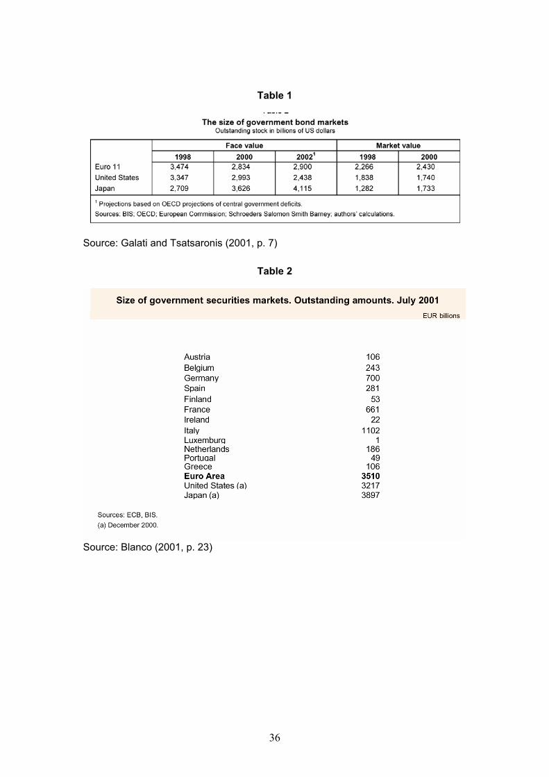
The euro-area government bond market, at just under USD 3 trillion, is

somewhat larger than that of the United States (Table 1). The largest outstanding

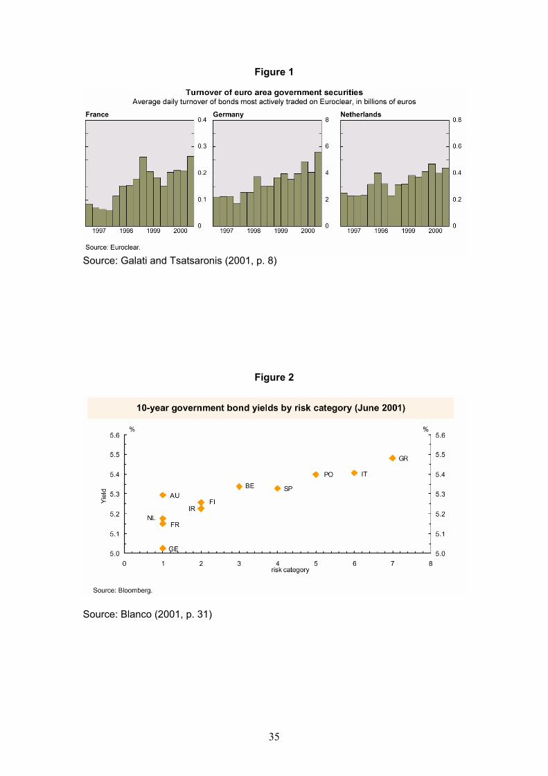
stocks are those of Italy, Germany and France, in that order (Table 2). Turnover has

risen dramatically since 1998 – by a factor of three for France, for example (Figure

1). International participation has also risen rapidly: in the three years from 1997 to

2000, the share of Belgian bonds held by non-residents rose from 29% to 53%

(Galati and Tsatsaronis, 2001); for France, it doubled to reach one-third, which was

also the average for the entire area (ibid. and Blanco, 2001).

McCauley (1999) draws some comparisons between the US municipal bond

market and the euro government bond markets, but there can be no question that the

latter are much more highly integrated. There has been considerable convergence

among countries in the structure and maturities of government debt. The share of

foreign-currency debt has fallen to negligible levels, mainly because that formerly

denominated in other euro-area currencies is now denominated in euros. Each

country is striving to achieve large liquid benchmark-size issues: recent French and

Italian issues have exceeded € 20 bn, putting them at the level of US Treasury

benchmark issues. German issues are in the range of € 10-15 bn, and even the small

countries are now up to € 3-5 bn issue size. Secondary markets have become much

deeper and more efficient (see Favero, et al., 2000).

7

There are still significant impediments to market integration. The single

currency has not brought unification of tax structures, accounting rules, settlement

systems, market conventions, or issuing procedures. On the other hand, a single

electronic trading platform now handles about half of the total volume of secondary

market transactions (see below).

Nor has market integration gone so far as to give identical yields on different

countries’ securities of the same characteristics. Yields have indeed converged. But

there are still significant spreads, and since mid-2000, though not before, all

countries have had positive spreads relative to Germany at all maturities (until very

recently). In our data (see below), for example, the Italian-German yield gap ranges

from 18 bp at the short end to 35 bp at the very long end2. Some observers conclude

that this gives Germany unambiguous status as the benchmark issuer, although

there might have been some multiplicity in the first eighteen months of EMU (Blanco,

2001, p. 14-15, Codogno, et al., 2003).

8

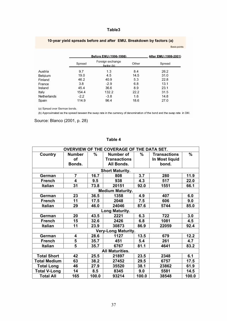
What are the sources of these yield differentials? It is plausible that before

EMU, much of the spread simply reflected exchange-rate risk. Indeed, by comparing

swap rates, Blanco (2001, Sec. 4.1) breaks down the spreads over German yields at

the 10-year maturity between the foreign exchange factor and other factors, which he

identifies with credit (default) risk and microstructure characteristics, in particular

liquidity. He finds that for those countries with wide pre-1999 spreads, the main

component was exchange-rate risk (Table 3). Moreover, taking that factor out,

spreads have in fact widened significantly for all countries since the advent of the

euro. And insofar as bond ratings represent default risk, it seems clear that only part

of these wider spreads is attributable to this factor (in Figure 2, we see substantial

differences in yields between countries in the same risk category). But the

interpretation of the spreads as representing different credit risks and liquidity

characteristics is also problematic, and establishing which of these factors is

dominant is even more difficult (Portes, 2003). The spreads vary over time and along

the yield curve. But credit ratings vary very little indeed over time and typically do not

discriminate across maturities; and we are far from being able to identify time-varying

and maturity-dependent determinants of liquidity.

Whatever the causes of the spreads for other countries over German yields,

the mere fact that they are positive is enough for most observers to conclude that

Germany provides the benchmark all along the yield curve. We shall find that the

dynamic evidence on price discovery suggests a very different view.

9

3. Benchmark securities: a framework

Yuan (2002) formalises the concept of a benchmark security. Adopting her

definition to our context, define a country-specific security as having a yield with the

following factor structure:

(1) % 1.....,fi i i ir r i nβ γ ε= + + =

where is the return on the ith country’s security, irfir is the country-specific risk-free

rate. The risk-free rate can differ across countries because of, for example, political

factors such as the possibility that a country might leave the euro-zone. %γ is euro-

zone wide risk and iβ is country i’s sensitivity to that risk. iε is the country-specific

shock.

As usual, i ∀ = are stationary processes that are independently

distributed normally with mean zero and variance

1.....,iε n

2iσ . But we depart from

convention, including Yuan’s specification, with regard to the systematic risk %γ . We

assume that %γ is an I(1) process3. Consequently, all of the yields are themselves

non-stationary.

At this point, it is worth showing the following result:

Lemma 1. All pairs of country yields { }, 1....,ir i n= are cointegrated.

Proof: For any equation (1) implies that and ir jr

ff

j ji i i

i j i j i j

r rr r jεεβ β β β β β

− = − + −

10

The right hand side is stationary by assumption. The cointegrating vector is 1 1,i jβ β

−

.

Note that the variance of the cointegrating residual is:

22

2Var ji i

i j i

rr2j

j

σσβ β β β

− = +

(2)

We are now in a position to define a benchmark security:

Definition 1 (Yuan): A benchmark security has the following two properties:

(i) it has no sensitivity to country-specific risk,

(ii) it has unit sensitivity to systematic risk.

In our case, systematic risk is the euro-zone risk %γ . The benchmark security can be

constructed as follows. Form the following basket of country-specific securities:

%1 1 1

1 1with 0 and 1

n n nf

b i i i i i ii i i

n n

i i i ii i

r w r w w

w w

β γ ε

ε β

= = =

= =

= + +

→ →

∑ ∑ ∑

∑ ∑where are the weights on each country’s security. In effect, the

benchmark security’s yield, r , is:

1.....,iw i n=

b

(3)

%

1

where

fb b

nfb i

i

r r

r w

γ

=

= +

=∑ fir

It is noteworthy that within this framework there is no explicit role for the level of the

yield. While benchmark status may give rise to lower yields, here it is assumed that

benchmark attributes stem purely from characteristics related to the security’s

information content.

11

Lemma 2. All country yields { }, 1....,ir i n= are pairwise cointegrated with the

benchmark yield r . b

Proof:

From equations (1) and (3),

f

fi ib b

i i

r rr r i

i

εβ β β

− = − +

The right hand side is stationary by assumption. The cointegrating vector is

1 , 1iβ

−

.

Note that the variance of the cointegrating residual is:

2

2Var ib

i i

r r iσβ β

− =

(4)

We are now in a position to state the main result:

Theorem 1:

The variance of the residual error in the cointegrating vector between the yield on

country i’s security and any other country specific security j=1…,n. is always greater

than the variance of the residual error in the cointegrating vector between country j’s

yield and the benchmark yield.

Proof: Compare equations (2) and (4).

The above results have been developed using the property that the

benchmark is a basket of bonds. The concept of a benchmark security as a basket

of bonds is not entirely new. Galati and Tsatsaronis (2001) raise the idea in the

context of euro-area government bonds, only to dismiss it immediately: ‘Market

12

participants, however, are not yet ready to accept a benchmark yield curve made up

of more than one issuer, being wary of the problems posed by small but persistent

technical differences between the issues that complicate hedging and arbitrage

across the maturity spectrum (p. 10).’

The analysis above is predicated on the idea that the benchmark bond is

issued exogenously. In the euro-area bond market, however, this cannot occur. We

argue, instead, that a particular country’s bond emerges endogenously as the

benchmark, at each maturity, with the characteristics outlined in Definition 1.

Whether or not the benchmark is endogenously determined, Yuan’s analysis

regarding its characteristics is likely to hold true. The contest for benchmark status

may itself be worth modelling, but here we restrict attention to the more modest task

of identifying the benchmarks at each maturity. We believe that the empirical

approach we use is capable of identifying the benchmark independent of the nature

of the contest for benchmark status.

In section 5.2, we introduce the methodology for implementing Theorem 1. The

methodology was originally proposed by Davidson (1998) and modified by Barassi,

Caporale and Hall (2000 a, b). Davidson’s original work has direct parallels with the

statistical result used by Yuan to motivate her concept of a benchmark. We return to

the idea of the benchmark as a basket of bonds in section 5.3.

13

4. Data

4.1 Primary data

We have a unique transactions-based data set from Euro-MTS for October and

November of 2000. Since the creation of the euro in 1999, Euro-MTS has emerged

as the principal electronic trading platform for bonds denominated in euros. At the

end of 2000, it handled over 40% of total transactions volume (Galati and

Tsatsaronis, 2001). Government bonds traded on Euro-MTS must have an issue size

of at least € 5 bn. For a discussion of MTS, see Scalia and Vacca (1999).

The full data set consists of all actual transactions. For each transaction, we

have a time stamp, the volume traded, the price at which the trade was conducted

and an indicator showing whether the trade is initiated by the buyer or seller. The

countries represented are Germany, Finland, Portugal, Spain, Austria, Italy, France,

the Netherlands and Belgium: all euro-area countries except Ireland4. Greece joined

the euro-area after the time-period covered by the sample, while the twelfth euro-

area country, Luxembourg, has negligible government debt.

The sample includes all Euro-MTS and country-specific MTS bonds traded on

the electronic platforms. In addition to treasury paper, the data set also includes

French and German mortgage-backed bonds, a European Investment Bank bond,

and a euro-denominated US agency bond (“Freddie-Mac”).

4.2 Derived data

In the analysis below we use the most frequently traded bond on the EuroMTS

platform for each of three countries (Italy, France and Germany) and for each of four

14

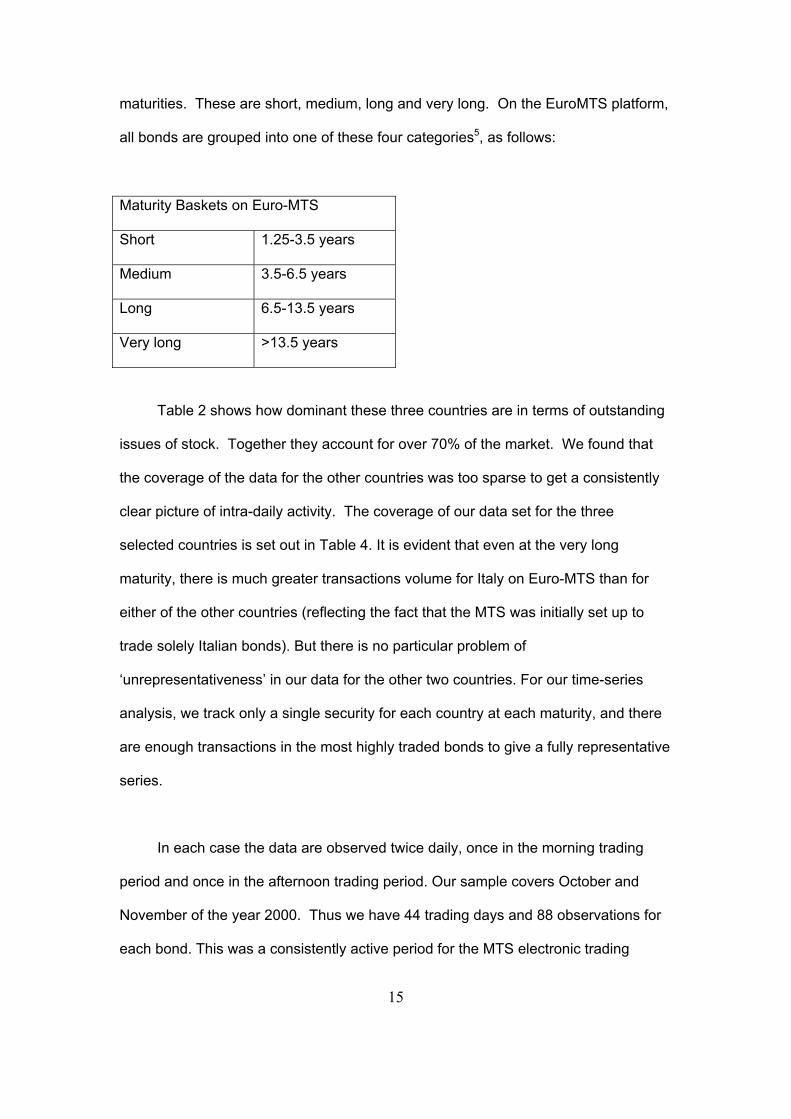
maturities. These are short, medium, long and very long. On the EuroMTS platform,

all bonds are grouped into one of these four categories5, as follows:

Maturity Baskets on Euro-MTS

Short 1.25-3.5 years

Medium 3.5-6.5 years

Long 6.5-13.5 years

Very long >13.5 years

Table 2 shows how dominant these three countries are in terms of outstanding

issues of stock. Together they account for over 70% of the market. We found that

the coverage of the data for the other countries was too sparse to get a consistently

clear picture of intra-daily activity. The coverage of our data set for the three

selected countries is set out in Table 4. It is evident that even at the very long

maturity, there is much greater transactions volume for Italy on Euro-MTS than for

either of the other countries (reflecting the fact that the MTS was initially set up to

trade solely Italian bonds). But there is no particular problem of

‘unrepresentativeness’ in our data for the other two countries. For our time-series

analysis, we track only a single security for each country at each maturity, and there

are enough transactions in the most highly traded bonds to give a fully representative

series.

In each case the data are observed twice daily, once in the morning trading

period and once in the afternoon trading period. Our sample covers October and

November of the year 2000. Thus we have 44 trading days and 88 observations for

each bond. This was a consistently active period for the MTS electronic trading

15

platform, and it was a period within which there was increased uncertainty regarding

benchmark status due to the relatively recent nature of the conversion to euro

denomination. More recently the decline of the non-German bond futures markets

may suggest that Germany is once again in the dominant benchmark position, but we

find that German dominance was not at all clear in the period we study. Thus, our

analysis provides some indication of how susceptible German dominance might be to

future threats such as the possibility of a downgrading of German bonds if German

fiscal and macroeconomic conditions were to deteriorate significantly.

The availability and timing of observations is important, especially for causality

testing6. In our case, the transactions for each variable were chosen according to

their closeness in time to (either before or after) the last available transaction in each

period in the least-liquid bond7. Hence, the observations are not necessarily close to

the end of the trading period. This minimises the time gap between observations.

16

Interpolation was done in relatively few cases (never for the Italian) and almost

always involved the use of the most similar bonds from the same country (i.e. similar

in terms of maturity, coupon, liquidity, and the yield gap against the other two

countries). In the case of the long bonds, interpolation of the French benchmark was

sometimes done using the most similar Dutch bond. In the instances where

interpolation was not possible, the previously observed yield was continued forward.

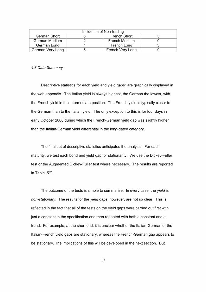
The table below shows how often this was necessary. It is worth pointing out that the

periods of greatest illiquidity were also the periods of least variability, so that our

practice of assuming zero change is not likely to have had large effects on our

results, with one exception. Despite our efforts to avoid the problems arising from

non-trading, the conclusions of our Granger-causality testing are consistent with

bonds of higher liquidity appearing to cause the less liquid bond yields8.

Incidence of Non-trading

German Short 6 French Short 3 German Medium 2 French Medium 0

German Long 1 French Long 3 German Very Long 5 French Very Long 9

4.3 Data Summary

Descriptive statistics for each yield and yield gaps9 are graphically displayed in

the web appendix. The Italian yield is always highest, the German the lowest, with

the French yield in the intermediate position. The French yield is typically closer to

the German than to the Italian yield. The only exception to this is for four days in

early October 2000 during which the French-German yield gap was slightly higher

than the Italian-German yield differential in the long-dated category.

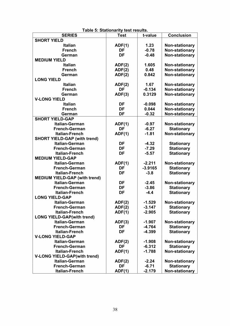
The final set of descriptive statistics anticipates the analysis. For each

maturity, we test each bond and yield gap for stationarity. We use the Dickey-Fuller

test or the Augmented Dickey-Fuller test where necessary. The results are reported

in Table 510.

The outcome of the tests is simple to summarise. In every case, the yield is

non-stationary. The results for the yield gaps, however, are not so clear. This is

reflected in the fact that all of the tests on the yield gaps were carried out first with

just a constant in the specification and then repeated with both a constant and a

trend. For example, at the short end, it is unclear whether the Italian-German or the

Italian-French yield gaps are stationary, whereas the French-German gap appears to

be stationary. The implications of this will be developed in the next section. But

17

Lemma 1 in Section 2 shows that we should not necessarily expect yield gaps to be

stationary.

18

5. Results and analysis

5.1 Granger causality

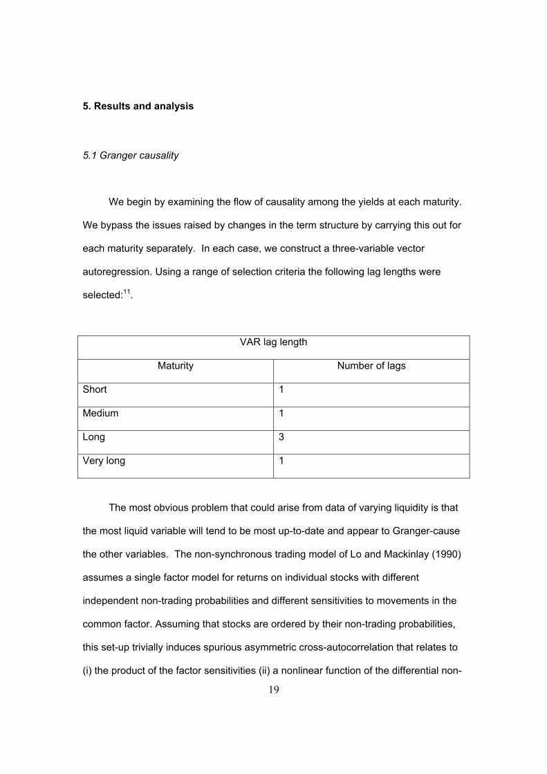
We begin by examining the flow of causality among the yields at each maturity.

We bypass the issues raised by changes in the term structure by carrying this out for

each maturity separately. In each case, we construct a three-variable vector

autoregression. Using a range of selection criteria the following lag lengths were

selected:11.

VAR lag length

Maturity Number of lags

Short 1

Medium 1

Long 3

Very long 1

The most obvious problem that could arise from data of varying liquidity is that

the most liquid variable will tend to be most up-to-date and appear to Granger-cause

the other variables. The non-synchronous trading model of Lo and Mackinlay (1990)

assumes a single factor model for returns on individual stocks with different

independent non-trading probabilities and different sensitivities to movements in the

common factor. Assuming that stocks are ordered by their non-trading probabilities,

this set-up trivially induces spurious asymmetric cross-autocorrelation that relates to

(i) the product of the factor sensitivities (ii) a nonlinear function of the differential non-

19

trading probabilities and (iii) the ratio of the variance of the common factor to the

product of the individual security standard deviations. In our data we would expect

the factor sensitivities to be near 1. We would expect the ratio of the variance of the

common factor to the product of individual standard deviations to be also near unity.

Under these circumstances, where π is the non-trading probability, the calculation of

the spurious nth order cross-autocorrelation between the ith and jth bond returns can

be performed using;

(1 )(1 )

1i jn n

ij ii j

π πρ π

π π− −

≈−

In our case, we can see that any cross-autocorrelation with the Italian return as the

reference variable would be zero due to a zero Italian non-trading probability

( 0iπ = ). However, the French and German yields should appear to be Granger-

caused by the Italian because these usually have positive non-trading probabilities.

Since the German bonds have the highest non-trading probabilities the Granger-

causality testing should be biased against the German as the benchmark.

The Granger Causality Test results on the whole appear to confirm these

priors12. At the short end no country emerges as benchmark. Non-causality is

rejected in every case: lagged yields of each country affect the yields of one or both

of the other countries. For the medium maturity, where neither the Italian nor the

French bond suffer from the stale price problem, the German bond can be ruled out

as a possible benchmark, but both the Italian and French yields have predictive

power for other countries’ yields. At the long end the Italian bond emerges as a

benchmark and has predictive power for both French and German yields. Finally, for

the very long maturity, as with the medium maturity, only the German bond can be

ruled out as benchmark.

20

These results strongly reject the hypothesis that innovations in German yields

Granger-cause innovations in French and Italian yields, at all maturities. That

interpretation of Germany as the benchmark issuer is not consistent with our data.

We would not wish to place too high a weight on these results, however, partly

because of the weaknesses of the approach in the presence of missing observations,

and more particularly because the analysis of section 2 gives no role for causality in

the definition of a benchmark.

5.2 Cointegration

The Granger-causality analysis is simple but perhaps rather crude. It ignores

long-run relationships. The factor definition of a benchmark in section 3 along with

Lemmas 1 and 2 as well as Theorem 1 suggests that the benchmark should be

identified from an analysis of the cointegration properties of the yield series. Despite

the use of a basket of bonds as benchmark in the analysis of section 3, in this section

we entertain the idea that a single country’s bonds could possess benchmark

characteristics. If a particular country provides the benchmark at a given maturity,

then there should be two cointegrating vectors in the three-variable system of country

yields. For example, if Germany were the benchmark, then the cointegrating vectors

could be13

Italian yield = γGerman yield + nuisance parameters

French yield = δGerman yield + nuisance parameters

.

21

But this approach suffers from an identification problem. Even if we are

satisfied that cointegration vectors along the lines of the above exist, we still cannot

draw any immediate conclusion about the structure of the relationships between

yields such as the identity of the benchmark. The reason for this is that any linear

combination of multiple cointegrating vectors is itself a cointegrating vector. In

particular,

Italian yield = (γ/δ)French yield + nuisance parameters

provides us with a perfectly valid cointegrating vector derived from the above. On the

face of it, any one of the yields can provide the benchmark, and we have made no

progress.

A recent development in non-stationary econometrics due to Davidson (1998)

and developed by Barassi, Caporale and Hall (2000 a,b) [BCH] enables us to

explore the matter further. This involves testing for irreducibility of cointegrating

relations and ranking according to the criterion of minimum variance. The interesting

feature of this method is that it allows us to learn about the structural relationship that

links cointegrated series from the data alone, without imposing any arbitrary

identifying conditions. In this case, the ‘structural’ relationship that we are exploring is

the identity of the benchmark in a set of bond yields.

There is a risk of confusion in the use of the word ‘structure’, because of the

many different uses to which it has been put by different authors. Davidson uses the

term to mean parameters or relations that have a direct economic interpretation and

may therefore satisfy restrictions based on economic theory. It need not mean a

22

relationship that is regime-invariant. The possibility that “incredible assumptions”

(Sims, 1980) need not always be the price of obtaining structural estimates turns out

to be a distinctive feature of models with stochastic trends.

We begin with the concept of an irreducible cointegrating vector.

Definition 2 (Davidson): A set of I(1) variables is called irreducibly cointegrated (IC)

if they are cointegrated, but dropping any of the variables leaves a set that is not

cointegrated.

IC vectors can be divided into two classes: structural and solved. A structural IC

vector is one that has a direct economic interpretation.

Theorem 2 (Davidson). If an IC relation contains a variable which appears in no

other IC relation, it is structural.

The less interesting solved vectors are defined as follows:

Definition 3 (Davidson). A solved vector is a linear combination of structural

vectors from which one or more common variables are eliminated by choice of

offsetting weights such that the included variables are not a superset of any of the

component relations.

A solved vector is an IC vector which is a linear combination of structural IC

vectors. Once an IC relation is found, interest focuses on the problem of

distinguishing between structural and solved forms. Of course, the theoretical model

might answer this question for us, but this would then simply be using the theory to

23

identify the model, so in the absence of overidentifying restrictions we could learn

nothing about the validity of the theory itself. The key issue is whether we can

identify the structure from the data directly.

BCH introduce an extension of Davidson's framework that can be illustrated

concretely with our problem as follows. In our system made up of three I(1)

variables, the French, German and Italian bond yields, consider the case where the

pairs (German yields, French yields) and (German yields, Italian yields) are both

cointegrated. It follows necessarily that the pair (French yields, Italian yields) is also

cointegrated. The cointegrating rank of these three variables is 2, and one of these

three IC relations necessarily is solved from the other two. The problem is that we

cannot know which, without a prior theory. Here is where the BCH extension of

Davidson's methodology shows its effectiveness. In order to detect which of the

cointegrating relations is the solved one and which of the vectors are irreducible and

structural, we calculate the descriptive statistics of each cointegrating relation and

rank these vectors on the basis of the magnitude of the variance of their residual

errors. The structural vectors are identified as the ones corresponding to the lowest

variance. The reason for this is suggested by standard statistical theory and can be

illustrated as follows: Let x, y and z be our cointegrated series and let

y - βx = e1

y - γz = e2

x - δz = e3

be the three irreducible cointegrating relations. Now assume that the structural

relationships are the first two, (y-βx and y-γz), with e1 and e2 being the structural

24

error terms from the first two which are therefore assumed14 to be distributed

independently N(0, 2iσ ), i=1,2. The third equation is just solved from the first two15.

This implies that e3 is a function of e1 and e2, and therefore we expect it to be

distributed N(0,2 21

22σ σ

β+

). If { }2 23 11 then ,Max 2

2β σ σ≤ > σ . The

condition 1 β ≤ holds in every case that we estimate below. Since there exists an

alternative linear combination of the structural relations that could result in the solved

relation with γ as the denominator in the variance expression for the solved relation,

it is worth noting that the condition 1γ ≤ also holds 16 . Therefore cointegrating

relations whose residuals display lower variance should be the structural ones, the

remaining others being just solved cointegrating relations.

Our empirical strategy is therefore as follows. First, we use the Johansen

procedure to identify the number of cointegrating vectors at each maturity in our

three-variable system. Secondly, we use Phillips-Hansen fully modified estimation to

estimate the irreducible cointegrating vectors as recommended by Davidson. Finally

we rank the irreducible cointegrating vectors using the variance ranking criterion of

BCH. From this we identify the structural vectors and therefore the benchmark. The

latter must be the common yield in the two structural irreducible cointegrating

vectors.

The results of the Johansen Procedure and Phillips estimation are shown for

each maturity in Tables 6 to 9.

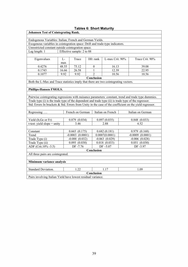
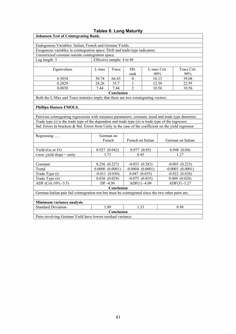
(i) Johansen Procedure: In Tables 6 , 8 and 9, it is clear that that there are two

cointegrating vectors among the three yields at the short, long and very long

25

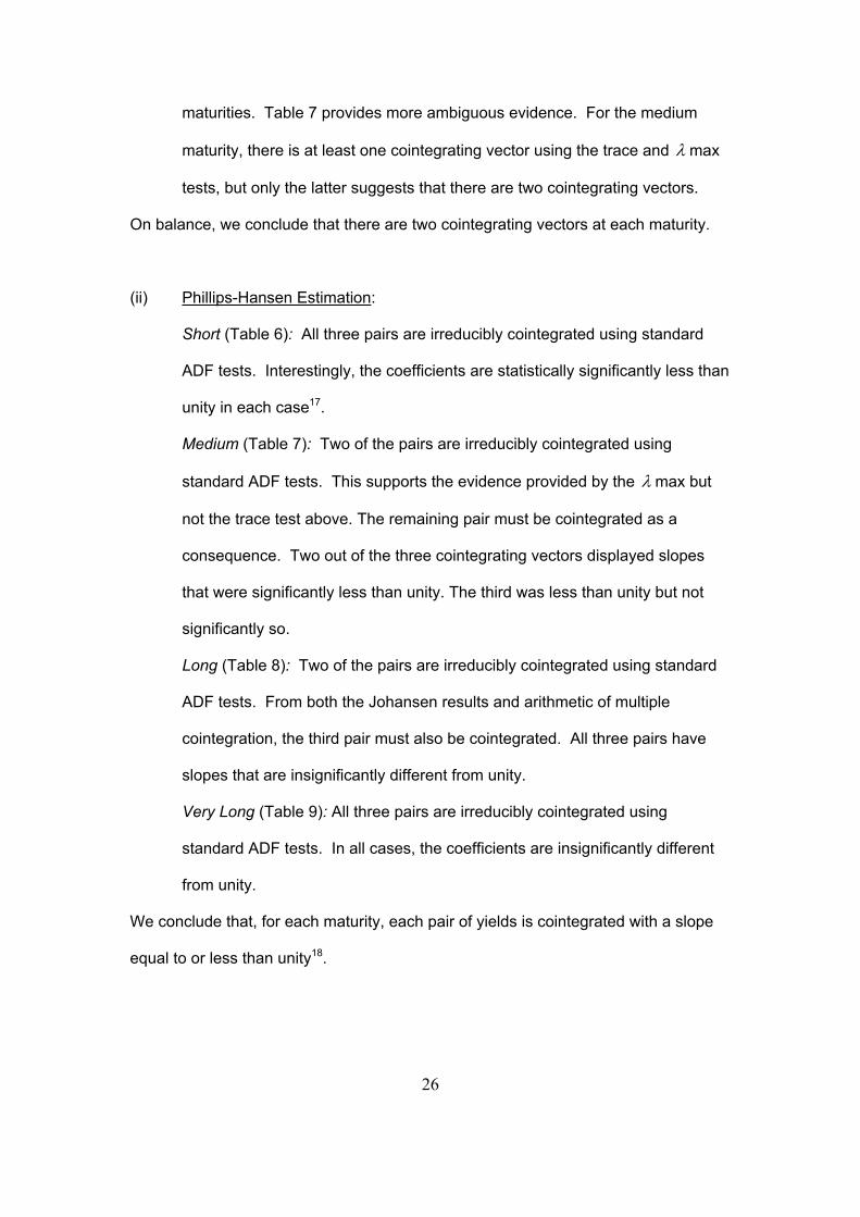
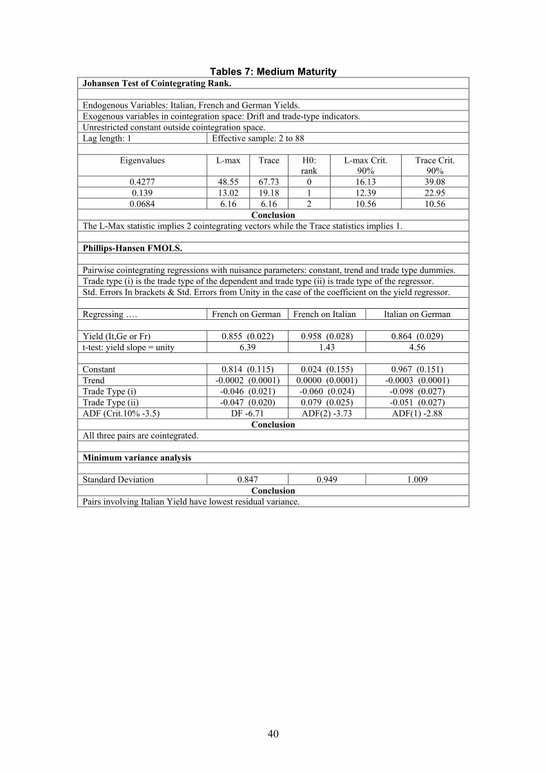
maturities. Table 7 provides more ambiguous evidence. For the medium

maturity, there is at least one cointegrating vector using the trace and λ max

tests, but only the latter suggests that there are two cointegrating vectors.

On balance, we conclude that there are two cointegrating vectors at each maturity.

(ii) Phillips-Hansen Estimation:

Short (Table 6): All three pairs are irreducibly cointegrated using standard

ADF tests. Interestingly, the coefficients are statistically significantly less than

unity in each case17.

Medium (Table 7): Two of the pairs are irreducibly cointegrated using

standard ADF tests. This supports the evidence provided by the λ max but

not the trace test above. The remaining pair must be cointegrated as a

consequence. Two out of the three cointegrating vectors displayed slopes

that were significantly less than unity. The third was less than unity but not

significantly so.

Long (Table 8): Two of the pairs are irreducibly cointegrated using standard

ADF tests. From both the Johansen results and arithmetic of multiple

cointegration, the third pair must also be cointegrated. All three pairs have

slopes that are insignificantly different from unity.

Very Long (Table 9): All three pairs are irreducibly cointegrated using

standard ADF tests. In all cases, the coefficients are insignificantly different

from unity.

We conclude that, for each maturity, each pair of yields is cointegrated with a slope

equal to or less than unity18.

26

(iii) BCH minimum variance ranking:

Short: The ranking of the variances of the residuals of the three cointegrating

vectors from smallest to largest is:

Italian-German

Italian-French

French-German

From this we conclude that that the Italian-German and Italian-French pairs

are structural and that the Italian yield provides the benchmark at the short

end.

Medium: The ranking of the variances of the residuals of the three

cointegrating vectors from smallest to largest is:

French-German

French-Italian

Italian-German

On this basis, the French yield is the benchmark at the medium maturity.

Long and Very Long: For both these maturities, the ranking of the variances

of the residuals of the three cointegrating vectors from smallest to largest is:

German-Italian

German-French

French-Italian

Thus the German market provides the benchmarks at both the long and very

long maturities.

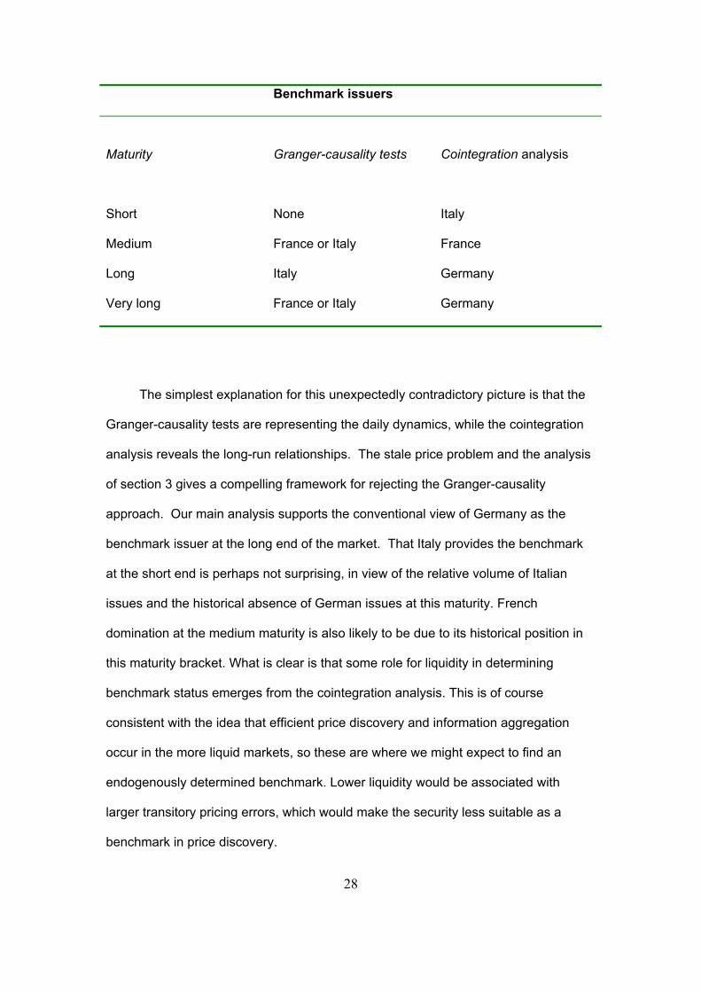
The results here contrast sharply with those based on Granger-causality, as

shown in this summary table:

27

Benchmark issuers

Maturity Granger-causality tests Cointegration analysis

Short None Italy

Medium France or Italy France

Long Italy Germany

Very long France or Italy Germany

The simplest explanation for this unexpectedly contradictory picture is that the

Granger-causality tests are representing the daily dynamics, while the cointegration

analysis reveals the long-run relationships. The stale price problem and the analysis

of section 3 gives a compelling framework for rejecting the Granger-causality

approach. Our main analysis supports the conventional view of Germany as the

benchmark issuer at the long end of the market. That Italy provides the benchmark

at the short end is perhaps not surprising, in view of the relative volume of Italian

issues and the historical absence of German issues at this maturity. French

domination at the medium maturity is also likely to be due to its historical position in

this maturity bracket. What is clear is that some role for liquidity in determining

benchmark status emerges from the cointegration analysis. This is of course

consistent with the idea that efficient price discovery and information aggregation

occur in the more liquid markets, so these are where we might expect to find an

endogenously determined benchmark. Lower liquidity would be associated with

larger transitory pricing errors, which would make the security less suitable as a

benchmark in price discovery.

28

5.3 Further interpretation of the cointegration results.

The factor-pricing model of section 2 was based on the idea of the benchmark

as a basket of bonds. In the analysis of section 5.2, we assumed that the property of

being a benchmark endogenously gravitated to one particular security. However, the

idea that the benchmark is a basket can be accommodated intuitively again at this

stage.

Consider the canonical case. If Germany were to provide the benchmark, we

expect that the yield gap between that country and each of France and Italy would be

stationary, mindful of the fact that all yields are non-stationary. Specifically, the

cointegrating vectors take the form:

Italian yield = α0 + α1German yield + stationary error (α1 = 1)

French yield = β0 + β1German yield + stationary error (β1 = 1)

From the Granger Representation Theorem (Engle and Granger, 1987), the

system has the following error correction representation:

∆Italian yield = λ0 + λ1(German/Italian yield gap) + λ2(German/French yield gap)

+ nuisance lags + noise

There are similar equations describing the evolution of the other yields.

29

The ECM equation above can be interpreted as follows: construct a portfolio

consisting of a long position in German bonds and an equal short position in Italian

bonds. Call this the first canonical benchmark portfolio. Its return equals the

German/Italian yield gap by construction. The parameter 1λ can be understood as

the loading sensitivity to that portfolio. A similar interpretation also applies to 2λ with

respect to a portfolio that is long in German bonds with an equal short position in

French bonds. Call this the second canonical benchmark portfolio.

In fact, however, we find that the two canonical portfolios constructed above

are not always the benchmark portfolios. Instead, we identify the benchmark

portfolios through estimation using the Phillips-Hansen FMOLS procedure. For

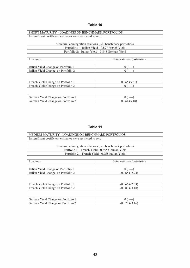
example, at the short maturity, the benchmark portfolios consist of

(i) a portfolio which is long in the Italian bond and (almost in equal measure)

short in the French bond

(ii) a portfolio which is long in the Italian bond and has an almost equal short

position in the German bond

The specific portfolios change depending on the structural relations chosen on

the basis of the cointegration analysis. As shown in Table 10, at the short maturity,

only the Italian-French portfolio (portfolio (i) above) is significant for French yields.

Similarly, only the Italian-German portfolio (portfolio (ii) above) is significant for

German yields. The Italian yield changes are not related to either portfolio, so that

the Italian yield is weakly exogenous - a likely property of a benchmark.

30

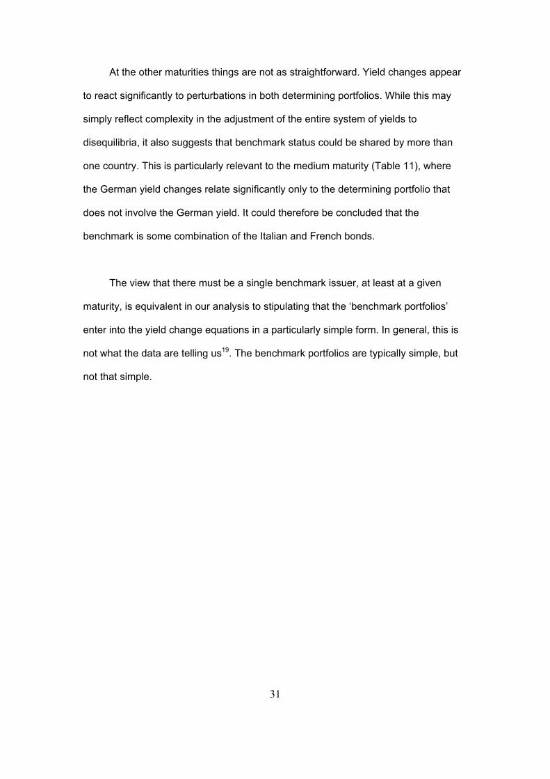
At the other maturities things are not as straightforward. Yield changes appear

to react significantly to perturbations in both determining portfolios. While this may

simply reflect complexity in the adjustment of the entire system of yields to

disequilibria, it also suggests that benchmark status could be shared by more than

one country. This is particularly relevant to the medium maturity (Table 11), where

the German yield changes relate significantly only to the determining portfolio that

does not involve the German yield. It could therefore be concluded that the

benchmark is some combination of the Italian and French bonds.

The view that there must be a single benchmark issuer, at least at a given

maturity, is equivalent in our analysis to stipulating that the ‘benchmark portfolios’

enter into the yield change equations in a particularly simple form. In general, this is

not what the data are telling us19. The benchmark portfolios are typically simple, but

not that simple.

31

6. Conclusion

We focus on the meaning of ‘benchmark’ bond in the context of the market for

euro-area government securities, extending the theoretical definition of a benchmark

in Yuan (2002). This market has developed rapidly since the beginning of monetary

union, but it is still not fully integrated, and there is no consensus20 regarding which

securities have benchmark status. We investigate two possible empirical criteria -

using Granger-causality and the Modified Davidson Method which uses

cointegration. We find rather different results with the two methods. The former

generates results which are either inconclusive or lack plausibility. The Modified

Davidson Method gives clear-cut results that are both plausible and congruent with

the theory that we present. But with neither do we find the unambiguous benchmark

status for German securities that would come from a simple focus on the securities

with lowest yield at a given maturity. Our interpretation of the cointegration results in

an error correction framework leads naturally to looking for benchmark portfolios

rather than a single benchmark security. This may be particularly appropriate in this

newly and only partially integrated market.

Clearly more research is needed, and the Euro-MTS database that we use is a

rich source. Meanwhile, however, we believe it is clear from the research reported

here that at least in the euro area, no simple definition of benchmark status will do.

Perhaps the markets are coming to understand this too:

‘German government bonds, long the unrivalled royalty of the European debt market, now find pretenders to the throne. The German government is careful…to protect the benchmark status of its bonds…But all the good intentions…are nothing in the face of the inexorable march of European monetary union. The euro-driven integration of European financial markets is creating vigorous competition to Germany’s long reign as king of the region’s bond markets. “Benchmark status is more contended now than it ever was,” said Adolf Rosenstock, European economist in Frankfurt at Nomura Research…’ (International Herald Tribune, 21 March 2002)

32

References Barassi, M. R., G. M. Caporale, and S. G. Hall, 2000a, Interest Rate Linkages: Identifying Structural Relations, Discussion Paper no. 2000.02, Centre for International Macroeconomics, University of Oxford. Barassi, M. R., G. M. Caporale, and S. G. Hall, 2000b, Irreducibility and Structural Cointegrating Relations: An Application to the G-7 Long Term Interest Rates, Working Paper ICMS4, Imperial College of Science, Technology and Medicine. Blanco, R., 2001, The euro-area government securities markets: recent developments and implications for market functioning, Working Paper no. 0120, Servicio de Estudios, Banco de Espana. Blanco, R., 2002, The euro-area government securities markets: recent developments and implications for market functioning, mimeo, Launching Workshop of the ECB-CFS Research Network on Capital Markets and Financial Integration in Europe, European Central Bank. Codogno, L., C. Favero, and A. Missale, 2003, Yield spreads on EMU government bonds, at www.economic-policy.org/pdfs/Preliminary_drafts/37thPanel_meeting/Codognoetal.pdf, forthcoming in Economic Policy October 2003. Davidson, J., 1998, Structural relations, cointegration and identification: some simple results and their application, Journal of Econometrics 87,87-113. Favero, C., A. Missale, and G. Piga, 2000, EMU and public debt management: one money, one debt?, CEPR Policy Paper No. 3. Galati, G., and K. Tsatsaronis, 2001, The impact of the euro on Europe’s financial markets, Working Paper No. 100, Bank for International Settlements. Engle, R.F., and C. W. J. Granger, 1987, Co-integration and error-correction: representation, estimation, and testing, Econometrica, 55, 1987, 251-76. Hasbrouck, J., One Security, Many Markets: Determining the Location of Price Discovery, Journal of Finance, 50, 4, 1995, 1175-1199 Lo, A., and A. C. MacKinlay, 1990, An Econometric Analysis of Nonsynchronous Trading, Journal of Econometrics, 45, 181-212. McCauley, R., 1999, The Euro and the Liquidity of European Fixed Income Markets, in Part 2.2. of “Market Liquidity: Research Findings and Selected Policy Implications", Committee on the Global Financial System, Bank for International Settlements, Publications No. 11 (May 1999). Portes, R., 2003, Discussion of Codogno et al., forthcoming in Economic Policy October 2003.

33

Remolona E. M., 2002, Micro and Macro structures in fixed income markets: The issues at stake in Europe, mimeo, Launching Workshop of the ECB-CFS Research Network on Capital Markets and Financial Integration in Europe, European Central Bank.

Scalia, A., and V. Vacca 1999, Does market transparency matter? a case study, Discussion Paper 359, Banca d’Italia. Sims, C., 1980, Macroeconomics and Reality. Econometrica 48 (1), 1-48. Yuan, K., (2002), The Liquidity Service of Sovereign Bonds, mimeo, University of Michigan Business School, available at http://webuser.bus.umich.edu/kyuan/exter_final.pdf

34

Figure 1

Source: Galati and Tsatsaronis (2001, p. 8)

Figure 2

Source: Blanco (2001, p. 31)

35

Table 1

Source: Galati and Tsatsaronis (2001, p. 7)

Table 2

Source: Blanco (2001, p. 23)

36

Table3

Source: Blanco (2001, p. 28)

Table 4

OVERVIEW OF THE COVERAGE OF THE DATA SET. Country Number

of Bonds.

% Number of Transactions

All Bonds.

% Transactions In Most liquid

bond.

%

Short Maturity. German 7 16.7 808 3.7 280 11.9 French 4 9.5 938 4.3 517 22.0 Italian 31 73.8 20151 92.0 1551 66.1

Medium Maturity. German 23 36.5 1358 4.9 407 6.0 French 11 17.5 2048 7.5 606 9.0 Italian 29 46.0 24046 87.6 5744 85.0

Long Maturity. German 20 43.5 2221 6.3 722 3.0 French 15 32.6 2426 6.8 1081 4.5 Italian 11 23.9 30873 86.9 22059 92.4

Very-Long Maturity. German 4 28.6 1127 13.5 679 12.2 French 5 35.7 451 5.4 261 4.7 Italian 5 35.7 6767 81.1 4641 83.2

All Maturities. Total Short 42 25.5 21897 23.5 2348 6.1

Total Medium 63 38.2 27452 29.5 6757 17.5 Total Long 46 27.9 35520 38.1 23862 61.9

Total V-Long 14 8.5 8345 9.0 5581 14.5 Total All 165 100.0 93214 100.0 38548 100.0

37

Table 5: Stationarity test results. SERIES Test t-value Conclusion

SHORT YIELD Italian ADF(1) 1.23 Non-stationary French DF -0.78 Non-stationary German DF -0.48 Non-stationary

MEDIUM YIELD Italian ADF(2) 1.605 Non-stationary French ADF(2) 0.48 Non-stationary German ADF(2) 0.842 Non-stationary

LONG YIELD Italian ADF(2) 1.67 Non-stationary French DF -0.134 Non-stationary German ADF(3) 0.3129 Non-stationary

V-LONG YIELD Italian DF -0.098 Non-stationary French DF 0.044 Non-stationary German DF -0.32 Non-stationary

SHORT YIELD-GAP Italian-German ADF(1) -0.97 Non-stationary French-German DF -6.27 Stationary Italian-French ADF(1) -1.81 Non-stationary

SHORT YIELD-GAP (with trend) Italian-German DF -4.32 Stationary French-German DF -7.29 Stationary Italian-French DF -5.57 Stationary

MEDIUM YIELD-GAP Italian-German ADF(1) -2.211 Non-stationary French-German DF -3.9165 Stationary Italian-French DF -3.8 Stationary

MEDIUM YIELD-GAP (with trend) Italian-German DF -2.45 Non-stationary French-German DF -3.86 Stationary Italian-French DF -4.4 Stationary

LONG YIELD-GAP Italian-German ADF(2) -1.529 Non-stationary French-German ADF(2) -3.147 Stationary Italian-French ADF(1) -2.905 Stationary

LONG YIELD-GAP(with trend) Italian-German ADF(3) -1.907 Non-stationary French-German DF -4.764 Stationary Italian-French DF -4.399 Stationary

V-LONG YIELD-GAP Italian-German ADF(2) -1.908 Non-stationary French-German DF -6.312 Stationary Italian-French ADF(1) -1.788 Non-stationary

V-LONG YIELD-GAP(with trend) Italian-German ADF(2) -2.24 Non-stationary French-German DF -6.71 Stationary Italian-French ADF(1) -2.179 Non-stationary

38

Tables 6: Short Maturity

Johansen Test of Cointegrating Rank. Endogenous Variables: Italian, French and German Yields. Exogenous variables in cointegration space: Drift and trade-type indicators. Unrestricted constant outside cointegration space. Lag length: 1 Effective sample: 2 to 88

Eigenvalues L-max

Trace H0: rank L-max Crit. 90% Trace Crit. 90%

0.4276 48.55 75.12 0 16.13 39.08 0.1743 16.66 26.58 1 12.39 22.95 0.1077 9.92 9.92 2 10.56 10.56

Conclusion Both the L-Max and Trace statistics imply that there are two cointegrating vectors. Phillips-Hansen FMOLS. Pairwise cointegrating regressions with nuisance parameters: constant, trend and trade type dummies. Trade type (i) is the trade type of the dependent and trade type (ii) is trade type of the regressor. Std. Errors In brackets & Std. Errors from Unity in the case of the coefficient on the yield regressor. Regressing …. French on German Italian on French Italian on German Yield (It,Ge or Fr) 0.879 (0.034) 0.897 (0.035) 0.848 (0.033) t-test: yield slope = unity 3.46 2.88 4.52 Constant 0.665 (0.175) 0.682 (0.181) 0.979 (0.168) Trend -0.0003 (0.0001) 0.0007(0.0001) -0.0009 (0.0001) Trade Type (i) -0.088 (0.032) -0.063 (0.029) -0.006 (0.028) Trade Type (ii) 0.095 (0.030) 0.018 (0.033) 0.051 (0.030) ADF (Crit.10% -3.5) DF -7.76 DF –5.07 DF -3.97

Conclusion All three pairs are cointegrated. Minimum variance analysis Standard Deviation. 1.22 1.17 1.09

Conclusion Pairs involving Italian Yield have lowest residual variance.

39

Tables 7: Medium Maturity Johansen Test of Cointegrating Rank. Endogenous Variables: Italian, French and German Yields. Exogenous variables in cointegration space: Drift and trade-type indicators. Unrestricted constant outside cointegration space. Lag length: 1 Effective sample: 2 to 88

Eigenvalues L-max Trace H0: rank

L-max Crit. 90%

Trace Crit. 90%

0.4277 48.55 67.73 0 16.13 39.08 0.139 13.02 19.18 1 12.39 22.95

0.0684 6.16 6.16 2 10.56 10.56 Conclusion

The L-Max statistic implies 2 cointegrating vectors while the Trace statistics implies 1. Phillips-Hansen FMOLS. Pairwise cointegrating regressions with nuisance parameters: constant, trend and trade type dummies. Trade type (i) is the trade type of the dependent and trade type (ii) is trade type of the regressor. Std. Errors In brackets & Std. Errors from Unity in the case of the coefficient on the yield regressor. Regressing …. French on German French on Italian Italian on German Yield (It,Ge or Fr) 0.855 (0.022) 0.958 (0.028) 0.864 (0.029) t-test: yield slope = unity 6.39 1.43 4.56 Constant 0.814 (0.115) 0.024 (0.155) 0.967 (0.151) Trend -0.0002 (0.0001) 0.0000 (0.0001) -0.0003 (0.0001) Trade Type (i) -0.046 (0.021) -0.060 (0.024) -0.098 (0.027) Trade Type (ii) -0.047 (0.020) 0.079 (0.025) -0.051 (0.027) ADF (Crit.10% -3.5) DF -6.71 ADF(2) -3.73 ADF(1) -2.88

Conclusion All three pairs are cointegrated. Minimum variance analysis

Standard Deviation 0.847 0.949 1.009

Conclusion Pairs involving Italian Yield have lowest residual variance.

40

Tables 8: Long Maturity Johansen Test of Cointegrating Rank. Endogenous Variables: Italian, French and German Yields. Exogenous variables in cointegration space: Drift and trade-type indicators. Unrestricted constant outside cointegration space. Lag length: 3 Effective sample: 4 to 88

Eigenvalues L-max Trace H0: rank

L-max Crit. 90%

Trace Crit. 90%

0.3034 30.74 66.43 0 16.13 39.08 0.2829 28.26 35.7 1 12.39 22.95 0.0838 7.44 7.44 2 10.56 10.56

Conclusion Both the L-Max and Trace statistics imply that there are two cointegrating vectors. Phillips-Hansen FMOLS. Pairwise cointegrating regressions with nuisance parameters: constant, trend and trade type dummies. Trade type (i) is the trade type of the dependent and trade type (ii) is trade type of the regressor. Std. Errors In brackets & Std. Errors from Unity in the case of the coefficient on the yield regressor. Regressing …. German on

French French on Italian German on Italian Yield (Ge or Fr) 0.927 (0.042) 0.977 (0.05) 0.948 (0.04) t-test: yield slope = unity 1.71 0.45 1.27 Constant 0.256 (0.227) -0.033 (0.283) -0.005 (0.225) Trend 0.0000 (0.0001) -0.0004 (0.0001) -0.0003 (0.0001) Trade Type (i) -0.011 (0.030) 0.047 (0.035) -0.022 (0.028) Trade Type (ii) 0.036 (0.029) -0.075 (0.035) 0.009 (0.028) ADF (Crit.10% -3.5) DF -4.50 ADF(1) -4.09 ADF(5) -3.27

Conclusion German-Italian pair fail cointegration test but must be cointegrated since the two other pairs are. Minimum variance analysis Standard Deviation 1.09 1.33 0.98

Conclusion Pairs involving German Yield have lowest residual variance.

41

Tables 9: Very-Long Maturity Johansen Test of Cointegrating Rank. Endogenous Variables: Italian, French and German Yields. Exogenous variables in cointegration space: Drift and trade-type indicators. Unrestricted constant outside cointegration space. Lag length: 1 Effective sample: 2 to 88

Eigenvalues L-max Trace H0: rank

L-max Crit. 90%

Trace Crit. 90%

0.4064 45.37 70.67 0 16.13 39.08 0.1726 16.48 25.3 1 12.39 22.95 0.0964 8.82 8.82 2 10.56 10.56

Conclusion Both the L-Max and Trace statistics imply that there are two cointegrating vectors. Phillips-Hansen FMOLS. Pairwise cointegrating regressions with nuisance parameters: constant, trend and trade type dummies. Trade type (i) is the trade type of the dependent and trade type (ii) is trade type of the regressor. Std. Errors In brackets & Std. Errors from Unity in the case of the coefficient on the yield regressor. Regressing …. German on

French French on Italian German on Italian Yield (It,Ge or Fr) 0.955 (0.028) 1.027 (0.057) 1.006 (0.054) t-test: yield slope = unity 1.56 0.47 0.12 Constant 0.150 (0.163) -0.398 (0.342) -0.372 (0.322) Trend 0.0000 (0.0001) -0.0004 (0.0001) -0.0003 (0.0001) Trade Type (i) -0.003 (0.023) 0.167 (0.043) -0.076 (0.040) Trade Type (ii) 0.032 (0.023) -0.001 (0.043) 0.043 (0.041) ADF (Crit.10% -3.5) DF -6.92 ADF(1) –3.62 DF -3.61

Conclusion All three pairs are cointegrated. Minimum variance analysis Standard Deviation 0.97 1.59 1.46

Conclusion Pairs involving German Yield have lowest residual variance.

42

Table 10 SHORT MATURITY - LOADINGS ON BENCHMARK PORTFOLIOS. Insignificant coefficient estimates were restricted to zero.

Structural cointegration relations (i.e., benchmark portfolios). Portfolio 1: Italian Yield - 0.897 French Yield Portfolio 2: Italian Yield - 0.848 German Yield

Loadings Point estimate (t-statistic) Italian Yield Change on Portfolio 1 0 ( ----) Italian Yield Change on Portfolio 2 0 ( ----)

French Yield Change on Portfolio 1 0.065 (5.31) French Yield Change on Portfolio 2 0 ( ----)

German Yield Change on Portfolio 1 0 ( ----) German Yield Change on Portfolio 2 0.064 (5.18)

Table 11 MEDIUM MATURITY - LOADINGS ON BENCHMARK PORTFOLIOS. Insignificant coefficient estimates were restricted to zero.

Structural cointegration relations (i.e., benchmark portfolios). Portfolio 1: French Yield - 0.855 German Yield Portfolio 2: French Yield - 0.958 Italian Yield

Loadings Point estimate (t-statistic) Italian Yield Change on Portfolio 1 0 ( ----) Italian Yield Change on Portfolio 2 -0.065 (-2.94)

French Yield Change on Portfolio 1 -0.066 (-2.33) French Yield Change on Portfolio 2 -0.083 (-3.18)

German Yield Change on Portfolio 1 0 ( ----) German Yield Change on Portfolio 2 -0.078 (-3.16)

43

Table 12

LONG MATURITY - LOADINGS ON BENCHMARK PORTFOLIOS. Insignificant coefficient estimates were restricted to zero.

Structural cointegration relations (i.e., benchmark portfolios). Portfolio 1: German Yield - 0.967 French Yield Portfolio 2: Italian Yield - 0.927 German Yield

Loadings Point estimate (t-statistic) Italian Yield Change on Portfolio 1 0 ( ----) Italian Yield Change on Portfolio 2 0.028 (2.01)

French Yield Change on Portfolio 1 0.040 (2.26) French Yield Change on Portfolio 2 0.056 (2.94)

German Yield Change on Portfolio 1 0 ( ----) German Yield Change on Portfolio 2 0.050 (3.15)

Table 13

VERY-LONG MATURITY - LOADINGS ON BENCHMARK PORTFOLIOS. Insignificant coefficient estimates were restricted to zero.

Structural cointegration relations (i.e., benchmark portfolios). Portfolio 1: German Yield - 0.955 French Yield Portfolio 2: Italian Yield - 0.967 German Yield

Loadings Point estimate (t-statistic) Italian Yield Change on Portfolio 1 0 ( ----) Italian Yield Change on Portfolio 2 0.021 (2.17)

French Yield Change on Portfolio 1 0.003 (2.14) French Yield Change on Portfolio 2 0.028 (2.61)

German Yield Change on Portfolio 1 -0.039 (-2.46) German Yield Change on Portfolio 2 0.035 (3.19)

44

45

Endnotes A web page which contains a number of more detailed results is referred to in a number of the endnotes below. The address is http://qub-recon.vhost.tibus.com/uploads/Web_Appendix.doc 1 See Blanco (2002). 2 Descriptive statistics are available from the relevant web page listed above. 3 It is essential to make this assumption because bond yields are typically non-atationary. 4 Ireland joined Euro-MTS in June 2002. 5 There is also a fifth category for bills: securities with maturity less than 1.25 years. However, until recently, only Italy was significantly trading such instruments on Euro-MTS. 6 We are grateful to Rich Lyons and Kathy Yuan for pointing out that there may be a “stale price” problem that incorrectly manifests as Granger Causality. This casts further doubt on the usefulness of Granger Causality as a means to identify the benchmark. 7 We use 12.30 as the end of the morning trading period and 4.30 as the end of the afternoon trading period. 8 The Granger causality results are discussed in the next section. 9 Available at the relevant web page listed above. 10 More details of these tests can be obtained from the relevant web address listed above. 11 Details of the lag-length selection can be found on the relevant web page listed above. 12 Granger causality results are summarised in the Table at the end of section 5.2 and further details are available in the web appendix. 13 A strong restriction is that the constant in both cointegrating vectors be unity. This corresponds to two stationary yield gaps. We already know from the discussion in Section 3 that this is problematic. 14 If residuals from the structural vectors are not orthogonal, then it is not clear what ‘structural’ means in this context. It is essential one way or the other to make some assumption about the covariance between the structural relations. However, any assumption other than a zero value makes the application of the irreducible cointegrating vector approach inconclusive.

15 It is easy to show that 2 13 and e ee γδ

β β−

= =

16 In two instances in the very-long maturity the point estimate for what could be referred to as γ is above unity but is not statistically significantly so. 17 To see this, we report a fully modified t-test that tests for the difference between the estimated coefficient and unity. In each of Tables 6 to 9, this is shown in the row labelled “t-test: yield slope = unity”. 18 The Phillips-Hansen approach is a least squares technique so that in small samples, results depend on which variable is selected as the dependent variable. We carried out the above estimation and testing procedure for each pair in each of the two possible variants. We selected the reported result on the basis of the one that had the lowest residual variance. 19 The results for the long and very-long maturities are shown in Tables 12 and 13. 20 Remolona (2002) argues that the swaps market now provides the benchmark yield curve for euro denominated bonds.