DEFINITION OF BOUNDARY AND INITIAL CONDITIONS · PDF fileof the United States Geological...

Techniques of Water-Resources Investigations

of the United States Geological Survey

Chapter B5

DEFINITION OF BOUNDARY AND INITIAL CONDITIONS IN THE ANALYSIS OF SATURATED GROUND-WATER FLOW

SYSTEMS-AN INTRODUCTION

By 0. Lehn Franke, Thomas E. Reilly, and Gordon D. Bennett

Book 3

APPLICATIONS OF HYDRAULICS

http://www.usgs.gov

njestes

Click here to return to USGS publications

../index.html

DEPARTMENT OF THE INTERIOR

DONALD PAUL HODEL, Secretary

U.S. GEOLOGICAL SURVEY

Dallas 1. Peck, Director

UNITED STATES GOVERNMENT PRINTING OFFICE, WASHINGTON : 1987

For sale by the Books and Open-File Reports Section, U.S. Geological Survey, Federal Center, Box 25425, Denver, CO 80225

PREFACE

The series of manuals on techniques describes procedures for planning and executing specialized work in water-resources investigations. The material is grouped under major subject headings called books and further subdivided into sections and chapters; section B of book 3 is on ground-water techniques.

The unit of publication, the chapter, is limited to a narrow field of subject matter. This format permits flexibility in revision and publication as the need arises. Chapter 3B5 deals with the definition of boundary and initial conditions in the analysis of saturated ground-water flow systems.

Provisional drafts of chapters are distributed to field offices of the U.S. Geological Survey for their use. These drafts are subject to revision because of experience in use or because of advancement in knowledge, techniques, or equipment. After the technique described in a chapter is sufficiently developed, the chapter is published and is for sale from U.S. Geological Survey, Books and Open-File Reports Section, Federal Center, Box 25425, Denver, CO 80225.

Reference to trade names, commercial products, manufacturers, or distributors in this manual constitutes neither endorsement by the Geological Survey nor recommen- dation for use.

III

TECHNIQUES OF WATER-RESOURCES INVESTIGATIONS OF THE UNITED STATES GEOLOGICAL SURVEY

The U.S. Geological Survey publishes a series of manuals describing procedures for planning and conducting specialized work in water-resources investigations. The manuals published to date are listed below and may be ordered by mail from the U.S. Geological Survey, Books and Open-File Reports, Federal Center, Box 25425, Denwq Colorado 80225 an authorized agent of the Superintendent of Documents, Government Printing Office).

Prepayment is required. Remittance should be sent by check or money order payable to U.S. Geological Survey. Prices are not included in the listing below as they are subject to change. Current prices can be obtained by writing to the USGS, Books and Open File Reports. Prices include cost of domestic surface transportation. For transmittal outside the U.S.A. (except to Canada and Mexico) a surcharge of 25 percent of the net bill should be included to cover surface transportation. When ordering any of these publications, please give the title, book number, chapter number, and “U.S. Geological Survey Techniques of Water-Resources Investigations.”

TWI 1-Dl.

TWI l-D2.

TWI 2-Dl. TWI 2-El. TWI 3-Al. TWI 3-A2. Tw 3-A3. TWI 3-A4. TWI 3-A5. TWI 3-A6. TWI 3-A7. TWI 3-A8. TWI 3-A9.

Water temperature-influential factors, field measurement, and data presentation, by H.H. Stevens, Jr., J.F. Ficke, and G.F. Smoot, 1975, 65 pages.

Guidelines for collection and field analysis of ground-water samples for selected unstable constituents, by W.W. Wood. 1976. 24 pages.

Application of surface geophysics to ground water investigations, by A.A.R. Zohdy, G.P. Eaton, and D.R. Mabey. 1974. 116 pages. Application of borehoie geophysics to water-resources investigations, by W.S. Keys and L.M. MacCary. 1971. 126 pages. General field and office procedures for indirect discharge measurement, by M.A. Benson and Tate Dahymple. 1967. 30 pages. Measurement of peak discharge by the slope-area method, by Tate Dalrymple and M.A. Benson. 1967. 12 pages. Measurement of peak discharge at culverts by indirect methods, by G.L. Bodhaine. 1968. 60 pages. Measurement of peak discharge at width contractions by indirect methods, by H.F. Matthai. 1967. 44 pages. Measurement of peak discharge at dams by indirect methods, by Harty Hulsing. 1967. 29 pages. General procedure for gaging streams, by R.W. Carter and Jacob Davidian. 1968. 13 pages. Stage measurements at gaging stations, by T.J. Buchanan and W.P. Somers. 1968. 28 pages. Discharge measurements at gaging stations, by T.J. Buchanan and W.P. Somers. 1969. 65 pages. Measurement of time of travel and dispersion in streams by dye tracing, by E.P. Hubbard, F.A. Kilpatrick, L.A. Martens, and

J.F. Wilson, Jr. 1982. 44 pages. TWI 3-AlO. Discharge ratings at gaging stations, by E.J. Kennedy. 1984. 59 pages. TWI 3-All. Measurement of discharge by moving-boat method, by G.F. Smoot and C.C. Novak. 1969. 22 pages. TWI 3-A12. Fiuorometric procedures for dye tracing, Revised, by James F. Wilson, Jr., Ernest D. Cobb, and Frederick A. Kilpatrick. 1986. 41

pages TWI 3-A13. Computation of continuous records of streamflow, by Edward J. Kennedy. 1983.53 pages. TWI 3-A14. Use of flumes in measuring discharge, by F.A. Kilpatrick, and V.R. Schneider. 1983. 46 pages. TWI 3-A15 Computation of water-surface profiles in open channels, by Jacob Davidian. 1984. 48 pages. TWI 3-A16. Measurement of discharge using tracers, by F.A. Kilpatrick and E.D. Cobb. 1985. 52 pages. TWI 3-A17. Acoustic velocity me&r systems, by Antonius Laenen. 1985. 38 pages. TWI 3-Bl. Aquifer-test design, observation, and data analysis, by R.W. Stallman. 1971. 26 pages. TWI 3-B2. Introduction to ground-water hydraulics, a programmed text for self-instruction, by G.D. Bennett. 1976. 172 pages. Spanish

translation TWI 3-B2 also available. TWI 3-B3. Type curves for selected problems of flow to wells in confined aquifers, by J.E. Reed. 1980. 106 p. TWI 3-B6. The principle of superposition and its application in ground-water hydraulics, by Thomas E. Reilly, 0. Lehn Franke, and Gordon D.

Bennett. 1987. 28 pages. TWI 3X1. Fiuvial sediment concepts, by H.P. Guy. 1970. 55 pages. TWI 3X2. Field methods of measurement of Ruvial sediment, by H.P. Guy and V.W. Norman. 1970. 59 pages. TWI 3X3. Computation of fluvial-sediment discharge, by George Porterfield. 1972. 66 pages. TWI 4-Al. Some statistical tools in hydrology, by H.C. Riggs. 1968. 39 pages. TWI 4-A2. Frequency cmves, by H.C. Riggs, 1968. 15 pages. TWI 4-Bl. Low-flow investigations, by H.C. Riggs. 1972. 18 pages. TWI 4-B2. Storage analyses for water supply, by H.C. Riggs and C.H. Hardison. 1973. 20 pages. TWI 4-B3. Regional anaiyses of streamflow characteristics, by H.C. Riggs. 1973. 15 pages. TWI 4-Dl. Computation of rate and volume of stream depletion by wells, by C.T. Jenkins. 1970. 17 pages. TWI S-Al. Methods for determination of inorganic substances in water and fiuvial sediments, by M.W. Skougstad and others, editors. 1979. 626

pages- TWI 5-A2. Determination of minor elements in water by emission spectroscopy, by P.R. Bamett and E.C. Mallory, Jr. 1971. 31 pages.

N

TWI 543.

0 TWI S-A4.

TWI 5-A%

TWI .5-A6.

TWI S-Cl. TWI 7x1.

TWI 7X2.

TWI 7x3.

l-w 8-Al. Methods of measuring water levels in deep wells, by M.S. Garber and EC. Koopman. 1968. 23 pages. TWI 8X2. Installation and service manual for U.S. Geological Survey monometers, by J.D. Craig. 1983. 57 pages. TWI 8-B2. Calibration and maintenance of vertical-axis type current meters, by G.F. Smoot and C.E. Novak. 1968. 15 pages.

Methods for the determination of organic substances in water and fluvial sediments, edited by R.L. Wershaw, M.J. Fishman, R.R. Grabbe, and L.E. Lowe. 1987. 80 pages. This manual is a revision of “Methods for Analysis of Organic Substances in Water” by Donald F. Goerlitz and Eugene Brown, Book 5, Chapter A3, published in 1972.

Methods for collection and analysis of aquatic biological and microbiological samples, edited by P.E. Greeson, T.A. Ehike, G.A. Irwin, B.W. Lium, and K.V. Slack. 1977. 332 pages.

Methods for determination of radioactive substances in water and fluvial sediments, by L.L. Thatcher, VJ. Janzer, and KW. Edwards. 1977.95 pages.

Quality assurance practices for the chemical and biological analyses of water and fluvial sediments, by L.C. Friedman and D.E. Erdmann. 1982. 181 pages.

Laboratory theory and methods for sediment analysis, by H.P. Guy. 1969. 58 pages. Finite difference model for aquifer simulation in two dimensions with results of numerical experiments, by PC. Trescott, G.F.

Pinder, and S.P. Larson. 1976. 116 pages. Computer model of two-dimensional solute transport and dispersion in ground water, by L.F. Konikow and J.D. Bredehoeft. 1978.

90 pages. A model for simulation of flow in singular and interconnected channels, by R.W. Schaffranek, R.A. Baltzer, and D.E. Goldberg.

1981. 110 pages.

CONTENTS

Page Abstract ________________________________________------------------------------------------------------------------------------ 1

Intr&uction ____-----___________-------------------------------------------------------------------------------------------- 1

Boundary conditions ___________-_--_________________________-------------------------------------------------------------- 1

principal types of boundav conditions ______________-___-_____________________--------------------------------- 2 Some important aspects of specifying boundary conditions in ground-water models --------------- 6

Model boun&&s versus physical boundaries ________________________________________------------------ 6 Selection of boundary conditions in relation to system stress -------------------------------------- 8 bun&q conditions in steady-state m&c& _-_-____-___--__---_---------------------------------------- 8 me water table as a boundq ________________________________________------------------------------------- 9 Reference elevation in ground-water models ________________________________________------------------- 9

&n&ding remarks ________________________________________-------------------------------------------------------- 10 J&r&es ________________________________________---------------------------------------------------------------------- 10

Initial conditions ___---__-_______________________________------------------------------------------------------------------ 10 Concept of initial conditions ________________________________________--------------------------------------------- 11 Specifying initial conditions in mo&ls ______-__--_-__-____---------------------------------------------------- 11 Eample of specifying initial conditions in a field situation -_______________________________________------ 12 &n&ding remarks ________________________________________----------------------------------------------.--------- 12

A&now]edgments ________________________________________---------------------------------------------------------------- 13 References ________________________________________------------------------------------------------------------------------- 13 Appendix: Discussion of the solution of differential equations and the role of boundary

conditions -_-------_-__--________________.__-__-_________________________________-------------------------------.----- 14

FIGURES

1. Flow net within three different hydraulic settings: Through and beneath an earth dam underlain by sloping bedrock; beneath a vertical impermeable wall; and beneath an impermeable dam and a vertical impermeable wall -------------------------------------------- 3

2-7. Diagrams of: 2. Piezometers at different depths demonstrating that the total head at all depths in a continuous body of stationary fluid is

constant------------------------------------------------------------------------------------------------------------------------------------------------------ 3 3. Plow pattern in uniformly permeable material with constant area1 recharge and discharge to symmetrically placed streams-------- 4 4. A leaky aquifer system ____________----__----------------------------------------------------------------------------------------------------------------------- 5 5. FQw pattern in a permeable dam having v&Cal faces ________________________________________-------------------------------------------------------- 7 6. flow pattern near a discharging well in an unconfined aquifer ________________________________________---------------------------------------------- 7 7. flow pattern near a ~awater-f~shwater interface ________________________________________------------------------------------------------------------- 8

8. Hydrograph of well N1614 tapping the upper glacial aquifer in central Nassau County, New York --------------------------------------------- 12 9. Example of solutions to a differential equation: Diagram of idealized aquifer system, and two of the family of curves solving the

general differential equation for the i&al&d aquifer system ____________________------------------------------------------------------------------- 15

TABLE

1. Common designations for several important boundary conditions ________________________________________--------------------------------------- - ------ -- 6

VIII CONTENTS

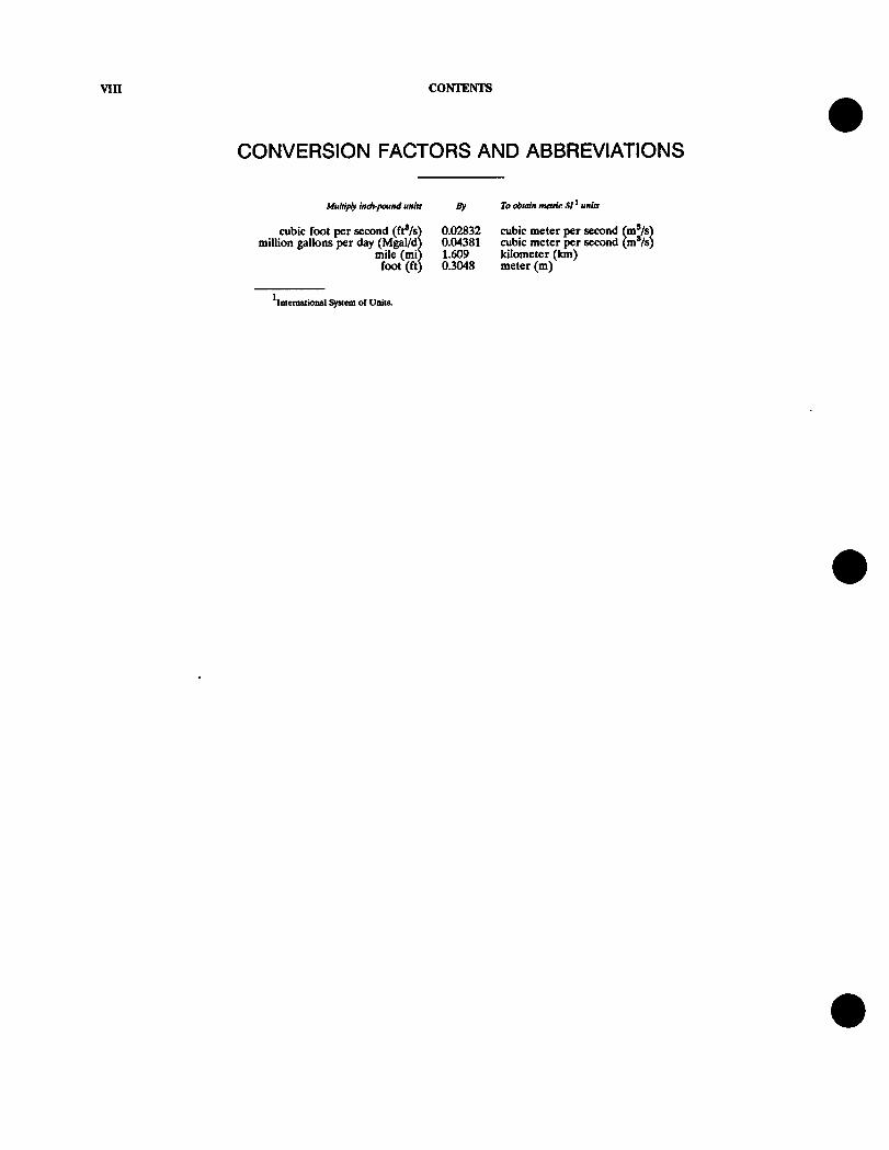
CONVERSION FACTORS AND ABBREVIATIONS

Muldply indt-pamd units 4 To dmdn otmie Sl'unirr

0.02832 cubic meter per second million gallons per 0.04381 cubic meter per second

::g8 kilometer (km) meter (m)

1 1ntemtioMl system of units.

DEFINITION OF BOUNDARY AND INITIAL CONDITIONS IN THE ANALYSIS OF SATURATED GROUND-WATER FLOW

SYSTEMS-AN INTRODUCTION

BJJ 0. Lehn Franke, Thomas E. Reilly, and Gordon D. Bennett

Abstract

Accurate definition of boundary and initial conditions is an essential part of conceptualizing and modeling ground-water flow systems. This report describes the properties of the seven most common boundary conditions encountered in ground-water systems and discusses major aspects of their application. It also discusses the significance and specification of initial conditions and evaluatessome common errors in applying this concept to ground-water-system models. An appendix is included that discusses what the solution of a differential equation represents and how the solution relates to the boundary conditions defining the specific problem. This report considers only boundary conditions that apply to saturated ground-water systems

Introduction The specification of appropriate boundary and initial

conditions is an essential part of conceptualizing and modeling1 ground-water systems and is also the part most subject to serious error by ground-water hydrologists. Although some excellent discussions of these topics are provided in a few readily available texts (for example, Bear, 1979, p. 94-102, 116-123; and Rushton and Redshaw,

‘The word “model” is used in several different ways in this report and in ground-water hydrology. A general definition of model is a representation of some or all of the properties of a system. Developing a “conceptual model” of the ground-water system is the first and critical step in any study, particularly studies involving mathematical- numerical modeling In this context, a conceptual model is a clear, qualitative, physical description of the operation of the natural system. A “mathematical model” represents the system under study through mathematical equations and procedures. The differential equations that describe in approximate terms a physical process (for example, ground-water flow and solute transport) are a mathematical model of that process. The solution to these differential equations in a specific problem frequently requires numerical procedures (algorithms), although many simpler mathematical models can be solved analytically. Thus the process of “modeling” usually implies developing either a conceptual model, a mathematical model, or a mathematical-numerical model of the system or problem under study. The context will suggest which meaning of “model” is intended.

1979, p. 153-156, 182-X44), most standard texts on ground-water hydrology do not thoroughly discuss these topics from the standpoint of ground-water flow modeling.

The purpose of this report is to provide a concise introduction to these topics to give ground-water hydrologists the information necessary to successfully apply these concepts in conceptualizing ground-water systems for the purpose of modeling.

The report consists of three parts. The first part provides the definition and properties of the most common boundary conditions in ground-water systems and discusses their application in special situations. The second part explains the concept of initial conditions and discusses some common pitfalls in specifying initial conditions in models of ground-water systems. The third part is an appendix that discusses what the solution of a differential equation represents and how the solution relates to the boundary conditions defining the specific problem. The report considers only boundary conditions that apply to saturated ground-water systems.

Boundary Conditions Quantitative modeling of a ground-water system entails

the solution of a boundary-value problem-a type of mathematical problem that has been extensively studied and has applications in many areas of science and tech- nology. The flow of ground water is described in the general case by partial differential equations. A ground- water problem is “defined” by establishing the appropriate boundary-value problem; solving the problem involves solving the governing partial differential equation in the flow domain while at the same time satisfying the specified boundary and initial conditions. In ground-water problems, the solution is usually expressed in terms of head (h); that is, head is usually the dependent variable in the governing partial differential equation. The solution to a simple boundary-value problem in ground-water flow is

1

2 TECHNIQUES OF WATER-RESOURCES INVESI-IGATIONS

given in the appendix and serves as an example of a formal solution to this type of problem.

Defining a specific ground-water problem in prepara- tion for subsequent quantitative modeling requires a clear concept of how the ground-water flow system under study functions. Various representations of a ground-water fknv system are possible, depending on one’s objectives and point of view. In this discussion, the term “flow system” refers to the part of the ground-water regime that has been isolated for study and implies the follawing: 1. A three-dimensional body of earth material is satu-

rated with fkxving ground water; 2. The region containing the ground water is bounded by

a closed surface called the “boundary surface” of the flow system;

3. Under natural (unstressed) conditions, average flow in the system, as well as average ground-water levels, normally fluctuate around a mean value;

4. Inflow (continuous or intermittent) of water to the system and outflow from it occur through at least part of the boundary surface.

In ground-water investigations, the system or subsystem under study ideally should be encbsed by a boundary surface that corresponds to identifiable hydrogeologic features at which some characteristic of ground-water flow is easily described; examples are a body of surface water, an almost impermeable surface, a water table, and so on. In many studies, however, some part of the boundary surface must be chosen arbitrarily, often in ways that depend on the proposed modeling strategy. The position of the three-dimensional boundary surface in nature (regardless of the extent to which it has been arbitrarily specified) defines the “external geometry” of the ground- water flow system.

Specifying the boundary conditions of the ground-water flow system means assigning a boundary type (usually one or a combination of the types listed in the following paragraphs) to every point on the boundary surface.

The selection of the boundary surface and boundary conditions is probably the most critical step in conceptualizing and developing a model of a ground-water system. Improper selection of these components may result in a failure of the modeling effort, with the result that the model’s response to an applied stress bears little relation to the corresponding response in the real system.

Usually the selection of boundary conditions for a conceptual or numerical model involves considerable sim- plification of actual hydrogeologic conditions. To avoid serious error, the assumptions underlying such simplifica- tions must be clearly understood and their effect on model response critically evaluated.

Principal types of boundary conditions

This section describes the pertinent characteristics of seven types of boundaries-constant head, specified head,

streamline (or stream surface), specified flux, head- dependent flux, free surface, and seepage surface.

1. Constant-head (surfixe or line) bounda~ -Hydraulic head (h) in a ground-water system is the sum of elevation head (z) and pressure head (ply), where p is gage pressure and y is the unit weight of water. Elevation head represents the potential energy of a water particle due to its vertical position above some datum, and pressure head represents pressure measured in terms of the height of a column of water in a piezometer. Physically, hydraulic head represents the water level above datum in a piezometer or observation well open only to the point in question.

A surface of equal head is an imaginary surface having the same head value at all points. Thus, all piezometers open to different points on a surface of equal head will show exactly the same water level in reference to a common datum. In a two-dimensional problemz, the concept of a line (rather than a curving surface) of equal head is used-that is, a line alongwhich all points have the same head value.

A constant-head boundary3 occurs where a part of the boundary surface of an aquifer system coincides with a surface of essentially constant head. (The word “constant,” as used here, implies a value that is uniform at all points along the surface as well as through time.) An example is an aquifer that crops out beneath a lake in which the surface-water stage is nearly uniform over all points of the outcrop and does not vary appreciably with time. Other examples of a constant-head boundary are shown in figure 1A (lines ABC, EG), figure lB (lines BA, CD), and figure 1C (lines AB, CD), all of which depict two-dimensional steady-state ground-water seepage beneath engineering structures that are bounded in part by surface-water bodies. The artificial lateral boundaries in figure 1 (dashed) are discussed later in the section “Model Boundaries Versus Physical Boundaries.”

Let us consider the boundary ABC in figure 1A. The question sometimes arises as to whether line BC on the submerged side of the dam in fact represents a uniform constant head (or constant potential) along its entire length. Obviously, thepressure varies with depth abng this surface. We assume that the surface water behind the dam is essentially static; the rule is that within such a body of stationary fluid, the total head is a constant at every point, including points along the boundary surface between the fluid body and the ground-water system, regardless of the surface configuration. To demonstrate this concept, consider piezometers at various depths in the body of a

a In a two-dimensional problem, the components of ground-water- velocity vectors can be designated by hvo coordinate axes. Two- dimensional flow is planar. The illustrations in this report depict two-dimensional problems; that is, ground-water flows only in the plane of the illustration.

sAlso referred to as constant-potential or equipotential boundary.

DEFINITION OF BOUNDARY AND INITIAL CONDITIONS 3

Impermeable layer (Bedrock)

ermeable dam

Impermeable wall Equwmtential line

c

Figure l.-Flow net within three different hydraulic settings: A, through and beneath an earth dam underlain by sloping bedrock; 6, beneath a vertical impermeable wall; and C, beneath an impermeable dam and a vertical impermeable wall.

stationary fluid (fig. 2). At the surface of the fluid body (piezometer A), where the fluid is in contact with the atmosphere, h =z because p/T =O. As one moves the piezometer downward from the fluid surface (piezometers B and C), the increase in pressure head (ply) is exactly balanced by a decrease in elevation head (z); thus, h remains constant.

2. Specified-head boundmy.-A more general type of boundary condition, of which the constant-head boundary is actually a special case, occurs wherever head can be specified as a function of position and time over a part of

Plezometers

I ” z C z=o

Body of stationary fluld (Datum)

Figure P.-Piezometers at different depths demonstrating that the total head at all depths in a continuous body of stationary fluid is constant.

the boundary surface of a ground-water system. An example of the simplest type might be an aquifer that is exposed along the bottom of a large stream whose stage is independent of ground-water seepage. As one moves upstream or downstream, the head changes in relation to the slope of the stream channel. If changes in head with time are not significant, the head can be specified as a function of position alone (h = f(x,y) in a two-dimensional analysis) at all points along the streambed. In a more complex situation, in which stream stage varies with time, head at points along the streambed would be specified as a function of both position and time, h = f(x,y,t). In either example, heads along the streambed are specified accord- ing to circumstances external to the ground-water system and maintain these specified values throughout the problem solution, regardless of the stresses to which the ground-water system is subjected.

Both specified-head and constant-head boundaries (or nodes, in a discretized analysis) have an important “physical” characteristic in models of ground-water systems-in effect, they can provide an inexhaustible source of water. No matter how much water is “pumped” from a system model, the specified-head boundaries will continue to supply the required amount, even if that amount is not physically reasonable in the real system. This aspect of specified-head boundaries should be considered carefully whenever this boundary type is selected for simulation and also when any model result or prediction is evaluated.

3. Streamline or stream-surface boundmy (no-flow).-A streamline is a curve that is tangent to the flow-velocity vector at every point along its length; thus, no flow components exist normal to a streamline and no flow crosses a streamline. Because a stream surface is a continuous three-dimensional surface made up entirely of streamlines, it follows that no flow crosses a stream

4 TECHNIQUES OF WATER-RESOURCES INVESl-fGATIONS

Equipotentlal ~meJ

Figure 3.-Flow pattern in uniformly permeable material with constant areal recharge and discharge to symmetrically placed streams. (Modified from Hubbett, 1940.)

surface. In a steady flow, that is, a flow that does not change with time, streamlines and stream surfaces remain constant, whereas in nonsteady or transient flow-flow that changes with time-the streamlines and stream surfaces in the interior of the flow may differ from one instant to the next. Even in nonsteady flows, however, it is common for some parts of the boundary to consist of stream surfaces that remain fixed with time. An example is an impermeable boundary. Natural earth materials are never completely impermeable. However they may sometimes be regarded as effectively impermeable for modeling pur- poses if the hydraulic conductivities of the adjacent materials differ by several orders of magnitude.

For an isotropic medium, the flow per unit area from a boundary into an aquifer is given by Darcy’s law4 as

ah q =-Kz,

where q is specific discharge (L/T), K is hydraulic conductivity of the aquifer (L/T), h is hydraulic head (L), and n is distance normal to the boundary (L).

The condition that q be equal to zero, as required for no-flow boundaries, can be satislkl only if ah/&r, the head gradient normal to the boundary, is also zero. Thus, a simple formulation of the no-flow condition in terms of head is possible.

An example of a boundary that is effectively impermeable is the contact between unweathered granite and permeable unconsolidated material; another is a sub-

‘ Hydraulic conductivity in the example above is specified as isotropic to simplify the form of Darcy’s law that is used. In anisotropic systems, the direction normal to the boundary (designated n) must coincide with a major axis of the hydraulic-conductivity tensor (represented geometrically by the hydraulic conductivity ellipsoid) to enable use of the simple form of Darcy’s law above in each coordinate direction. Otherwise, the off-diagonal terms of the hydraulicconductivity tensor are not zero and must be used to calculate the flus in the specified coordinate direction (Lehman and others 1972).

merged sheetpile walls. Some examples of boundaries that are assumed to be no-flow (stream-surface) boundaries l are depicted in figure 1/l, line HI; figure lB, lines AEC, FG; and figure lC, lines BGHC, EF.

4. Specified-fib boundary.-Another general type of boundary, of which the stream-surface (or no-flow) boundary is a special case, is found wherever the flux across a given part of the boundary surface can be specified as a function of position and time. (The term “flux” as used in this discussion refers to the volume of fluid crossing a unit cross-sectional surface area per unit time.) In the simplest type of specified-flux boundary, the flux across a given part of the boundary surface is considered uniform in space and constant with time; this assumption is often ma&, for example, with respect to area1 recharge crossing the upper surface of an aquifer A flow net depicting constant area1 recharge to a water table is shown in figure 3. Boundaries of this type are termed “constant-flux” boundaries, and the stream-surface boundary can be considered a special case in which the constant flux is zero. In a more general case, the flux might be constant with time but specified as a function of position: q = f(x,y,z) over the part of the boundary surface in question. In the most general case, flux is specified as a function of time as well as position: q = f(x,yJ,t).

In all three examples, fhrx across the boundary is specified-that is, it is established in advance and is not affected by events within the ground-water system; more- over, it may not deviate from its specified values during problem solution.

If the direction normal to the boundary coincides with a major axis of hydraulic. conductivity, the expression obtained above for flux from the boundary, q =-K,,(ah/an), can be used to provide a statement of the boundary condition in terms of head. Wr the constant-flux boundary we hme ah/an =constant, and for the two more general cases we have ah/&r=f(x,y,z) and ah/an = f(x,y,z,t), respectively.

5. Head-akpendent flip boundmy.-In some situations, flw across a part of the boundary surface changes in response to changes in head within the aquifer adjacent to the boundary. In these situations, the flux is a specified function of that head and varies during problem solution as the head varies. An example of this type of boundary is the upper surface of an aquifer overlain by a semiconfining bed that is in turn overlain by a body of surface water. This type of boundary is illustrated by line BC in figure 4. The head in the surface-water body remains constant, and the

s A continuous wall of driven piles, generally made of thick planks or corrugated sheet steel.


flux, q, across the semiconfining bed is given by Darcy’s law as

where K’ is the hydraulic conductivity of the semiconfin-

ing bed; b’ is its thickness; H is the head in the surface-water body, and h is the head in the aquifer.

Thus, flux is a linear function of head in the aquifer-as head falls, flux across the semiconfining bed increases, and as head rises, flux decreases.

Inherent in most head-dependent boundary situations is a practical limit beyond which changes in head cease to cause changes in flux. In the example cited above, this limit will be reached where the head within the aquifer falls below the top of the aquifer, so that the aquifer is no longer confined at that point, but rather is locally under an unconfined or water-table condition, while the semiconfining unit above remains saturated from top to bottom. Under these conditions, the bottom of the semiconfining bed becomes bcally a seepage face (discussed later) in the sense that it responds to atmospheric pressure in the unsaturated aquifer immediately beneath it. Thus, with atmospheric pressure considered to be zero, the head at the base of the semiconfining unit is simply the elevation (zJ of that point above datum, and no matter how much additional drawdown now occurs in the underlying aquifer, the flux through the semicontining bed remains constant, as given by

q ,H-z, =-K b, .

Thus, in this hypothetical case, flux through the confining bed increases linearly as the head in the aquifer decreases until the head reaches the level zI, after which flux remains constant.

This behavior, or some form of it, is characteristic of almost all head-dependent flux boundaries; for example, evapotranspiration from the water table is often represented as a flux that decreases linearly with the depth of the water table below land surface and becomes zero when the water table reaches some specified “cutoff” depth, such as 8 ft below land surface. In terms of water-table elevation or head above datum, this is equivalent to a flux that is zero whenever head is belaw the specified cutoff level and that increases linearly as head increases above that level.

Common designations for the fwe boundary conditions described above are summarized in table 1. The last two boundary types-free surface and seepage surface-are unique to liquid-flow systems governed by the gravity force

Surface water body

Constant head on upper surface

Aquifer

Impermeable layer

Figure 4. -A leaky aquifer system.

and have no counterpart in systems involving heat flow or flow of electrical current.

6. Free-su#ce boundmy (h =z oc more gene&b h =fo).-The most common free-surface boundary is the water table, which is the boundary surface between the saturated flow field and the atmosphere (capillary zone not considered). An important characteristic of this boundary is that its position is not fixed-that is, it may rise and fall with time. In some problems, for example, analysis of seepage through an earth dam (fig. M), the position of the free surface is not known beforehand but must be found as part of the problem solution, which complicates the problem solution considerably.

The pressure at the water table is atmospheric. If we imagine a hypothetical piezometer with its bottom at the water table, we see that pressure head equals zero (p/y =0, no fluid in the piezometer). Thus, the total ground- water head at points along the water table is just equal to the elevation head, or h = z. This situation is analogous to the head at the surface of a static fluid body, as discussed previously, (See fig. 2 and related discussion.)

Examples of “top boundary” free surfaces that may be treated as water tables are line CD in figure L4, the top boundary in figure 3, line CD in figure 5, and line AB in figure 6. In all these examples the position of the water table partly determines the geometry of the saturated flow system. Furthermore, the position of the water table in these systems could change significantly from the positions illustrated through a change in the absolute head value at constant-head boundaries (figs. 1A, 5, and 6) or in the quantity of area1 recharge to the water table (fig. 3). Because these changes in heads and fluxes at boundaries alter the geometry of the flow system, the relationship between changes at boundaries and changes in heads and flows must be nonlinear. This nonlinear relationship is an important characteristic of ground-water systems with free-surface boundaries.

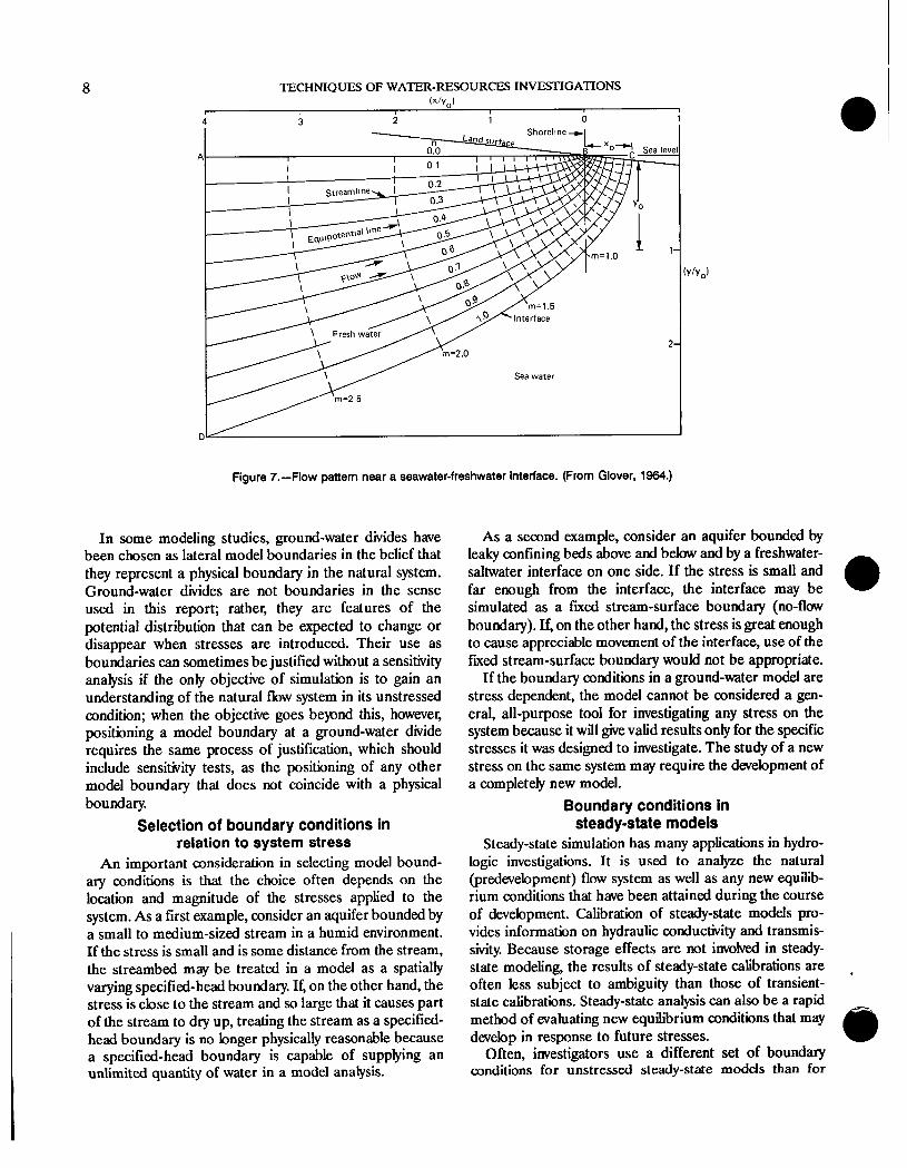
Another example of a free-surface bounda,ry is the transition between freshwater and underlying sea water in a coastal aquifer. If we neglect diffusion and assume the salty ground water seaward of the interface to be static, the freshwater-saltwater transition zone can be treated as a

TECHNIQUES OF WATER-RESOURCES INVESIIGATIONS

Tablel.--Commondesignationsforseveralimportantboundaryconditions

Endary condition name and reference

number in this report

Boundary type and

general name1 Formal Mathematical

name1 Designation

Constant head (1) and

specified head (2)

Type 1 (specified head) Dirichlet h = constant.

Streamline or stream surface (3)

and specified flux (4)

Type 2 (specified flux) Neumann

dh x = constant.

Head-dependent Type 3 dh flux (5) (mixed boundary Cauchy a;r t ch = constant.

condition) (where c is also a constant)

1 See Bear, 1979, p. 96-98

sharp interface and can be taken as the bounding stream surface (no-flow boundary) of the fresh ground-water flm system. It is not difficult to show that, under these conditions, the freshwater head at points on the interface (or within the saltwater body) varies only with the elevation, z (Bennett and Giusti, 1971), and that the freshwater head at any point on this idealized stream-surface boundary is thus a linear function of the elevation of that point, or h= f(z). Line CD in figure 7 is an example of this “idealized” boundary condition, which is both a free- surface and a no-flow boundary.

Because of the inherent difficulty in modeling ground- water systems with free-surface boundaries, the representation of such systems is sometimes facilitated through a set of simplifying assumptions proposed by Dupuit (the “Dupuit assumptions”) in the 19th century. A list and discussion of these assumptions can be found in most textbooks on ground-water hydrology. (See, for example, Freeze and Cherry, 1979, p. 188, 189.)

7. Seepage-sutjkce or seepage-face boundmy (h =z). -A surface of seepage is a boundary between the saturated flow field and the atmosphere along which ground water discharges, either by evaporation or movement “downhill” along the land surface as a thin film in response to the force of gravity. The location of this type of boundary is generally fmed, but its length is dependent on other system boundaries. A seepage surface is always associated with a free surface (boundary condition 6). The junction point (or line in three dimensions) of the seepage face and the free surface (position of junction point determines the length of the seepage face) is generally not known during formulation of a problem but must be determined as a part of the solution. The situation is in that sense analogous to the free-surface boundary, and the equation

expressing the seepage-surface boundary condition is also analogous to that for a free surface: h = z along a seepage face.

Examples of seepage faces are represented by line DE in figure 1A, line BC in figure 5, and line BC in figure 6. Study of the flow nets in these figures shows that the seepage face is neither an equipotential line nor a streamline but a surface of discharge, as mentioned previously. As the illustrations indicate, seepage faces may be associated with individual wells or with earth dams or embank- ments. Seepage faces are often neglected in models of large aquifer systems because their effect is often insig- nificant at a regional scale of problem definition. However, in problems defined over a smaller area, which require more accurate system definition (for example, those depicted in the illustrations cited above), they must often be considered.

Some important aspects of specifying boundary conditions

in ground-water models The preceding sections give a basic introduction to the

boundary conditions most commonly used in modeling ground-water systems. The following discussion provides additional information on boundaries and the specification of boundary conditions in ground-water models.

Model boundaries versus physical boundaries

It is useful to distinguish conceptually between three classes of boundary conditions-those associated with analytical solutions of boundary-value problems, those associated with ground-water-system models (digital for

DEFINITION OF BOUNDARY AND INITIAL CONDITIONS

the most part, but also analog and other types), and those associated with natural (real-world) ground-water systems. The first two classes of boundary conditions are virtually the same except that analytical solutions may involve an unbounded region. Fbr example, in the Theis well solution (see any basic text on ground-water hydrology, for example, Freeze and Cherry, 1979, p. 343), the confined aquifer extends laterally to infinity. Assuming an infinite boundary sometimes simplifies the analytical solution or is necessary in obtaining an analytical solution. Obviously, infinite aquifer dimensions do not occur in natural systems or in numerical, analog, or physical models of them.

In formulating a ground-water modeling problem, it is essential to distinguish carefully between the “physical” boundaries of the natural system and the boundaries of the model. Unfortunately, they are often not the same. To ensure that the proposed model boundaries will have the same effect as the natural system boundaries, the following procedure is recommended: 1. Identify as precisely as possible the natural “physical”

boundaries of the system, even if they are distant from the area of concern;

2. Wherever the proposed model boundaries differ from the natural system boundaries, prepare a careful justification (both conceptually and in the written report of the investigation) to show that the proposed model boundary is appropriate and will not cause the model solution to differ substantially from the response that would occur in the real system.

Simple examples of model boundaries that do not correspond to physical boundaries are lines AI and GH in figure 1A, BF and DG in figure lB, and DE and AF in figure 1C. In all three examples, the natural flow system extends beyond these boundaries, perhaps for a considerable distance. Thus, to model the flow system in the region of interest-that is, close to the engineering structures- it is necessary to establish lateral model boundaries somewhere near the structures. The question of where these boundaries should be located and what conditions should be assigned to them is critical to the success of the model. Experience with many solutions to this general type of problem (two-dimensional seepage flow beneath engineering structures in vertical cross section) indicates that if the distance to the lateral boundaries is at least three times the depth of the flow system, further increases in the distance have only a slight influence on the potential distribution near the structure. In these problems, water flaws from and toward the nearly horizontal constant-head boundaries, and the lateral boundaries are usually designated as bounding streamlines. The many available solutions to problems of this type provide a kind of “sensitivity analysis” on the position of the lateral boundaries. In modeling ground-water systems whose boundaries are more complicated and whose geometries are less regular

7

Figure 6.-Flow pattern in a pemeable dam having vertical faces. (From Wyckoff and Reed, 1996.)

F

Figure 6.-Flow pattern near a discharging well in an unconfined aquifer. (From Nahrgang, 1964.)

than in these examples, a sensitivity analysis may be needed to select an appropriate boundary position and type for a model boundary where no corresponding physical boundary exists. These tests should, of course, be made in the early stages of the investigation.

TECHNIQUES OF WATER-RESOURCES INVESITGATIONS MO)

I I I I I 4 R 2 1 0 1

A 0:o I I I I 01 I I n2

Figure I.-Flow pattern near a seawater-freshwater interface. (From Glover, 1964.)

In some modeling studies, ground-water divides have been chosen as lateral model boundaries in the belief that they represent a physical boundary in the natural system. Ground-water divides are not boundaries in the sense used in this report; rather, they are features of the potential distribution that can be expected to change or disappear when stresses are introduced. Their use as boundaries can sometimes be justified without a sensitivity analysis if the only objective of simulation is to gain an understanding of the natural flow system in its unstressed condition; when the objective goes beyond this, however, positioning a model boundary at a ground-water divide requires the same process of justification, which should include sensitivity tests, as the positioning of any other model boundary that does not coincide with a physical boundary.

Selection of boundary conditions in relation to system stress

An important consideration in selecting model boundary conditions is that the choice often depends on the location and magnitude of the stresses applied to the system. As a first example, consider an aquifer bounded by a small to medium-sized stream in a humid environment. If the stress is small and is some distance from the stream, the streambed may be treated in a model as a spatially varying specified-head boundary. If, on the other hand, the stress is close to the stream and so large that it causes part of the stream to dry up, treating the stream as a specified- head boundary is no longer physically reasonable because a specified-head boundary is capable of supplying an unlimited quantity of water in a model analysis.

As a second example, consider an aquifer bounded by leaky confining beds above and below and by a freshwater- saltwater interface on one side. If the stress is small and far enough from the interface, the interface may be simulated as a fmed stream-surface boundary (no-flow boundary). If, on the other hand, the stress is great enough to cause appreciable movement of the interface, use of the fmed stream-surface boundary would not be appropriate.

If the boundary conditions in a ground-water model are stress dependent, the model cannot be considered a general, all-purpose tool for investigating any stress on the system because it will give valid results only for the specific stresses it was designed to investigate. The study of a new stress on the same system may require the development of a completely new model.

Boundary conditions in steady-state models

Steady-state simulation has many applications in hydrologic investigations. It is used to analyze the natural @development) flow system as well as any new equilibrium conditions that have been attained during the course of development. Calibration of steady-state models provides information on hydraulic conductivity and transmissivity. Because storage effects are not involved in steady- state modeling, the results of steady-state calibrations are often less subject to ambiguity than those of transient- state calibrations. Steady-state analysis can also be a rapid method of evaluating new equilibrium conditions that may develop in response to future stresses.

Often, investigators use a different set of boundary conditions for unstressed steady-state models than for

DEFINlTION OF BOUNDARY AND INITIAL CONDITIONS 9

stressed steady-state or transient-state models of the same system. These “substitute” boundary conditions may offer such advantages as (1) easier interpretation or manipula- tion of model results, (2) ability to model only a part of the flow system, as opposed to the entire system, or (3) easier input to a digital model.

As an example, consider a shallow ground-water system discharging to a small stream. In an unstressed steady- state model of this system, the stream might be treated as a specified-head boundary. Plow to the stream in the model can be calculated from computed heads and compared with field measurements of stream gains. If the model is stressed, howevel; a more complex simulation of the stream may be required, particularly if the stream stage changes in response to the stress. As a second example, the water table is sometimes treated in three- dimensional steady-state models as a specified-head boundary. Inflow to the model through this boundary may be calculated from the model results and compared with field information. Also, treating the water table in this way may permit simulation of only a part of the flow system instead of the entire flow system. In this example the model of the unconfined aquifer behaves as a confined linear system.

In conclusion, these “substitute” boundary conditions usually can be employed only in unstressed steady-state models and, furthermore, they must be compatible with the investigator’s concept of the natural flow system.

The water table as a boundary

Because of the water table’s importance in ground- water systems and, therefore, in system models, the various ways of treating the water table as a boundary that have been discussed are summarized below for reference. 1. The water table is usually conceptualized as a free-

surface recharge boundary-either where recharge equals zero and the water table is a stream surface (as in line CD in fig. 1A, line CD in fig. 5, and line AB in fig. 6) or where recharge equals a specified value (as in fig. 3) and the water table is neither a potential surface nor a stream surface.

2. Sometimes the water table acts as a discharge boundary, particularly where it is near land surface and thus is subject to losses by evaporation and transpi- ration. The discharge from the water table in this case is usually conceptualized as a function of the depth of the water table below land surface-that is, as a function of the water-table altitude. Thus, in a model simulation, the water table is treated as a head-dependent flux boundary. (See the discussion of this boundary condition under “Principal Types of Boundary Conditions.“)

3. As discussed in the preceding section, the water table may also be treated as a specified-head boundary in

unstressed steady-state models; that is, the position of the water table is f=ed as part of the problem definition.

One way in which the water table differs from other boundaries is that it acts as a source or sink of water in transient-state problems because its position is not fixed Because the storage coefficient associated with unconfined, or water-table, storage is large, significant quantities of water are released from storage during a decline in the water table, and, likewise, significant quantities must be supplied for a rise in the water table to occur.

Because the water table is so important in natural systems, and because it has characteristics not common to other system boundaries and may be simulated by boundary conditions that differ significantly from one another in their characteristics, the role of the water table in a specific problem requires special consideration, and its simulation requires particular care.

Reference elevation in ground-water models

In all ground-water models (steady state or transient, absolute head or superposition) a reference elev&n to which all heads in the model relate is required so that the model algorithm can calculate one particular solution to the governing differential equation and associated boundary conditions defining the problem from the existing family of solutions. (See discussion of solution of differential equations in the appendix.) In other words, a reference elevation is needed to define a unique solution to the differential equation governing the problem.

A fLved refemce elevahM is required in steady-state ground-water models. In all types of steady-state models (as well as transient-state models), constant-head or specified-head boundaries (constant-head or specified- head nodes in discretized systems), usually associated with bodies of surface wateg automatically provide a fixed reference elevation. Because most ground-water models have a constant-head boundary somewhere, the question of a reference elevation usually need not be considered explic- itly. Some systems, however, for example a desert valley having internal drainage and a playa on the valley floor, do not have surface-water bodies associated with them. In this example the water table beneath the playa, which is discharging water by evapotranspiration, may be treated as a head-dependent flux boundary, with the rate of discharge from the water table by evapotranspiration defined as a function of the depth of the water table below land surface.

‘As an example of a steady-state problem for which a tied reference elevation is not specified, consider a system that is completely bounded laterally by constant-flux boundaries and has a pumping well within the flow domain whose discharge equals the boundaty flux. Because no reference elevation is specified, this problem has a family of solutions-all with equal gradients but with differing absolute heads-but no unique solution.

10 TECHNIQUES OF WATER-RESOURCES INVESI-IGATIONS

In this example, the reference elevation for the ground- water model becomes the land-surface elevation.

In transient-state models of ground-water systems without constant-head boundaries, the initial heads in the model (the initial conditions) at the beginning of the simulation provide sufficient reference to establish a unique solution to the problem. In a sense, as new sets of head values are calculated for each time step, the reference heads continually change and equal the calculated heads at the end of the preceding time step. In another sense, the heads at the end of any time step are indirectly related to the initial heads in the model.

In summary, a reference elevation is necessary in all types of models to obtain a unique solution to the differential equation governing the problem being simulated. The only case in which the reference elevation in a ground-water-system model requires explicit consideration is a steady-state model without a constant-head boundary.

Concluding remarks The discussions presented herein emphasize the impor-

tance of selecting appropriate boundary conditions for models of ground-water systems. If the boundary conditions used during model calibration are not realistic, the calibration exercise will generally result in erroneous values of transmissivity and storage to represent the system, and predictions made by the model may bear little relation to reality. Even if the transmissivity and storage distributions have been correctly determined, incorrect boundary representation in itself can render the model predictions meaningless.

The selection of boundary conditions is often the most important technical decision made in a modeling project. Alternatives should be considered carefully, sensitivity analysis should always be used, and investigators shoukl always be ready to revise their initial assumptions regard- ing boundaries.

Exercises 1. Choose from a set of cobred pencils a cobr for each

type of boundary condition and trace the fxtent of each boundary type in figures l-7. Upon completion, the cobred lines in each figure should form a continuous, closed curve that outlines each ground- water flow system. Note that the lateral boundaries in figures 1,3, and 4 and the bottom boundary in figure 3 are not physical flcnv-system boundaries and, therefore, will remain uncobred.

2. Make a sketch and designate the boundary conditions of the hypothetical ground-water systems represented by the following well-known formulas:

a. Theis nonequilibrium formula: The assumptions of this formula are listed in many books, careful

consideration should reveal that several of these “assumptions” in fact describe the boundary conditions of the hypothetical ground-water system. How would you set up a numerical model of this problem?

b. Dupuit formula for radial flow under water-table conditions:

Q=W. 2 1

c. Thiem equation for flow to a well in a confined aquifer written in terms of head (h):

Q= 2&m(h,-hi)

In r2/rl -

Consider the various possible relationships between these “model” boundary conditions and the boundary conditions in field situations.

3. Make a sketch in plan view and in cross section of the following types of ground-water systems and designate appropriate boundary conditions. Each system may be represented in several different ways, but most ground-water hydrologists will probably treat some boundary conditions in these systems in the same way

a. An oceanic island in a humid climate; permeable materials are underlain by relatively impermeable bedrock.

b. An alluvial aquifer associated with a medium-sized river in a humid climate; the aquifer is underlain and bounded laterally by bedrock of low hydraulic conductivity.

c. An alluvial aquifer associated with an intermittent

d. A

e. A

stream in an arid climate; the aquifer is underlain and bounded laterally by bedrock of low to inter- mediate hydraulic conductivity. western valley with internal drainage in an arid region; intermittent streams flow from surround- ing mountains toward a valley floor; part of valley floor is playa. confined aquifer bounded above and below by leaky confining beds.

Initial Conditions The results that one obtains from a quantitative model

of a ground-water flow system (head values for various points and times) represent a particular solution to some form of the ground-water flow equation. Ground-water flow equations represent general rules on how ground water flows through saturated earth material. These equations have an infinite number of solutions. An individual ground-water problem must be defined carefully so that the particular solution corresponding to that problem can

DEFINITION OF BOUNDARY AND INITIAL CONDITIONS

be obtained. (See appendix.) Definition of a specific problem always involves specification of boundary-conditions, and in transient-state (time-dependent) problems, the initial conditions must be specified as well.

11

Concept of initial conditions

Definition of initial conditions means specifying the head distribution throughout the system at some particular time. These specified heads can be considered reference heads; calculated changes in head through time will be relative to these given heads, and the time represented by these reference heads becomes the reference time. As a convenience, this reference time is usually specified as zero, and our time frame (expressed in seconds, days, years) is reckoned from this initial time.

In more formal terms, an initial condition gives head as a function of position at t = 0; that is,

h = f(x,y,z; t = 0). (1)

This notation suggests that, conceptually, initial conditions may be regarded as a boundary condition in time.

In formal presentations dealing with the solution of differential equations, boundary conditions and initial conditions are usually discussed together. Problems requiring their specification are known as boundary-value problems and initial-value problems. Analytical solutions are available for a relatively small number of boundary-value and initial-value problems dealing only with simple system geometries (for example, spheres, cylinders, rectangles) and aquifer characteristics that are constant or that vary in a simple way. fir the vast majority of these problems, approximate solution techniques based on numerical methods (simulation) must be used.

The first problem relates to the use of field-measured head values, obtained at a time when the natural ground- water system is at equilibrium, to specify initial conditions in a model. To use these field values of head, the various natural hydrologic inputs (recharge and discharge) and field system parameters (hydraulic conductivity and storage coefficients) that caused the observed distribution of heads must be represented exactly in the model-which is virtually impossible to achieve in practice. Therefore, in a transient-state problem, the initial conditions should be determined through a steady-state simulation of the flow system at equilibrium. After appropriate adjustments of model hydrologic inputs and parameters (process of model calibration), an acceptably close, although not exact, cor- respondence between model heads and field heads is obtained, and the model-generated heads should then be used as initial conditions for subsequent transient-state model investigations. Use of the model-generated head values ensures that the initial head data and the model hydrologic inputs and parameters are consistent. If the field-measured head values were used as initial conditions, the model response in the early time steps would reflect not only the model stress under study but also the adjustment of model head values to offset the lack of correspon- dence between model hydrologic inputs and parameters and the initial head values.

Analytical solutions are often expressed in terms of drawdowns, not absolute heads, and use the principle of superposition. (See Reilly and others, in press). Absolute heads (h = p/r + z) relate to a specific datum of elevation such as in a water-table map, whereas drawdowns are not related to a datum but represent the difference in head between two specific water-level surfaces. If we can use drawdowns rather than absoaCte heads and use the principle of superposidon in solving a specific pmblem, we simplify the task of defining in&l conditions in either ana&tical or modeling problems.

Specifying initial conditions in models

This section discusses two problems in specifying initial conditions in absolute-head models.

The second problem in defining initial conditions is in the simulation of systems that are not in equilibrium, where the objective is to predict the effects of an additional stress on the system at some future time and where absolute heads, rather than superposition, are to be used. In this case the simulation strategy would involve the following steps: (1) identify a period in the past during which the system was in equilibrium’; (2) carry out a steady-state simulation for that period to obtain computed water levels that are acceptably close to measured water levels; (3) use these simulated heads as initial conditions; and (4) model all intervening stresses, including the new stress for which the effects are required, to the specified time in the future.

Of course, if we are interested only in the effect of the additional specified stress on a linear system and are not concerned with predicting absolute heads, we can employ superposition as the simulation strategy (see Reilly and others, in press). The problem of defining initial conditions then disappears because the initial conditions are defined as zero drawdown (or change in head) everywhere in the system.

‘I If a certain pattern of stress on the ground-water system remains unchanged for a sufficiently long period, the system may achieve equilibrium with this stress. Thus, system equilibrium can, but does not necessarily, imply predevelopment conditions.

12 TECHNIQUES OF WA-ER-RESOURCES INVESIIGATIONS ,’ 75

5

z v) z 70 ;I ------

J Eelmated average ground-water level before sewenng

I ul

g P 65 VA t; If z -

;‘ 60

wz

f

\\

3 55

2

2

E Estimated average ground-water level after hydrologx system _ - _ ._

has completely adjusted fo the effects of sewermg ;; 50

:

2 F 245 ’ m ”

1940 1945 1950 1955 1960 1965 1970 1975

Figure 8.--Hydrograph of well N1614 tapping the upper glacial aquifer in central Nassau County, N.Y.

Example of specifying initial conditions in a

field situation Some of the issues concerning the specification of initial

conditions can be discussed in reference to the well hydrograph in figure 8, in which the water level in the well indicates the water-table altitude. The well is in southwest- ern Nassau County on Long Island, N.Y, where a sewer system began operation in the early 1950’s and, by elimi- nating recharge to the water table through septic systems, constituted a stress on the hydrologic system. The sewer system achieved close to maximum discharge by the mid-1960’s. The upper horizontal line (h equals about 69 ft) represents an “merage” water-table altitude at the well (a point) before sewering. The fluctuations in water level around the average value represent a response to the annual cycle of recharge and evapotranspiration and quantitative differences in this cycle from year to year. The lower horizontal line (h equals about 52 ft) represents the average ground-water level after the hydrologic system had completely adjusted to the effects of sewering. By about 1966, the hydrograph seems to “level off’ at this elevation, indicating that the regional sy&em had attained a new equilibrium with the stress of sewering. The water-level fluctuations around the lower horizontal line again reflect only natural recharge and evapotranspiration cycles.

If we were studying a stress in addition to the sewering, and if that stress began in 1975, the lower horizontal line in figure 8 could be taken as the reference level, or initial condition. If we were studying a stress that began in 1963, however, we wuld have to take the upper horizontal tine

as the initial condition and represent the entire sewering operation, as well as the new stress, in the simulation because adjustment of the water levels to sewering would still be in progress in 1963. The decline in head still to occur after 1963 as a result of seweringwould be unknown and could be predicted with confidence only by including the sewering stress in the model study.

Concluding remarks The most important concepts in the application of initial

conditions are as follows: 1. Proper specification of initial conditions in a model of a

natural ground-water system at equilibrium requires initial hydrologic inputs consistent with the initial water levels. To achieve this, it is often necessary to carry out a steady-state simulation of the prepump- ing condition and to use the results as the initial condition for the transient-state simulation.

2. If the natural system is not in equilibrium, a previous period of equilibrium must be identified to specify initial conditions, and all subsequent stresses must be included in the model simulation to predict the absolute head values that will occur at a given future time.

3. Using superposition as part of the modeling strategy simplifies or aMids the need to specify initial coruli- tions. However, superposition modeling predicts only water-level changes related to the specific stress under study and does not predict absolute heads. Furthermore, superposition may be applied only to systems that exhibit a linear (or almost linear) response to stress.


Acknowledgments The authors are deepiy indebted to the other instructors

of the amrse “Ground-Water Concepts,” given at the U.S. Geological Survey’s National Training Center. Over the years, the training materials for this course, including this report, have been generated through a melding of the ideas and work of many individuals, including Eugene Patten, Ren Jen Sun, Edwin Weeks, Herbert Buxton, and others.

References Bear, Jacob, 1979, Hydraulics of groundwater: New York, McGraw-

Hill, 567 p. Bennett, G.D., 1976, Introduction to ground-water hydraulics: U.S.

Geological Survey Techniques of Water-Resources Investigations, Book 3, Chapter B2, 172 p.

Bennett, G.D., and Giusti, E.V., 1971, Coastal ground-water flow near Ponce, Puerto Rico: U.S. Geological Sutvey Professional Paper 750-D, p. D206-D211.

Freeze, R.A., and Cherry, J.A., 1979, Groundwater: Englewood Cliffs, NJ., Prentice-Hall, 604 p.

Glover, R.E., 1964, The pattern of fresh-water flow in a coastal aquifer, in Cooper, H.H., and others, Sea water in coastal aquifers: U.S. Geological Survey Water-Supply Paper 1613-C p. C32C35.

Hubbert, MK, 1940, The theory of ground-water motion: Journal of Geology, v. 48, no. 8, p. 785-944.

Lohman, S.W., and others, 1972, Definitions of selected ground-water terms-Revisions and conceptual refinements: U.S. Geological Sur- vey Water-Supply Paper 1988,21 p.

Nahrgang, Gunther, 1954, Zur Theorie des vollkommenen und unvoll- kommenen Brunnens: Berlin, Springer Verlag, 43 p.

Reilly, T.E., Franke, O.L., and Bennett, G.D., in press, The principle of superposition and its application in ground-water hydraulics: U.S. Geological Survey Techniques of Water-Resources Investigations, Book 3, Chapter B6.

Rushton, RR., and Redshaw, S.C., 1979, Seepage and groundwater flow: New York, John Wiley, 339 p.

Wyckoff, R.D., and Reed, D.W., 1935, Electrical conduction models for the solution of water seepage problems: Physics, v. 6, p. 395-401.

14 TECHNIQUES OF WATER-RESOURCES INVESTIGATIONS

Appendix: Discussion of the Solution of Differential Equations and the Role of

Boundary Conditions

face, sometimes also referred to as the “piezometric surface,” actually traces the static water levels in wells or pipes tapping the aquifer at various points. The differential equation applicable to this problem is obtained by applying Darcy’s law to the flow, Q, across the cross- sectional area, bw, and may be written

The solution of a differential equation describing ground-water flow provides a distribution of hydraulic head over the entire domain of the problem. Fbr simple problems, this distribution of hydraulic head can be expressed formally by a statement giving head as a function of the independent variables. l%r one independent space variable, we may express this statement in general mathematical notation as

h=f(x). (1)

This function, f(x), when substituted into the differential equation, must satisfy the equation-that is, the equation must be a true statement. The function f(x) usually contains arbitrary constants and is called the general solution of the differential equation.

The solution must also satisfy the boundary conditions (and the initial conditions for time-dependent problems) that have been specified for the flow region. To satisfy the boundary conditions, the arbitrary constants in the general solution must be defined, resulting in a more specific function, $(x), which is called the particular solution to the differential equation. Thus, a particular solution of a differential equation is the solution that solves the particular problem under consideration, and the general solution of a differential equation is the set of all solutions. The following example from Bennett (1976, p. 34-44) helps develop these concepts by using the differential form of Darcy’s law as the governing differential equation in a specific problem.

An idealized aquifer system (fig. 9A) consists of a confined aquifer of thickness b, which is cut completely through by a stream. Water seeps from the stream into the aquifer. The stream level is at elevation h, above the head datum, which is an arbitrarily chosen level surface. The direction at right angles to the stream axis is denoted the x direction, and x equals 0 at the edge of the stream. We assume that the system is in steady state, so that no changes occur with time. Along a reach of the stream having length w, the total rate of seepage from the stream (in ft”/s, for example) is denoted 2Q. Because only half of this seepage occurs through the right bank of the stream, the amount entering the part of the aquifer shown in our sketch is Q. This seepage moves away from the stream as a steady flow in the x direction. The resulting distribution of hydraulic head within the aquifer is indicated by the dashed line marked “potentiometric surface.” This sur-

(2)

where K is the hydraulic conductivity of the aquifer and A is the cross-sectional area perpendicular to the direction of flow; in this problem, A is equal to bw.

Integration of the previous equation gives the general solution, f(x), as simply

h=C- Ax,

where C is an arbitrary constant. Two particular solutions from the family of general solutions are shown in figure 9B, one where the arbitrary constant equals zero (eq. a), and one where the arbitrary constant equals h, (eq. b). The differential equation (Darcy’s law) states that if head is plotted with respect to distance, the slope of the plot will be constant-that is, the graph will be a straight line. Both of the lines in figure 9B are solutions to the differential equation. Each is a straight line having a slope equal to

-&. (4)

The intercept of equation a on the h axis is h =0, whereas the intercept of equation b on the h axis is h = h,. These intercepts give the values of h at x = 0 and thus provide the reference points from which changes in h are measured.

The particular solution for the ground-water system depicted in figure 9A is obtained when the boundary conditions are considered. In this problem, the head in the stream, which is represented at x = 0, is designated as the constant h,. Thus, the line in figure 9B that has an h axis intercept of h,, is the particular solution to the problem as posed. Therefore, the particular solution, c(x), of the governing differential equation in this problem is

h=h,- &x.

This solution satisfies the boundary condition at x = 0. An accurate description of boundary conditions in

obtaining a particular solution to any ground-water problem is of critical importance. In multidimensional problems, boundaries are just as important as in the example above, although their effect on the solution may not always be as obvious. Assuming incorrect or inappropriate boundary conditions for a modeling study must inevitably generate an incorrect particular solution to the problem.

DEFINITION OF BOUNDARY AND INlTIAL CONDITIONS 15

Figure Q.-Example of solutions to a differential equation: A, idealized aquifer system; 6, two of the family of curves solving the general differential equation for the idealized aquifer system.

In summary, a particular solution to a differential equation is a function that satisfies the differential equation and its boundary conditions. In numerical models that

simulate the differential equation by a set of simultaneous algebraic equations, the concepts are analogous, although the solution is not a continuous function.

Date post:	17-Mar-2018
Category:	Documents
Upload:	hoangmien
View:	219 times
Download:	1 times