Page 1
| Downloaded From www.singhranendra.com.np |
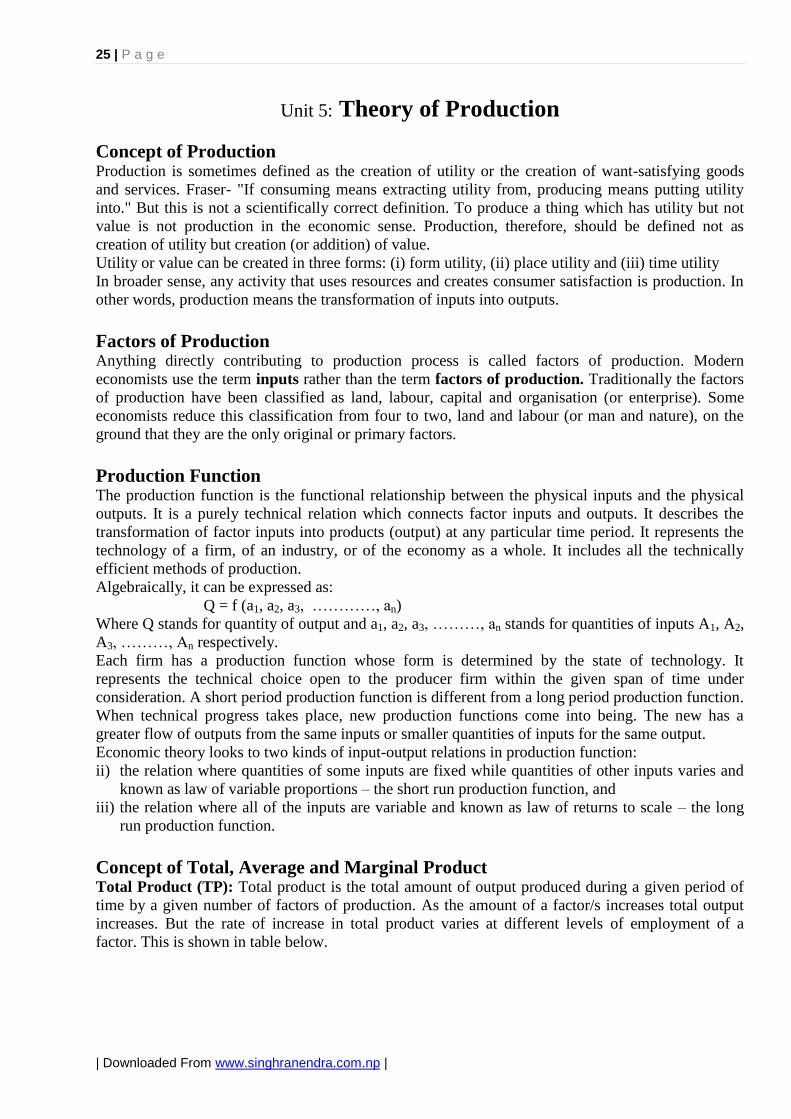
Outp
ut
Class Notes on
Basic economics (For BSc Forestry-first year students)
Prepared by Sanjay K. Upadhyay
Lecturer, IOF Hetauda
2009
Stage I Stage II Stage III
G
F
TP
E
H J
AP
O A B C
MP
Units of Labour
Page 2
1 | P a g e
| Downloaded From www.singhranendra.com.np |
Unit 1: Introduction
Economic Problem: Problem of Scarcity and Choice Concept: Economics is mainly concerned with the utilisation of available material resources to
satisfy human wants. Human wants are unlimited and means to satisfy them are scarce and limited.
The problem of scarcity of resources is felt not only by individuals but also by the society as a whole.
As the resources are limited in comparison to our wants, all our wants cannot be satisfied. Therefore
we have to make a choice between these wants. This gives rise to the problem of how to use scares
resources to get maximum satisfaction. This is generally called the central economic problem, as it
lies at the root of all economic problems faced by the individual and society.
Problem of Scarcity: The economic problem arises from the scarcity of resources relative to
human wants. This gives rise to the struggle of man for existence and efforts by him to promote his
well-being. Every economic system, be it capitalist, socialist or mixed, has to face this problem of
scarcity of resources relative to wants for them. Similarly, every nation, be it developing like Nepal,
India etc. or developed like USA, Germany, France etc. face the problem of scarcity of resources.
However to say that the developed countries, where affluence and prosperity have been brought
about also face this problem raises some doubts. But the fact is that, despite their affluence and
riches, they also face this problem. Because their wants has also increased largely with the increase
in their possession of goods and services. Their present wants still remain ahead of their resources
and capability to produce.
Problem of Choice: Scarcity of resources requires that efficient use of them be made so that the
people get the maximum possible satisfaction. Further, since it is not possible to satisfy all our wants,
due to the scarcity of resources, we face the problem of choice – choice among various wants, which
are to be satisfied. In other words, scarcity of resources in relation to wants gives rise to another
economic problem – the problem of choice, choice among different alternatives. If it is decided to
use more resources in production of one commodity then some resources must be withdrawn from
another commodity. Thus problem of choice from the viewpoint of the society as a whole refers to
which goods and in what quantities are to be produced and productive resources allocated for their
production accordingly so as to achieve greatest possible satisfaction of the people.
The problem of choice is concerned with the following questions:
1) What to produce?
2) How to produce?
3) For whom to produce?
4) What provision should be made for economic growth?
What to Produce: This implies that society has to decide which goods and in what quantities are to
be produced. The society has to choose among hundreds of consumer goods themselves and decide
about allocation of resources between them. Further, it has to decide about what amounts of
consumer goods and capital goods are to be produced. More generally, the society has to choose
among varieties of goods such as clothes, shoes, cars, hospitals, schools, television, rice, oil,
machinery, etc. for production. Moreover, the society must also decide the quantities of the selected
goods to be produced, as it is not possible to produce unlimited amounts of these products.
How to Produce: This means with what combination of resources a society decides to produce
goods. A combination of resources implies a technique of production. Usually various production
techniques are available and the producers have to choose among them. For example a producer may
choose capital intensive or labour intensive techniques for production. Scarcity of resources demands
that goods should be produced with the most efficient method. Therefore it is society's interest that
those techniques of production be used that makes greater use of relatively less scarce resources and
economise relatively more scarce resources.
For Whom to Produce: This means how the national product is to be distributed among the
members of the society. Due to the scarcity of resources wants of all the people cannot be satisfied.
Page 3
2 | P a g e
| Downloaded From www.singhranendra.com.np |
Therefore the society has to decide who should get how much from the total output. In a free market
economy, who would get how much of national output depends on the money income a person
enjoys. Money income can be obtained in the form of wage, rent, interest and profit through utilizing
one‟s labour or property in production process. Differences in the ownership of property and skill in
a free market economy causes differences in money incomes of the people. As a result people with
greater money income enjoy larger share of national output in this economy.
How the national income is to be distributed has been a burning topic not only in the field of
economics but also in politics. Some have argued that all people should get equal incomes and hence
equal shares from the national product. According to Karl Marx, the distribution of national income
should be on the basis of “from each according to his ability to each according to his needs.” Another
important view has been that each individual should get income equal to the contribution he makes to
the national production. In other words, since production is the combined efforts of the factors of
production, i.e. land, labour, capital and enterprise, the national income or output is distributed
among these factors according to their contribution. Landowner gets rent, capitalist gets interest,
labour gets wages and entrepreneur gets profit.
What Provision should be Made for Economic Growth: If all resources available are used for
production of consumer goods only, not leaving any resource for production of capital goods, the
productive resource for production in future will not increase, rather it will decrease due to
depreciation of capital. This means the living standard of the people will decline in the future. This
requires that a part of its resources should be devoted to production of capital goods and to the
promotion of research and development activities. This implies sacrifice of some current
consumption. Therefore a society has to decide how much saving and investment, i.e. how much
sacrifice of current consumption, should be made for future economic progress.
How these Basic Problems are Solved: There are two main methods to solve these basic problems.
One method is to solve these problems through market or price mechanism. That is, all these
problems are decided by the free play of the forces of demand and supply. In such economy, all the
factors of production are basically owned by individuals as private property. Consumers are free to
buy goods according to their desire. Those goods are produced more for which there is greater
demand. Prices of goods as well as factors of production are determined by the forces of demand and
supply. Prices of factors determine the income of the owners of these factors. It is these incomes
which determine the distribution of national outputs among the various individuals in the society.
Similarly, it is prices of the factors according to which the entrepreneurs decide which technique of
production is to be used.
The other method is the adoption of economic planning. In this system, government sets up a central
planning authority which takes decision regarding all these basic problems. In such an economic
system, the capital and property are collectively owned by the society and production is organised by
the government, as well as consumers lose their freedom of choice.
Concept of Microeconomics and Macroeconomics The terms microeconomics and macroeconomics were coined and used by Ragner Frisch in 1933.
The prefixes micro and macro have been derived from Greek words micros, meaning small and
macros, meaning large respectively.
Microeconomics Microeconomics is the study of the economic actions of individuals and small groups of individuals.
It deals with the choice and decision making behaviour of the individual households, firms and
industries and the relationship between prices and quantities of individual goods and services. It
studies economic behaviour of individual economic entities and individual economic variable. In the
words of K. E. Boulding – "Microeconomics is the study of particular firm, household, individual
price, wage, income, industry and particular commodity." Similarly according to Leftwitch –
Page 4
3 | P a g e
| Downloaded From www.singhranendra.com.np |
"Microeconomics concerned with the economic units as consumers, resource owners and business
firms."
Microeconomics studies – (i) how an individual consumer allocate his limited resources to fulfil his
unlimited wants and how he get maximum satisfaction; (ii) how an individual producer allocate his
resources in production process and how he attain equilibrium; (iii) the process of product pricing;
(iv) the process of factor pricing; (v) about efficiency in allocation of resources to consumers and
producers, i.e. welfare theories.
Macroeconomics Macroeconomics is the study of broad aggregates of the economy. It is the study of economic system
as a whole. It studies not one economic unit like a firm or an industry but the whole economic
system. Therefore it deals with totals or aggregate quantities and averages of economy as national
income, total output, total consumption, saving and investment, total employment, general price level
etc. According to Boulding – "Macroeconomics deals not with individual quantities as such but with
aggregates of these quantities, not with individual income but with national income, not with
individual prices but with price levels, not with individual outputs but with national output."
Similarly according to Gardner Ackley – "Macroeconomics concerns itself with such variables as the
aggregate volume of the output of an economy, with the size of national income and with the general
price level." It deals with not only the determination of these aggregates but also how they change
from time to time.
Macroeconomics is concerned with aggregate demand and supply, not with demand and supply of
particular good or individual. It explains how the level of national income and employment is
determined and analyses the factors, which bring changes in these levels. It studies consumption
function and investment function; monetary system of the country, foreign trade, balance of
payments and various subjects relating to public finance. It also deals with national policies as
monetary policy, fiscal policies, foreign exchange policy etc.
Difference between Microeconomics and Macroeconomics 1. Microeconomics is the study of economic actions of individuals and small groups of individuals
as particular households, firms, industries, commodities and prices. Macroeconomics deals with
aggregates of these quantities i.e. national income, general price level, total investment etc.
2. The objective of microeconomics on demand side is to maximize utility and on the supply side is
to maximize profits. Objectives of macroeconomics are full employment, price stability, economic
growth and favourable balance of payments.
3. The subject matter of microeconomics is the price mechanism which operates with the help of
demand and supply forces. These forces help to determine the equilibrium price in the market. The
subject matter of macroeconomics is national income, output and employment, which are determined
by aggregate demand and aggregate supply.
4. Laws of microeconomics are formulated by taking some assumptions. With the help of these
assumptions, microeconomic laws establish relationship between cause and effects of economic
phenomenon. This method of study is known as partial equilibrium analysis. In macroeconomics
economic elements are categorized into aggregate units like aggregate demand, aggregate supply,
total consumption, total investment etc. The interdependence of these economic factors, i.e. the total
effect of an economic factor on the economy is also studied in macroeconomics. This method of
study is known as general equilibrium analysis.
5. Microeconomics states its laws by assuming macro-variables constant. On the basis of these
assumptions, it analyses how production and factors of production are allocated or distributed among
different uses. Macroeconomics assumes micro-variables constant. On the basis of assumption of
constant factor distribution, it explains how full employment can be achieved.
6. Individual demand and supply are the forces of equilibrium in microeconomics. In
macroeconomics aggregate demand and supply are the forces of equilibrium.
Page 5
4 | P a g e
| Downloaded From www.singhranendra.com.np |
Interdependence of Microeconomics and Macroeconomics Though microeconomics and macroeconomics are two different approaches to study and there are
differences between these two approaches, they are not totally independent. Microeconomics
depends on macroeconomics and macroeconomics depends on microeconomics.
Dependence of Microeconomics on Macroeconomics: Change in macroeconomic variables also
influences the microeconomic variables. For instance, when aggregate demand rises during a period
of prosperity, the demand for individual products also rises. If this increase in total demand is due to
the increase in demand of some particular commodities, profits of the firms producing these
commodities also increases. This will increase the demand for the particular types of labours, needed
for these industries. If the supply of such labours is less elastic, its wage rate will rise. Thus a
macroeconomic change also brings changes in the values of microeconomic variables – in the
demand for particular goods, the wage rate of particular industries, the profits of the particular firms
etc.
Dependence of Macroeconomics in Microeconomics: Similarly macroeconomic variables are also
dependent on microeconomic variables. The total is made up of parts. National income is the sum of
the incomes of individual households, firms and industries. Total saving, investment and
consumption are the result of saving, investment and consumption decision of individual firms,
industries, households and persons. The general price level is the average of all prices of goods and
services. For instance, the total level of output, income and employment in the economy also
depends upon income distribution. If income distribution is unequal, i.e., the income is concentrated
in the hands of a few rich people it will reduce the demand for consumer goods. Profits, investment
and output will decline, unemployment will spread and ultimately the economy will face depression.
Thus both microeconomic and macroeconomic approaches to the economic problems are
interdependent.
Page 6
5 | P a g e
| Downloaded From www.singhranendra.com.np |
Market demand curve
0
1
2
3
4
5
6
0 5 10 15 20 Quantity demanded (units)
Pri
ce (
in R
s.)
Rs.
)
Fig. 2.2
Unit 2: Theory of Demand
Demand Function Theory deals with concepts and functions. A function describes the mathematical relationship
between two or more variables. If two variables are related in such a way that for each value of one
of the variables (the independent variable) there corresponds only one value of the other variable (the
dependent variable), then the second variable is said to be a function of the first one.
The demand function for a commodity describes the relationship between the various amounts of the
commodities that might be bought during a given period of time in a given market and the
determinants of those amounts. The determinants are: prices of the commodity, income of the
consumers, their taste and habits, prices of the related goods, etc. Mathematically the demand
function can be expressed as:
Dx = f (Px, Y, Pr, T, u)
Where, Dx is the demand for commodity x, Px is price of the commodity, Y is consumers‟ income, Pr
is prices of related goods, T is measure of consumer‟s taste and habits, u is other determinants of the
demand for x.
Demand Schedules and Demand Curves Demand schedule is a table which shows the quantities of a commodity demanded at different
prices in a given period of time. It states the relation between the two variables of price and quantity.
There are two types of demand schedule- individual demand schedule and market demand schedule.
Individual demand schedule shows the different quantities of a commodity that an individual would
buy at different prices in a certain time period. Market demand schedule shows the different
quantities of commodity demanded at different prices in a market by the whole body of consumers. It
is the total sum of the individual demand schedules in a market. A hypothetical individual and
market demand schedule is shown in the table below considering there are only two consumers in the
market i.e., A and B.
Price
(in Rs.)
Individual demand
(units)
Market
demand
(units) Consumer
A
Consumer
B
1 6 12 18
2 5 10 15
3 4 8 12
4 3 6 9
5 2 4 6
Quantity demanded
0
1
2
3
4
5
6
0 10
Pri
ce
0
1
2
3
4
5
6
0 10 20
Pri
ce
e
0
1
2
3
4
5
6
0 10 20
Pri
ce
e
Quantity demanded Quantity demanded
Demand of consumer A Market Demand Demand of consumer B
d1
D
D
d1 d2
d2
Fig. 2.3
Individual demand curve of consumer A
0
1
2
3
4
5
6
0 2 4 6 8 Quantity demanded
(units)
Pri
ce (
in R
s.)
Fig. 2.1
Page 7
6 | P a g e
| Downloaded From www.singhranendra.com.np |
A demand schedule does not say what the price is. It only says what amounts would be bought at
different possible prices. The lower the price, the larger the quantity that is bought. Similarly, the
higher the price, the smaller the quantity. This inverse relationship between price and quantity
demanded is known as law of demand.
The geometrical representation of demand schedules are called demand curves. Individual and
market demand schedules give individual and market demand curves. When we plot individual and
market demand schedule on a graph we get individual and market demand curves as shown in Fig.
2.1 and Fig. 2.2 respectively. Market demand curve can also be derived graphically by the horizontal
summation of individual demand curves as shown in Fig. 2.3.
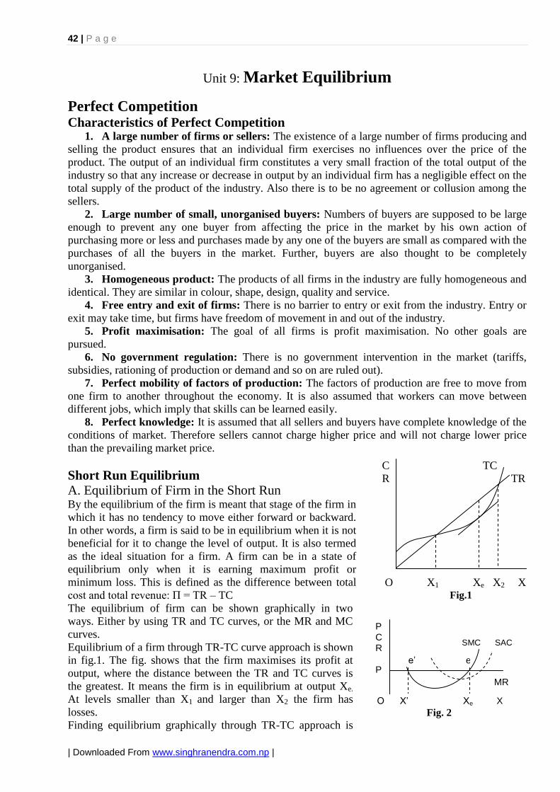
Law of Demand Law of demand states that the demand varies inversely with price, i.e., when the price of a
commodity rises its demand falls and vice-versa, all other things remaining the same. According to
Marshall- "The amount demanded increases with a fall in price and diminishes with a rise in price."
Similarly in the words of Samuelson “ Law of Demand states that people will buy more at lower
prices and buy less at higher prices, other things remaining the same.” For example if quantity
demanded of a product at the price of Rs. 10 is 20 units, more than 20 units will be demanded when
price falls to Rs. 5 and less than 20 units will be demanded when price rises to Rs. 15. This can also
be explained with the help of a diagram (Fig.2.4), where DD is the demand curve. Figure shows that
quantity demanded is D1 at price P1 and rises to D2 when price
falls to P2.
The law does not speak about the effect of demand on price.
Further it only indicates the direction of change but not the degree
of change. It states that the demand varies inversely with price, i.e.
when the price rises demand falls and vice-versa.
Exception to the law 1. Giffen goods: In the mid – 19
th century Sir Robert Giffen
pointed out that in the case of English workers the law of demand
does not apply to bread. He found out that when the price of bread
increased, the low-paid workers in Britain demanded more of it
cutting off demand for meat. This may happen to several other
inferior goods as well called Giffen Goods.
2. Articles of distinction: Distinct commodities like diamonds and jewellery are demanded more
when their price is high. This is because rich people want to show them distinct by having these
goods as ordinary people cannot afford to purchase these goods.
3. Expectation of rise or fall in price in future: If consumers expect that the price of a
commodity rise further in the future they will demand more when price of the commodity rises.
Opposite will happen if they expect further fall in price in future.
4. Ignorance about quality: Sometimes consumers judge the quality of a commodity from its
price. As a result they demand more when price of the good is high assuming the good is of high
quality and vice-versa.
Changes in Demand When demand changes due to the change in price, all other things remaining the same, it is shown on
the same demand curve through two different points as shown in Fig.2.4. In the figure, at price P1
quantity demanded is D1 which rises to D2 when price falls to P2. When demand falls down due to
the rise in price, it is called contraction of demand and when demand goes up due to the fall in
price, it is called extension of demand.
D
P1
P2
D O D1 D2 Quantity
Fig. 2.4
Pri
ce
Page 8
7 | P a g e
| Downloaded From www.singhranendra.com.np |
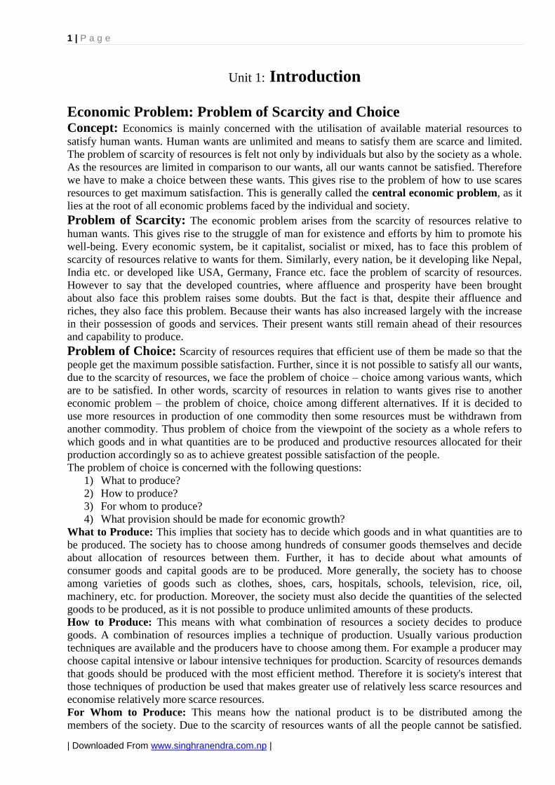
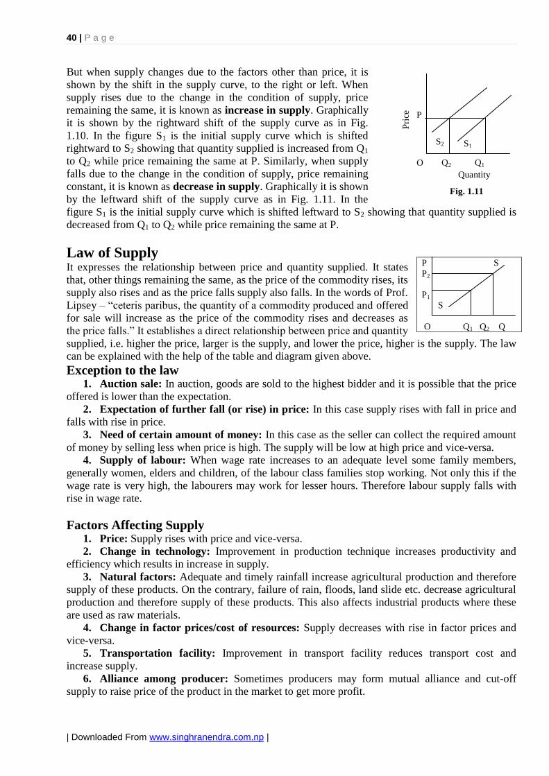
But when demand changes due to the change in factors other than price, it is shown by the shift in
the demand curve, i.e. the movement of the demand curve to the right or left. If demand rises due to
the change in other factors, prices
remaining the same, it is called
increase in demand. Graphically it is
shown by the shift in the demand curve
to the right hand side as shown in
Fig.2.5. Here initial demand curve
D1D1 is shifted to D2D2 showing that
quantity demanded is increased from
Q1 to Q2, price remaining the same at P.
Similarly, if demand falls due to the
change in other factors, prices
remaining the same, it is called
decrease in demand. Graphically it is
shown by the shift in the demand curve to the left hand side as shown in Fig.2.6. Here initial demand
curve D1D1 is shifted to D2D2 showing that quantity demanded is decreased from Q1 to Q2, price
remaining the same at P.
Factors Causing the Change in Demand 1. Price: Demand rises with fall in price of the commodity and vice versa.
2. Change in real income: Demand for a normal good increase with rise in real income and
decrease with fall in real income. But opposite happens in case of inferior goods.
3. Change in prices of related goods: Demand of a good increases when price of its substitutes
rises and vice-versa. But demand of a commodity decreases when price of its compliments rises and
vice-versa.
4. Change in income and wealth distribution: When income and wealth is distributed more
evenly, demand for necessities and comforts increases and that for luxuries decreases. But if income
and wealth distribution is unequal demand for luxuries increases.
5. Change in population: Demand for necessities generally increases with increase in size of
population and vice-versa. Demand also depends on composition of population. For example, if
percentage of old people in total population is increased, demand for walking sticks is increased,
whereas demand for baby foods and diapers is increased in case of increase in percentage population
of children.
6. Change in climate and weather: Demand also changes with change in climate or weather.
For example, demand for ice-cream is increased in summer and demand for woollen clothes is
increased in winter season.
7. Change in tastes, habits, customs and fashion: Changes in people‟s tastes, habits, customs
and fashion also bring changes in demand. For example, as more and more Nepalese people are
being habitual to tea, demand for tea is increasing day-by-day.
8. Effect of advertisement: An attractive advertisement of a product positively influence
consumers which results in increase in demand for the product.
9. Change in the quantity of money in circulation: Purchasing power of people increases
with increase in quantity of money in circulation which results in increase in demand for goods and
services.
10. Technological progress: This brings new things in the market, which replace the old ones.
As a result demand for old things decreases. For example, demand for typewriters is decreased as it
is replaced by computers which are available at low price now-a-days due to the technological
progress.
11. Discovery of cheap substitutes: Discovery of cheap substitute will cause decrease in
demand of a product. For example discovery of nylon decreased demand for silk.
Pri
ce
Fig. 2.5
Quantity
D1
D2
P
D2
Q1
D1
O Q2
Fig. 2.6
Pri
ce
Quantity
D2
D1
P
D1
Q2
D2
O Q1
Page 9
8 | P a g e
| Downloaded From www.singhranendra.com.np |
Unit 3: Elasticity of Demand
Meaning In economics elasticity always has the same meaning. It is the ratio of the relative change in a
dependent variable to the relative change in an independent variable. In other words, elasticity is the
relative change in dependent variable divided by the relative change in the independent variable.
Elasticity of demand is the measure of the degree of change in the amount demanded of the
commodity in response to a given change in its determinant.
Kinds or Elasticity of Demand There are as many kinds of elasticity of demand as its determinants. But the most important of these
elasticities are: (a) the price elasticity of demand, (b) the income elasticity of demand and (c) the
cross elasticity of demand.
Price Elasticity of Demand: It is responsiveness of demand to change in price other things
being unchanged. It measures the extent to which the quantity demanded of a good changes when its
price changes. According to Kenneth Boulding- “elasticity of demand measures the responsiveness
of demand to changes in price.” Similarly, in the words of Marshall- “the elasticity (or
responsiveness) of demand in a market is great or small according as the amount demanded increases
much or little for a given fall in price and diminishes much or little for a given rise in price.”
Marshall was the first economist to give clear formulation of price elasticity as the ratio of a relative
change in quantity to a relative change in price. Let Ep stands for price elasticity, then
Ep =price in change Relative
demand in change Relative
= price in change Percentage
demand in change Percentage
= ΔP/P
ΔQ/Q
Ep is always negative, because of the inverse relationship between demand and price, implied by the
law of demand.
Income Elasticity of Demand: It measures the responsiveness of demand to change in income.
It is the percentage change in amount demanded as a result of a given percentage change in income
of a consumer. In the words of Watson- “Income elasticity of demand means the ratio of the
percentage change in the quantities demanded to the percentage change in income.”
Income elasticity, Ey =income in change Relative
demand in change Relative
= income in change Percentage
demand in change Percentage
= ΔY/Y
ΔQ/Q
For normal goods income elasticity will have a positive sign. For inferior goods income elasticity
will have a negative sign. Sometimes it may be zero in case of several goods.
Cross Elasticity of Demand: It measures the responsiveness of demand for a good to a change
in the price of related good, with own price remaining constant. According to Prof. Ferguson- “The
cross elasticity of demand is the proportional change in the quantity of X demanded resulting from a
given relative change in the price of the relative good Y”.
Page 10
9 | P a g e
| Downloaded From www.singhranendra.com.np |
Cross elasticity, Exy = Yof price in change ateProportion
X of demand in change ateProportion
= yy
xx
/PΔP
/QΔQ
Cross elasticity has a positive sign for substitute goods and a negative sign for complementary goods.
It is zero for independent goods.
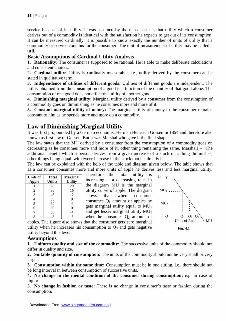
Degrees or Kinds of Price Elasticity of Demand According to the degree of elasticity, price
elasticity of demand can be classified as: (i)
infinitely or perfectly elastic demand, (ii) perfectly
inelastic demand, (iii) relatively elastic demand,
(iv) relatively inelastic demand and (v) unitary
elastic demand.
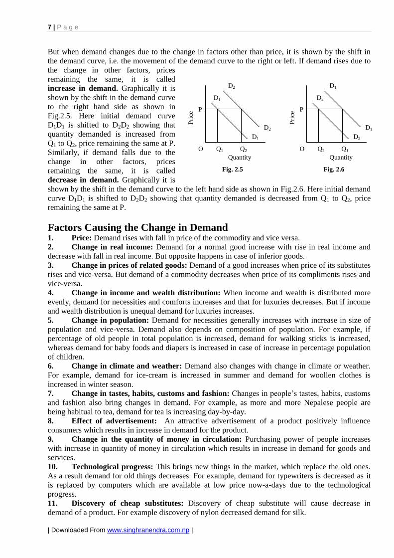
(i) Perfectly elastic demand: When an infinitely
small change in price will cause an infinitely large
change in amount demanded, it is known as
perfectly elastic demand. In this case, a very small rise in price reduce the demand to zero, whereas a
very small reduction in price leads to such a big expansion in demand that no seller is able satisfy
this demand. This means Ep = ∞. This is shown by straight line demand curve parallel to x-axis,
showing demand, as in fig. 3.1. This type of
elasticity hardly exists in real world.
(ii) Perfectly inelastic demand: When demand
remains constant whatever the change in price may
be, it is called perfectly inelastic demand. In this
case Ep = 0. This is shown graphically by a straight
line demand curve parallel to the y-axis, showing
price (fig. 3.2). This type of elasticity also hardly
exists in real world.
(iii) Relatively elastic demand: When a small
relative change in price leads to a considerable change in relative demand, it
is known as relatively elastic demand. In this case 1 < Ep < ∞. This is shown
in fig. 3.3. This type of elasticity occurs mainly in the case of luxurious
commodities.
(iv) Relatively inelastic demand: When a large proportionate change in
price brings only a small proportionate change in demand, it is known as
relatively inelastic demand. In this case 0 < Ep < 1. This is shown in fig. 3.4.
This type of elasticity occurs mainly in the case of necessary commodities.
(v) Unitary elastic demand: When a rise (or fall) in price leads to a fall (or rise) in demand by the
same proportion as price, it is known as unitary elastic demand. In this case Ep = 1. This is shown in
fig. 3.5.This type of elasticity occurs mainly in the case of commodities of comfort.
Determining Factors 1. Availability of substitutes: The demand is elastic for commodities having close substitutes,
e.g. Coke and Pepsi.
2. Nature of the commodity: Demand for necessaries is less elastic or inelastic whereas it is
more elastic for luxuries.
3. Number of uses of a commodity: If a commodity is used for several purposes, the elasticity
of demand is high, e.g. electricity.
4. Possibility of postponing: Elasticity of demand is higher for those commodities whose
consumption or purchase can be postponed.
P d
d
O Q Q
Fig. 3.2
P
d d
P
O Q
Fig. 3.1
P d P d
P1
P2
d P1
P2
d
O Q1 Q2 Q O Q1 Q2 Q
Fig. 3.3 Fig. 3.4
P d
P1
P2
d
O Q1 Q2 Q
Fig. 3.5
Page 11
10 | P a g e
| Downloaded From www.singhranendra.com.np |
5. Level of income: Demand of the commodities consumed by high income group people is less
elastic while that consumed by low income group people is more elastic.
6. Habitual necessities: Those commodities whose consumption is a habit with consumer have
low price elasticity.
7. Proportion of expenditure: Demand for a commodity is less elastic, lesser is the proportion
of expenditure on the commodity by the consumer.
8. Time period: Price elasticity in the short period is low, while in the long period it will be
relatively higher.
9. Prevailing price level: Highly priced commodities and very low priced commodities have
low price elasticity.
10. Jointly demanded goods: In this case elasticity is comparatively low.
Measurement of Price Elasticity of Demand Total Outlay Method Elasticity of demand can be measured from the change in the expenditure of the consumers on the
commodity as its price change. This method was devised by Marshall. He distinguished between
three separate cases of changes in total outlay resulting from a change in the price of the commodity.
1. If with a fall (or rise) in price total outlay increases (or decreases) the elasticity of demand is
greater than one.
2. If with a change in price total expenditure remains constant, elasticity = 1.
3. If with a fall (or rise) in price total expenditure also falls (or rises), elasticity < 1.
The method can be explained with the help of the table given below. Table shows that when price
falls gradually from Rs. 10 to Rs. 6, total expenditure rises from Rs. 10 to reach up to Rs. 30, which
means elasticity is greater than one. Similarly, when price falls from Rs. 6 to Rs. 5, total expenditure
remains constant at Rs. 30, which means elasticity is equal to unity. Finally, when price falls from
Rs. 5 to Rs. 1, total expenditure also falls from Rs. 30 to Rs. 10, which means elasticity is less than 1.
This can also be explained with the help of Fig. 3.6. In the figure curve ABCD shows the total
outlays at different prices of the commodity. Figure shows that from point A to B total outlays rise
with fall in price, which refers EP > 1, from point B to C total outlays remains constant with fall in
price, which refers EP = 1, and from point C to D total expenditure fall with fall in price which refers
EP < 1.
Graphic Method If the changes in price are very small we use as a measure of the responsiveness of demand the point
elasticity of demand. Point elasticity of demand is defined as the ratio of an infinitesimally small
relative change in quantity demanded to an infinitesimally small relative change in price.
Symbolically:
Ep = dQ/Q ÷ dP/P
Price (P)
(Rs.)
Demand (Q)
(units)
Total
expenditure
(P*Q) (Rs.)
EP Direction
of price
Direction of
total
expenditure
10 1 10
>1
=1
<1
9 2 18
8 3 24
7 4 28
6 5 30
5 6 30
4 7 28
3 8 24
2 9 18
1 10 10
Pri
ce
Total expenditure
EP > 1
EP = 1
EP < 1
O
Fig. 3.6
D
B
C
A
Page 12
11 | P a g e
| Downloaded From www.singhranendra.com.np |
or Ep = dQ/dP × P/Q
If the demand curve is linear, Q = b0 – b1P
its slope is dQ/dP = -b1. substituting in the elasticity formula we obtain
Ep = -b1 × P/Q
which implies that elasticity changes at a various points of the
linear demand curve. Graphically the point elasticity of a linear
demand curve is shown by the ratio of the segments of the line to
the right and to the left of the particular point. In fig. 3.7 the
elasticity of the linear demand curve at point F is given by the ratio
FD/FD‟.
Proof:
In fig. 3.7 we have
∆P = P1P2 = EF
∆Q = Q1Q2 = EF‟
P = OP1
Q = OQ1
If we consider very small changes in P and Q, then ∆P ≈ dP and ∆Q ≈ dQ. Thus, substituting in the
formula for the point elasticity, we have
Ep = dQ/dP × P/Q = Q1Q2/P1P2 × OP1/OQ1 = EF‟/EF × OP1/OQ1
Since the triangles FEF‟ and FQ1D‟ are similar, EF‟/EF = Q1D‟/FQ1 = Q1D‟/OP1
Thus Ep = Q1D‟/OP1 × OP1/OQ1 =Q1D‟/OQ1
Furthermore the triangles DP1F and FQ1D‟ are similar, Q1D‟/FD‟ = P1F/FD = OQ1/FD
or Q1D‟/OQ1 = FD‟/FD
Thus the price elasticity at point F is: Ep = FD‟/FD
Given this graphical measurement of point elasticity it is obvious that at
the mid-point of a linear demand curve Ep = 1(point M in fig. 3.7). At any
point to the right of M Ep < 1 and at any point to the left of M, Ep > 1. At
point D, Ep → ∞, while at D‟ Ep = 0.
If the demand curve is non-linear as shown in fig. 3.8, to find out point
elasticity at any point, say M, we draw a tangent to the demand curve at
point M. Then the point elasticity at point M is given by the ratio MB/MA.
Arc Method For measuring price elasticity of demand when the changes in price are somewhat large or the price
elasticity over an arc of the demand curve such as between points A and B in the fig. 3.9 is to be
measured, the concept of arc elasticity has been evolved. In measurement of arc elasticity, we use the
average of original and changed price and average of original and changed demand. Thus the
formula for measuring arc elasticity of demand is:
Ep =
2
q(q
Δq
21 ) ÷
2
p(p
Δp
21 )
=
2
q(q
Δq
21 ) ×
Δp
2
p(p 21 )
= Δp
Δq ×
)
)
21
21
q(q
p(p
The arc elasticity is a measure of the average elasticity, that is, the elasticity at the mid-point of the
chord that connects the two points (A and B) on the demand curve defined by the initial and the new
price levels (fig. 3.9). It should be clear that the measure of the arc elasticity is an approximation of
the true elasticity of the section AB of the demand curve
P D
P1 A
B
P2
D
O Q1 Q2 Q
P D
P1
P2
F
O
E F‟
Q
D‟
Q2 Q1
Fig. 3.7
M
D A
O B
P
Q
D‟
M
P
Fig. 3.8
Fig. 3.9
Page 13
12 | P a g e
| Downloaded From www.singhranendra.com.np |
Unit 4: Theories of Consumers’ Behaviour
The meaning of Utility Every good possesses a quality by virtue of which it satisfies a human want. This want satisfying
power is known in economics as utility. Anything, which satisfies a human want directly or
indirectly, is said to possess utility. Air, water, etc. (free goods) and food, clothes, land, house etc.
(economic goods) satisfy human wants, and as such they possess utility.
Utility is subjective. It varies in from individual to individual. E.g. a pen has no utility for one who
cannot write. Utility varies in different situations. The same thing may possess different utilities for
different purpose. E.g. water has different utilities when used for drinking, bathing or washing. It
also varies with time. A change in taste, season or fashion may affect the utility of a commodity. It is
a relative concept.
Utility may be distinguished from satisfaction. Satisfaction is what we get. It is the result of utility.
If a thing possesses utility, it gives us satisfaction.
Utility and usefulness are not synonyms. If a thing possesses utility it does not necessarily follow
that it is useful. E.g. cigarette is harmful, but it possesses utility for a smoker. The term utility,
therefore as used in economics, has no ethical or moral significance. A thing may be good or bad, but
if it satisfies a human want, we shall say it possesses utility.
Utility is different from pleasure. A good which possesses utility may not give pleasure when
consumed, e.g. medicines. A thing which possesses utility may be tasteful and pleasurable or it may
not give any pleasure.
Forms of utility: (a) form utility – change in utility by changing the form, (b) place utility – change
in utility by changing the place, and (c) time utility – change in utility by storing a good.
Concept of Total, Marginal and Average Utility Total Utility: It is the sum of the utility which he gets by consuming a particular quantity of a
commodity. If a consumer consume one unit, or two, or three, or more at a time he get different
utilities. One unit of commodity yields some amount of utility to the consumer. Two units yield
more, three units still more and so on. As quantities increases total utility increases but total utility
increases at a diminishing rate. To increase total utility at a diminishing rate means that the
successive increments become smaller and smaller. Thus three units have more utility than two, and
four have more than three. Total utility goes increasing till the utility from successive unit reaches to
zero. At this point the consumer is totally satiated. After this level, disutility is obtained and total
utility starts decreasing.
Marginal utility: As we know, when a consumer consumes various units of a commodity, he
obtains higher utility from preceding units and lower utility from succeeding units. The utility
derived from each additional unit is the marginal utility. It may be defined as the addition to the total
utility obtained by the consumption of the last unit. In the words of Prof. Boulding, "Marginal utility
of the quantity of a commodity is the increase in total utility which results from a unit increase in its
consumption." The marginal utility of three units is the addition to the total utility from having three
units instead of two.
MUn = TUn – TUn-1
Average Utility: Total utility divided by the number of units of a commodity consumed gives
average utility. It is the utility obtained from each unit of the commodity consumed in average, that
is the utility per unit of the commodity consumed. As the MU goes on decreasing with increase in
the consumption, AU also tends to fall, but the rate of fall in AU will be lesser than that in MU.
Cardinal Utility Analysis This approach to the theory of demand was started by the classical economists of the late eighteenth
and 19th
centuries but matured at the hands of the 20th
century economists, neo-classicals like
Marshall and Pigou. The basic idea of this approach is that a consumer buys a certain commodity or
Page 14
13 | P a g e
| Downloaded From www.singhranendra.com.np |
service because of its utility. It was assumed by the neo-classicals that utility which a consumer
derives out of a commodity is identical with the satisfaction he expects to get out of its consumption.
It can be measured cardinally, it is possible to know exactly the number of units of utility that a
commodity or service contains for the consumer. The unit of measurement of utility may be called a
util.
Basic Assumptions of Cardinal Utility Analysis 1. Rationality: The consumer is supposed to be rational. He is able to make deliberate calculations
and consistent choices.
2. Cardinal utility: Utility is cardinally measurable, i.e., utility derived by the consumer can be
stated in qualitative term.
3. Independence of utilities of different goods: Utilities of different goods are independent. The
utility obtained from the consumption of a good is a function of the quantity of that good alone. The
consumption of one good does not affect the utility of another good.
4. Diminishing marginal utility: Marginal utility derived by a consumer from the consumption of
a commodity goes on diminishing as he consumes more and more of it.
5. Constant marginal utility of money: The marginal utility of money to the consumer remains
constant to him as he spends more and more on a commodity.
Law of Diminishing Marginal Utility It was first propounded by a German economist Herman Henerich Gossen in 1854 and therefore also
known as first law of Gossen. But it was Marshal who gave it the final shape.
The law states that the MU derived by a consumer from the consumption of a commodity goes on
decreasing as he consumes more and more of it, other thing remaining the same. Marshall – "The
additional benefit which a person derives from a given increase of a stock of a thing diminishes,
other things being equal, with every increase in the stock that he already has."
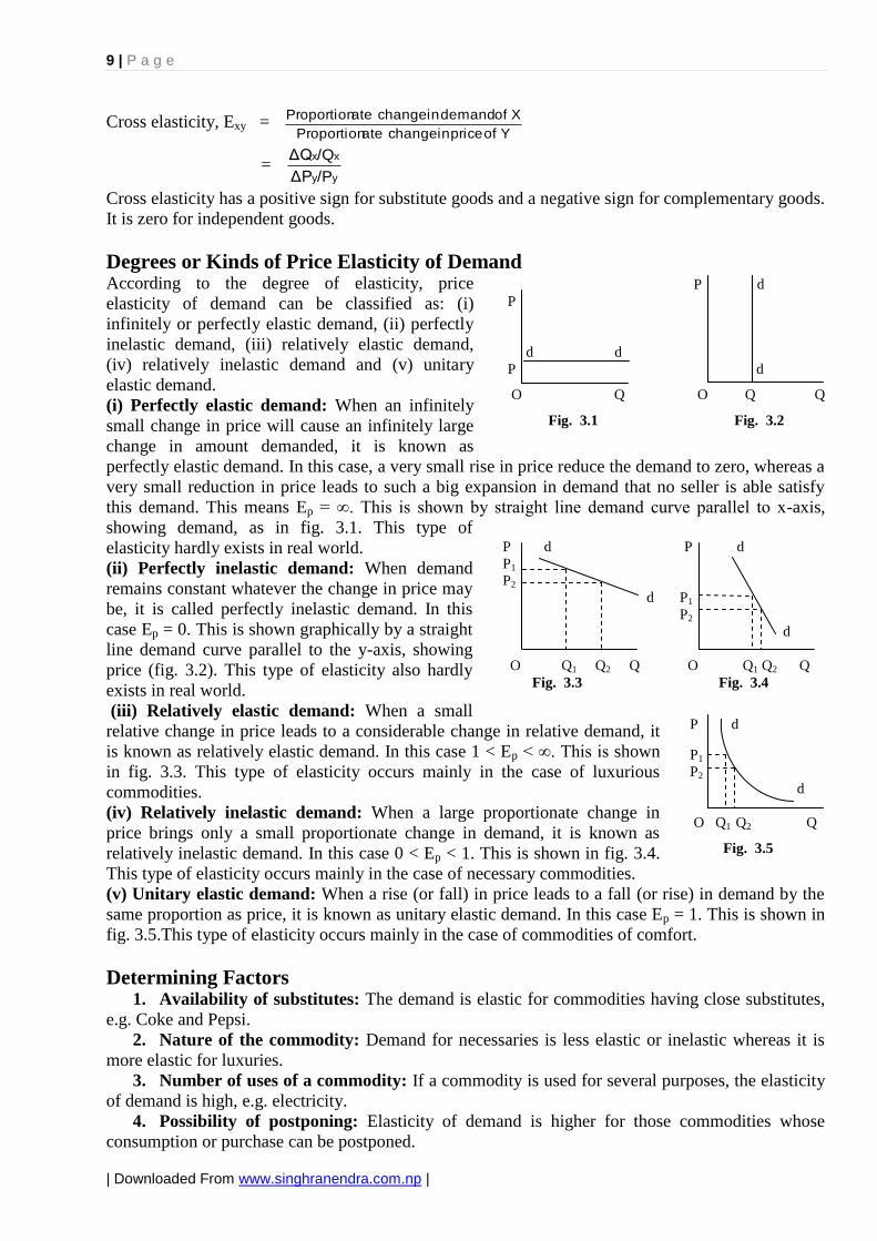
The law can be explained with the help of the table and diagram given below. The table shows that
as a consumer consumes more and more units of apple he derives less and less marginal utility.
Therefore the total utility is
increasing at a decreasing rate. In
the diagram MU is the marginal
utility curve of apple. The diagram
shows that when consumer
consumes Q1 amount of apples he
gets marginal utility equal to MU1
and get lesser marginal utility MU2
when he consumes Q2 amount of
apples. The figure also shows that the consumer gets zero marginal
utility when he increases his consumption to Q3 and gets negative
utility beyond this level.
Assumptions 1. Uniform quality and size of the commodity: The successive units of the commodity should not
differ in quality and size.
2. Suitable quantity of consumption: The units of the commodity should not be very small or very
large.
3. Consumption within the same time: Consumption must be in one sitting, i.e., there should not
be long interval in between consumption of successive units.
4. No change in the mental condition of the consumer during consumption: e.g. in case of
liquor.
5. No change in fashion or taste: There is no change in consumer‟s taste or fashion during the
consumption.
Units of
Apple
Total
Utility
Marginal
Utility
1
2
3
4
5
6
7
8
20
36
48
56
60
60
56
48
20
16
12
8
4
0
-4
-8
Utility
MU1
MU2
O Q1 Q2 Q3
Units of Apple MU
Fig. 4.1
Page 15
14 | P a g e
| Downloaded From www.singhranendra.com.np |
6. No change in the price of the commodity or its substitute: It is assumed that the commodity's
price is not changed with successive units and the price of the substitute also remains the same.
Exceptions or Limitations 1. Rare and curious goods: Law does not apply to rare and curious goods like old coins, rare
paintings etc.
2. Goods of display: Things, which satisfy consumers' taste for display of his wealth or fashion
such as jewellery.
3. Consumption of public goods: The law does not apply to such public goods as telephones
because the greater the number of telephones in a town, the greater is the utility obtained from the
use of a telephone.
4. Intoxicants: as intoxicants change the mental condition of the consumer as they consume more
and more of it.
5. Poetry, music or good books: These may give interested persons more and more utility.
6. First time consumption of a commodity: In this case he may get increasing marginal utility for
some time.
Theoretical and Practical Importance 1. Basis of some economic laws: Several very important laws and concepts of economics are based
on this law e.g., law of demand, the concept of consumer's surplus, the concept of elasticity of
demand, law of substitution.
2. Importance to finance minister: A finance minister takes this law as guideline for taxation. He
taxes the commodities purchased by the rich at a high rate and those purchased by poor people at a
low rate. Similarly, in case of income tax, the rich are taxed at higher rate, because MU of money to
them is lower than that to the poor. This is called progressive taxation.
3. Importance to the consumer: This law also works as a guideline to the consumer. He is advised
to spend his income over the purchase of a number of commodities rather than on one commodity
due to which he can get the maximum utility out of his expenditure.
4. Value in use and value in exchange: The law help us to know the difference between value in
use and value in exchange. Water has high value in use but no value in exchange because the MU of
another unit of water is zero. On the other hand the value in exchange of a commodity like gold is
very high because its MU is quite high.
5. Socialism: Socialists take their stand on this law when they advocate a more equal distribution of
wealth. They suggest to transfer some part of wealth with the rich to the poor through taxation and
grants. They argue that the measure of sacrifice by the rich in terms of utility is much less as
compared to the utility obtained by the poor. There is a net gain to society through this income
transfer.
Does This Law Apply to Money? It seems that the law of diminishing MU does not apply to money. Money is a general purchasing
power. It enables the purchaser to buy anything he likes. Hence it is said that no person ever feels
satisfied with money, however rich he may be. But slightly deeper thinking clearly tells us that this is
not so. The MU of money also diminishes with the increase in money a man has. The importance of
money to a rich man is not so much as it is for a poor man. A rich man spends it more freely and is
much less worried in case he happens to lose a certain portion of it. Every increment in the amount of
money that a man has brings him less and less extra pleasure. Hence the law of DMU applies to
money also. There is no doubt that the utility of money diminishes slowly and is perhaps never zero.
This is because money can buy any other commodity or service.
Law of Substitution This law was also propounded by Gossen and therefore also known as second law of Gossen. But the
final shape was given by Marshall. This law is also called law of maximum satisfaction or law of
equi-marginal utility or law of indifference.
Page 16
15 | P a g e
| Downloaded From www.singhranendra.com.np |
The law states that to get maximum utility from the expenditure of his limited income (budget), the
consumer purchases such amount of each commodity that the last unit of money spent on each of
them gives him the same MU. The consumer is faced with a choice among many commodities that
he can and would like to buy, and his income is always insufficient to buy all the commodities for
him and as much as he likes. Therefore, he would get maximum utility or satisfaction only if he
allocates his limited income on the purchase of different commodities in such a way as yields him
the same MU in all. For this the consumer substitutes some units of the commodity of greater utility
for some units of the commodity of less utility. As a result the MU of the former will fall and that of
the latter will rise, till the two MUs are equalised. This can be explained more clearly with the help
of a numerical example. Suppose, a consumer has Rs. 6, which he wants to spend on apples and
oranges, so that he obtains the maximum total utility. The following table shows the MU of spending
successive rupees of income on apples and oranges. From the table we can easily see that the
consumer obtains maximum total utility equal to 98 utils by spending Rs.
4 on apples and Rs. 2 on oranges, i.e. when MUs of both are equal to 14
units. Any other allocation of his budget will give him less total utility.
The law can also be explained with the help of a diagram (fig. 4.2). In
the figure curve MUa represents marginal utility of apple and curve MUb
represents marginal utility of banana of spending one unit of money and
MUm represents the marginal utility of money. The diagram shows that
the consumer, with total money equal to OM+ON, will gain maximum
satisfaction if he spends OM units of money on bananas and ON
units on apples, i.e. when marginal utility of spending last unit of
money on both the commodities are equal (OR in the figure). Any
other combination will give him lesser satisfaction. For example if
the consumer decides to spend OM‟ on banana and ON‟ on apples
(here MM‟=NN‟) rather than the former combination, his utility
from banana will increase by area MABM‟ whereas his utility from
apple will decrease by area N‟CDN, which is larger than the area
MABM‟. This means this combination will give him lesser total
utility than the former combination.
We have shown here in the table and in the diagram only two
commodities. Actually, the consumer purchases many commodities at the same time. But the same
principle applies to all of them i.e., the MU of expenditure of the last (marginal) unit of money on all
of them must be the same. MU of expenditure on a commodity is defined as the ratio of MU to its
price. Therefore, the condition for maximisation of utility is given by:
MUa/Pa = MUb/Pb = MUc/Pc = …………… = MUn/Pn
Assumptions 1. Consumer is rational.
2. The utility is cardinally measurable.
3. MUs of the different commodities are independent of each other.
4. MU diminishes with more and more purchases.
5. The consumer has a limited amount of income to spend.
6. MU of money remains constant.
Criticism or Limitations 1. Effect of fashion and customs: Human being spend a lot of their money income on fulfilling
social customs and fashions such as marriage ceremonies, birth day parties, death ceremonies etc.
these acts are not done in the basis of the law of substitution. People even sacrifice higher utility, if
custom and fashion is so required.
2. Individual goods: The law does not apply in the use of indivisible goods. The reason is that the
consumer cannot divide the goods to adjust the units of utilities derived from their consumption.
Units
of
money
MU of
apple
(Utils)
MU of
banana
(Utils)
1
2
3
4
5
6
20
18
16
14
12
10
16
14
12
10
8
6
Fig. 4.2
Uti
lity
Units of money
R
N‟ N M M‟ O
MUm
MUa MUb
A
B
C D
Page 17
16 | P a g e
| Downloaded From www.singhranendra.com.np |
3. Utility cannot be measured: The law is based on the assumption that utility is cardinally
measurable. But in reality it is not possible. Utility is subjective and can only be felt. We cannot
measure it in exact number.
4. Non availability of goods: The law does not apply when the goods of choice of consumers are
not available in the market. In such a case, the consumer will have to buy a good which gives him
lesser utility.
5. Lethargy of the consumer: Calculation of utility is very tiresome and therefore many
consumers do not bother to calculate it. Thus they do not act according to the law.
6. Unlimited supply: The law does not apply to goods of unlimited supply like as free gift of
nature.
Importance 1. Production: In production process various factors of production are used by the producer. To get
maximum profit, he substitutes one factor for another to the point where marginal returns from all
the factors are equal.
2. Consumption: In allocation of his income between consumption and saving the consumer tends
to equate the marginal gain from an increase in consumption to the marginal loss from the resultant
decline in saving. Similarly in spending his income on different commodities he tends to equate the
marginal utility from the marginal units of money expenditure on each commodity.
3. Exchange: Exchange means substitution of one thing for another. The consumer exchange one
commodity with other in such a way that the MU from both the commodities is equal.
4. Distribution: The share of each factor of production is determined on the basis of the principle
of marginal productivity. The various factors are used in such a manner that the marginal product of
each factor is equal.
5. Public finance: The law also works as the guideline for the government in public expenditure.
The public revenues are so spent as to secure maximum welfare for the society. For this the
government cut down expenditure where the return is low and increase expenditure on more
productive or more beneficial works.
6. Allocation of time: The law also guides an individual in the allocation of his time between work
and leisure. He must equate the MU of income from an hour's more work to the MU of leisure,
which he has to forgo.
Derivation of Demand Curve Derivation of demand curve is shown in the figure here.
Figure shows the consumer's MU curves for expenditure
on commodity X at two different prices. It is assumed that
the MU of money (MUm) is constant equal to OH. For
equilibrium of the consumer, the MU/P ratio must equal to
MUm. At price P1, consumer purchase OM1 amount
because at this level MUx/P = MUm. This gives point d1.
At price P2 consumer will purchase OM2 amount. This will
give point d2 and so on. Joining d1, d2 and so on we get the
demand curve as shown in the figure.
Criticism
1) Utility is subjective while demand is objective
phenomena.
2) Difficult to measure utility.
3) Utilities of commodities are not independent.
4) It assumes too much and proves too little.
5) Unrealistic assumption of constant MU of money.
6) Only a particular equilibrium theory. It becomes inconsistent when we apply it to the case of two
commodities.
MU/P MUx/P1 MUx/P2
H MUm
O M1 M2
Quantity of X
P1 d1
P2 d2
O M1 M2
Quantity of X
Pri
ce
Fig. 4.3
Page 18
17 | P a g e
| Downloaded From www.singhranendra.com.np |
7) Ignores income effect.
8) Fails to explain Giffen Paradox.
Consumer’s Surplus Sometimes a consumer feels that he is deriving more satisfaction from the consumption of a
commodity than the amount of sacrifice he makes in money terms while getting it. This feeling in
consumer's mind has been given the name of consumer’s surplus. It is the difference between what
we are prepared to pay and what we actually pay. The concept of consumer‟s surplus was invented
by A.J. Dupuit. But the concept was fully developed and was brought into use by Marshall. Marshall
defined consumer‟s surplus as "the excess of the price which a person would be willing to pay rather
than go without the thing over that which he actually does pay." We can put it in the form of an
equation thus:
Consumer's surplus = Total utility – Total amount spent
This can be explained with the help of a table given below. In the table marginal utility is expressed
in terms of money (Rs.). Table shows that the total consumer‟s surplus is equal to Rs. 40 (=60-20).
The concept can also be explained graphically with
the help of Fig. 3.3. In the figure, DD is the demand
curve of a product which also shows the amount of
money a consumer wants to pay for various amount of
the commodity, i.e. the marginal utility of the
consumer in monetary term. Now if the price of the
product is OP, consumer will purchase OQ amount of
the product. His total expenditure will be equal to area
OPMQ and total utility will be equal to area ODMQ.
This means his surplus will be equal to area DPM.
Assumptions 1. Utility can be measured cardinally.
2. MU of money remains constant.
3. No change in income, taste and fashion.
4. No substitute is available.
5. MUs of different commodities are independent of each
other.
Criticism 1. Imaginary: It is purely imaginary concept. It is not found in
real life. No one will be willing to pay more than the price of the commodity. Actual price and
willing price are always equal in real life.
2. Difficult to measure: It is difficult to measure exactly. It is a subjective concept and majority of
consumers cannot express it in quantitative term.
3. Not applicable to essential necessaries: For these commodities the consumer will be prepared
to pay any price and therefore the consumer's surplus will be infinite in this case.
4. Unrealistic assumptions: Assumptions of cardinal measurability, constant marginal utility of
money etc. are unrealistic.
5. Not found in practice: In practice a consumer will switch over to other commodity whose MU
is higher before he reaches the point of marginal utility – price equality.
Importance 1. In public finance: Concept is useful to finance minister in imposing taxes and fixing their rates.
He fixes higher rate of tax on those commodities which gives the consumers higher surplus. This
will bring more revenue to the government while the consumers have to sacrifice comparatively
less utility.
Units of
Apple
Marginal
Utility
Price (Rs.) Consumer’s
surplus
1
2
3
4
5
20
16
12
8
4
4
4
4
4
4
16
12
8
4
0
Total
units = 5
Total
utility =
60
Total
amount
spent = 20
Total = 40
P
Q O
M
D
D
Pri
ce
Quantity
Fig. 4.4
Page 19
18 | P a g e
| Downloaded From www.singhranendra.com.np |
2. To the businessman and monopolist: The businessman can raise prices of those commodities in
which consumer's surplus is high and get more profit. Further, if the seller is monopolist, he can
control supply and charge high price.
3. Comparison of levels of living in different places: The concept helps in comparing the
standards of living between two places where money income is the same but other factors differ.
In those places where there are greater amenities of life and civic facilities available at low price,
people will enjoy large consumer's surplus and better living.
4. Difference between value-in-use and value-in-exchange: The concept helps to distinguish
between value in use and value in exchange. For ex. We have much consumer's surplus from
news papers, matchsticks, postcards etc. as we have to pay a very low price for them while they
have high utility. In other words, value-in-use in case of such commodities is much higher than
their value-in-exchange. The consumer's surplus depends on total utility whereas price depends
on marginal utility.
5. Measuring benefits from international trade: The concept is helpful in explaining the
advantages of international trade. It is said that a country must so arrange its imports and exports
that the consumer's surplus in the country maximised. Likewise the government can tax relatively
cheap imports to extract part of the consumer's surplus.
6. In the pricing of public utilities: It is advised that the government should discriminate between
various users of public utility services according to the measure of consumer's surplus they got
from it and should fix different charges according to the principle of price discrimination.
Ordinal Utility Analysis: The Indifference Curve Theory Concept of Indifference Curve
English economist F.Y. Edgeworth invented it in late 19th
century. Italian economist Vilfredo Pareto
put it to extensive use.
Russian economist Slutsky was the first to explain the law of demand using indifference curve
approach in 1915. Detailed study of indifference curve approach to the law of demand was given by
English economists Hicks and Allen in 1928 in a paper ' A Reconsideration of the Theory of Value',
Economica, 1934. Later Hicks wrote the theory in more detail in his book 'Value and Capital',
published in 1939.
Assumptions 1. Rational behaviour of the consumer: He aims at the maximisation of his utility or satisfaction
given his income and market prices.
2. Utility is ordinal: It cannot be measured but put into an order.
3. Scale of preference: Consumer is able to arrange the available combinations of goods according
to preference or indifference for them.
4. Diminishing marginal rate of substitution: As the amount of a commodity with the consumer
increases, he will be ready to exchange lesser and lesser amount of the other commodity for equal
unit of the commodity whose amount is increasing.
5. The total utility of the consumer depends on the quantities of the commodities consumed: U
= f(q1, q2, ………, qn).
6. Consistency and transitivity of choice: If the consumer chooses bundle A over B in one period,
he will not choose B over A in another period, if both bundles are available to him. Similarly if
bundle A is preferred to B and B is preferred to C, then bundle A is preferred to C.
7. Scale of preference is independent of the market prices. 8. Assumption of continuity: Consumer can rank all conceivable combinations of goods according
to his preference and indifference.
Indifference Schedule and Curve
An indifference schedule is a list of the various combinations of goods which give equal satisfaction
to the consumer. Table given below contains a hypothetical indifference schedule taking two
commodities orange and apple.
Page 20
19 | P a g e
| Downloaded From www.singhranendra.com.np |
We can convert the indifference schedule into an indifference curve
by plotting these combinations on a graph paper. An indifference
curve is the locus of points, particular combinations or bundles of
goods, which yield the same utility (level of satisfaction) to the
consumer, so that he is indifferent as to the particular combinations
he consumed. Symbolically it is given by the equation:
U = f(x1, x2, ………, xn) = k.
An indifference curve is generally presented graphically by taking
two commodities at a time, i.e. one on the x-axis and the
other on y-axis, as shown in fig.4.5.
Indifference Map An indifference map shows all the indifference curves
which rank the preferences of the consumer.
Combinations of goods situated on an indifference
curve yield the same utility. Combinations of goods
lying on a higher IC give higher satisfaction and are
preferred. Combinations of goods lying on a lower IC
give lower utility. An indifference map is shown in
fig.4.5.
The Marginal Rate of Substitution (MRS) The marginal rate of substitution of x for y is defined as the number of unit of commodity y that must
be given up in exchange for an extra unit of commodity x so that
the consumer maintains the same level of satisfaction.
The MRS between two commodities is shown by the shape of the
IC showing their combinations. Mathematically it is written as:
MRSx,y = ∆y/∆x
(and more accurately, MRSx,y = -dy/dx = slope of the IC)
The convex indifference curve falling from left down to the right
shows the law of diminishing MRS. Hicks has given his
justification for assuming a diminishing MRS. There are two
reasons for this: (i) each particular want is satiable. Therefore as
a consumer obtains more and more of one commodity his
intensity of the need for it goes on diminishing. As a result, the
consumer will be prepared to sacrifice less amount of the other
commodity in order to get more and more of this commodity.
(ii)Goods are imperfect substitutes for one another.
Properties of Indifference Curves 1. Higher ICs represent higher level of satisfaction: In fig. 4.7
combination B (x2, y2) includes more of commodities X and Y and
therefore gives more satisfaction than combination A (x1, y1). This
means IC2 gives more satisfaction than IC1.
2. ICs slope from left downward to the right: It cannot be parallel
to x-axis as shown in fig. 4.8. Because in this case combination B (x2,
y1) gives more satisfaction than combination A (x1, y1). Similarly, it
cannot be parallel to y-axis as shown in fig. 4.9, as in this case
combination B (x1, y2) gives more satisfaction than combination A
(x1, y1). It cannot be upward sloping as shown in fig. 4.10, as in this case combination B (x2, y2)
Combination Orange Apple
A 1 15
B 2 11
C 3 8
D 4 6
E 5 5
Y
Δy
IC
O X
Y
y2 B
A
y1
IC2
IC1
O x1 x2 X
Fig. 4.7
Co
mm
od
ity
Y
Commodity X
IC2
IC1
IC3
O
Fig. 4.5
Δx
Fig. 4.6
Page 21
20 | P a g e
| Downloaded From www.singhranendra.com.np |
gives more satisfaction than combination A (x1, y1). Therefore the only possibility is that it slopes
from left downward to the right.
3. The ICs are convex to the
origin: It cannot be straight line as
shown in fig.4.11. Because in this
case marginal rate of substitution
(Δy/Δx) is constant throughout the
curve, which is violation of the
axiom of diminishing marginal rate
of substitution. Similarly it cannot
be concave to the origin as shown in fig. 4.12. Because in this case MRS is increasing from left to
right, which is violation of the axiom of diminishing MRS. Therefore it can only be convex to the
origin as shown in fig. 4.13.
4. ICs do not intersect each
other: If they intersect each
other as shown in fig. 4.14 then
the point of intersection shows
two different level of satisfaction
which is impossible. In fig. 4.14
point A gives higher level of
satisfaction than point B as the
former combines more of
commodities X and Y. The point
of intersection C lies both on IC1 and IC2
which implies C = A as well as C = B, which
is impossible.
5. ICs may not be parallel
6. ICs do not touch the axes: If it touches
the axes as shown in fig.4.15 then it implies
that there is perfect substitutability between
commodity X and Y which is violation of
the assumption of imperfect substitutability.
7. ICs for perfect substitute and perfect
components: If commodities are perfect substitutes the IC becomes a straight line with negative
slope as shown in fig. 4.16. If the commodities are complements the IC takes the shape of a right
angle (fig. 4.17). In the first case the equilibrium of
the consumer may be a corner solution, that is, a
situation in which the consumer spends all his income
on one commodity. These situations are not observed
in the real world and are usually ruled out from the
analysis of the consumer‟s behaviour. In the case of
complementary goods, IC analysis breaks down, since
there is no possibility of substitution between the
commodities.
The Budget Constraint
In order to study consumer‟s behaviour, we assume that the consumer has the given income with
which he wants to purchase at the given prices of the commodities. Income acts as a constraint in the
attempt for maximising utility. The consumer wants to go higher and higher up on his ICs in his
indifference map. But choice is limited to the combinations of the commodities he can purchase with
Y
y1 A B
IC
O x1 x2 X
Fig. 4.8
Y IC Y IC
y2 B y2 B
y1 A y1 A
O x1 X O x1 x2 X
Fig. 4.9 Fig. 4.10
Y
Y Y
Δy Δy Δx Δy Δy Δx Δx Δy Δy Δx Δx Δx Δy Δx O X O X O X
Fig. 4.11 Fig. 4.12 Fig. 4.13
Y Y
C
A IC1
B IC
IC2
O X O X
Fig. 4.14 Fig. 4.15
Y Y
O X O X
Fig. 4.16 Fig. 4.17
Page 22
21 | P a g e
| Downloaded From www.singhranendra.com.np |
his given income at the given prices. The income constraint in the case of two commodities, may be
written as:
Y = pxqx + pyqy.
We can present the income constraint graphically by the budget line,
whose equation is derived from the above expression, by solving for qy:
qy = (1/py) Y – (px/py) qx
Assigning successive values to qx (given the income Y and the
commodity prices px, py) we may find the corresponding values of qy.
Thus, if qx = 0, i.e. if the consumer spends all his income on y, the
consumer can buy Y/py units of y. Similarly if qy = 0, qx = Y/px. In the
figure, these results are shown by the points A and B. If we join these
points with a line we get the budget line. Slope of this line is
OA = Y/py = px
OB Y/px py
Mathematically the slope of the budget line is the derivative
δqx/δqy = px/py
The budget line or price line shows all those combinations which can be bought by the consumer at
the given prices. It shows the possible combinations of consumer‟s consumption.
If consumer's income or the price of the commodities changes the price line also changes its position.
This is shown in fig. 4.19 and 4.20.
1. Change in consumer’s income: If
prices of the commodities remain constant, the
price line shifts parallel to the right with
increase in the consumer‟s income and to the
left with decrease in his income.
2. Change in price of the commodity: If
income being the same, change in price of any
one of the commodities results in a change in
the slope of the price line.
Equilibrium of the Consumer Given the indifference map of the consumer and his price line,
we can find out the combination, which gives him maximum
satisfaction. For this we superimpose the price line on
consumer's indifference map as in fig. 4.21. The aim of the
consumer is to get maximum satisfaction. So he tries to go to
the highest indifference curve attainable with his given price
line. The consumer will be in equilibrium at that point
(combination of goods) which lies on his price line as well as at
the highest possible IC. This condition is fulfilled at point E in
the fig. Therefore the consumer will be in equilibrium at point
E, i.e. he will get maximum satisfaction by consuming
xe and ye amounts of the commodities X and Y. It is also clear
from the figure that the equilibrium point of the consumer is the point of tangency of the budget line
with the highest possible IC. At the point of tangency the slope of the budget line (px/py) and the IC
(MRSx,y) are equal.
MRSx,y = px/py
This is the first order condition (being tangent to IC) for equilibrium. The second order condition is
implied by the convex shape of the IC, i.e. diminishing MRS.
y
Y/py
A
Y/px
O B x
Fig. 4. 18
Y Y
L2 L
L1
O M1 M2 X O M1 M2 X
Change in income Change in price
Fig. 4.19 Fig. 4.20
Y
L
ye E
IC3
IC2
IC1
O xe M X
Fig. 4.21
Page 23
22 | P a g e
| Downloaded From www.singhranendra.com.np |
Income Effect With a change in consumer‟s income, prices of the
commodities being the same, his budget line shifts parallel to
the right if income increases and to the left if it decreases as
shown in the figure. As a result the equilibrium points also
changes. Joining all these equilibrium points (E1, E2, E3 in
fig. 4.22) we get a curve called income consumption curve
(ICC). The amount of change in demand due to change in
income is called income effect. In the figure x1x2 and y1y2 is
income effect.
The ICC can take different shapes according to the type of
the commodity. If both the
commodities are normal, the income
effect for both the commodities will be
positive and the ICC slopes upward
from left to right (Fig. 4.23). But if one
of the commodities is inferior, the ICC
bends back showing negative income
effect to the inferior good. In fig. 4.24
ICC1 shows the situation when X is
inferior and ICC2 when Y is inferior.
Price Effect If the price of one commodity changes, while consumer‟s income and the price of other commodity
remain constant, slope or position of the budget line also changes. As a result consumer‟s
equilibrium points also change. In fig. 4.25 LM1 shows the consumer‟s initial budget line. At this
situation he is in equilibrium at point E1. Now the price of X falls and his budget line shifts to LM2,
then finally to LM3. The equilibrium point also changes to E2,
then to E3. Joining all these points we get a curve called price
consumption curve (PCC). Change in demand due to the
change in price of the commodity is called price effect. In the
fig. x1x2 and x2x3 is price effect.
PCC can take different shapes depending on the nature of
commodity, i.e. whether it is inferior or normal good. In other
words price effect can be negative or sometime positive
depending on the nature of commodity.
Substitution Effect The change in the quantity of a good purchased due to only to
the change in the relative prices, real income remaining
constant is called substitution effect. When price of a
commodity, say X, falls the consumer‟s real income increase to find out the change in amount
demanded of X due to the change in relative prices only the consumer‟s money income should be
reduced by an amount so that his real income will be the same as before. The amount by which the
money income is reduced so that the consumer should be neither better off nor worse off than before
is called compensating variation in income. This is shown graphically by a parallel shift of the new
budget line until it becomes tangent to the initial IC. Even after compensating for the gain in real
income, the consumer would buy more of X because X has become relatively cheaper. This increase
in the amount purchased of X, due to the fall in the relative price of X is the substitution effect. This
is shown in fig. 4.26. In the fig. LM1 is the initial price line of the consumer and he is in equilibrium
at E1. When price of X fall his price line shifts to LM2 and he is in equilibrium at E2. Now the
Y
L3
L2 ICC
L1 E3
y2 E2 IC3
E1 IC2
y1 IC1
O x1 x2 M1 M2 M3 X Fig. 4.22
Y ICC Y ICC1
ICC
ICC ICC2
O X O X Fig. 4.23 Fig. 4.24
Y
L
E1 E2 E3 PCC
IC3
IC2
IC1 O x1 M1 x2 x3 M2 M3 X Fig. 4.25
Page 24
23 | P a g e
| Downloaded From www.singhranendra.com.np |
consumer‟s income is reduced so that he is in the same situation
as before the fall in price of X. As a result his price line shifts
parallel to the left until it becomes tangent to IC1 at E3 (L‟M‟).
Now his new equilibrium point is E3. The amount x1x3 is the
substitution effect of the price change. The substitution effect of
the price change is always negative.
Break-up of Price Effect into Income Effect and
Substitution Effect When price of a commodity changes, the amount demanded of
the commodity also changes as shown in the fig. 4.26. Due to
the fall in price of X demand changes from Ox1 to Ox2. This is
the total price effect (x1x2 in the fig.) which may be split into
income effect and substitution effect. Income effect measures
the change in the amount demanded of the commodity due to
the change in the real income of the consumer resulting from the change in price. Substitution effect
is the change in amount demanded of the commodity due to the change in relative price of the
commodity only. In the figure movement from point E1 to E3 (i.e. x1x3) shows the substitution effect
of price change. However, the compensating variation does not show the new equilibrium of the
consumer. This is defined by the point E2 on IC2 in the fig. The consumer has in fact higher
purchasing power and if the commodity is normal, he will spend some of his increased real income
on X thus moving from x3 to x2. This is the income effect of the price change.
In summary (in the fig.):
x1x2 = price effect
x1x3 = substitution effect
x3x2 = income effect
Therefore, price effect = substitution effect + income effect
Table below shows effect of price change for different types of commodities:
Type of
commodity
Substitution
effect
Income effect Price effect Law of
demand
Normal good Negative Negative Negative Hold
Inferior good Negative Positive & less than
substitution effect
Negative Hold
Giffen good Negative Positive & more than
substitution effect
Positive Does not hold
Break-up of Price Effect – Slutsky’s Method When price of the commodity changes, real income of the
consumer also changes. To make the consumer‟s real income
same as before the changes in the price of commodity, his
money income is reduced (or increased) by an amount so that
the consumer neither better off nor worse off than before. In
Hicks-Allen method the reduction (or increment) is made in
such a way that the consumer will be on the same IC as before
price change. But in Slutsky‟s method, the reduction (or
increment) is done in such a way that the consumer can buy
the same combinations of commodities if he wants as before
price change. This is shown in fig. 4.27. Here, LM1 is the
initial budget line of the consumer. When price of X fall his
budget line shifts to LM2. Now his money income is reduced by an amount so as to keep the real
Y
L
L‟ E2
E1
IC2
E3
IC1
O x1 M1 x3 x2M‟ M2 X Fig. 4.26
Y
L
L‟ E1
E2
E3 IC2
IC3
IC1
O x1 M1 x3 x2 M‟ M2 X Fig. 4.27
Page 25
24 | P a g e
| Downloaded From www.singhranendra.com.np |
purchasing power of the consumer the same as before, due to which his budget line shifts parallel to
reach L‟M‟. At this situation he is in equilibrium at E3 on the new indifference curve IC3 which is
higher than IC1.
Here price effect (x1x2) = substitution effect (x1x3) + income effect (x3x2)
Derivation of Demand Curve Derivation of the consumer‟s demand curve with the help of
IC is shown in fig 4.28. In the fig. LM1 is the initial budget
line of the consumer at price P1 (of X) and he is in
equilibrium at point E1. It means he consumes x1 amount of
X at price P1. It gives point A in panel B of the fig. When
price falls to P2 his budget line moves to LM2 and his new
equilibrium point is E2 with x2 amount of the commodity X.
This gives point B in panel B. Similarly, when price further
falls to P3 his budget line moves to LM3 and he will be in
equilibrium at E3 with x3 amount of X. This gives point C in
panel B. Joining all these points (A, B, C etc.) we get the
required consumer‟s demand curve DD as shown in the fig.
Criticism Advantage:
1) The assumptions of this theory are less stringent than
for the cardinal utility approach. Only ordinality of
preferences is required, and the assumption of constant utility
of money has been dropped.
2) The methodology of IC has provided a framework for
the measurement of the „consumer‟s surplus‟, which is
important in welfare economics and in designing government
policy.
3) This approach established a better criterion for the classification of goods into substitutes and
complements. Earlier theorists were using the total effect of a price change for this purpose, without
compensating for the change in real income. Hicks suggested measuring the cross-elasticity after
compensating for changes in real income. But in practice its application is impossible because it
requires knowledge of the individual preference functions, which cannot be statistically estimated.
On the other hand, the usual approach of the total price effect is feasible because it requires
knowledge of the market demand functions which can be empirically estimated.
Limitations:
1) The axiomatic assumption of the existence and convexity of the IC.
2) The consumer‟s ability to order his preference as precisely and rationally as the theory
implies is questionable. Prof. Armstrong has argued that a consumer is indifferent between two
alternative combinations only because he is not in a position to perceive the difference between the
two.
3) The ordering of preferences valid for very short period. The preferences of the consumers
change continuously under the influence of various factors.
4) Old wine in a new bottle: It has retained most of the weakness of the cardinalist school with
the strong assumption of rationality and the concept of the marginal utility implicit in the definition
of the marginal rate of substitution.
5) Unrealistic assumption of continuous IC.
6) Complicated nature of IC analysis with more than two commodities.
7) Based on rare cases of weak ordering: According to Samuelson the IC analysis becomes
subjective through this assumption because it is not possible to find very many situations of
indifference in practice.
Panel (A)
Y
L
E1
E2 E3
IC3
IC2
IC1
O x1 x2 M1 x3 M2 M3 X
P D
P1 A
P2 B
C
P3 D
O x1 x2 x3 X
Panel (B) Fig. 4.28
Page 26
25 | P a g e
| Downloaded From www.singhranendra.com.np |
Unit 5: Theory of Production
Concept of Production Production is sometimes defined as the creation of utility or the creation of want-satisfying goods
and services. Fraser- "If consuming means extracting utility from, producing means putting utility
into." But this is not a scientifically correct definition. To produce a thing which has utility but not
value is not production in the economic sense. Production, therefore, should be defined not as
creation of utility but creation (or addition) of value.
Utility or value can be created in three forms: (i) form utility, (ii) place utility and (iii) time utility
In broader sense, any activity that uses resources and creates consumer satisfaction is production. In
other words, production means the transformation of inputs into outputs.
Factors of Production Anything directly contributing to production process is called factors of production. Modern
economists use the term inputs rather than the term factors of production. Traditionally the factors
of production have been classified as land, labour, capital and organisation (or enterprise). Some
economists reduce this classification from four to two, land and labour (or man and nature), on the
ground that they are the only original or primary factors.
Production Function The production function is the functional relationship between the physical inputs and the physical
outputs. It is a purely technical relation which connects factor inputs and outputs. It describes the
transformation of factor inputs into products (output) at any particular time period. It represents the
technology of a firm, of an industry, or of the economy as a whole. It includes all the technically
efficient methods of production.
Algebraically, it can be expressed as:
Q = f (a1, a2, a3, …………, an)
Where Q stands for quantity of output and a1, a2, a3, ………, an stands for quantities of inputs A1, A2,
A3, ………, An respectively.
Each firm has a production function whose form is determined by the state of technology. It
represents the technical choice open to the producer firm within the given span of time under
consideration. A short period production function is different from a long period production function.
When technical progress takes place, new production functions come into being. The new has a
greater flow of outputs from the same inputs or smaller quantities of inputs for the same output.
Economic theory looks to two kinds of input-output relations in production function:
ii) the relation where quantities of some inputs are fixed while quantities of other inputs varies and
known as law of variable proportions – the short run production function, and
iii) the relation where all of the inputs are variable and known as law of returns to scale – the long
run production function.
Concept of Total, Average and Marginal Product Total Product (TP): Total product is the total amount of output produced during a given period of
time by a given number of factors of production. As the amount of a factor/s increases total output
increases. But the rate of increase in total product varies at different levels of employment of a
factor. This is shown in table below.
Page 27
26 | P a g e
| Downloaded From www.singhranendra.com.np |
Average Product (AP): AP of a factor is the TP divided by the number of units of a factor. It is
output produced per unit of a factor employed.
AP = TP/ No. of units of a factor employed
It has been generally found that as more units of a factor
are employed for producing a commodity, the AP first
rises and then it fall. (See table.)
Marginal Product(MP): MP of a factor is the addition
to the total production by the employment of an extra
unit of a factor, keeping all other factors constant.
MPn = TPn – TPn-1
Or MP = ∆TP/∆N, where N is the no. of factors
employed.
It has been found that MP of a factor rises in the beginning and then ultimately falls as more of it is
used for production other things remaining the same. (See table.)
Law of Variable Proportion The law deals with the short run. In the short run factors of production are of two types – fixed and
variable. In the short run quantity of output can be changed by altering the variable factors only.
Law of variable proportions shows the production function with one factor variable while other
factors are kept constant. When the quantity of one factor is altered keeping the other factors
constant, the proportions between the variable and fixed factors is changed. The law shows the
direction and the rate of change in the firm‟s output when the amount of only one factor of
production is varied.
The law states that when the units of a variable input are increased while quantities of other inputs
are held constant, the increases in total production become, after some point smaller and smaller.
According to Leftwitch – “The law of variable proportions states that if the input of one resource is
increased by equal increments per unit of time while the inputs of other resources are held constant,
total product (output) will increase, but beyond some point the resulting output increases will
become smaller and smaller.” Similarly according to P. A. Samuelson – “An increase in some inputs
relative to other fixed inputs will, in a given state of technology, cause output to increase, but after a
point the extra output resulting from the same addition of extra inputs will become less and less.”
Assumptions: The law is based on the following assumptions:
i) Short run
ii) Constant technology
iii) Homogeneous factors/efficiency
iv) Changeable input ratio
The law can be explained with the help of the Table given below, which contains hypothetical data.
The table shows that when the number of workers increases, all other factors being constant, the total
product increases at an increasing rate at the beginning (100 to 220), then increases at a decreasing
rate (220 to 230) and finally after reaching at
a maximum level (330 in the table), it begins
to decrease (330 to 320).
The operation of the law can also be
explained with the help of the figure given
below. Figure shows that the curve of total
product (TP) rises first at an increasing rate
and then at a decreasing rate to its maximum,
after which it declines.
The slope of the TP curve ∂TP/∂L is
marginal product. In the figure the marginal
No. of
Workers
Total
Product
(Units)
Average
Product
(Units)
Marginal
Product
(Units)
1
2
3
4
5
6
7
8
100
220
270
300
320
330
330
320
100
110
90
75
64
55
47
40
100
120
50
30
20
10
0
-10
No. of
Workers
Total
Product
(Units)
Average
Product
(Units)
Marginal
Product
(Units)
Stages of
Production
1
2
3
4
5
6
7
8
100
220
270
300
320
330
330
320
100
110
90
75
64
55
47
40
100
120
50
30
20
10
0
-10
Stage I
Stage II
Stage III
Page 28
27 | P a g e
| Downloaded From www.singhranendra.com.np |
Outp
ut
product curve (MP) is drawn by finding out the slope
of the TP curve. Similarly the average product of
labour is the total product divided by the units of
labour, TP/L at various level of output.
Three Stages of the Law Stage 1: TP to a point (E in the fig.) increases at an
increasing rate, i.e. MP rises. After that point TP goes
on rising but at a diminishing rate, i.e. MP falls but is
positive. Stage 1 ends where the AP curve reaches its
highest point. This is the stage of increasing returns.
Stage 2: TP continues to increase at a diminishing rate
until it reaches its maximum point (G in the fig.),
where the 2nd
stage ends. Both AP and MP decreases
but are still positive. At the end of this stage MP is
zero. This is the stage of diminishing returns.
Stage 3: Total product declines and therefore the TP curve slopes downward. MP is negative. This is
stage of negative returns.
Criticism 1. Incorrect assessment: According to the law, MP will be negative (TP will be diminished) in
the third stage. But in reality no producer goes on increasing factor input till MP becomes negative.
Therefore the law is based on incorrect assessment.
2. Possibility of constant return: According to the law increasing returns to the factor is followed
by diminishing returns. But it is possible that there is constant returns (constant MP) for some time
after the stage of increasing returns.
3. Continuous process of technological improvement: The law assumes that the production
technology will be the same. But in reality, technological progress is a continuous process. It cannot
be stopped for even a short while.
4. Factors not totally fixed or variable: In reality no factor is totally fixed or totally variable.
Concept of Isoquant Isoquants are like the indifference curves which are used to explain consumer‟s equilibrium. An
isoquant, also called iso-product curve or equal-product curve, shows different combinations of
factors of production which yield equal production. Since all combinations on the same iso-product
curve give producer the same quantity of output, it is also called production indifference curve. The
concept can be easily understood with the help of a table given below.
The table is prepared on the assumption that only two factors of production (capital and labour) are
used for producing a certain
amount of output. Any
combination of capital and
output in the table gives the
same amount of output.
This is called iso-product
schedule. Plotting these
combinations on a graph
paper we get iso-product
curve as shown in the fig.
The Marginal Rate of Technical Substitution (MRTS): The rate at which one factor of production
can be substituted for the other, remaining on the same isoquant, is known as the MRTS. MRTS of
labour for capital (MRTSLK) is the number of units of capital which can be replaced by one unit of
Stage I Stage II Stage III
G
F
TP
E
H J
AP
O A B C
MP
Units of Labour
Combinations
of labour and
capital
Units
of
labour
Units
of
capital
MRTSLK
A 1 15 -
B 2 11 4
C 3 8 3
D 4 6 2
E 5 5 1
IQ
Un
its
of
cap
ital
Units of Labour O
Page 29
28 | P a g e
| Downloaded From www.singhranendra.com.np |
Cap
ital
X2 = 150
Cap
ital
Labour
X1 = 100
O O Labour L
Fig. 2
2K
X1 = 100
X2 = 200
Labour 2L
Fig. 3 Fig. 1
X1 = 100
X2 = 250
2K
K
2L L O
2K
K
L 2L
K
Cap
ital
labour, the quantity of output remaining the same. This is shown in the above table. It has a
diminishing tendency.
Concept of Iso-cost Curves The choice of a combination of factors of production depends upon
the financial resources at the disposal of the producer and the prices of
the factors. Iso-cost line is the line showing different combinations of
two factors which the producer can get for a certain amount of money
at given prices of the factors. This is shown in the fig. by the line PL.
Laws of Returns to Scale In the long run expansion of output can be achieved by variation in the use of all factors as all factors
are variable. The laws of returns to scale refer to the behaviour of production or returns when scale
of production is changed. In the long run output can be increased by a change in the use of all factors
keeping the same proportion or by changes in different proportions. But the concept of returns to
scale is concerned with the first case, i.e. the behaviour of output as all inputs are varied by the same
proportion.
The law propounds that there are three distinct stages in the behaviour of the marginal product
(return) to the changes in scale of production. These are increasing, constant and decreasing returns
to scale.
In the case of increasing returns to scale, when all productive factors are increased in a given
proportion output increases by a greater proportion. For example, if all the productive factors are
doubled and output is increased by more than double then it is called increasing returns to scale.
In the case of constant returns to scale, when all productive factors are increased in a given
proportion output also increases by the same proportion. For example, if all the productive factors
are doubled and output is also increased by double then it is called constant returns to scale.
In the case of decreasing returns to scale, when all productive factors are increased in a given
proportion output increases by a smaller proportion. For example, if all the productive factors are
doubled and output is increased by less than double then it is called decreasing returns to scale.
The law can be explained with the help of figures given below. Fig. 1 shows that output is increased
from 100 units to 250 units, i.e. more than double by doubling inputs (capital and labour). This is the
case of increasing returns. Similarly Fig. 2 shows that output is increased from 100 units to 200 units
by doubling the inputs. This is the case of constant returns. Fig. 3 shows that output is increased from
100 units to 150 units by doubling the inputs. This is the case of decreasing returns.
Reasons Behind Increasing, Constant and Decreasing Returns In the beginning when the scale of production is increased, marginal product also increases due to
the greater division of labour which raise efficiency of labour. Indivisibility of the factor is another
source of increasing returns to scale. An indivisible factor cannot be sub-divided into parts. The
whole of it has to be employed to carry on production. For example the capital equipment of a given
capacity is the indivisible factor. Similarly, an entrepreneur is also an indivisible factor.
P
O L
Un
its
of
Cap
ital
Unit of Labour
Page 30
29 | P a g e
| Downloaded From www.singhranendra.com.np |
But it can be possible only to certain limit. As the firm expands, it experiences growing
diseconomies of large scale production. These diseconomies are mainly the result of increasing
managerial difficulties. Coordination of the work becomes more and more difficult, decision making
becomes difficult. Thus as output grows, management becomes overburdened and less efficient in
the discharge of its functions as coordinator and ultimate decision maker.
When the firm grows the economies of scale and diseconomies of scale becomes equal to each other
and the firm experiences constant returns to scale. But after some time when the firm continuous to
grow the diseconomies override the economies and the firm experience decreasing returns to scale.
Criticism 1. Proportionate changes in factor input not possible: It is not possible to change always all
factors of production at the same proportion. Therefore this law cannot be regarded as relevant to
actual life condition.
2. Factor response variable with technical change: This law deals with long run situation. But
in the long run technology is also bound to improve which may affect each factor differently. A
factor may become more efficient than other due to the technological improvement. Therefore
proportionality remains no longer valid.
3. Perfect competition: This law is based on conditions of perfect competition. But perfect
competition is not possible in reality.
Condition for Equilibrium of the Firm with Profit Maximization The goal of the firm is profit maximization, i.e. the maximization of the difference: Π = R-C.
Therefore the producer will be in equilibrium when he gets maximum profit. We can examine
producer‟s equilibrium with the help of isoquants and isocost lines taking two different cases:
(a) Maximisation of profit Π, subject to cost constraint: In this case total cost and prices are
given (C, PL, PK, Px) and the problem may be stated as follows:
Maximize Π = R - C
Or Π = PxX - C
Clearly maximization of Π is achieved in this case if X is maximised, since C and Px are constants.
(b) Maximisation of profit Π, for a given level of output: In this case prices and output are given
and the problem may be stated as:
Maximize Π = R - C
Or Π = PxX - C
Clearly maximization of Π is achieved in this case, if cost is maximized, given that X and Px are
constants.
Case (a): Maximization of output subject to a cost constraint
A firm will be in equilibrium when it maximizes its output given its total cost outlay and the prices
of the factors (PK, PL) and product (Px). This is shown in fig. 1. Fig. shows that the maximum level of
output the firm can produce, given the cost constraint, is X2 defined by the tangency of the isocost
line and the highest isoquant. The optimal combination of factors of production is K2 and L2. Higher
levels of output (to the right of e) are desirable but not attainable due to the cost constraint. Other
points on AB or below it lie on a lower isoquant than X2. Hence X2 is the maximum output possible
under the above assumptions. At the point of tangency (e) the slope of the isocost line (PL/PK) is
equal to the slope of the isoquant (MPL/MPK). This constitutes the first condition for equilibrium.
The second condition is that the isoquant be convex to the origin. In short, conditions for equilibrium
are:
Page 31
30 | P a g e
| Downloaded From www.singhranendra.com.np |
(i) Slope of the isocost line = Slope of isoquant
PL MP ∂X/∂L
= = = MRSL,K
PK MPK ∂X/∂K
(ii) The isoquant must be convex to the origin
Case (b): Minimization of cost for a given level of
output The conditions for equilibrium of the firm are formally the same as in case (a). That is there must be
tangency of the (given) isoquant and the lowest possible isocost curve and the isoquant must be
convex to the origin. However, the problem is conceptually different in the case of cost
minimization. The entrepreneur wants to produce a given output
with the minimum cost outlay. In this case we have a single
isoquant which denotes the desired level of output, but we have a
set of isocost curves as in the figure (2). Curves closer to the
origin show a lower total cost outlay. The isocost lines are
parallel because they are drawn on the assumption of constant
prices of factors and therefore all the isocost curves have the
same slope PL/PK.
The firm minimizes its cost by employing the combination of
capital and labour determined by the point of tangency of
isoquant X with the lowest isocost line, i.e. Ke and Le (fig. 2).
Points below e are desirable because they show lower cost but
are not attainable for output X. Points above e show higher cost.
Hence point e is the least cost point denoting least cost combination of the factors K and L for
producing X.
Clearly the condition for equilibrium (least cost) are the same as in case (a), i.e. …………………
Production possibility Curve Production possibility curve or frontier represents graphically alternative production possibilities
facing an economy (or a multi-product firm). As the total productive resources of the economy are
limited, the economy has to choose between different goods. The productive resources can be used
for the production of various alternative goods. Therefore the society has to decide which goods to
be produced more and which ones less. In other words, there may be various combinations of goods
(production possibilities) that the society can produce with its limited resources at a given
technology. The society has to choose one combinations among these alternative production
possibilities. Production possibility curve is the locus of all these possible combinations. Table, given
below, shows the various production possibilities between commodities X and Y with the given
resources and technology. This is called production possibility schedule. If we plot the data of this
table on a graph paper we get
a curve as shown in the fig.
given below. This curve AF is
called the production
possibility curve. It shows the
various combinations of two
goods which the economy can
produce with a given amount
of resources. The production
possibility curve is also called
K
A
e
K2 X3
X2
X1
O L2 B L Fig. 1
K
Ke e
X
O Le L
Fig. 2
Production
Possibilities
Commodity
X (unit)
Commodity
Y (unit)
A 0 15
B 1 14
C 2 12
D 3 9
E 4 5
F 5 0
A
Co
mm
od
ity
Y
O Commodity X
F
Page 32
31 | P a g e
| Downloaded From www.singhranendra.com.np |
transformation curve because in moving from one point to another on it, one good is transformed
into another, not physically but by transferring resources from one use to the other.
Assumptions
1. Factors of productions are fixed.
2. There is full employment in the economy.
3. Substitution of factors of production, i.e., the factors can be shifted from the production of
one good to another.
4. No change in technology.
5. Based on short run.
Shift of PPC: If the productive resources like land, labour and capital equipment increase or the
economy makes progress in technology, the PPC will shift to the right which indicate possibility of
producing more of both the goods.
Page 33
32 | P a g e
| Downloaded From www.singhranendra.com.np |
Unit 6: Costs Concepts of Cost Money Cost and Real Cost Nominal or money cost is the money outlay of a firm on the process of production of its output. It is
also called expenses of production. It includes the expenses made by the entrepreneur to the factors
or inputs he employs. These are wages and salaries paid to labours, expenditure on machineries and
equipments and needed repairs, payment for raw materials, power, fuel, transportation, rents,
trademark, advertisement, insurance and the taxes.
While a producer considers only the money costs of procuring the inputs, economists are also
interested to the real cost of production. They like to look behind the money costs from the social
view point. But the real cost has been variously interpreted by the economists. Adam Smith regarded
pains and sacrifices of labour as real cost of production. According to Marshall, it includes the “real
cost of efforts of various qualities” and “real cost of waiting”. Marshall called it social cost.
Accounting cost and Economic Cost When an entrepreneur undertakes an act of production he has to pay prices for the factors which he
employs for production. These payments are included in his cost of production. An accountant will
take into account only the payments made by the entrepreneur to the suppliers of various productive
factors. And therefore this is called accounting cost. But an economist‟s view of cost of production is
somewhat different from this. Economists would also include in the cost of production – (i) the
normal return on money capital invested by the entrepreneur himself in his own business, which he
could have earned if invested outside, (ii) the wages or salary he could have earned if he had sold his
services to other and (iii) money rewards for other factors owned by the entrepreneur himself and
employed in his own business. The accountant would not include these items in cost of production
but the economists consider them as bona fide costs and will accordingly include them in cost. This
cost is called economic cost.
Explicit Cost and Implicit Cost The accounting costs which the firm makes to other factor owners for purchasing or hiring the
various factors are also known as explicit costs. The normal return on money capital invested by the
entrepreneur, wages and salary for his services and money rewards for the other factors the
entrepreneur himself owns and use them in the firm are known as implicit costs. Therefore,
Economic cost = Accounting cost or Explicit cost + Implicit cost
It may be pointed out that the firm will earn economic profits only, if it is making revenue in excess
of the economic cost.
Opportunity Cost The opportunity cost of any good is the next best alternative good that is sacrificed. This is the
foregone value of resources in their next best alternative use. The opportunity cost of production is
defined in terms of the sacrifice of output of another good which could have been produced by the
same resources used in the production of the first good. For example the factors which are used for
the manufacture of a car may also be used for the production of equipment for the army. Therefore,
the opportunity cost of production of a car is the output of the army equipment sacrificed, which
could have been produced with the same amount of factors that have gone into the making of a car. It
should be remembered that the opportunity cost of anything is only the next best alternative
foregone, not any other alternative good that could be produced with the same factors.
The concept of opportunity cost is very fundamental to economics. Robbins‟ famous definition of
economics goes in terms of the scarcity of resources and their ability to be put into various uses. In
production factors must be paid at least the price they are able to obtain in the next best alternative
use. Relative prices of goods tend to reflect their opportunity costs.
Page 34
33 | P a g e
| Downloaded From www.singhranendra.com.np |
Social Cost Social cost is the total cost of production of a commodity which includes the direct and the indirect
costs which the society has to pay for the output of the commodity. For example a factory owner will
count his costs of production and never those of the people living around the factory who have to pay
in the form of increased laundry bills due to the soot and smoke coming out of the factory chimneys.
In this case social cost is more than private cost. Other examples of social cost being more than
private cost are: air and water pollution, wastes by mining or industries etc. On the other hand,
certain cases can be noticed where private cost is more than social cost. For example a forest farm
provide healthy environment for people living around it.
Fixed and Variable Factors There are some inputs or factors which can be readily adjusted with the changes in the output level.
A firm can readily employ more workers use more raw materials, more chemicals if it has to expand
production. Thus labour, raw materials, chemicals etc. are the factors which can be readily varied
with the change in output. Such factors are called variable factors. On the other hand there are factors
such as capital equipments, buildings, top management personnel which cannot be readily varied for
making changes in output. It requires a comparatively long time to make variations in them. Such
factors are called fixed factors.
Short Run and Long Run Corresponding to the distinction between variable factors and fixed factors, economists distinguish
between the short run and long run. The short run is the period of time in which output can be
increased or decreased by changing only of variable factors such as labour, raw materials, chemicals
etc. In the short run quantities of the fixed factors such as capital equipments, factory buildings etc.
cannot be varied for making changes in output. On the other hand the long run is defined as a period
of time in which the quantities of all factors may be varied. In the long run the output can be
increased not only by using more quantities of labour and raw materials but also by expanding the
size of the existing plant or by building a new plant with a larger productive capacity. It may be
noted that the word plant in economics stands for a collection of fixed factors, such as factory
building, machinery installed, the organisation represented by the manager and other essential skilled
personnel.
Short Run Costs: Total Fixed and Variable Costs In the short run, fixed costs are those which are independent of output, i.e. they do not change with
change in output. These costs are a fixed amount which must be incurred by a firm in the short run,
whether the output is large or small. Even if the firm closes down for some time in the short run but
remains in business, these costs have to be borne by it. Fixed costs are also known as overhead costs
and include charges such as contractual rent, insurance fee, maintenance costs, property taxes,
interest on capital invested, minimum administrative expenses such as manager‟s salary, watchman‟s
wages etc. Thus fixed costs are those which are incurred in hiring the fixed factors of production
whose amount cannot be altered in the short run.
Variable costs, on the other hand, are those costs which are incurred on the employment of variable
factors of production whose amount can be altered in the short run. Thus total variable costs (TVC)
change with changes in output in the short run. These costs include payments such as wages of
labour, prices of the raw materials, fuel and power used, the expenses incurred on transporting etc. If
a firm shuts down for sometime in the short run, then it will not use the variable factors of production
and therefore will not incur any variable cost. Variable costs are made only when some amount of
output is produced and the TVC increase with the increase in the level of production. Variable costs
are also called prime costs or direct costs. Total cost (TC) of a business is the sum of TVC and total
fixed cost (TFC). Thus TC = TFC + TVC. Because one component, i.e. the TVC varies with the
change in output, the TC of production will also change with the changes in the level of output. The
Page 35
34 | P a g e
| Downloaded From www.singhranendra.com.np |
concept of TC, TVC and TFC in the short run can be easily understood with the help of the table
given below.
Short run TFC, TVC and TC can be diagrammatically shown as in the following fig. In the fig. TFC
curve runs parallel showing that this cost remains constant whatever the level of output. OP is the
TFC at zero output and it remains the same throughout. TVC curve starts from the origin showing
that it is zero when output is zero. It rises upward showing that as the output is increased the TVC
also rises. TC curve is obtained by adding up vertically TFC and TVC curves. Thus TC curve has the
same shape as TVC curve but is everywhere above TVC at a constant height determined by the level
of TFC.
Cost TC
TVC
P
TFC
O Output
Short Run Average Costs and Cost Curves Average Fixed Cost (AFC): It is the total fixed cost divided by the number of units of output
produced.
AFC = Q
TFC
As the output of a firm increases, AFC will tend to decline
continuously. This is because the TFC remains constant at any
level of output. This is shown in the above table. Graphically
AFC is shown by a falling curve SAFC in the figure given
above. The AFC curve is negatively sloped throughout because
as output increases, it gets spread over greater number of units.
Average Variable Cost (AVC): AVC is obtained by dividing
the TVC with the corresponding level of output.
AVC = Q
TVC
The AVC will generally fall as the output increases from zero to the normal capacity output due to
the occurrence of increasing returns. But beyond the normal capacity output the AVC will rise
steeply because of the operation of diminishing returns. This is shown in the table above. The AVC
curve is shown in the fig. above by the curve SAVC which first fall, reaches a minimum and then
rises up.
Average Cost (AC): AC is the overall cost per unit of output. It can be obtained either by dividing
the TC by the corresponding output or by adding AFC and AVC.
AC = Q
TC =
Q
TVC TFC =
Q
TFC +
Q
TVC = AFC + AVC
Therefore AC also falls as output increases to its minimum and then rises up. This is shown in the
table and fig. above. Fig. shows that in the beginning, both SAVC and SAFC fall, The SAC curve
therefore falls sharply in the beginning. When SAVC begins rising but SAFC is falling steeply, the
SAC curve continues to fall. This is because during this stage the fall in SAFC weighs more than the
rise in SAVC. But as output increases further, there is a sharp rise in SAVC which more than offsets
Output
(units)
TFC
(Rs.)
TVC
(Rs.)
TC
(Rs.)
AFC
(Rs.)
AVC
(Rs.)
AC
(Rs.)
MC
(Rs.)
0 100 0 100 - - - -
1 100 50 150 100.00 50 150.00 50
2 100 80 180 50.00 40 90.00 30
3 100 102 202 33.33 34 67.33 22
4 100 128 228 25.00 32 57.00 26
5 100 165 265 20.00 33 53.00 37
6 100 210 310 16.67 35 51.67 45
7 100 266 366 14.29 38 52.29 56
8 100 336 436 12.50 42 54.50 70
Cost SMC
SAC
SAVC
SAFC
O Output
Page 36
35 | P a g e
| Downloaded From www.singhranendra.com.np |
the fall in SAFC. Therefore the SAC curve rises after a point. Thus the SAC curve is almost of a „U‟
shape.
Marginal Cost (MC): MC is addition to the TC caused by producing one more unit of output. In
other words, MC is the addition to the TC of producing n units instead of n-1 units where n is any
given number.
MCn = TCn – TCn-1
Since the MC is change in TC as a result of a unit change in output, it can also be written as:
MC = Q
TC
If we consider the TC curve, ΔQ
ΔTC represent the slope of it. Therefore MC at a certain output
level can be found out by calculating the slope of the TC curve at the point corresponding to that
output level.
As AVC or AC, the MC also falls as the output increases in the beginning due to the occurrence of
increasing returns. But after reaching its minimum level the MC rise with increase in output due to
the operation of diminishing returns. This is shown in the table given above.
The marginal cost curve in the short run is shown in the fig. above by the curve SMC, which is
drawn by finding out the slope of the TC curve at different levels of output. The fig. shows that the
curve first falls, reaches its minimum and then rises.
The relation between AC and MC: The relation between the MC and
AC is the same as that between any other marginal – average quantities.
When MC is less than AC, AC falls and when MC is greater than AC,
AC rises. But if MC neither falls nor rises, the MC and AC are equal to
each other. This marginal average relationship is a matter of
mathematical truism. This relationship is shown in the table above.
The relationship between AC and MC can be easily remembered
with the help of fig.1. Fig. shows that when MC is above AC, MC
pulls the AC upwards, and if MC is below AC, MC pulls AC
downwards. When MC stands equal to AC, AC remains the same,
i.e. MC pulls AC horizontally.
Fig. 2 shows AC and MC curves drawn together. As long as SMC
curve lies below SAC curve, SAC is falling. When SMC lies above
SAC, SAC is rising. At a point of intersection L where SMC is
equal to SAC, SAC is neither falling nor rising, i.e. at point LAC
has just ceased to fall but has not yet begun to rise. Thus SMC cuts
SAC from below at the latter‟s minimum point.
Long Run Costs Long Run Average Costs/Cost Curve In the long run all factors are assumed to become
variable. Therefore, there is no fixed cost but only
variable costs in the long run. Long run cost curve
is a planning curve in the sense that it is a guide to
the entrepreneur in his decision to plan the future
expansion of his output. The long run average cost
curve is derived from short run average cost curves. Each point on the LAC corresponds to a point
on a short run average cost curve which is tangent to the long run average cost curve at that point.
Suppose that the available technology to the firm at a particular point of time includes three methods
of production, each with a different plant size: a small plant which operates with the costs denoted by
the curve SAC1, the medium sized plant with SAC2 and the large plant with SAC3 as in the fig.
above. If the firm plans to produce output X1, it will choose the small plant SAC1. If its demand
MC
AC MC
MC Fig. 1
Cost SMC
SAC
L
O Output Fig. 2
Cost SAC1 SAC2 SAC3 A G E
C
B D F
O X1 X2 X3 X4 X5 Output
Page 37
36 | P a g e
| Downloaded From www.singhranendra.com.np |
reaches the level X2 the firm can continue to produce with the small plant or it can install medium-
size plant. Because cost of production is same for both the plants. If the firm decides to produce more
than X2 such as X3, it will choose medium-size plant. For output more than X4 it will choose large
size plant. Therefore in this condition the long run the cost curve will looks like the curve
ABCDEFG.
Now if we relax the assumption of the existence of only
three plants and assume that there is a very large number
(infinite number) of plants, we obtain a continuous
curve as in the figure, which is the planning long run
average cost curve (LAC) of the firm. It is also called
„envelop curve‟ because it envelopes the SAC curves.
The „U‟ shape of LAC reflects the laws of returns to
scale.
Long Run Marginal Cost/Cost Curve The long run marginal cost (LRMC) curve is
derived from the short run marginal cost curves but
does not „envelope‟ them. The LRMC curve is
formed from points of intersection of the
corresponding short run marginal cost curves with
vertical lines (to the X-axis) drawn from the points of tangency of the corresponding short run
average cost curves with LAC curve as in the fig. The LMC must be equal to the SMC for the output
at which the corresponding SAC is tangent to the LAC.
C
LAC
O X
Cost SMC1 SMC3 LMC SAC1 SMC2 SAC3
SAC2 LAC
O Output
Page 38
37 | P a g e
| Downloaded From www.singhranendra.com.np |
Unit 7: Revenue and Revenue Curves
Concept of Total, Average and Marginal Revenue Total Revenue (TR): The sale proceeds that a firm gets from the sale of its product are called
revenue. The total sales value received by the seller from selling a given amount of the product is
called total revenue. It is calculated by multiplying the total sale by the price at which the product is
sold. [TR = P×Q, where P is price and Q is quantity sold].
Average Revenue (AR): AR is revenue earned per unit of output. It can be obtained by dividing
the total revenue by the number of units produced and sold. [AR = TR/Q]. If a seller sells various
units of a product at the same price, then AR would be the same thing as price. But when he sells
different units of a given product at different prices, then the AR will not be equal to price. In the
actual life we find that different units of a product are sold by the seller at the same price in the
market (except when he discriminates and charges different prices for different units of good). Thus
in economics we use AR and price as synonyms except when we are discussing price discrimination
by the seller.
Marginal Revenue (MR): MR is the addition made to TR by the sale of an additional unit of
the product in the market. [MR = TRn – TRn-1, where n is the number of units sold.] Except under
ideal condition (which we call perfect competition in economics) the firm will find that it can sell
more in the market only at a lower price than before. This means that ordinarily sale of more and
more units of the product is expected to make less and less and less additions to TR. In other words,
MR ordinarily goes on falling as more is sold.
The concept of TR, AR and MR can be made more clear with the help of the tables given below.
Revenue Curves Under Perfect Competition: Under perfect competition a
large number of firms sell homogeneous product at a given price
in the market. Price is determined by the market through the
forces of demand and supply and it is beyond the control of an
individual firm. But the firm can sell any amount of product at
the prevailing market price. If the price or AR remains constant
when more units of a product is sold, the MR will be
equal to AR. This is so because if one more unit is sold
and the price does not fall, the addition made to the total
revenue by that unit will be equal to the price at which it
is sold. In other words, TR increases in the same
proportion as quantity of sale. This is shown in the table
and fig
In the fig. TR curve is straight line through the origin,
which means it increases at a constant
rate. Similarly, as price is constant
AR curve is parallel to x-axis and MR
curve coincides with it.
Under Monopoly: The
monopolist firm fixes the price of its
product by itself. But the sale of its
product depends on the demand of its
product. Therefore, under monopoly,
if a firm want to increase its sale it
must lower the price of the product.
Therefore, the AR and MR of a monopolist firm goes on declining as quantity sold increases. This
Sales
(unit)
Price or
AR (Rs.)
TR
(Rs.)
MR
(Rs.)
1
2
3
4
5
10
10
10
10
10
10
20
30
40
50
10
10
10
10
10
R TR R
AR=MR
P
O O
Q Q
Sales
(unit)
Price or
AR (Rs.)
TR
(Rs.)
MR
(Rs.)
1
2
3
4
5
6
7
8
10
9
8
7
6
5
4
3
10
18
24
28
30
30
28
24
10
8
6
4
2
0
-2
-4
R
TR
O Q
R
AR
O Q
MR
Page 39
38 | P a g e
| Downloaded From www.singhranendra.com.np |
means under monopoly TR increases at a decreasing rate. This is shown in the table and diagram. In
the fig., TR curve is rising but at a declining rate with the rise in quantity sold. Similarly AR and MR
curves are declining throughout. But the rate of declining is more in case of MR than AR. Therefore
MR curve lies below AR curve.
Page 40
39 | P a g e
| Downloaded From www.singhranendra.com.np |
Unit8: Theory of Supply
Supply Schedules and Supply Curves There are two types of supply curves- individual (or single producer) supply curve and market
supply curve derived from individual (single producer) supply schedule and market supply schedule
respectively.
Single producer supply schedule is a table, which shows different quantities of a commodity supplied
by a particular seller at various prices at a moment of time or during a period of time. It shows the
response of an individual seller to the change in price. Market supply schedule is sum total of the
supply schedules of all the individual suppliers in a market. It shows the total amount of the
commodity supplied at different prices in a market by all the sellers. A hypothetical single producer‟s
and market supply schedule is shown below in the table assuming only two sellers (A and B) in the
market.
Individual supply curve and market
supply curve is derived from the
above schedule as
shown in Fig. 1.7 and
Fig. 1.8 respectively.
Market supply curve
can also be derived
graphically by the
horizontal summation
of individual supply
curves as shown in
Fig. 1.9.
Supply curve slopes
upward from left to
right. The degree of recline is determined by the degree of change in supply in response to change in
price.
Change in Supply When supply change with change in
price, ceteris paribus, it is shown on
the supply curve through different
points as shown in Fig.1.6. When
supply rises due to the rise in price, it
is called extension of supply and
when it falls due to the fall in price, it
is called contraction of supply. In the
figure quantity supplied is Q1 at price P1 and rises to Q2 with rise in price to P2.
Price Individual supply
(units)
Market
supply
(units) (in Rs.) Seller A Seller B
1 10 5 15
2 20 10 30
3 30 15 45
4 40 20 60
5 50 25 75
Pri
ce
e Single Producer's supply curve
0
1
2
3
4
5
6
0 10 20 30 40 50 60
Quantity supplied
Fig. 1.7
Market supply curve
0
1
2
3
4
5
6
0 10 20 30 40 50 60 70 80
Quantity supplied
Pri
ce
e
Fig. 1.8
0
Quantity supplied
0
Quantity supplied
0
Quantity supplied
Pri
ce
Pri
ce
Pri
ce
Fig. 1.9
Market supply curve curve
Supply curve of seller B
S1 S S2
Supply curve of seller A P
rice
Fig. 1.10
Quantity
P
S2
Q1
S1
O Q2
Pri
ce
Q1 Q2 O
P1
S
S
P2
Quantity supplied
Fig. 1.6
Page 41
40 | P a g e
| Downloaded From www.singhranendra.com.np |
But when supply changes due to the factors other than price, it is
shown by the shift in the supply curve, to the right or left. When
supply rises due to the change in the condition of supply, price
remaining the same, it is known as increase in supply. Graphically
it is shown by the rightward shift of the supply curve as in Fig.
1.10. In the figure S1 is the initial supply curve which is shifted
rightward to S2 showing that quantity supplied is increased from Q1
to Q2 while price remaining the same at P. Similarly, when supply
falls due to the change in the condition of supply, price remaining
constant, it is known as decrease in supply. Graphically it is shown
by the leftward shift of the supply curve as in Fig. 1.11. In the
figure S1 is the initial supply curve which is shifted leftward to S2 showing that quantity supplied is
decreased from Q1 to Q2 while price remaining the same at P.
Law of Supply It expresses the relationship between price and quantity supplied. It states
that, other things remaining the same, as the price of the commodity rises, its
supply also rises and as the price falls supply also falls. In the words of Prof.
Lipsey – “ceteris paribus, the quantity of a commodity produced and offered
for sale will increase as the price of the commodity rises and decreases as
the price falls.” It establishes a direct relationship between price and quantity
supplied, i.e. higher the price, larger is the supply, and lower the price, higher is the supply. The law
can be explained with the help of the table and diagram given above.
Exception to the law 1. Auction sale: In auction, goods are sold to the highest bidder and it is possible that the price
offered is lower than the expectation.
2. Expectation of further fall (or rise) in price: In this case supply rises with fall in price and
falls with rise in price.
3. Need of certain amount of money: In this case as the seller can collect the required amount
of money by selling less when price is high. The supply will be low at high price and vice-versa.
4. Supply of labour: When wage rate increases to an adequate level some family members,
generally women, elders and children, of the labour class families stop working. Not only this if the
wage rate is very high, the labourers may work for lesser hours. Therefore labour supply falls with
rise in wage rate.
Factors Affecting Supply 1. Price: Supply rises with price and vice-versa.
2. Change in technology: Improvement in production technique increases productivity and
efficiency which results in increase in supply.
3. Natural factors: Adequate and timely rainfall increase agricultural production and therefore
supply of these products. On the contrary, failure of rain, floods, land slide etc. decrease agricultural
production and therefore supply of these products. This also affects industrial products where these
are used as raw materials.
4. Change in factor prices/cost of resources: Supply decreases with rise in factor prices and
vice-versa.
5. Transportation facility: Improvement in transport facility reduces transport cost and
increase supply.
6. Alliance among producer: Sometimes producers may form mutual alliance and cut-off
supply to raise price of the product in the market to get more profit.
P S
P2
P1
S
O Q1 Q2 Q
Pri
ce
Fig. 1.11
Quantity
P
S1
Q2
S2
O Q1
Page 42
41 | P a g e
| Downloaded From www.singhranendra.com.np |
7. Change in government policy: Change in government policies such as industrial,
agricultural, trade, fiscal policy etc. also brings changes in supply. These may be favourable which
brings increase in supply and unfavourable which brings decrease in supply.
8. War and tension/political uncertainty: This will decrease supply.
9. Discovery of new sources of raw materials: This will increase supply.
Page 43
42 | P a g e
| Downloaded From www.singhranendra.com.np |
Unit 9: Market Equilibrium
Perfect Competition Characteristics of Perfect Competition
1. A large number of firms or sellers: The existence of a large number of firms producing and
selling the product ensures that an individual firm exercises no influences over the price of the
product. The output of an individual firm constitutes a very small fraction of the total output of the
industry so that any increase or decrease in output by an individual firm has a negligible effect on the
total supply of the product of the industry. Also there is to be no agreement or collusion among the
sellers.
2. Large number of small, unorganised buyers: Numbers of buyers are supposed to be large
enough to prevent any one buyer from affecting the price in the market by his own action of
purchasing more or less and purchases made by any one of the buyers are small as compared with the
purchases of all the buyers in the market. Further, buyers are also thought to be completely
unorganised.
3. Homogeneous product: The products of all firms in the industry are fully homogeneous and
identical. They are similar in colour, shape, design, quality and service.
4. Free entry and exit of firms: There is no barrier to entry or exit from the industry. Entry or
exit may take time, but firms have freedom of movement in and out of the industry.
5. Profit maximisation: The goal of all firms is profit maximisation. No other goals are
pursued.
6. No government regulation: There is no government intervention in the market (tariffs,
subsidies, rationing of production or demand and so on are ruled out).
7. Perfect mobility of factors of production: The factors of production are free to move from
one firm to another throughout the economy. It is also assumed that workers can move between
different jobs, which imply that skills can be learned easily.
8. Perfect knowledge: It is assumed that all sellers and buyers have complete knowledge of the
conditions of market. Therefore sellers cannot charge higher price and will not charge lower price
than the prevailing market price.
Short Run Equilibrium
A. Equilibrium of Firm in the Short Run By the equilibrium of the firm is meant that stage of the firm in
which it has no tendency to move either forward or backward.
In other words, a firm is said to be in equilibrium when it is not
beneficial for it to change the level of output. It is also termed
as the ideal situation for a firm. A firm can be in a state of
equilibrium only when it is earning maximum profit or
minimum loss. This is defined as the difference between total
cost and total revenue: Π = TR – TC
The equilibrium of firm can be shown graphically in two
ways. Either by using TR and TC curves, or the MR and MC
curves.
Equilibrium of a firm through TR-TC curve approach is shown
in fig.1. The fig. shows that the firm maximises its profit at
output, where the distance between the TR and TC curves is
the greatest. It means the firm is in equilibrium at output Xe.
At levels smaller than X1 and larger than X2 the firm has
losses.
Finding equilibrium graphically through TR-TC approach is
C TC
R TR
O X1 Xe X2 X Fig.1
P C R P
SMC SAC
e e’
MR
O X’ Xe X
Fig. 2
Page 44
43 | P a g e
| Downloaded From www.singhranendra.com.np |
difficult. The alternative approach is based on MR and MC. Fig. 2 shows equilibrium of firm through
this approach. According to this approach the firm will be in equilibrium at the level of output
defined by the intersection of MC and MR curve (point e in fig. 2). To the left of e profit has not
reached its maximum level because each unit of output to the left of Xe brings to the firm a revenue
which is greater than its marginal cost. To the right of Xe each additional unit of output costs more
than the revenue earned by its sale, so that a loss is made and total profit is reduced. In summary:
(a) If MC > MR total profit has not been maximised and it pays the firm to expand its output.
(b) If MC < MR total profit is being reduced and it pays the firm to cut its production.
(c) If MC = MR short run profits are maximised.
Thus the first condition for the equilibrium of the firm is MC = MR. However, this condition is not
sufficient, since it may be fulfilled and yet the firm may not be in equilibrium. In fig. 2 we can see
that the condition MC = MR is fulfilled at point e‟, yet clearly the firm is not in equilibrium, since
profit is increased with increase in output. The second condition for equilibrium requires that MC
must cuts MR from below, i.e. the slope of the MC must be steeper than the slope of the MR curve at
the point of intersection. At point e in the fig. both conditions:
(i) MC = MR and
(ii) slope of MC > slope of MR
are satisfied. Therefore point e is the equilibrium point.
The fact that a firm is in short run equilibrium does not necessarily mean that it makes excess profits.
Whether the firm makes excess profits, normal profits or losses depends on the level of AC at the
equilibrium and the price or AR. If the AC is below the price at equilibrium (fig. 1) the firm earn
excess profit (equal to area PeFD). If AC is equal to the price (fig. 2) the firm earn only normal
profit. If AC is above the price (fig. 3) the firm makes loss (equal to area PeFG). In this case the firm
will continue to produce only if it covers its variable costs. Otherwise it will close down, since by
discontinuing its operations the firm minimises its losses.
B. Equilibrium of Industry An industry is said to be in equilibrium when it has no tendency either to
expand or contract its output. Given the market demand and market supply
the industry likes to stick to a level of output at that price which clears the
market, i.e. at the price at which the quantity demanded is equal to the
quantity supplied. If on a particular price level demand is more than supply,
it will be profitable for the industry to increase production. Similarly if
demand is less than its supply, industry will reduce its output. Thus the industry will be in
equilibrium only when at a particular price demand equals its supply. In the fig. given above the
industry is in equilibrium at price Pe, at which quantity demanded and supplied is Qe. However, this
will be a short-run equilibrium, if at a prevailing price firms are making excess profits or losses. In
the long run, firms that make losses and cannot readjust their plant will close down. Those that make
excess profits will expand their capacity, while excess profits will also attract new firms into the
industry. This will change the output of the industry.
P P SMC P SAC
C SMC SAC C SAC C SMC
R R R F SAVC
e AR e AR G AR
P MR P MR P e MR
D F
O Qe Q O Qe Q O Qe Q
P
D S
Pe
S D
O Qe Q
Page 45
44 | P a g e
| Downloaded From www.singhranendra.com.np |
Long-Run Equilibrium
A. Equilibrium of the Firm in the Long-Run In the long-run the firms are in equilibrium when they earn only normal profit. If they are making
excess profits new firms will enter into the industry. This will lead to a fall in price (a downward
shift in the individual AR curve). This will
continue until the LAC is tangent to the AR
curve. Similarly, if the firms make losses in
the long-run they will leave the industry and
the market price will rise; i.e. the individual
AR curve shifts upward. This will continue
until all the remaining firms get normal
profit. This is shown in fig. given above.
Fig. shows that the firm is in long-run equilibrium at price P1 producing output q1. The condition for
long-run equilibrium of a firm is: LMC = LAC = AR = MR; and the LMC curve cuts the MR curve
from below. This implies that at long-run equilibrium SMC = SAC = LMC = LAC = AR = MR.
B. Equilibrium of Industry The industry is in long-run equilibrium only when a price is reached at which all firms are in
equilibrium and earning only normal profits. Under these conditions there is no further entry or exit
of firms in the industry. This is shown in fig. given above. In the fig. the industry is in long-run
equilibrium at price P1, where total demand OQ1 is equal to supply and all the firms under the
industry are in equilibrium making just normal profit with output Oq1.
Price and Output Determination under Perfect Competition Under perfect competition price is determined by the industry. Firm is only price taker and not a
price maker. The equilibrium price, under perfect competition, is determined by the interaction of
demand and supply of the industry. At this given equilibrium price, output is determined by the firm
according to its point of equilibrium. Total output of firms within the industry at different price level
constitutes total supply of the industry under perfect competition.
Before Marshall there was a dispute among economists as to whether the force of demand (i.e.
marginal utility) or the force of supply (i.e. cost of production) is more important in determining
price. Marshall gave equal importance to both demand and supply in the determination of
equilibrium price.
The demand of all
consumers and the supply
of all firms together
determine the price, which
is then taken as given by
each of them. Prices are
determined in the market
where consumers and
sellers meet and exchange
takes place among them. The price which tends to settle down or comes to stay in the market is one
at which quantity demanded is equal to quantity supplied. The price at which demand and supply are
equal is known as an equilibrium price, since at this price the forces of demand and supply are
balanced or are in equilibrium. The determination of equilibrium price is given in fig. 1. Fig. shows
that given the demand and supply curve equilibrium price P is determined in the market where total
demand Q is equal to total supply. If the prevailing price is more than equilibrium price P such as P1,
then there will be excess supply and price will fall to reach P. Similarly, if the price is less than P,
there will be excess demand and price will rise to reach P.
Change in demand: This is shown in fig. 2. Fig. shows that price and quantity supplied rises with
increase in demand while falls with decrease in demand.
P D S S1 P LMC
C LAC
P P AR/MR
P1 P1 AR1/MR1
S S1 D
O Q Q1 Q O q1 Q
P P D1 S P S2
D S D2 D D S
P1 P1 P2 S1
P P P
P2 D1 P1
P2 D S2
D S D2 S D
S S1
O Q Q O Q2 Q Q1 Q O Q2 Q Q1 Q
Fig. 1 Fig. 2 Fig. 3
Page 46
45 | P a g e
| Downloaded From www.singhranendra.com.np |
Change in supply: This is shown in fig. 3. Fig. shows that price falls and quantity supplied rises
with increase in supply, while price rises and quantity supplied falls with increase in supply.
Monopoly Characteristics of Monopoly
1. One seller and a large number of buyers: Monopoly is said to be exist when there is only
one seller of a product. In simple monopoly the number of buyers is assumed to be large. Therefore,
no one buyer can influence the price by his individual actions.
2. No close substitute: The second condition of monopoly is that there should not be any close
substitute of the product sold by the monopolist. If it is not so, the monopolist can not charge a price
according to his own desire, i.e. he can not be a price-maker.
3. Restriction on the entry of new firms: There is a strict barrier on the entry of new firms.
Monopolist faces no competition.
4. Nature of demand curve: As there is only one firm producing a product, the demand curve
(or AR curve) of a monopolist is downward sloping. This means a monopolist can sell more at lower
price. When AR slopes downward, MR always lies below AR and slopes downward.
Equilibrium of the Monopolist / Price and Output Determination
A. Short Run Equilibrium The monopolist maximises his short-run profits if the following two
conditions are fulfilled: (i) MC = MR and (ii) MC must cut MR from
below.
In the fig. the equilibrium of the monopolist is defined by point e, at
which the MC intersects the MR curve from below. Price is Pe and
quantity is Qe. The monopolist realises excess profit equal to the area
ABDPe. But it is not sure that the monopolist always gets excess
profit in the short-run. He may get just normal profits or even losses in the short-run.
In perfect competition the firm is a price-taker, so that its only decision is output determination. The
monopolist is faced by two decisions: setting his price and his output. However, given the downward
sloping demand curve, the two decisions are interdependent. The monopolist will either set his price
and sell the amount that the market will take at it, or he will produce the output defined by the
intersection of MC and MR, which will be sold at the corresponding price. The monopolist cannot
decide independently both the quantity and the price at which he wants to sell it.
B. Long-Run Equilibrium In the long-run the monopolist has the time to expand his plant, or to use his existing plant at any
level which will maximise his profit. With entry blocked, however, it is not necessary for the
monopolist to reach an optimal scale (minimum point of LAC). Neither is their any guarantee that he
will use his existing plant at optimum capacity. What is certain is that the monopolist will not stay in
business if he makes losses in the long-run. He will most probably continue to earn supernormal
profits even in the long-run, given that entry is barred. However, the size of his plant and the degree
of utilisation of any given plant size depend entirely on the market demand.
Monopolistic Competition Meaning: One of the sub-divisions of imperfect competition is monopolistic competition. It is that
sub-category of the many possible market situations under imperfect competition which is the
nearest to perfect competition. It involves many sellers and buyers, but with product differentiation.
There is a difference between the product of one and the other seller. The products are close but not
exact substitute. There may be differences in quality, style, colour, size, packing, trade names, brand,
type of service, location of store etc. Under this market condition, a firm has some freedom to fix its
price. It has a price policy. But while fixing the price of the product, the seller has to take into
consideration the reactions of his rivals.
P/C SMC
R SAC
Pe D
A B
e MR AR
O Qe Q
Page 47
46 | P a g e
| Downloaded From www.singhranendra.com.np |
Characteristics 1. Large number of sellers and buyers: The number of sellers is sufficiently large that there is
no feeling of mutual interdependence among them. Large number of buyers ensures no effect of
individual buyer on price and output determination.
2. Differentiated product: Differentiation of the product may be real or fancied. Real or
physical differentiation is done through differences in material used, design, colour or workmanship.
Imaginary differences can be built up through packaging, advertisement, use of trade mark etc. The
differentiation may also be linked with the condition of his sale – location of his shop, salesmanship,
reputation etc.
3. Unrestricted entry: Entry into the industry is unrestricted. New firms are able to commence
production of very close substitutes for the existing brands of the product.
4. Selling costs: Every firm tries to promote its own product among the consumers through
different types of expenditures on advertisement. The advertisement expenditure may be done on
different methods of appealing to the consumers to purchase its brand of the product. Selling costs
are in the nature of costs which have to be covered along with production costs.
5. Price policy of a firm: The firm has a price policy under monopolistic competition.
6. Imperfect knowledge: The existence of monopolistic competition depends upon
imperfections in the knowledge of the buyers. Much of the selling cost is simply meant to create
imaginary superiority in the minds of consumers. The product may really be the same but consumers
may come to know a particular brand name more than the other.
7. Non-price competition: Through non-price competition firms in the market try to win over
customers. There are definite methods of competing rivals other than in price. It may be a guarantee
for repairs within a particular time, after sales service, a gift scheme with particular purchases, a
discount not declared in the price list or transport free of cost.
Heroic Assumptions To steer clear of difficulties of varying costs and product differences, Chamberlin makes „heroic‟
assumptions:
The firm in the group have identical cost curves that do not change with the expansion or contraction
of the group. The demand for the products of various firms in the group is uniform throughout the
group. This means that consumers‟ preferences be evenly distributed among different sellers and that
differences between the products be such as not to give rise to differences in costs.
The Two Demand Curves – The Subjective and the Objective Prof. Chamberlin made use of two demand curves in his discussion of monopolistic competition. The
demand curve facing an individual firm, describes the demand for the product of one firm, prices of
all products in the group being given. This demand curve means the increase in quantity demanded
for sales when a firm cuts down its price provided others do not cut down their prices. On the
contrary it shows the fall in quantity demanded or sales of the product of a firm which will come
about if it raises its price provided others do not raise their prices. This type of demand curve is
known as subjective or imagined demand curve (or planned sales curve). The other type of demand
curve is market or objective demand curve (or actual sales curve or share of the market curve)
confronting an individual firm. This shows the demand or sales of the product of a firm when the
prices of all firms in a product group move simultaneously in the same directions and by the same
amount so that they are always identical with each other. The market demand curve of a firm will be
less elastic than its subjective demand curve, since equal alteration of all prices simultaneously will
prevent the movement of customers from one seller to another. The market demand curve of each
firm slopes downward because the demand for the general class of the product rises as a result of the
fall in prices. The market demand curve facing an individual firm is a fractional part of the total
demand curve for the general class of product. Therefore this demand curve varies with the number
of firms in the product group, to the left as more and more firms enter the product group.
Page 48
47 | P a g e
| Downloaded From www.singhranendra.com.np |
Short-Run Equilibrium
A producer under monopolistic competition, as under perfect competition and monopoly works on
the principle of profit maximisation. Accordingly, he will fix price and output at which MC equals
MR. Since he does not know his market demand curve DD (there is in fact no way of knowing it), he
must go by his subjective demand curve dd. Thus in order to reach
price output equilibrium, the producer would equate MC with
subjective MR. In fig. he is in equilibrium when he is charging price
Pe and producing output Qe. Since we assume that all producers are
alike in respect of demand and cost conditions, all will be setting price
Pe. Hence point N will lie on the market demand curve. Therefore,
through point N we have constructed the market demand curve DD.
Long-Run Equilibrium Lured by these supernormal profits earned by the firms in the group,
other firms would try to enter the group. Similarly the existing firm
adjust their plant in the long run to get more profits. These activities
will have two effects. First the total market demand would now be
shared between more firms with the result that the market demand
curve DD facing each individual firm will shift to the left. Second,
new firms in a bid to attract new customers will cut down price and as
a result the subjective demand curve dd will slide down along the
market demand curve DD. This process continue until the DD (along
with dd) shift to such a position so that the dd facing each firm becomes tangent to the LAC (see
fig.). At this situation firms will be making only normal profits. Hence there will be no tendency for
the firms to enter the group and for the existing firms to expand there capacity. There the whole
product group will also be in equilibrium.
Oligopoly Meaning: Oligopoly is that form of imperfect competition in which there are only a few firms in
the market producing either a homogeneous product or products which are close but not perfect
substitutes for one another. The number of firms is more than one but is not so large that any one
seller be in a position to take decisions regarding his price, output, products and selling efforts
without taking any note of the reactions which his rivals may have to his actions. In case there are
only two sellers in the market, it may be called Duopoly, but this is also a special form of oligopoly
because from the point of view of price theory the nature of problem is the same whether there are
two or a few sellers.
Characteristics 1. Interdependence: As the number of firms is a few, the product of a firm occupies a large
part of the market. As a result decisions of a firm regarding price, products etc. also affects other
firms.
2. Indeterminateness of demand curve: As firms are interdependent under oligopoly, a firm
cannot assume that its rivals will keep their prices unchanged when it makes changes in its own
price. As a result, the demand curve facing an oligopolistic firm loses its definiteness and
determinateness since it goes on constantly shifting as the rivals change their prices in reaction to
price changes by a firm.
3. Conflicting attitudes of firms: Under oligopoly, firms do not always have a co-operative
attitude towards each other; rather the attitudes are conflicting. At one time, the rival firms may
realise the disadvantages of hostile competition and may have a desire to unite to form a collusion so
as to maximise their profits. After some time dissatisfaction of one firm or the other may lead to
conflict and cut throat competition.
P/C d D
R SAC
Pe N
A
B
D d
O Qe Q
P/C D D
R d LAC
d
Pe
d
D D d
O Qe Q
Page 49
48 | P a g e
| Downloaded From www.singhranendra.com.np |
4. Price Rigidity and non-price competition: Oligopoly markets are characterised by rigid
prices. Once a price comes to prevail, it continues for years as such in spite of changes in costs and
demand. Firms tend to stick to the established price and limit their competitive effort to non-price
competition.
Page 50
49 | P a g e
| Downloaded From www.singhranendra.com.np |
Unit 10: National Income
Concept of National Income Although the NI concept was started from 17
th century, the NI process was first developed by Simon
Kuznets in 1930s.
In common parlance NI means the total value of goods and services produced annually in a country
from economic activities. It is total amount of income accruing to a country from economic activities
in the duration of one year.
National income accounting is the science of measuring the aggregate output and income of an
economy.
NI is generally believed to be the most important single index of the overall situation of a country.
NI accounting helps the government to know the changes in the economic activities of the economy
in one-year period of time. The NI accounting studies provide regular estimation of economy's total
output, which serves to fulfil the main economic goals such as employment, price stability, economic
growth, equitable distribution of income etc. The NI accounting studies helps government in – (i)
framing economic policies, (ii) formulating economic planning, (iii) determining economic structure,
(iv) enabling to study the inflationary and deflationary gaps, (v) preparing budgetary policies, (vi)
allocating national expenditure, (vii) distribution of grants in aid, (viii) comparing the standard of
living of people etc.
GDP: GDP is the total amount of final goods and services produced within a country during the
period of one year.
GDP at market price: When we multiply the total output produced in a country (i.e. GDP) by their
market prices prevalent during that year in a country, we get GDP at market prices. In other words it
is the total market value of all final goods and services produced in a year within a country.
GDP at factor cost: GDP at factor cost is the sum of the money value of the income produced by and
accruing to the various factors of production in one year in a country. GDP at market prices always
includes indirect taxes levied by the government on goods and services, which raise their prices. But
GDP at factor cost is the income, which the factors of production receive in return for their services
alone. Therefore in order to arrive GDP at factor cost, we deduct indirect taxes and add subsidies (if
any) to GDP at market prices.
GDP at factor cost = GDP at market prices – Indirect taxes + Subsidies
GNP: It is total amount of final goods and services produced within a country in one year plus net
income from abroad. Net income from abroad is the difference between income earned by the
nationals in foreign countries and income earned by the foreigners in that country.
GNP = GDP + net income from abroad
NNP: GNP includes the value of total output of consumption goods and investment goods. But the
process of production uses up a certain amount of fixed capital. Some fixed equipment wears out, its
other components are damaged or destroyed, and still others are rendered obsolete through
technological changes. All this process is termed 'depreciation' or 'capital consumption allowance'. In
order to arrive at NNP, we deduct depreciation from GNP. 'net' refers to the exclusion of
depreciation from total output. NNP at market prices is the net value of final goods and services
evaluated at market prices within one year in a country. NNP at factor cost is the net output
evaluated at factor prices. It includes income earned by factors of production through participation in
the production process such as wages and salaries, rents, profits etc. It is called National Income.
Personal Income: Personal income is the total income received by the individuals of a country
from all sources before direct taxes in one year. It consists of wages and salaries, interest, rent and
dividends received by individuals. It also includes mixed incomes of self employed-persons such as
farmers, shopkeepers, doctors etc. Personal income is derived from NI by deducting undistributed
corporate profits, profit taxes and employees' contribution to social security schemes. But business
and government transfer payments and transfer payments from abroad in the form of gifts and
Page 51
50 | P a g e
| Downloaded From www.singhranendra.com.np |
remittances, windfall gains and interest on public debt, which are a source of income for individuals,
are added to NI. Thus
Personal Income = NI – Undistributed corporate profits – Profit taxes – Social security
contribution + Transfer payments + Interest on public debt
Disposable Income: Disposable income or personal disposable income means the actual income,
which can be spent on consumption by individuals and families. The whole of the personal income
cannot be spent on consumption, because it is the income that accrues before direct taxes have
actually been paid. Therefore in order to obtain disposable income, direct taxes are deducted from
personal income.
Disposable income = Personal income – Direct taxes.
Per Capita Income: The average income of the people of a country in a particular year is called
Per Capita Income for that year. It can be found out by dividing NI by population of the country in
that year.
Per Capita Income = NI/Population
Real Income: Real income is NI expressed in terms of a general level of prices of a particular year
taken as base.
Real NI = NI for the current year Х Base year index (=100) / Current year index
Measurement of National Income NI is comprised of different components. The components of NI depend on the method used to
measure NI. There are three methods of measuring NI and GNP – (a) Income method, (b)
Expenditure method and (c) Product method.
(a) Income Method: In this method, NI or GNP consists of the remuneration paid in terms of
money to the factors of production annually in a country. Thus GNP is the sum total of the following
items:
i) Wage and salaries: Under this head fall all forms of wages and salaries earned through
productive activities by workers and entrepreneurs.
ii) Rents: This includes rents of land, shop, house etc. and of the assets used by the owners
themselves.
iii) Interest: This includes income by way of interest received by the individuals of a country from
different sources and the estimated interest on capital invested by the entrepreneurs. But it does not
include the interest received on governmental loans, as it is only transfer of NI.
iv) Dividends: This includes dividends earned by the shareholders from companies.
v) Undistributed corporate profits: This includes profits, which are not distributed by companies
and retained by them.
vi) Mixed incomes: This includes profits of unincorporated businesses, self-employed persons and
partnership.
vii) Direct taxes: This includes taxes levied on individuals, corporations and other businesses.
viii) Indirect taxes: This includes taxes like sales tax, VAT, excise duty etc.
ix) Depreciation: This includes allowances for expenditure on wearing out and depreciation of
machine, plants and other capital equipment.
x) Net income from abroad: This is the difference between income earned from foreign countries
and income earned by the foreigners in that country.
Adding all these components gives GNP at market prices and NI is calculated from this as follows:
NI = GNP at market prices – depreciation – net indirect taxes.
(b) Expenditure Method: According to this method, NI is the sum total of expenditure incurred
on goods and services by the society in a particular year in a country. In this method following are
the component of GNP (or NI):
Page 52
51 | P a g e
| Downloaded From www.singhranendra.com.np |
i) Private consumption expenditure: It includes all types of expenditure on personal consumption
by the individuals of a country, e.g. expenditure on clothes, food, radio, school fee etc.
ii) Gross domestic private investment: Under this comes the expenditure incurred by private
enterprises on new investment and on replacement of old capital, e.g. expenditure on house-
construction, factory buildings, machinery, plants and capital equipments. It also includes
depreciation.
i) Net foreign investment: It means the difference between exports and imports or exports surplus.
ii) Government expenditure on goods and services: It includes Government's expenditure on their
employees, police and army and also the expenditure on contingencies like pen, paper, furniture, cars
etc. which the government incur to run its offices. It also includes the expenditure on government
enterprises. But expenditure on transfer payments is not added, because these payments are not in
exchange for goods and services produced during the current year.
All these components added together gives GNP at market prices.
NI = GNP at market prices – net indirect taxes – depreciation
(c) Product Method: According to this method the total value of final goods and services
produced in a country during a year is calculated at market prices. To find out the GNP the data of all
productive activities are collected and assessed at market prices. Only the final goods and services
are included and intermediate goods and services are left out.
The components in this method are:
i) Agriculture and mining: It includes farm products, animal husbandry, fishery, forest products,
minerals from mines etc.
ii) Industry: It includes manufacturing, construction, electricity, gas, water supply etc.
iii) Services: It includes services made by banking, insurance, transport, trading, services of doctors,
lawyers, teachers etc.
All these components added together gives GDP at market prices and we get NI from it by the
following way:
NI = GDP at market prices + Net foreign income – Net indirect taxes – depreciation
Under this approach there are two methods in the estimation of NI.
i) Final product method: In this method NI is estimated by finding out the total market value of
final goods and services produced in a country during a year.
ii) Value added method: In this method NI is estimated by finding the value added by industries at
different stages of production. The difference between the value of material outputs and inputs at
each stage of production is the value added. If all such differences are added up for all industries in
the economy, we arrive at the GDP.
Difficulties in Measurement of National Income 1. Difficulty of defining the nation: National income does not only include income produced
within the country but also income earned in other countries. Therefore, the definition of nation goes
beyond the political boundaries.
2. Non-market services: National income is always measured in money, but there are a number
of goods and services which are difficult to be assessed in terms of money, e.g. painting as a hobby
by an individual, the bringing up of children by the mother etc. The difficulty is whether these
services should be included in national income and how to measure their money value.
3. Difficulty of double counting: There always exist the fear of a good or a service being
included more than once, because of the failure to distinguish properly between a final and an
intermediate product. If it so happens, the national income would work out to be more than the
actual.
4. Income earned through illegal activities: Income from illegal activities such as gambling or
illicit extraction of wine etc. is not included in national income due to which national income works
out to be less than the actual.
Page 53
52 | P a g e
| Downloaded From www.singhranendra.com.np |
5. Difficulty of including transfer payments in national income: Individuals get pension,
unemployment allowance, and interest on government loans. These earnings are a part of individual
income, but they are government expenditure. Therefore these are not included in national income.
But it is difficult to find out these earning accurately.
6. Difficulty in estimating depreciation: When we deduct capital depreciation from GNP, the
resulting measure is NNP. But the problem of estimating the current depreciated value of a piece of
capital whose expected life is (say) fifty years is very difficult.
7. Self consumed production: A substantial part of the output is not exchanged for money in the
market, it being either consumed directly by producers or bartered for other goods and services in the
unorganised sector.
8. Difficulty of price change: Another difficulty in calculating national income is that of price
changes which fail to keep stable the measuring rod of money for national income. For example
when the price level in the country rises, the national income also shows an increase even though the
production might have fallen. To solve this difficulty, the statisticians have introduced the concept of
real national income. But this does not solve this problem, because the index numbers which
measure the price changes are just rough estimates.
9. Difficulty in calculating contribution of public services: It is difficult to calculate
contribution of public services like police and military services, hospitals, schools etc.
Special Difficulties in UDCs 1. Non-monetised sector: There is a large non-monetised sector in a developing economy. This
is the subsistence sector in rural areas in which a large portion of production is partly
exchanged for the other goods and is partly kept for personal consumption.
2. Lack of occupational specialisation: This makes the calculation of national income by
product method difficult.
3. Non-market transaction: People living in rural areas in a developing country are able to
avoid expenses by building their own huts, tools, garments etc. and people in urban areas
having kitchen gardens produce vegetables which they consume themselves. These products
are not enter the market transactions and hence not included in national income.
4. Illiteracy: The majority of people in such countries are illiterate and they do not keep any
accounts about the production and sales of their products.
5. Non availability of data: Adequate and correct production and cost data are not available in
developing countries.