Deflection of Beams

Chapter Objectives

Determine the deflection and slope at specific points on beams and shafts, using various analytical methods including:

The integration method The use of discontinuity functions The method of superposition

Copyright © 2011 Pearson Education South Asia Pte Ltd

1

1. Applications

2. Elastic Curve

3. Integration Method

4. Use of discontinuity functions

5. Method of superposition

In-class Activities


2

APPLICATIONS


3

ELASTIC CURVE


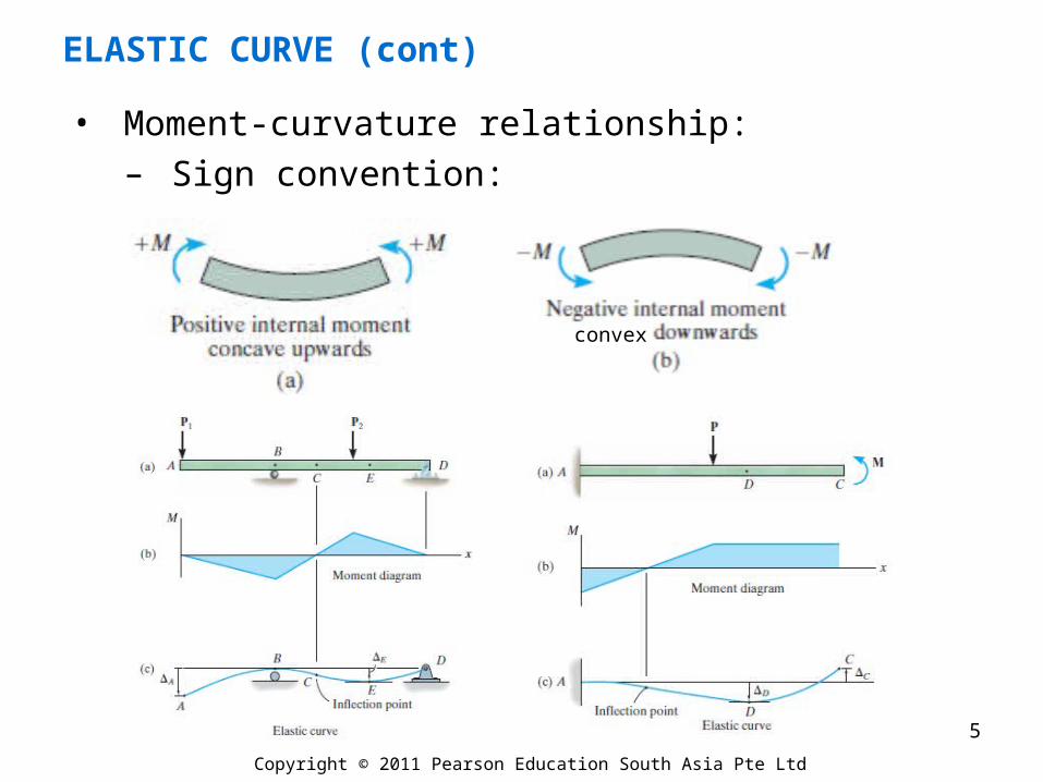
• The deflection diagram of the longitudinal axis that passes through the centroid of each cross-sectional area of the beam is called the elastic curve, which is characterized by the deflection and slope along the curve

4

ELASTIC CURVE (cont)


• Moment-curvature relationship:– Sign convention:

5

convex

ELASTIC CURVE (cont)


• Consider a segment of width dx, the strain in are ds, located at a position y from the neutral axis is ε = (ds’ – ds)/ds. However, ds = dx = ρdθ and ds’ = (ρ-y) dθ, and so ε = [(ρ – y) dθ – ρdθ ] / (ρdθ), or

• Comparing with the Hooke’s Law ε = σ / E and the flexure formula σ = -My/I

y

1

yEEI

M

1

or 1

6

SLOPE AND DISPLACEMENT BY INTEGRATION


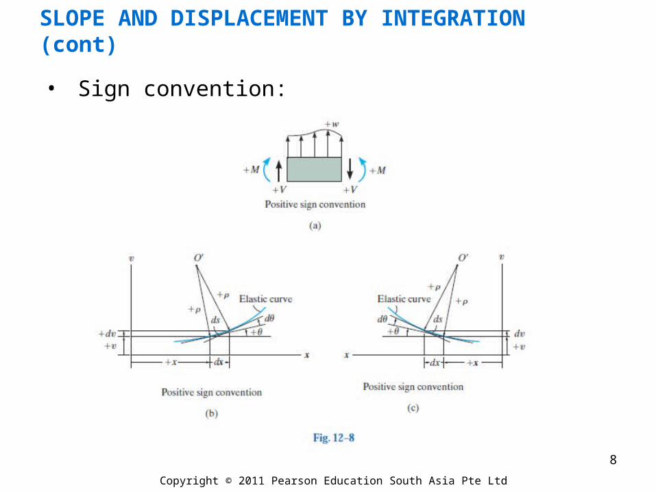
• Kinematic relationship between radius of curvature ρ and location x:

• Then using the moment curvature equation, we have

232

22

1

1

dxdy

dxyd

2

2

2/32

22

1

1

dx

yd

dxdy

dxyd

EI

M

7

SLOPE AND DISPLACEMENT BY INTEGRATION (cont)


• Sign convention:

8

SLOPE AND DISPLACEMENT BY INTEGRATION (cont)


• Boundary Conditions:

– The integration constants can be determined by imposing the boundary conditions, or

– Continuity condition at specific locations

9

EXAMPLE 1


The cantilevered beam shown in Fig. 12–10a is subjected to a vertical load P at its end. Determine the equation of the elastic curve. EI is constant.

10

EXAMPLE 1 (cont)


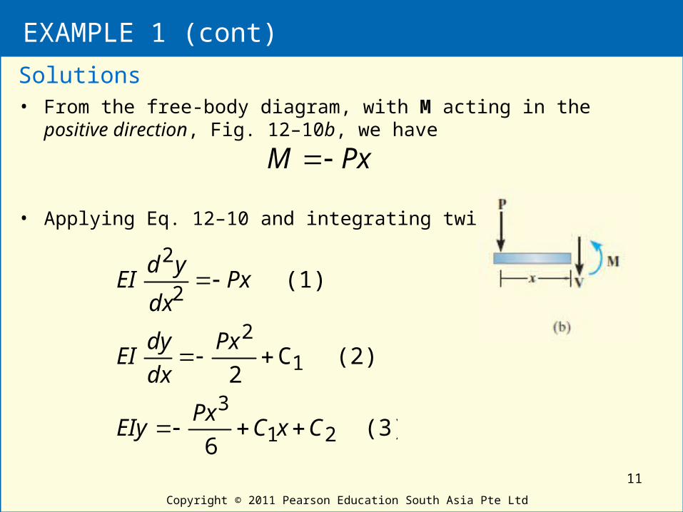
• From the free-body diagram, with M acting in the positive direction, Fig. 12–10b, we have

• Applying Eq. 12–10 and integrating twice yields

Solutions

PxM

(3) 6

(2) C2

(1)

21

3

1

2

2

2

CxCPx

EIy

Px

dx

dyEI

Pxdx

ydEI

11

EXAMPLE 1 (cont)


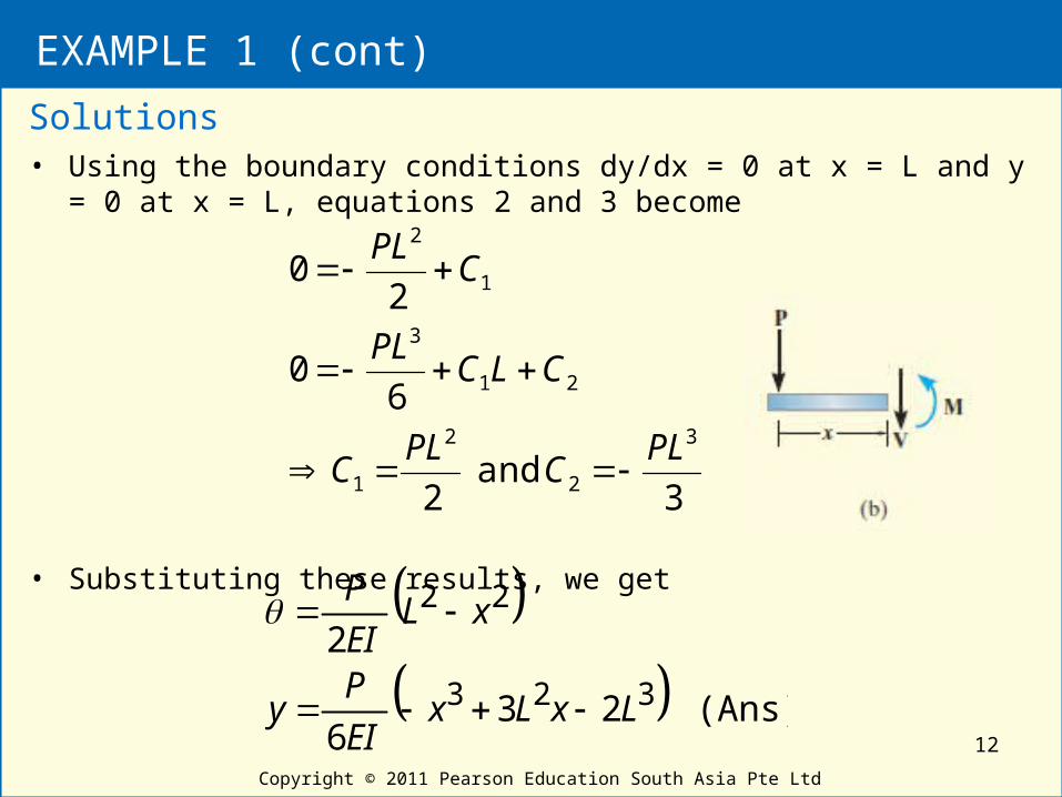
• Using the boundary conditions dy/dx = 0 at x = L and y = 0 at x = L, equations 2 and 3 become

• Substituting these results, we get

Solutions

3 and

2

60

20

3

2

2

1

21

3

1

2

PLC

PLC

CLCPL

CPL

(Ans) 23

6

2

323

22

LxLxEI

Py

xLEI

P

12

EXAMPLE 1 (cont)


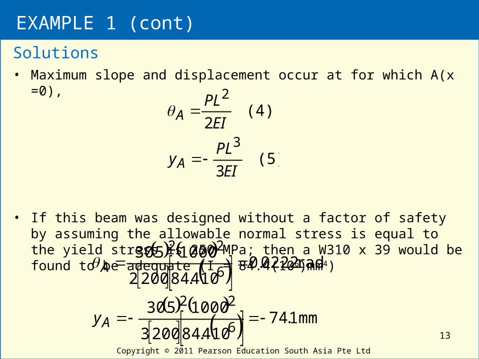
• Maximum slope and displacement occur at for which A(x =0),

• If this beam was designed without a factor of safety by assuming the allowable normal stress is equal to the yield stress is 250 MPa; then a W310 x 39 would be found to be adequate (I = 84.4(106)mm4)

Solutions

(5) 3

(4) 2

3

2

EI

PLy

EI

PL

A

A

mm 1.74

104.842003

1000530

rad 0222.0104.842002

1000530

6

22

6

22

A

A

y

13

EXAMPLE 2


The simply supported beam shown in Fig. 12–11a supports the triangular distributed loading. Determine its maximum deflection. EI is constant.

14

EXAMPLE 2 (cont)


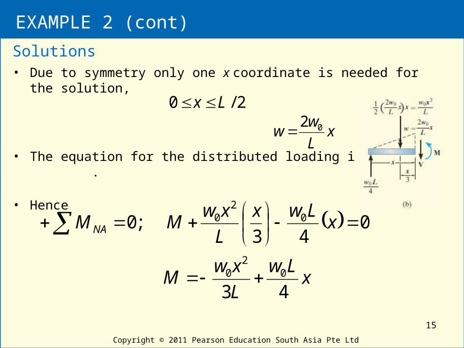
• Due to symmetry only one x coordinate is needed for the solution,

• The equation for the distributed loading is .

• Hence

Solutions

2/0 Lx

xLw

L

xwM

xLwx

L

xwMM NA

43

043

;0

02

0

02

0

xL

ww 02

15

EXAMPLE 2 (cont)


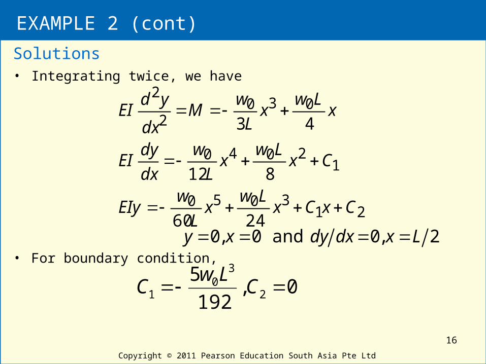
• Integrating twice, we have

• For boundary condition,

Solutions

2,0 and 0,0 Lxdxdyxy 21

3050

12040

0302

2

2460

812

43

CxCxLw

xL

wEIy

CxLw

xL

w

dx

dyEI

xLw

xL

wM

dx

ydEI

0,192

52

30

1 CLw

C

16

EXAMPLE 2 (cont)


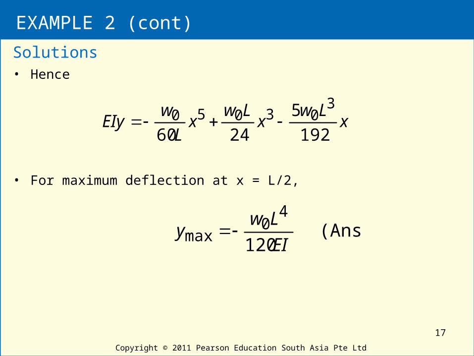
• Hence

• For maximum deflection at x = L/2,

Solutions

(Ans) 120

40

max EI

Lwy

xLw

xLw

xL

wEIy

192

5

2460

303050

17

USE OF CONTINUOUS FUNCTIONS


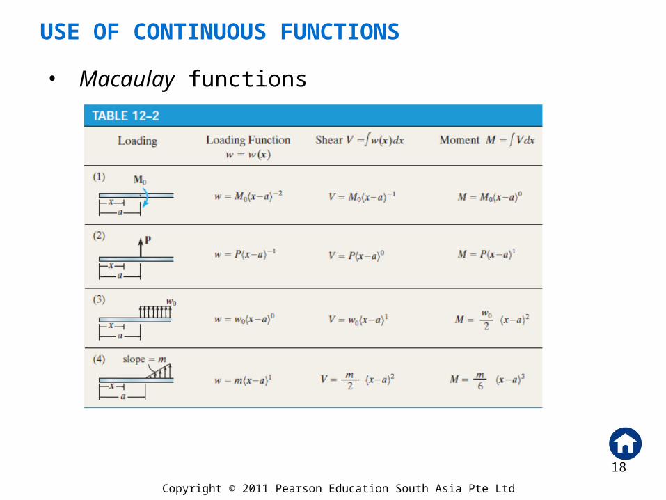
• Macaulay functions

18

USE OF CONTINUOUS FUNCTIONS


• Macaulay functions

• Integration of Macaulay functions:

an

axax

axax

n

n

for

for 0

Cn

axdxax

nn

1

1

19

USE OF CONTINUOUS FUNCTIONS (cont)


• Singularity Functions:

axP

axaxPw

for

for 01

axM

axaxMw

for

for 0

0

2

0

20

USE OF CONTINUOUS FUNCTIONS (cont)


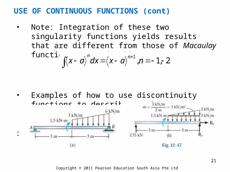
• Note: Integration of these two singularity functions yields results that are different from those of Macaulay functions. Specifically,

• Examples of how to use discontinuity functions to describe the loading or internal moment in a beam:

:

2,1,1

naxdxaxnn

21

EXAMPLE 3


Determine the maximum deflection of the beam shown in Fig. 12–18a. EI is constant.

22

EXAMPLE 3 (cont)


• The beam deflects as shown in Fig. 12–18a. The boundary conditions require zero displacement at A and B.

• The loading function for the beam can be written as

Solutions

1110608

xxw

23

EXAMPLE 3 (cont)


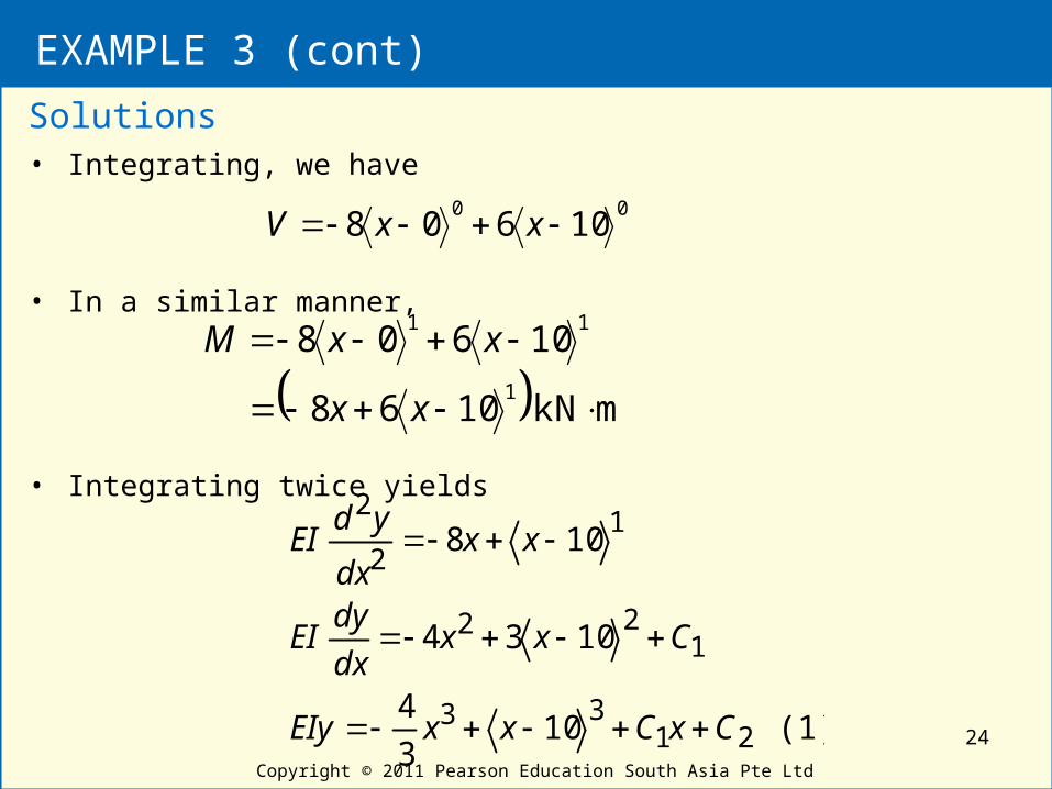
• Integrating, we have

• In a similar manner,

• Integrating twice yields

Solutions

0010608 xxV

mkN 1068

106081

11

xx

xxM

(1) 103

4

1034

108

2133

122

12

2

CxCxxEIy

Cxxdx

dyEI

xxdx

ydEI

24

EXAMPLE 3 (cont)


• From Eq. 1, the boundary condition y = 0 at x = 10 m and at x = 30 m gives

• Thus,

Solutions

12000 and 1333

301030360000

10101013330

21

213

213

CC

CC

CC

(3) 120001333103

4

(2) 13331034

33

22

xxxEIy

xxdx

dyEI

25

EXAMPLE 3 (cont)


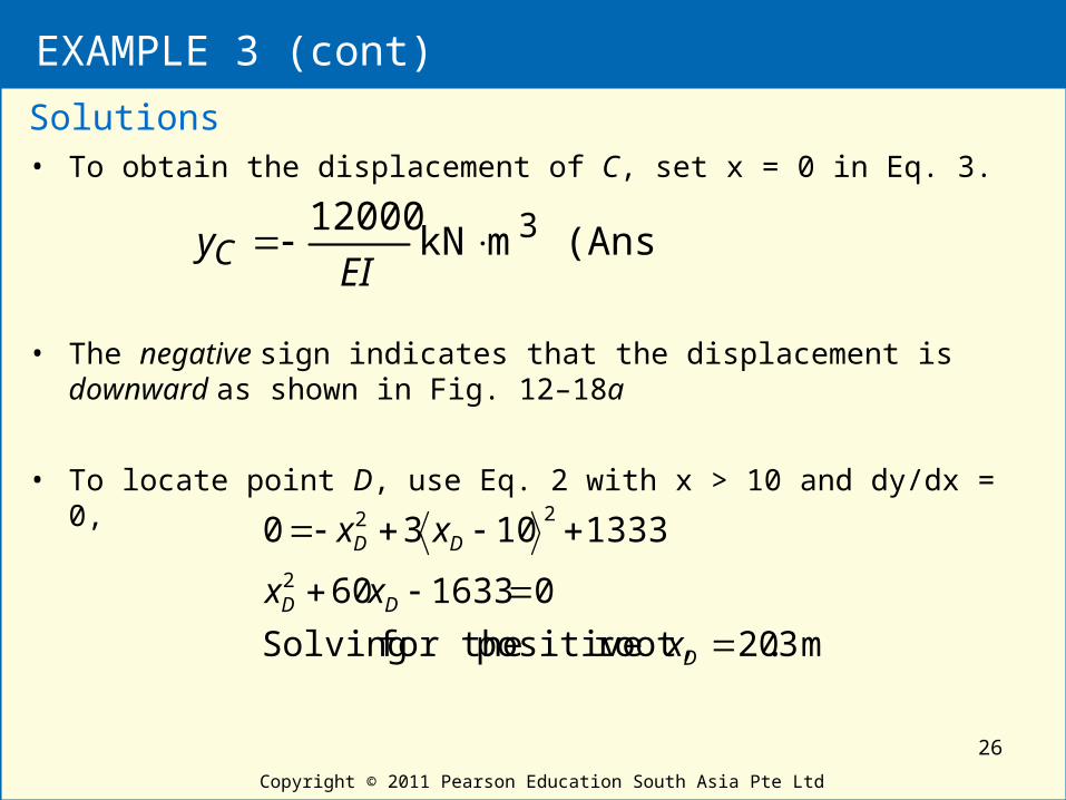
• To obtain the displacement of C, set x = 0 in Eq. 3.

• The negative sign indicates that the displacement is downward as shown in Fig. 12–18a

• To locate point D, use Eq. 2 with x > 10 and dy/dx = 0,

Solutions

(Ans) mkN 12000 3EI

yC

m 320 root, positive for the Solving

0163360

133310302

22

.x

xx

xx

D

DD

DD

26

EXAMPLE 3 (cont)


• Hence, from Eq. 3,

• Comparing this value with vC, we see that ymax = yC.

Solutions

3

33

mkN 5006

120003.201333103.203.203

4

EIy

EIy

D

D

27

EXAMPLE 4


Determine the equation of the elastic curve for the cantilevered beam shown in Fig. 12–19a. EI is constant.

28

EXAMPLE 4 (cont)


• The boundary conditions require zero slope and displacement at A.

• The support diagram reactions at A have been calculated by statics and are shown on the free-body,

Solutions

020215855000258052

xxxxxw

29

EXAMPLE 4 (cont)


• Since

• Integrating twice, we have

Solutions

VdxdMxwdxdV and

1111058550080258052

xxxxxV

mkN 54550452258

582

155008

2

10520258

202

20210

xxxx

xxxxxM

2142432

13132

2022

2

53

1525

3

1

3

26129

53

4550

3

426258

54550452258

CxCxxxxxEIy

Cxxxxxdx

dyEI

xxxxdx

ydEI

30

EXAMPLE 4 (cont)


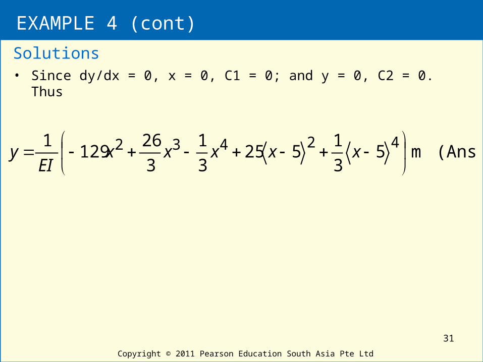
• Since dy/dx = 0, x = 0, C1 = 0; and y = 0, C2 = 0. Thus

Solutions

(Ans) m 53

1525

3

1

3

26129

1 42432

xxxxxEI

y

31

STATISTICALLY INDETERMINATE BEAMS AND SHAFT


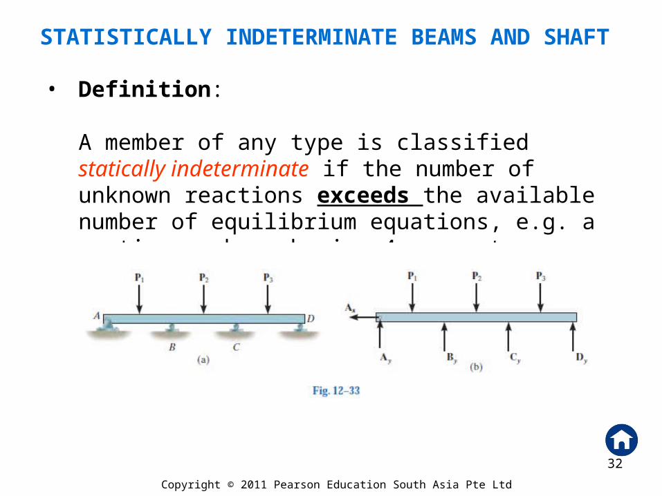
• Definition:

A member of any type is classified statically indeterminate if the number of unknown reactions exceeds the available number of equilibrium equations, e.g. a continuous beam having 4 supports

32

STATISTICALLY INDETERMINATE BEAMS AND SHAFT (cont)


Strategy:

• The additional support reactions on the beam or shaft that are not needed to keep it in stable equilibrium are called redundants. It is first necessary to specify those redundant from conditions of geometry known as compatibility conditions.

• Once determined, the redundants are then applied to the beam, and the remaining reactions are determined from the equations of equilibrium.

33

EXAMPLE 5 – USE OF THE INTEGRATRION METHOD


The beam is subjected to the distributed loading shown in Fig. 12–34a. Determine the reaction at A. EI is constant.

34

EXAMPLE 5 (cont)


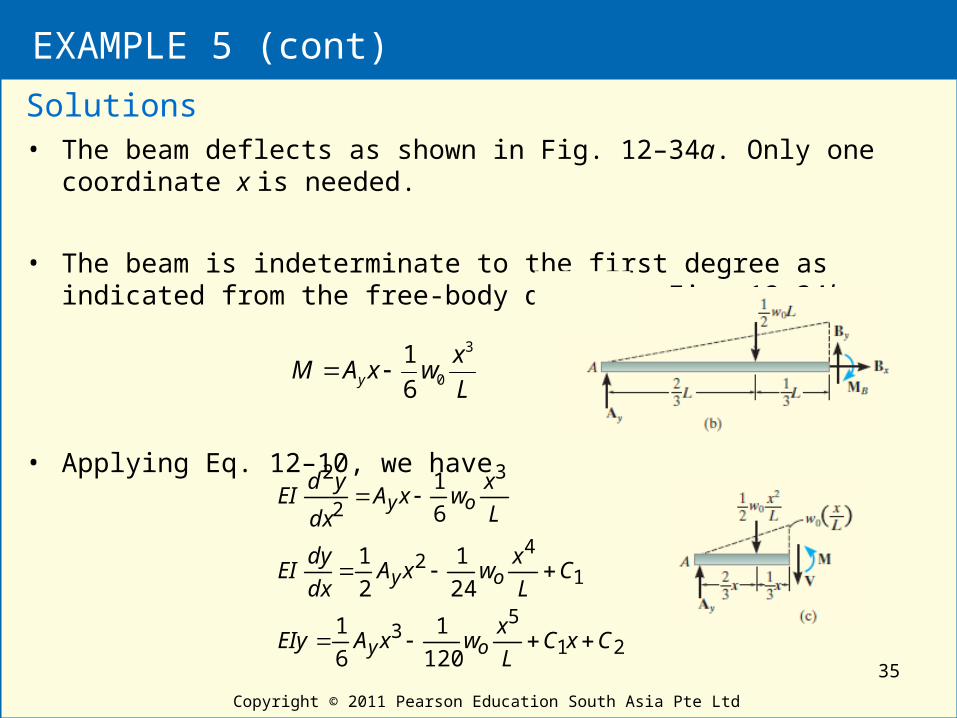
• The beam deflects as shown in Fig. 12–34a. Only one coordinate x is needed.

• The beam is indeterminate to the first degree as indicated from the free-body diagram, Fig. 12–34b

• Applying Eq. 12–10, we have

Solutions

L

xwxAM y

3

06

1

21

53

1

42

3

2

2

120

1

6

1

24

1

2

1

6

1

CxCL

xwxAEIy

CL

xwxA

dx

dyEI

L

xwxA

dx

ydEI

oy

oy

oy

35

EXAMPLE 5 (cont)


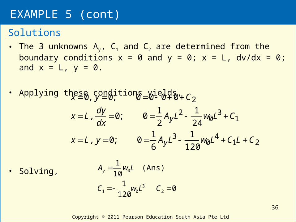
• The 3 unknowns Ay, C1 and C2 are determined from the boundary conditions x = 0 and y = 0; x = L, dv/dx = 0; and x = L, y = 0.

• Applying these conditions yields,

• Solving,

Solutions

214

03

13

02

2

120

1

6

10 ;0 ,

24

1

2

10 ;0 ,

0000 ;0 ,0

CLCLwLAyLx

CLwLAdx

dyLx

Cyx

y

y

0 120

1

(Ans) 10

1

23

01

0

CLwC

LwAy

36

USE OF THE METHOD OF SUPERPOSITION


Procedures:

Elastic Curve

• Specify the unknown redundant forces or moments that must be removed from the beam in order to make it statistically determinate and stable.

• Using the principle of superposition, draw the statistically indeterminate beam and show it equal to a sequence of corresponding statistically determinate beams.

37

USE OF THE METHOD OF SUPERPOSITION (cont)


Procedures:

Elastic Curve (cont)

• The first of these beams, the primary beam, supports the same external loads as the statistically indeterminate beam, and each of the other beams “added” to the primary beam shows the beam loaded with a separate redundant force or moment.

• Sketch the deflection curve for each beam and indicate the symbolically the displacement or slope at the point of each redundant force or moment.

38



Procedures:

Compatibility Equations

• Write a compatibility equation for the displacement or slope at each point where there is a redundant force or moment.

• Determine all the displacements or slopes using an appropriate method as explained in Secs. 12.2 through 12.5.

39



Procedures:

Compatibility Equations (cont)

• Substitute the results into the compatibility equations and solve for the unknown redundant.

• If the numerical value for a redundant is positive, it has the same sense of direction as originally assumed. Similarly, a negative numerical value indicates the redundant acts opposite to its assumed sense of direction.

40



Procedures:

Equilibrium Equations

• Once the redundant forces and/or moments have been determined, the remaining unknown reactions can be found from the equations of equilibrium applied to the loadings shown on the beam’s free body diagram.

41

EXAMPLE 6


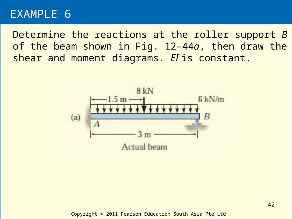
Determine the reactions at the roller support B of the beam shown in Fig. 12–44a, then draw the shear and moment diagrams. EI is constant.

42

EXAMPLE 6 (cont)


• By inspection, the beam is statically indeterminate to the first degree.

• Taking positive displacement as downward, the compatibility equation at B is

• Displacements can be obtained from Appendix C.

Solutions

(1) '0 BB yy

EI

B

EI

PLy

EI

PL

EI

wLy

yB

B

33

334

m 9

3'

EI

mkN 25.83

48

5

8

43

EXAMPLE 6 (cont)


• Substituting into Eq. 1 and solving yields

Solutions

kN 25.9

925.830

y

y

BEI

B

EI

44

EXAMPLE 7


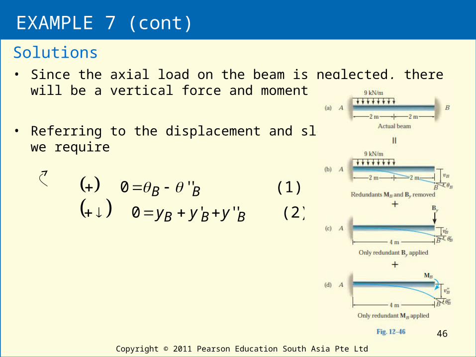
Determine the moment at B for the beam shown in Fig. 12–46a. EI is constant. Neglect the effects of axial load.

45

EXAMPLE 7 (cont)


• Since the axial load on the beam is neglected, there will be a vertical force and moment at A and B.

• Referring to the displacement and slope at B, we require

Solutions

(2) '''0

(1) ''0

BBB

BB

yyy

46

EXAMPLE 7 (cont)


• Use Appx C to calculate slopes and displacements,

Solutions

EI

M

EI

MLy

EI

M

EI

MLEI

B

EI

PLy

EI

B

EI

PL

EIEI

wLy

EI

wL

BB

BB

yB

yB

B

B

8

2''

4''

33.21

3'

8

2'

mkN 42

384

7

EI

mkN 21

48

2

3

2

34

33

47

EXAMPLE 7 (cont)


• Substituting these values into Eqs. 1 and 2 and cancelling out the common factor EI, we get

• Solving these equations simultaneously gives

Solutions

By

By

MB

MB

833.21420

48120

(Ans) mkN 75.3

kN 375.3

B

y

M

B

48

Example 8

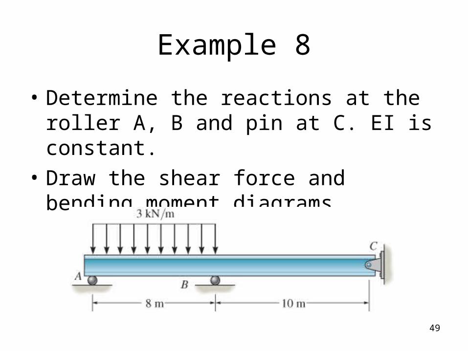
• Determine the reactions at the roller A, B and pin at C. EI is constant.

• Draw the shear force and bending moment diagrams.

49

Example 9

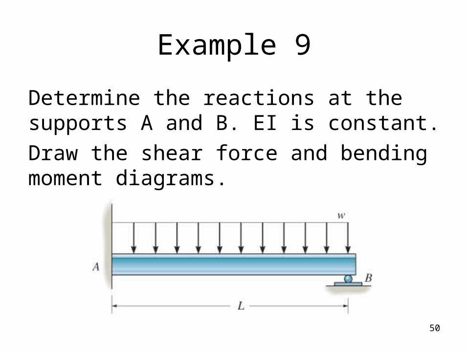
Determine the reactions at the supports A and B. EI is constant.

Draw the shear force and bending moment diagrams.

50

Date post:	21-Dec-2015
Category:	Documents
Upload:	tehpohkee
View:	54 times
Download:	4 times

Deflection of Beams

Documents