www.ivtnetwork.com

Peer Reviewed: Stability

Degradation of Pharmaceutical Solids Accelerated by Changes in Both Relative Humidity and Temperature and Combined Storage Temperature and Storage Relative Humidity (T×h) Design Space for Solid ProductsWilliam R. Porter, Ph.D.

AbstractAchieving stability by design for solid products requires, as one component, the exploration and establishment of boundaries for a storage temperature × relative humidity design space within which the kinetics of degradation of a solid drug or drug product can be predicted using an extended Arrhenius model for the dependence of reaction rates or, equivalently, shelf life on a combined function of both relative humidity and reciprocal absolute temperature. Practical considerations for the design of combined thermal and relative humidity stress degradation experiments and a detailed explanation of proper data analysis methods are defined and illustrated.

Key points include the following:• Achieving stability of both the drug substance

and drug products is a key quality goal. Although thermal stress degradation experiments are a key tool for product development teams to achieve this goal for liquid products and drug substances in solution, the role of relative humidity and its interaction with thermal stress must be studied to understand and predict the degradation kinet-ics of solid drug substances and solid drug prod-ucts, such as tablets or capsule dosage forms.

• A combined storage temperature and relative hu-midity design space can be constructed based on the realization that the drug substance retest date or drug product shelf life is dependent on a func-tion of both the storage temperature and stor-age relative humidity. These effects can be mea-sured experimentally under different conditions of thermal and relative humidity-induced stress. The existence of a combined storage temperature and relative humidity design space is implicit in current stability guidelines.

• Thermal and relative humidity conditions that result in a physical change of state, such as melting or hy-

dration/dehydration, bound the combined storage temperature and storage relative humidity design space. The kinetics of degradation can be predicted successfully for any combination of relative humidity and temperature values within the boundaries of this design space using an extended Arrhenius model for the combined effect of absolute temperature and rela-tive humidity on chemical kinetics.

• The concept of mean kinetic temperature and the re-lated concept of mean kinetic relative humidity are special cases of a more general concept that a set of temperature and relative humidity pairs of points exist such that the extent of degradation is the same for every combination of temperature and relative hu-midity values that lie on this line segment in the tem-perature × relative humidity design space.

• Determining time-to-failure (shelf-life) under accel-erated conditions is all that is necessary to project time-to-failure under other conditions independent of mechanism or kinetic rate constant evaluation. The actual rate of degradation obtained using any particular kinetic model is not required. Straightfor-ward application of an expanded Arrhenius model that includes both the effects of reciprocal absolute temperature and relative humidity under isoconver-sional conditions leads to efficient designs for stress degradation experiments that combine the effects of both factors.

• Once a set of temperature and relative humidity stress degradation experimental conditions have been de-fined that are predictive of degradation under less stressful (normal storage) conditions, experiments using these defined stress conditions can be used routinely to test future batches to predict their sta-bility properties or to verify that process changes do not adversely affect stability properties of the product.

Journal of Validation Technology Volume 19 Number 2

William R. Porter, Ph.D.IntroductionAs noted in a previous report (1), achieving quality by design (QbD), rather than by testing to demonstrate compliance with specifications, is a concept in quality assurance that evolved in the last decade of the twentieth century (2). To recapitulate, quality by design is a key component of the US Food and Drug Administration initiative, Pharmaceutical Current Good Manufacturing Practices (cGMPs) for the 21st Century, announced in August, 2002 (3). These principles have been captured in International Conference for Harmonisation (ICH) guidelines Q8, Q9, Q10, and Q11 (4-7) as well as in the recent FDA guidance on process validation (8). The key to successful development of a quality product by design is the early identification of critical quality attributes as well as ways and means to control and predict them. According to ICH Q11, achieving stability of the drug substance and of products containing the drug substance is a key quality goal. Formal evaluation of drug substance and drug product stability was among the first issues addressed in compilation of the ICH guidelines (9-12). Buried in these guidelines are suggestions that preliminary evaluation of stability properties should include stress degradation studies. However, the nature of these studies is left to the imagination and ingenuity of the innovator. Determining the likely ways in which the final drug product might fail to meet stability expectations and then engineering ways to reduce or prevent these failure modes is the key to achievement of stability by design, and stress degradation experiments are among the most useful tools for evaluating stability failures (13). However, formal guidance on how to perform such studies is lacking, although there have been recent monographs that address this topic (14-16). For solid drug substances and drug products, relative humidity is recognized as one of the key factors influencing stability (9, 14-18).

Storage Temperature and Relative Humidity Design Space and Its relation to Shelf Life for Solid Drug ProductsAs noted previously (1), one of the biggest challenges facing pharmaceutical product developers using the QbD paradigm is that evaluation of stability under ordinary conditions of storage takes time—a lot of time. Recall that the critical quality parameter

of interest for achieving stability by design is the shelf life under the conditions at which the product is stored. The shelf life is simply the elapsed time required for a product that initially met quality expectations to reach the point where it is about to fail meet these expectations as a result of degradation of the product. However, to determine shelf life in accordance with methods described in ICH guidelines (9, 11), one actually has to store the product for the intended shelf life and then verify that it still just barely meets quality expectations. We simply cannot wait until the product fails quality expectations under normal usage; we must somehow devise ways and means to accurately predict the time of failure using methods that take considerably shorter times. For liquid products or for drug substances in solution, methods based on thermal stress and application of the traditional Arrhenius model (19) for the effect of temperature on reaction kinetics can be applied (1). For solid products, the effects of relative humidity also play an important role in determining shelf life (9, 13-18).

By analogy with the approach used for liquid products (1), we must define and explore the boundaries of the design space combining the effects of both storage temperature and storage relative humidity within which the kinetics of degradation of the drug product behave according to a well-defined physicochemical model, so that for any temperature and relative humidity within the design space, we can predict the time to fail to meet stability expectations. The concept of a storage temperature design space is not a new one. It is the unspoken principle underlying the whole field of modern pharmaceutical stability testing that has evolved over the years, culminating in the ICH stability guidelines (9, 11). The concept of a relative humidity design space, especially in combination with storage temperature, is a more recent notion, championed by Waterman and co-workers (20, 21), although based upon a long history of previous work [see, e.g., (17), (18) and references cited therein] that suggested that there exists a range of relative humidity values at each temperature studied for which a relatively simple model could be proposed and found to be predictive for other relative humidity values within the specified range for each temperature. Waterman and co-workers (20, 21) adopted the modified Arrhenius model proposed by Genton and Kesselring (22)

www.ivtnetwork.com

Peer Reviewed: Stabilityas appropriate for the case when only limited degradation is allowed to occur before terminating the experiment. This model had been found to be appropriate for describing the moisture-accelerated degradation of a number of drugs for a range of temperatures (21, 23-27). Other drugs degrade in the presence of moisture in a manner such that this model could be fitted to the experimental data (28). Earlier workers [e.g., (17)] have explored examples in which more extensive degradation was permitted to occur, which is inappropriate for estimating shelf life. In the presence of sufficient moisture, and after sufficient degradation has occurred, the mechanism of degradation changes to one in which sufficient moisture has condensed on the surface of the solid so that subsequent degradation proceeds in the solution that forms in this surface layer (29). By the time this occurs, it is usually the case that too much degradation has already ensued to meet quality expectations (30, 31); models that apply after the product no longer meets stability requirements are outside the scope of this report.As pointed out previously (1), the fundamental concept underlying the ICH guidelines is that there exists a range of storage temperatures within which the degradation rate is a predictable function of the storage temperature following well-established physicochemical principles. Within this range, we can calculate a mean kinetic temperature (32) using the Arrhenius model that faithfully predicts the rate and amount of degradation that may be expected at any given time, based on the thermal history of the sample. The extended Arrhenius model of Genton & Kesselring (22) suggests that just as the simple Arrhenius model can be used to define a mean kinetic temperature at constant relative humidity for which the shelf life would be the same as that observed if the same material were stored on a series of different temperatures actually encountered in the environment in which it is stored and handled, one can also define a mean kinetic relative humidity at constant temperature or a set of equivalent relative humidity and temperature values using the extended Arrhenius model (33). Both heat and humidity accelerate degradation, and the effect is multiplicative. If a drug degrades by some chemical reaction with internal factors (excipients) or external factors (atmospheric oxygen, ionizing radiation), then degradation will not only be faster at higher temperature and/or

higher relative humidity but also be slower at lower temperature and/or lower relative humidity within the temperature and relative humidity range (the storage temperature × relative humidity design space) for which the physicochemical model holds. To increase shelf life, all that is needed is to lower the storage temperature and/or relative humidity, so long as you stay within the storage temperature × relative humidity design space. If a product is exposed transiently to a higher temperature and/or relative humidity combination that is still within the design space, the shelf life will be shortened by a calculable amount. If you know the shelf life at any one particular storage temperature and relative humidity combination with the design space, and you know the physicochemical model relating shelf life to temperature and relative humidity for your drug product that has been demonstrated to be valid within the design space, then it is a simple matter, using the model, to calculate the shelf life at any other combination of temperature, relative humidity, and storage interval at each temperature and relative humidity combination to which the product has been exposed.

Validation that the predictive model actual-ly works within the limits of the design space and definition of those limits as part of the validation process are critical to achieving quality. There may be physical limitations that come into play to limit the storage temperature × relative humidity design space. For example, the mechanism of degradation may change if either the temperature or relative hu-midity is too high. At very high humidity, conden-sation of liquid water on the surface of the material being studied may occur, some of which might the dissolve in this surface layer. Condensation is like-ly to occur readily at low temperatures if humidity is not controlled adequately. Degradation reactions that occur in this solution phase may differ in type and rate from reactions that occur in the solid it-self. Similarly, at high temperatures, other chemi-cal reactions may occur that proceed slowly or not at all at lower temperatures. In addition, changes in physical form, such as formation of hydrates or desolvation of solvates may occur whenever tem-perature or relative humidity boundaries to the de-sign space are crossed. Tablet products containing lubricants such as magnesium stearate dihydrate, for example, will likely show changes in mechanism above the temperature range in which the excipient

Journal of Validation Technology Volume 19 Number 2

William R. Porter, Ph.D.dehydrates at low relative humidity or forms a high-er hydrate at high relative humidity; that is, such products should not be stored above ~70°C. Solid products containing protein substances, in partic-ular, will need to be stored at temperatures below which physical changes in tertiary or quaternary structure occur; thus products formulated in gela-tin capsules should not be exposed to stress above ~50°C. It is important early on to explore a range of storage temperature and relative humidity condi-tions to make sure that the same pattern of degrada-tion is observed throughout the range of conditions studied. For pure drug substances, stress conditions as extreme as 80°C at 75% RH may be acceptable in some cases; other pure substances may show al-tered degradation pathways at 70°C or above. As a general rule, the author has found that for most solid drug substances and prototype formulations storage at 60°C and 75% RH is tolerated. However, limiting conditions must be determined for each new drug substance and for each new combination of excipients used in formulated drug products.

Mean Kinetic Temperature, Mean Kinetic Relative Humidity, and the Equivalent Kinet-ic Temperature-relative Humidity Line Seg-mentThe concept of mean kinetic temperature was intro-duced as a “virtual” temperature by John D. Haynes in 1971 (32). This concept became ingrained in the evaluation of pharmaceutical product stability largely through the writings of Wolfgang Grimm in conjunction with classification of various cities of the world into one of four climatic zones (34-37). Although the concept of mean kinetic temperature was not mentioned in the FDA 1987 stability guide-line (38), it was included in the glossary of terms in the first ICH stability guideline in 1993 (39). The most recent version of this guideline, Q1A(R2) (9), defines the mean kinetic temperature as “A single derived temperature that, if maintained over a de-fined period of time, affords the same thermal chal-lenge to a drug substance or drug product as would be experienced over a range of both higher and lower temperatures for an equivalent defined period. The mean kinetic temperature is higher than the arith-metic mean temperature and takes into account the Arrhenius equation.” The guideline then refers the reader to the original paper by Haynes (32) to es-tablish the mean kinetic temperature for a defined

period. A further definition was adopted by United States Pharmacopeia (USP) as “the single calculated temperature at which the total amount of degrada-tion over a particular period is equal to the sum of the individual degradations that would occur at var-ious temperatures. Thus, MKT may be considered as an isothermal storage temperature that simulates the non-isothermal effects of storage temperature variations. It is not a simple arithmetic mean. MKT is calculated from temperatures in a storage facili-ty.” (40). A formula for computing the mean kinetic temperature has been given in USP that is a slight modification of the original equation proposed by Haynes (41, 42).

TheoryBy combining the original nomenclature proposed by Haynes with the current USP definition, one can define the mean kinetic temperature as:Equation 1:

In Equation 1, Ea represents the Arrhenius acti-vation associated with drug degradation, which is often assumed to be 83.14 kJ/mol (or 19.86 kCal/mol) simply to make the arithmetic easier (42), so that Ea/R = 10,000, where R is the universal gas constant, 0.008314 kJ K–1 mol–1 (0.001986 kCal K–1 mol–1). T1, T2,…,Tn are the average absolute tempera-tures (in Kelvin) during each time period at which the product is stored. For the purposes of compu-tation either the midrange (average of lowest and highest temperature readings during one interval) or the average of multiple temperature readings taken throughout the interval have been proposed (42). Equation 1 assumes that the time intervals for storage at the different temperatures are all equal. The original USP requirement was that temperature be measured monthly for at least 12 months (42), but the concept of mean kinetic temperature can be applied more generally. Thus, one might use weekly or daily or even hourly readings, for example. Coin-cidentally, the “typical” activation energy assumed in the absence of other evidence is very close to the mean activation energy (83 kJ mol–1 or 19.8 kCal/mol) reported by Kennon for 38 drugs and excip-ients reported in the literature between 1950 and

www.ivtnetwork.com

Peer Reviewed: Stability1964 (43) and is also close to the average (82.8 kJ mol–1 or 19.79 kCal/mol) later reported by Grimm and Schepky (44), so it is a reasonable choice in the absence of actual experimental data (45).

Although Equation 1 is based on the Arrhenius model for the dependence of reaction rates on temperature (19), it ignores the effect of relative humidity, which was shown by Genton and Kesselring (22) to also exert a temperature-dependent-effect on reaction rates for the degradation of solids:

Equation 2:

As noted above, the model describe by Equation 2 has been confirmed recently by other investiga-tors (20, 23-27). The rate is also dependent on the reaction mechanism g, which for solids can be com-plex (46-49). However, the choice of reaction mech-anism only affects the value of the pre-exponential factor Ag in Equation 2. Typically B ranges from 0.01–0.09%–1 when h is expressed as 0–100% relative humidity; the median of 15 values reported in the literature was 0.04%–1 (21). More recent studies by Pfizer scientists (42) suggest that many small mol-ecule drugs may have higher Arrhenius activation energies than assumed as the USP default. When Arrhenius activation energies and relative humidity sensitivities for 60 Pfizer development candidates were tabulated (50), the Arrhenius activation en-ergies ranged from 62 to 170 kJ mol–1 with an aver-age Ea = 123.4 kJ mol–1. The relative humidity sensi-tivity ranged from 0 to 0.15 %–1 with an average B = 0.043 %–11.

Equation 3:

This integrates to:

Equation 4:

For solid state reactions, the fraction degraded at a particular time t, α(t), is commonly measured instead of concentration, where:

Equation 5:

For solids, the initial concentration is assumed to be 1 (unity), so the pseudo-zero order model then becomes:

Equation 6:

Despite the documented complexity of solid state degradation reactions, the conventional assumption used by many workers in the pharmaceutical industry is that degradation of solid pharmaceutical products proceeds by a simple process that can be represented by Equation 6 or a similar simple function of storage time.

The models described by Vyazovkin and Wight (46) lead to more complicated behavior. Thus Equation 6 must be modified (see Table I, right-most column).

Diffusion-controlled reaction mechanisms have been proposed to describe the degradation of lyo-philized powders, such as insulin (51), while nucle-ation reactions play a role in photochemical degra-dation and oxidation reactions covered by the scope of this report as well as reactions caused by physical changes, such as desolvation, which are outside the scope of this report (49, 52).

It is trivial to demonstrate by numerical approximation that the fraction degraded as a function of time (except for the Prout-Tompkins model) can be approximated by a simple power function of elapsed storage time in the limit where degradation is small (Table I, right-most column):

Equation 7:

Journal of Validation Technology Volume 19 Number 2

William R. Porter, Ph.D.

Modela Type Integral form g(α) = kt

α(t) Limit as α 0

1-D Diffusion (D1) Diffusion

α2 (kt)(1/2)

2-D Diffusion (D2)Diffusion

[(1 – α)ln(1 – α)] + α (2kt)(1/2)

3-D Diffusion-Jander (D3)Diffusion

[1 – (1– α)(1/3)]2 (9kt)(1/2)

Ginstling-Brounshtein (D4) Diffusion 1 – (2α/3) – (1-α)(2/3) (9kt)(1/2)

Contracting line (R1) Geometrical contraction α kt

Contracting area (R2) Geometrical contraction 1 – (1 – α)(1/2) kt/2Contracting volume (R3) Geometrical contraction 1 – (1 – α)(1/3) kt/3

Zero-order (F0) Reaction-order α kt

First-order (F1) Reaction-order –ln(1 – α) kt

Second-order (F2) Reaction-order (1 – α)–1 – 1 ktThird-order (F3) Reaction-order 0.5 [(1 – α)–2 – 1] ktPower law (P2) Nucleation α(1/2) k2t2

Power law (P3) Nucleation α(1/3) k3t3

Power law (P4) Nucleation α(1/4) k4t4

Avarami-Erofeyev (A2) Nucleation [–ln(1 – α) ](1/2) k2t2

Avarami-Erofeyev (A3) Nucleation [–ln(1 – α) ](1/3) k3t3

Avarami-Erofeyev (A4) Nucleation [–ln(1 – α) ](1/4) k4t4

Prout-Tompkins (B1) Nucleation ln[α/(1 – α)] + cb –∞

a. See reference (47), Table 1.

The exponent r = ½ for diffusion-controlled mod-els, r = 1 for simple geometrical contraction and models reaction order, and r = 2, 3, or 4 for nucle-ation models. Of course, if the reaction is allowed to proceed further, the kinetic behavior becomes more complex. However, these empirical approximations serve well when degradation is limited to the small fraction proposed in the ICH guideline for impuri-ties (30, 31).

Thus, the fractional degradation of a solid, which depends on the reaction mechanism g (which in turn determines r), the relative humidity h, and the absolute temperature T can be expressed (for con-stant h and T) as:

Equation 8:

The fraction degraded (α) at any time t can be calculated using Equation 8 so long as the relative humidity h and the absolute temperature T remain constant. However, if either of these changes, then the calculation must begin afresh at the time of a step change in either T or h:

Table I: Solid-state Rate Expressions for Different Reaction Models.

www.ivtnetwork.com

Peer Reviewed: Stability

More generally,

Equation 10:

Note that if r = 1, then the amount of degradation that occurs in the ith interval ∆ti during which h and T are held constant is:

Equation 11:

Note, in particular, that Equation 11 holds only if r = 1. Equation 10, on the other hand, holds regardless of the interval between successive time readings. To determine the amount of degradation that will occur in the next time interval ∆t, since the change in deg-radation with respect to time is constant when r = 1, it is not necessary to know how much time has elapsed since degradation began. For any other value of r, the amount of degradation occurring in any particular time interval depends upon not only the width of the time interval itself, ∆t, but also on how much time has elapsed, because the change in degradation with respect to time is a function of the elapsed storage time when r ≠ 1.

The ICH definition for mean kinetic temperature is worded in such a way that only the fraction de-graded needs to be monitored. In particular, noth-ing is said about degradation mechanisms or kinetic models. Thus, the ICH definition for mean kinetic temperature can be applied to Equation 10 assum-ing h is zero, and, after solving for the mean kinetic temperature, common elements are factored out:

Equation 12:

Equation 12 is valid for any type of degradation model described in Table I, wherever the approxi-mation described in Equation 7 is valid.In the same manner in which a mean kinetic tem-perature is defined, one can also define a mean ki-netic relative humidity for fixed temperatures as a single derived relative humidity, that if maintained over a defined period of time at a particular tem-perature, affords the same humidity challenge to a drug substance or drug product as would be expe-rienced over a range of both higher and lower rela-tive humidity for an equivalent defined period (33). After factoring out common elements, we obtain:

Equation 13:

Note that Equation 13 is generalized from (Eq. 5) of reference (33) to allow for all of the possible solid state degradation kinetic models. We can combine Equation 12 and Equation 13 to allow both T and h to vary; then there is a set of points on a curve in the T×h plane that satisfies:

Equation 14:

Equation 9:

Again, Equation 14 is generalized from (Eq. 6) of reference (33) to allow for all of the possible solid state degradation kinetic models. There is no unique solution to Equation 14 that simultaneous-ly defines both a mean kinetic temperature and a mean kinetic relative humidity; instead, there are pairs of values in the T×h design space lying on a curved line segment any of which can be selected so long as 0% ≤ h ≤ 100%. Any one of these (T,h) points on this curve will provide equivalent total degrada-tion. That is, T can be changed to compensate for a change in h, and vice versa, to achieve the same overall amount of degradation. Recall that as T de-creases, h increases if the vapor pressure of water is kept constant, until the saturation vapor pressure of water is reached, so some means to change the total amount of moisture present is required to fully ex-ploit potential solutions to Equation 14.

Journal of Validation Technology Volume 19 Number 2

William R. Porter, Ph.D.

Equation 15:

In Equation 15, PS is the saturation vapor pressure of water, T is the absolute temperature (in Kelvin), g0 = –2.8365744×103, g1 = –6.028076559×103, g2 = 1.954263612×101, g3 = –2.737830188×10–2, g4 = 1.6261698×10–

5, g5 = 7.0229056×10–10, g6 = –1.8680009×10–13, and g7 = 2.7150305. For any given temperature T, Equation 15 can be used to find the vapor pressure of water such that h = 100%. This may be required if, instead of the relative humidity, the dew point temperature TD has been measured and reported instead. Thus:

Equation 16:

PS can be obtained from Equation 15 using the measured temperature, and PD can be obtained from Equation 15 using the reported dew point tem-perature after converting both to absolute tempera-tures measured in Kelvin.

Equation 14 can be simplified if r = 1 and all of the time intervals are of equal length, so that:

Equation 17:

ti – ti–1 = Δt = constantThen:Equation 18:

Or, after factoring out Δt:Equation 19:

Equation 19 is essentially (Eq. 6) of reference (33). If, in addition, the relative humidity is fixed using a humidstat even though the temperature is varied, then the exponential terms in Bh can also be factored out, and the mean kinetic temperature calculated using Equation 19 is identical to the value calculated using Equation 1 due to Haynes. The original definition proposed by Haynes is a special case of the more general model, Equation 14.

But is the Haynes definition correct, even in this limited case? Equation 14 (and by implication Equation 1) assumes that changes in temperature and relative humidity occur in discrete isothermal isohumid steps, (i.e., that the temperature and rel-ative humidity values used in calculation are con-stant over each time interval). This is likely to be the case for planned experiments in which open dish samples are moved from one stability cham-ber to another, to simulate exposure to extreme conditions of temperature and relative humidity where brief interludes during sample transfer are small enough to be safely ignored and there is no packaging to impede equilibration of the sample with the new environmental conditions. For real world applications in which temperature and rel-ative humidity vary continuously but are sampled at discrete intervals, as, for example, when work-ing with climate data or with samples protected by packaging, this assumption is unlikely to be cor-rect. However, in the limit as the interval between temperature and relative humidity measurements are made increasingly smaller, the impact of fail-ure to meet the assumption of isothermal isohu-mid conditions diminishes. Purists might want to adjust Equation 14 or Equation 1 to reflect this by adjusting the beginning and ending times for each time period to be intermediate between the times at which actual temperature and relative humid-ity measurements are made. This adjustment in the time base using the actual recorded tempera-ture and relative humidity values is approximately equivalent to averaging the temperature and rela-tive humidity readings taken at the beginning and end of the time period (42). Fortunately, climate data records currently usually consist of readings taken at equally-spaced time intervals, so it is sim-ple enough to adjust Equation 14 or Equation 1 to reflect this fact by replacing the time of measure-ment for each reported temperature/relative hu-

The saturation vapor pressure of water can be computed as a function of absolute tempera-ture T by using an empirical model, originally due to Wexler, but with updated coefficients (53):

www.ivtnetwork.com

Peer Reviewed: Stabilitymidity pair with the midpoints of the time intervals bounding the measurement time. In practice, the effects of these corrections using real climate data are small, with shifts in the mean kinetic T×h curve on the order of 1°C for data reported at hourly inter-vals, depending upon the details of how averaging is performed, as this affects both the total exposure time used in the denominator of the logarithm term in Equation 14 and the actual values of the terms summed in the numerator of the logarithm term.

Another point to consider is whether or not a change in reaction mechanism, for example, from diffusion-controlled degradation (r = ½) to geomet-ric contraction (r = 1) or nucleation (r = 2, 3, or 4) has any impact on the mean kineticT×h curve. This can have pronounced effects when planned experiments using stepwise programmed changes in isothermal isohumid storage conditions are performed.

Isoconversional Paradigm: Time to Fail-ure ExperimentsThe time required for a particular product to fail to meet specifications is independent of the reaction pathway, as long as that pathway is not changed during storage (46, 47). However, while the Arrhe-nius energy of activation Ea and the relative humidi-ty sensitivity coefficient B are unaffected by mecha-nism, the Arrhenius frequency factor Ag is impacted by mechanism. Thus, for example, if it is known that a particular solid drug product degrades in such a way that it fails to meet specifications after storage for two years at 25°C and 60% RH, the actual time-course of degradation (Figure 1) will appear to be much different for different solid state degradation mechanisms.

In particular, note that diffusion kinetics, where the fraction degraded is proportional to the square root of time, leads to rapid detection and quantifica-tion of the principal degradation product early on, but formation of the degradant tapers off as time elapses. Contrast this with the more commonly en-countered pseudo-zero-order process, where quan-tifiable degradant does not typically appear until a significant portion of the shelf life has elapsed. Nucleation kinetics leads to further delays in the appearance of the principal degradation product—much later for a quadratic nucleation mechanism than would be expected for a pseudo-zero-order process, with even longer delays for cubic or quartic nucleation reactions. Indeed, higher order nucle-

ation reactions give the appearance of catastrophic failure with no degradation even detectable until late in the proposed shelf life; product designs that give rise to such failure modes are likely to be weed-ed out during process development.

As an aside, in most cases analytical noise makes it difficult, if not impossible, to distinguish be-tween reactions that proceed by a square root of time dependence (diffusion mechanisms) and two-step pseudo-zero-order reaction characterized by a rapid initial phase that consumes small amounts of material (such as material in amorphous regions or crystal defects) followed by a slower phase that con-sumes the remaining bulk material, so long as tem-perature and relative humidity conditions are kept constant. However, as will be demonstrated later, cycling studies produce characteristic degradation profiles for reactions that proceed by diffusion-con-trolled mechanisms that show repeating patterns of initial rapid growth in degradants followed by slow-er growth over time that recur every time the iso-thermal isohumid conditions are altered.Knowing that time-to-failure does not depend on solid state kinetic mechanism means that forced degradation studies conducted early in the product development process can accurately predict both the extent and general type of mechanism of fail-ure by monitoring the time-course for the appear-ance of degradants. For example, we might consider a drug product with Arrhenius energy of activa-tion Ea = 83.1432 kJ mol–1 (the “typical” value used in the USP definition of mean kinetic temperature) and relative humidity sensitivity coefficient B = 0.04 %–1, a typical value based on earlier reports (21). The more recent values reported by Pfizer scientists with an average Ea = 123.4 kJ mol–1and relative hu-midity sensitivity B = 0.043 %–1 could be used in-stead (50). Assuming that this product will degrade to the extent that it would fail to meet specifications after storage for two years at 25°C and 60% RH, how long would it need to be stored in a controlled rel-ative humidity chamber using a saturated solution of sodium bromide to control relative humidity to achieve the same amount of degradation? This is a relatively simple calculation, with the results illus-trated in Table II.

Thus, if no physical changes in the drug product occur as the temperature is increased, so that Equa-tion 2 is valid (that is, the product remains with-in its T×h design space), then a stress degradation

Journal of Validation Technology Volume 19 Number 2

William R. Porter, Ph.D.

T, °C T, K h, % RHa exp(Bh-Ea/RT) tfailure, daysb tfailure, daysc

5 278.15 63.5 9.54×10-23 7077.7 22532.420 293.15 59.1 1.22×10-21 1340.9 1774.025 298.15 57.6 2.67×10-21 803.6 809.430 303.15 56.0 5.68×10-21 492.7 381.435 308.15 54.6 1.18×10-20 305.1 183.040 313.15 53.2 2.41×10-20 192.2 90.150 323.15 50.9 9.49×10-20 78.4 22.960 333.15 49.7 3.58×10-19 32.5 6.1

70 343.15 49.7 1.31×10-18 13.6 1.7

80 353.15 51.4 4.80×10-18 5.5 0.5

a. (See, e.g., Reference 54). b. Assuming Ea = 83.1432 kJ mol–1 and B = 0.04 %–1. c. Assuming Ea = 123.4 kJ mol–1 and B = 0.043 %–1.

Figure 1: Time Course of Formation of Principal Degradation Product for Different Types of Solid State Reactions.

Table II: Time-to-Failure as a Function of Temperature Using a Sodium Bromide Humidistat.

www.ivtnetwork.com

Peer Reviewed: Stability

experiment lasting only a short period time at an elevated temperature can predict how the product can be expected to behave under long-term storage conditions.

Note that when the Arrhenius activation energy is larger, the time required to achieve the same frac-tion degraded is much shorter at higher tempera-tures, so much so that for the average compound in the Pfizer study, if the actual shelf life at 25°C and 60 %RH were two years, then the shelf life would only be 0.5 days at 80°C. Even if the “typical” activation energy posited by USP is assumed, the shelf life at 80°C would be only 5.5 days for a compound having

this lower activation energy but an actual shelf life at 25°C and 60 %RH equal to two years.

Despite the fact that the relative humidity varies somewhat using a sodium bromide humidistat, an Arrhenius plot of the logarithm of the time-to-fail-ure versus reciprocal absolute temperature is still close to linear (Figure 2).

Note that, in Figure 2, time-to-failure was calcu-lated independently for diffusion-controlled (r = ½), geometric contraction (pseudo zero-order, r = 1), and quadratic nucleation (r = 2) models and that the points are superimposed, as required, since time-to-failure is independent of mechanism. The

Figure 2: Arrhenius Plot for Time to Failure.

Journal of Validation Technology Volume 19 Number 2

William R. Porter, Ph.D.

Figure 3: Diffusion-controlled Degradation under ICH Recommended Storage Conditions.

www.ivtnetwork.com

Peer Reviewed: Stability

Figure 4: Pseudo-zero Order Degradation under ICH Recommended Storage Conditions.

Journal of Validation Technology Volume 19 Number 2

William R. Porter, Ph.D.

slight curvature reflects the non-constant relative humidity used in this experimental design. A higher Arrhenius activation energy implies a steeper slope.

Long-term Storage Degradation PatternsWhat sort of patterns of degradation can be ex-pected for materials stored under typical stability

protocols (e.g., six months at 40°C and 75% RH, one year at 30°C and 65% RH, two years at 25°C) for a drug product with Arrhenius energy of acti-vation Ea = 83.1432 kJ mol–1 and relative humidity sensitivity coefficient B = 0.04 %–1 or with Arrhe-nius energy of activation Ea = 123.4 kJ mol–1 and relative humidity sensitivity coefficient B = 0.043

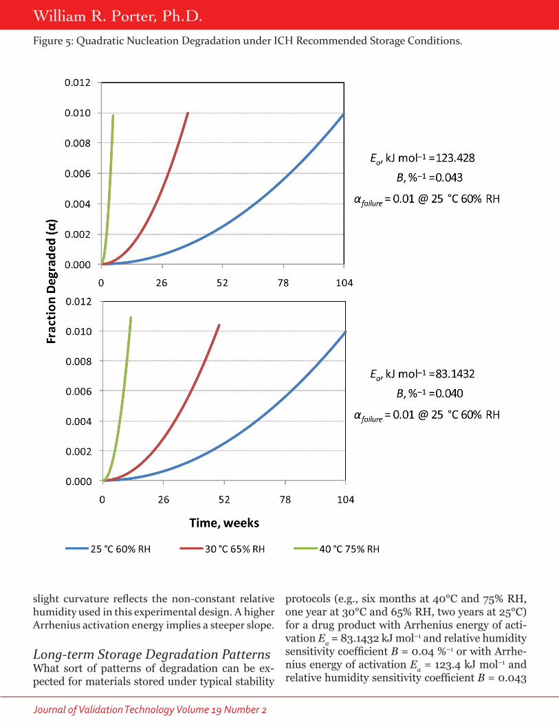
Figure 5: Quadratic Nucleation Degradation under ICH Recommended Storage Conditions.

www.ivtnetwork.com

Peer Reviewed: Stability%–1? As one expects, a diffusion-controlled deg-radation process will exhibit degradant versus time plots that start steeply, but gradually fall off over time (Figure 3), pseudo-zero order reactions have linear degradation versus time plots (Figure 4), while nucleation mechanisms give rise to plots that curve upward (Figure 5).

Note that these patterns remain consistent in shape as the storage temperature and relative hu-midity are varied, so that by studying more carefully the kinetics of degradant formation under acceler-ated conditions, a clearer picture of what to expect at lower temperature and relative humidity condi-tions emerges. Note also that when the Arrhenius activation energy is higher, the time to failure oc-curs earlier at higher temperatures (30 or 40°C) for materials with the same two-year shelf life at 25°C and 60% RH. Thus, for a material with Ea = 123.4 kJ

mol–1 and B = 0.043 %–1, a substance that degrades following pseudo-zero order kinetics will fail to meet specifications after only a little more than five weeks at 40°C and 75% RH, even though it would still meet specifications after storage for two years at 25°C and 60% RH. It would take 12 weeks storage at 40°C and 75% RH for a material with Ea = 83.1432 kJ mol–1 and B = 0.04 if it would also meet specifica-tions after storage for two years at 25°C and 60% RH. Thus, standard stability protocols, such as those in the ICH stability guidelines, may give cause for alarm when drug substances of drug products are tested without prior knowledge of their Arrhenius activation energies and relative humidity sensitivity coefficients.

T °C h, % RH t, days exp(Bh-Ea/RT) αr=½,T,h αr=1,T,h αr=2,T,h

70 75 2 4.43 × 10-12 0.0064 0.0041 0.0016

70 40 2 1.09 × 10-12 0.0032 0.0010 0.0001

60 75 2 1.85 × 10-12 0.0041 0.0017 0.0003

80 40 1 2.50 × 10-12 0.0034 0.0011 0.0001

70 10.8 11 3.40 × 10-13 0.0041 0.0017 0.0003

60 40 11 4.56 × 10-13 0.0048 0.0023 0.0005

50 75 14 7.30 × 10-13 0.0068 0.0047 0.0022

T °C h, % RH t, days exp(Bh-Ea/RT) αr=½,T,h αr=1,T,h αr=2,T,h

70 75 2 4.10 × 10-18 0.0189 0.0358 0.1280

70 40 2 9.09 × 10-19 0.0089 0.0079 0.0063

60 75 2 1.12 × 10-18 0.0099 0.0098 0.0095

80 40 1 3.10 × 10-18 0.0116 0.0135 0.0183

70 10.8 11 2.59 × 10-19 0.0112 0.0124 0.0155

60 40 11 2.48 × 10-19 0.0109 0.0119 0.0142

50 75 14 2.82 × 10-19 0.0131 0.0172 0.0296

Table III: Degradation under ASAP Experimental Design Conditions.

Table IV: Degradation under ASAP Experimental Design Conditions.

Journal of Validation Technology Volume 19 Number 2

William R. Porter, Ph.D.

Accelerated Stability Assessment Program Experimental DesignsExperimental designs for the Accelerated Stability Assessment Program (ASAP) developed by Pfizer scientists (20, 21) to assess the combined effects of relative humidity and storage temperature on drug candidates and drug products using high thermal and relative humidity stress can be evaluated to see the impact of different degradation mechanisms on the amount of degradant that can be expected to be observed. An example for an ASAP design for a drug product with Arrhenius energy of activation Ea = 83.1432 kJ mol–1 and relative humidity sensitivity co-efficient B= 0.04 %–1 is shown in Table III.

Assuming that at least 0.1% (α = 0.001) degrada-tion must occur for quantitation and that at least 0.03% (α = 0.0003) degradation must occur for de-tection, two of the ASAP design p oints in Table III will show no detectable degradation and five will show no quantifiable results if a quadratic nu-cleation degradation reaction were to be operable. All of the experimental design points will produce quantifiable degradation for diffusion-controlled or pseudo-zero order reactions.

An example for an ASAP design for a drug prod-uct with Arrhenius energy of activation Ea = 123.4 kJ mol–1 and relative humidity sensitivity coeffi-cient B = 0.043 %–1 is shown in Table IV.

Assuming that at least 0.1% (α = 0.001) degrada-tion must occur for quantitation and that at least 0.03% (α = 0.0003) degradation must occur for detection, all of the ASAP design points in Table IV will show easily quantifiable degradation for all of the pathways, unlike the results obtained for the lower assumed Arrhenius activation energy used in Table III. It is important to note that the suc-cess of the ASAP experimental plan used in Table III and Table IV depends on the actual Arrhenius ac-tivation energy and relative humidity sensitivity co-efficient for the particular compound being studied, and that the experiment may need to be redesigned if an insufficient number of quantifiable results are obtained on the first attempt. Compounds with low Arrhenius activation energies or low sensitivity to changes in relative humidity will require longer storage times. Fortunately, solution stress degrada-tion experiments are frequently executed prior to degradation studies on solid drug substances and drug products, so adjustments to the design can be

made after simulating results to be expected using information gleaned from previously executed solu-tion stress degradation experiments.

The ASAP design was introduced as a way to screen new small molecule drug candidates (as pure sub-stances) to assess the degree of difficulty that could be encountered during new product development (21). Some of the stress conditions used are clearly too severe for some drug candidates (e.g., biologics) and some drug products (e.g., tablets containing certain lubricants, gelatin capsules). Product devel-opment teams need to design and develop their own version the ASAP experimental design more suited for their own array of potential drug substances or drug products. For example, routine first-in-man solid drug products are typically powders or pow-der-filled capsules that may contain fillers and dis-persing agents or even the components that might eventually be used to manufacture a tablet product. The 70°C and 80°C stress conditions used in the original Pfizer ASAP design are likely too stressful for studying such proposed solid drug products. However, drug product powder blends exposed to 60°C at 75% RH may be stable enough to demon-strate the same pathways for degradation seen under less stressful conditions. Testing at low relative hu-midity and high temperature may cause problems if these conditions result in physical changes to the drug substance or excipients used in formulations, such as dehydration of hydrated crystal forms. So, at least in the initial development stage, careful con-firmation of the identity of physical and polymor-phic forms should be performed. For biologics, even lower thermal stress (45°C or 50°C) may be appro-priate for lyophilized powders containing therapeu-tic proteins or diagnostic protein-based reagents. Development teams need to tailor experimental de-signs to suit their own needs, rather than relying on off-the-shelf canned protocols. For every substance that can be subjected to formal evaluation of stabil-ity in accordance with ICH guidelines there does in fact exist a storage temperature × relative humidity design space, the boundaries of which differ from drug substance to drug substance and drug prod-uct to drug product. The sooner these boundaries are defined in the product development process, the easier subsequent development steps can be com-pleted successfully.

www.ivtnetwork.com

Peer Reviewed: StabilityIsothermal Isohumid Cyclic Excur-sion Designs Consider next the evaluation of ki-netic data for an experiment in with a drug product, assuming again that the Arrhenius energy of activation is ei-ther Ea = 83.1432 kJ mol–1 and relative humidity sensitivity coefficient B = 0.04 %–1 or Ea = 123.4 kJ mol–1 and relative hu-midity sensitivity coefficient B = 0.043 %–1, but this time that the material fails to meet specifications after storage at 25°C and 60% RH after only one year. The product, stored in an open dish exposed to the atmosphere in the test chamber, is subjected to three cycles of exposure to temperature and rela-tive humidity extremes, first to 50°C at 75% RH for one week, then to 5°C at 75% RH for three weeks. The cycle is repeated a total of three times, then beginning with week 13, the materi-al is stored at 25°C and 60% RH for 18 weeks. The product is then subjected to one more cycle of exposure to the same

temperature and relative humidity extremes followed by another 18 weeks of storage at 25°C and 60% RH for 18 weeks. The entire experiment takes 52 weeks (one year) to complete. What does the degradation pro-file look like? What would the degradation profile look like if instead the product were stored under conditions of equivalent ki-netic temperature and relative humidity for the same interval? What combinations of temperature and relative humidity would be feasible to use that satisfy the requirements for equivalent kinetic temperature and rela-tive humidity as defined using Equation 14?

These questions are easily answered by simulating the data that would be obtained and plotting the results (Figure 6, Figure 7, and Figure 8).

It is important to note, especially in Fig-ure 6 and Figure 8, that the “clock starts over at zero” whenever a step change in tempera-ture and relative humidity conditions oc-curs. The rate of change of the fraction de-

Figure 6: Cyclic Exposure Experiment for a Diffusion-controlled Degradation Process.

Figure 7: Cyclic Exposure Experiment for a Pseudo-zero Order Degradation Process.

Journal of Validation Technology Volume 19 Number 2

William R. Porter, Ph.D.

Note: Measured data from reference (55).

graded with respect to a change in stor-age time is a function of the time that has elapsed since the most recent step change. This is not relevant for pseu-do-zero order reactions, as displayed in Figure 7, because the rate of change in fraction degraded is independent of the elapsed storage time in this case.

It is always possible, using Equation 14, to find a set of temperature and relative humidity values that will pro-duce equivalent degradation over the total time course of the experiment. For diffusion-controlled degradation reactions, the equivalent kinetic tem-perature and relative humidity pairs that provide equivalent degradation will always be higher than those that would be obtained if the reaction were to follow pseudo-zero order kinetics. Likewise, for power law nucleation ki-netics reactions, the equivalent kinetic

Figure 8: Cyclic Exposure Experiment for a Quadratic Nucleation Degradation Process.

Figure 9: Hourly Temperature and Relative Humidity for Santa Rosa, California, in 2010.

temperature and relative humidity pairs that provide equivalent deg-radation will always be lower than those that would be obtained if the reaction were to follow pseudo-zero order kinetics.

Equivalent Kinetic Tempera-ture and Relative Humidity for a Geographic Location The dependence of degradation rate on the elapsed time since the most recent step change in temperature and relative humidity illustrated above for a planned excursion ex-periment poses a problem if we desire to define equivalent kinetic temperature-relative humidity pairs for a geographical location based upon climate data. Clearly, in the real world, temperature and relative humidity are in constant flux. What is needed is a form of Equation 14 in which the time intervals are small, equal in length, and for which the

www.ivtnetwork.com

Peer Reviewed: Stabilityfraction degraded is independent of elapsed stor-age time. This can only be achieved if we assume pseudo-zero-order kinetics. If that were true, then Equation 19 holds, and a set of equivalent kinetic temperature and relative humidity values can be de-fined based on climate data.The dependence of degradation rate on the elapsed time since the most recent step change in tempera-ture and relative humidity illustrated above for a planned excursion experiment poses a problem if we desire to define equivalent kinetic temperature-rel-ative humidity pairs for a geographical location based upon climate data. Clearly, in the real world, temperature and relative humidity are in constant flux. What is needed is a form of Equation 14 in which the time intervals are small, equal in length, and for which the fraction degraded is independent of elapsed storage time. This can only be achieved if we assume pseudo-zero-order kinetics. If that were true, then Equation 19 holds, and a set of equivalent kinetic temperature and relative humidity values can be defined based on climate data.

By way of illustration, temperature, and relative humidity data for the city of Santa Rosa, California (55), a location that typically has cool, rainy winters and warm, dry summers, is shown in Figure 9 for a substance which degrades by pseudo-zero-or-der kinetics for which Ea = 83.1432 kJ mol–1 and B = 0.04 %–1 (lower panel) and for which Ea = 123.4 kJ mol–1 and B = 0.043 %–1 (upper panel).

Differences in the assumed values for Ea and B have only a modest effect on the calculated USP mean ki-netic temperature. However, these differences are more pronounced when the mean kinetic T×h curves are compared. Although the higher Arrhenius ac-tivation energy characteristic of the recent Pfizer development candidates results in a higher mean kinetic temperature computed using the USP for-mula, Equation 1, not surprisingly, the mean kinet-ic T×hcurve calculated using Equation 19 spans a narrower range of temperatures than the same curve calculated using the lower Arrhenius activation en-ergy recommended by USP. This reflects the great-er importance of the dependence of degradation on temperature when the Arrhenius activation energy is large compared to the effects of changing relative hu-midity. If there were no effect of relative humidity at all, the T×h curve would collapse to the vertical line that indicates the USP MKT.

For this location, the curve representing joint es-timates of equivalent kinetic temperature and rela-tive humidity using Equation 19 gives a more “typ-ical” average representation of the actual tempera-ture and relative humidity data than can be gleaned from the single mean kinetic temperature estimate obtained by using the USP formula, Equation 1. In particular, note that even in the summer, when tem-peratures occasionally approach 40°C but relative humidity is low, there are only very few instances when the equivalent kinetic temperature and rel-ative humidity curve would be exceeded, whether the USP-suggested Arrhenius activation energy or a higher value is used. Of far greater concern would be unprotected exposure to the external environment on many of those damp, moderately cool days that typically occur in autumn or late spring, when the temperature is close to the USP MKT for this geo-graphical location (and is well below what is likely to be listed on the label for the product), but the rel-ative humidity exceeds 80% RH. For this particular geographical location, protection of moisture-sen-sitive products from exposure to high relative hu-midity in the external environment is likely to be more important for product stability than protec-tion from high temperature.

Stability by Design for Solid Pharmaceuti-cal Substance and Solid Dosage FormsAchievement of stability by design for liquid prod-ucts has been previously discussed (1). All of these measures must still be considered when designing solid products. However, in the case of solid mate-rials, both temperature and relative humidity must be considered jointly in defining a storage condi-tion design space within which experimental re-sults obtained under stress conditions can be used to accurately predict stability-indicating quality parameters under less stressful storage conditions. Stress degradation experiments can not only help the product development determine how shelf life varies with changes in storage temperature and rel-ative humidity but can also provide clues as to the general nature of solid state reaction kinetics that can be expected to be observed in real-time studies conducted according to ICH guidelines. In the au-thor’s experience, diffusion-controlled degradation occurs often enough in practice, so that traditional real-time stability studies systematically underesti-mate shelf life for drug substances and drug prod-

Journal of Validation Technology Volume 19 Number 2

William R. Porter, Ph.D.ucts that exhibit this type of degradation kinetics. Regulatory agencies hold troves of data that could be mined to determine just how frequently this oc-curs in practice. On the other hand, the author is not aware of any drug substances or drug products that exhibit nucleation kinetic behavior that have been successfully marketed. Perhaps the apparent catastrophic failure of such materials late in con-ventional stability programs has deterred approval for marketing. Nevertheless, if the general nature of the kinetics of failure are known and understood, it should be possible to design products that will be able to meet long-term real time stability expecta-tions even if nucleation kinetics are suspected to be involved in principal failure modes. However, con-ventional stability monitoring protocols will need to be modified for such materials, with greater em-phasis on monitoring late stage conformance with stability expectations and requirements.

Early appearance of degradation products will al-ways be impossible to detect because the limit of detection of analytical methods will never be low enough to assure detection at the earliest sampling times. The time required to observe quantifiable degradation may be delayed considerably, depend-ing on the general kinetic pattern observed, with quantifiable degradation observed earlier for those materials that exhibit diffusion-controlled kinetics of solid state degradation than for those following conventionally assumed pseudo-zero-order kinet-ics. Quantifiable degradation may not be observed for materials that degrade by nucleation kinetic mechanisms in the solid state until relatively late in the planned monitoring period. Nevertheless, these concerns will not impede product development if ex-periments to define time-to-failure under conditions of thermal and humid stress are used as a means to explore the storage temperature × relative humidity design space. So long as the analytical method is ca-pable of quantifying the degradation products that would actually indicate failure to conform to quality expectations with sufficient precision, a model can be constructed that will adequately predict time to failure under less stressful conditions. Product de-velopment teams need to learn early in the develop-ment cycle what type of kinetic pattern will be ob-served in later real time stability evaluations, so that more appropriate monitoring times can be defined for pivotal stability evaluations. This can be done by adopting some version of the ASAP experimental

design advocated by Pfizer scientists, although the Pfizer experimental plans may require custom mod-ification to suit individual project goals. Cyclic ex-posure to different stress conditions should always exhibit the same pattern of degradation no matter at what point in the overall planned storage regimen they are actually conducted. Indeed, performing storage condition cycling experiments at different times within an overall storage regimen can provide confirmation that a storage temperature and rela-tive humidity design space has been properly and adequately defined for the drug substance or drug product. With adequate exploration of the storage temperature × relative humidity design space com-pleted early in the development process, the re-sults of formal stability experiments conducted in accordance with ICH guidelines ought to be com-pletely predictable in advance. The formal experi-ments then serve merely to validate the predictions based on stress experiments. Once predictive stress degradation experiments have been designed and their predictive power is verified, these stress pro-tocols can be used routinely to evaluate the effects of process changes on stability as well as to monitor stability properties of individual batches. Finally, if a drug substance or drug product is subjected to storage temperature or relative humidity excursions during warehousing and distribution and if actual temperature and relative humidity conditions to which the material had been exposed prior to the excursion are known, it should be possible to cal-culate the effect on shelf life from knowledge of the set of temperature and relative humidity values that collectively define “equivalent kinetic temperature and relative humidity” conditions used in stability trials. Given this knowledge of the temperature and relative humidity design space, it is possible to cal-culate in advance just how severe an excursion from labeled storage conditions must be in order to com-promise the quality of the product.

References

1. W.R. Porter, “Thermally Accelerated Degradation and the Storage Temperature Design Space for Liq-uid Products,” Journal of Validation Technology 18 (3) 73–92, 2012.

2. J.M. Juran, Juran on Quality by Design: The New Steps for Planning Quality into Goods and Services, New York, NY, The Free Press, 1992.

www.ivtnetwork.com

Peer Reviewed: Stability3. FDA, Pharmaceutical Current Good Manufacturing

Practices (cGMPs) for the 21st Century: A Risk-Based Approach: Final Report (Rockville, MD, Sept. 2004)

4. ICH Q8 (R2) Pharmaceutical Development.5. ICH Q9 Quality Risk Management6. ICH Q10 Pharmaceutical Quality System7. ICH Q11 Development And Manufacture of Drug Sub-

stances8. FDA, Guidance for Industry: Process Validation:

General Principles and Practices (Rockville, MD, Oct. 2011)

9. ICH Q1A(R2) Stability testing of new drug substances and products (second revision)

10. ICH Q1B Stability testing: Photostability testing of new drug substances and products

11. ICH Q1E Evaluation of Stability Data12. ICH Q5C Quality of Biotechnological Products: Sta-

bility Testing of Biotechnological/Biological products13. W.R. Porter, “Stability by Design,” Journal of Valida-

tion Technology 17 (3), 82–96, 2011.14. D. Zhou D, W.R. Porter, G.G.Z. Zhang, “Drug stability

and degradation studies,” In: Y. Qiu, Y. Chen, G.G.Z. Zhang, L. Liu, W.R. Porter, Developing Solid Oral Dosage Forms: Pharmaceutical Theory and Practice, New York: Academic Press–Elsevier, 2009.

15. S.W. Baertschi, Pharmaceutical Stress Testing, Boca Raton, FL, Taylor & Francis Group, 2005.

16. K.C. Waterman, “Understanding and Predicting Pharmaceutical Shelf-life,” In: Huynh-Ba K. Hand-book of Stability Testing in Pharmaceutical Develop-ment: Regulations, Methodologies and Best Practic-es, New York, NY, Springer, §6.4.3, 2009.

17. J.T. Carstensen, Drug Stability Principles and Practic-es, 2nd Ed., Revised and Expanded. New York: Marcel Dekker, ch 10. 281–303, 1995.

18. S. Yoshioka and V.J. Stella, Stability of drugs and dos-age forms, New York, NY, Kluwer Academic/Plenum Publishers, 108–113, 2000.

19. S.A. Arrhenius, “Über die reaktionsgeschwindigheit bei der inversion von rohrzucker durch saüren,” Z Physik Chem 4, 226–248, 1889.

20. K.C. Waterman and R.C Adami, “Accelerated Aging: Predictions of Chemical Stability of Pharmaceuti-cals,” International Journal of Pharmaceutics 293, 101–125, 2004.

21. K.C. Waterman, A.J. Carella, M.J. Gumkowski, P. Lukulay, B.C. MacDonald, M.C. Roy, S.L. Shamblin, “Improved Protocol and Data Analysis for Acceler-ated Shelf-life Estimation of Solid Dosage Forms,” Pharmaceutical Research 24 (4), 789–790, 2007.

22. D. Genton, U.W. Kesselring, “Effect of Temperature and Relative Humidity on Nitrazepam Stability in Solid State,” Journal of Pharmaceutical Science, 66 (5), 676–680, 1977.

23. X.Y. He, G.K. Yin, B.Z. Ma, “A Study on the Decom-position Kinetics of Vitamin C Powder,” Acta Phar-macologica Sinica 25, 543–550, 1990.

24. A. Jelinska, M. Zajac M, J. Gostomska, M. Szczepan-iak, “Kinetics of cefamandole nafate degradation in solid phase,” Il Farmaco 58, 309–313, 2003.

25. K.C. Waterman, “Accelerated aging and oxidation,” Presented at Oxidative Degardation and Stabiliza-tion of Pharmaceuticals Conference, organized by the Institute for International Research, Princeton, NJ, 2004.

26. Q. Zhao, X. Zhan, L. Li, C. Li, T. Lin, X. Yin, N. He, “Programmed humidifying in drug stability exper-iments,” Journal of Pharmaceutical Science 94 (11), 2531–2540, 2005.

27. L.L. Li, X.C. Zhan, and J.L. Tao, “Evaluation of the Stability of Aspirin in Solid State by the Programmed Humidifying and Non-isothermal Experiments,” Ar-chives of Pharmaceutical Research 31 (3), 381–389, 2008.

28. J.T. Carstensen, E.S. Aron, D.C. Spera, J.J. Vance, “Moisture Stress Tests in Stability Programs, Journal of Pharmaceutical Science 55, 561–563, 1966.

29. S. Yoshioka, M. Uchiyama, “Kinetics and Mechanism of the Solid-state Decomposition of Propantheline Bromide,” Journal of Pharmaceutical Science 75, 92–96, 1986.

30. ICH Q3A(R2) Impurities in new drug substances31. ICH Q3B(R2) Impurities in new drug products32. J.D. Haynes, “Worldwide Virtual Temperatures for

Product Stability Testing,” Journal of Pharmaceutical Science 60 (6), 927–929, 1971.

33. G. Scrivens, “Mean Kinetic Relative Humidity: A New Concept for Assessing the Impact of Variable Rela-tive Humidity on Pharmaceuticals,” Pharmaceutical Technology 36 (11), 52–57, 2012.

34. W. Grimm, “Storage Conditions for Stability Testing – Long Term Testing and Stress Tests,” Drugs made in Germany 28, 196–202, 1985.

35. R. Dietz, K. Feilner, F. Gerst, W. Grimm, “Drug Sta-bility Testing – Classification of Countries Accord-ing to Climatic Zone,” Drugs made in Germany 36, 99–103, 1993.

36. W. Grimm, “Storage Conditions for the Most Im-portant Market for Drug Products, Including the EC, Japan and the USA,” Drug Development and Industri-al Pharmacy 19, 2795–2830, 1993.

37. W. Grimm, “Extension of the International Con-ference On Harmonization Tripartite Guideline for Stability Testing of New Drug Substances and Prod-ucts to Countries of Climatic Zones III and IV,” Drug Development and Industrial Pharmacy 24, 313–325, 1998.

Journal of Validation Technology Volume 19 Number 2

William R. Porter, Ph.D.38. FDA, Guideline for submitting documentation for the

stability of human drugs and biologics (Rockville, MD 1987). Reproduced in: J.T. Carstensen, Drug Sta-bility Principles and Practices 2nd Edition, Revised and Expanded, New York, NY, Marcel Dekker, Inc., pp. 551–579, 1995.

39. ICH, Stability testing of new drug substances and products. ICH Harmonised Tripartite Guideline, ICH (1993). Reproduced in: J.T. Carstensen, Drug Stability Principles and Practices 2nd Edition, Revised and Expanded, New York, NY, Marcel Dekker, Inc., pp. 538–550, 1995.

40. USP General Chapter <1150> Pharmaceutical stabil-ity

41. USP General Chapter <1160> Pharmaceutical calcu-lations in prescription compounding.

42. L.C. Bailey, “Mean Kinetic Temperature—A Con-cept for Storage of Pharmaceuticals,” Pharmacopeial Forum 19 (5), 6163–6166, 1993.

43. L. Kennon, “Use of Models in Determining Chemical Pharmaceutical Stability,” Journal of Pharmaceutical Science 53 (7), 815–818, 1964.

44. W. Grimm, G. Schepky, Stabilitatsprufung in der Pharmazie,Theorie und Praxis, Alendorf, Germany: Editio Cantor Verlag, 1980.

45. W. Grimm, “Storage Conditions for Stability Testing in the EC, Japan and the USA, the Most Important Market for Drug Products,” Drug Development and Industrial Pharmacy 19 (20), 2795–2830. 1993.

46. A. Vyazovkin, C.A. Wight, “Kinetics in Solids,” An-nual Review of Physical Chemistry 48, 132–133, 1977.

47. A. Khawam, “Application of solid-state kinetics to desolvation reactions,” Iowa City, IA: The University of Iowa, PhD Thesis, 2007.

48. A. Khawam & D.R. Flanagan, “Solid-state kinetic models: Basics and mathematical fundamentals,” Journal of Physical Chemistry B 110 (35): 17315–17328, 2006.

49. A. Khawam and D.R. Flanagan, “Basics and Applica-tions of Solid-state Kinetics: A Pharmaceutical Per-spective,” Journal of Pharmaceutical Science 95 (3), 472–498, 2006.

50. G. Scrivens, “Accurate Shelf-Life Predictions Using ASAP (Accelerated Stability Assessment Program),” Presented at The Pharmaceutical Analytical Sciences Group 2010 PASG meeting, Milton Keynes, UK May 10–11th (2010).

51. M.J. Pikal and D.R. Rigsbee, “The Stability of Insulin in Crystalline and Amorphous Solids: Observation of Greater Stability for the Amorphous Form,” Phar-maceutical Research 14 (10), 1379–1387, 1997.

52. Z. Qiang, J.H. Chang, C.P. Huang, and D. Cha, “Ox-idation of Selected Polycyclic Aromatic Hydrocar-bons by the Fenton's Reagent: Effect of Major Factors

Including Organic Solvent,” In: Eller PG, Heineman WR eds, Nuclear Site Remediation Washington D.C., American Chemical Society, ACS Symposium 778, pp. 187–209, 2000.

53. M. Zahn, “Global Stability Practices,” In: Huynh-Ba K (Ed), Handbook of Stability Testing in Pharma-ceutical Development: Regulations, Methodologies and Best Practices, New York, NY: Springer Science+ Business Media LLC, pp. 48–49, 2009.

54. OIML R 121, “The Scale of Relative Humidity of Air Certified Against Saturated Salt Solutions,” Paris, France: Organisation Internationale de Métrologie Légale, 1996.

55. California Irrigation Management Information Sys-tem (CIMIS), Data for Santa Rosa, California avail-able online retrieved from: http://wwwcimis.water.ca.gov/cimis/dataInfoType.jsp.

About the AuthorWilliam R. Porter formerly served for more than 25 years in the Pharmaceutics group at Abbott Global Pharmaceutical Research and Development, Abbott Park, Illinois, USA.

www.ivtnetwork.com

Peer Reviewed: Stability