Delft University of Technology

A data-driven surrogate modelling approach for acceleration of short-term simulations of adynamic urban drainage simulator

Mahmoodian, Mahmood; Torres-Matallana, Jairo Arturo; Leopold, Ulrich; Schutz, Georges; Clemens,FrancoisDOI10.3390/w10121849Publication date2018Document VersionFinal published versionPublished inWater (Switzerland)

Citation (APA)Mahmoodian, M., Torres-Matallana, J. A., Leopold, U., Schutz, G., & Clemens, F. H. L. R. (2018). A data-driven surrogate modelling approach for acceleration of short-term simulations of a dynamic urban drainagesimulator. Water (Switzerland), 10(12), [1849]. https://doi.org/10.3390/w10121849

Important noteTo cite this publication, please use the final published version (if applicable).Please check the document version above.

CopyrightOther than for strictly personal use, it is not permitted to download, forward or distribute the text or part of it, without the consentof the author(s) and/or copyright holder(s), unless the work is under an open content license such as Creative Commons.

Takedown policyPlease contact us and provide details if you believe this document breaches copyrights.We will remove access to the work immediately and investigate your claim.

This work is downloaded from Delft University of Technology.For technical reasons the number of authors shown on this cover page is limited to a maximum of 10.

water

Article

A Data-Driven Surrogate Modelling Approach forAcceleration of Short-Term Simulations of a DynamicUrban Drainage Simulator

Mahmood Mahmoodian 1,2,* , Jairo Arturo Torres-Matallana 1,3 , Ulrich Leopold 1 ,Georges Schutz 4 and Francois H. L. R. Clemens 2,5

1 Environmental Informatics Group, ERIN Department, Luxembourg Institute of Science andTechnology (LIST), L-4422 Belvaux, Luxembourg; arturo.torres@list.lu (J.A.T.-M.);ulrich.leopold@list.lu (U.L.)

2 Sanitary Engineering Section, Water Management Department, Faculty of Civil Engineering andGeosciences, Delft University of Technology, 2628 CN Delft, The Netherlands; f.h.l.r.clemens@tudelft.nl

3 Soil Geography and Landscape Department, Wageningen University, 6700 AA Wageningen, The Netherlands4 RTC4Water, L-4362 Belval, Luxembourg; georges.schutz@rtc4water.com5 Hydraulic Engineering Department, Deltares, 2600 MH Delft, The Netherlands* Correspondence: mahmood.mahmoodian@list.lu; Tel.: +352-661-328-027

Received: 22 November 2018; Accepted: 6 December 2018; Published: 13 December 2018 �����������������

Abstract: In this study, applicability of a data-driven Gaussian Process Emulator (GPE) technique todevelop a dynamic surrogate model for a computationally expensive urban drainage simulator isinvestigated. Considering rainfall time series as the main driving force is a challenge in this regarddue to the high dimensionality problem. However, this problem can be less relevant when the focusis only on short-term simulations. The novelty of this research is the consideration of short-termrainfall time series as training parameters for the GPE. Rainfall intensity at each time step is countedas a separate parameter. A method to generate synthetic rainfall events for GPE training purposes isintroduced as well. Here, an emulator is developed to predict the upcoming daily time series of thetotal wastewater volume in a storage tank and the corresponding Combined Sewer Overflow (CSO)volume. Nash-Sutcliffe Efficiency (NSE) and Volumetric Efficiency (VE) are calculated as emulationerror indicators. For the case study herein, the emulator is able to speed up the simulations upto 380 times with a low accuracy cost for prediction of the total storage tank volume (medians ofNSE = 0.96 and VE = 0.87). CSO events occurrence is detected in 82% of the cases, although withsome considerable accuracy cost (medians of NSE = 0.76 and VE = 0.5). Applicability of the emulatorfor consecutive short-term simulations, based on real observed rainfall time series is also validatedwith a high accuracy (NSE = 0.97, VE = 0.89).

Keywords: surrogate model; data-driven; Gaussian process; emulator; urban drainage

1. Introduction

Surrogate modelling is an approach to develop a simpler and faster model emulating the outputsof a more complex simulator as a function of its inputs and parameters [1]. Surrogate models areuseful when the simulators are computationally expensive for applications such as model-based realtime control (RTC) [2], model calibration [3], design optimization [4], Monte Carlo based uncertaintypropagation analysis [5], or sensitivity analysis [6]. In Urban Drainage Modelling (UDM), most of theurban drainage simulators are also among the computationally demanding modelling tools. This isoften due to the consideration of a multitude of detailed processes with a large number of parameters,inputs, and detailed network geometries building the underlying equations.

Water 2018, 10, 1849; doi:10.3390/w10121849 www.mdpi.com/journal/water

Water 2018, 10, 1849 2 of 17

In the scientific literature, surrogate models are also known as emulators [7], meta-models [8],reduced models [9], proxy models [10], low fidelity models [11], and response surfaces [12]. To date,some interesting systematic reviews of surrogate modelling approaches have been undertaken withfocus on hydrological modelling and water resources [13], and more specifically, groundwatermodelling [1]. Readers are also directed to reference [14], in which references [1,13] are summarized,combined and updated, and tailored to the urban drainage modelling domain. Based on reference [1],three main categories of surrogate models can be identified including: data-driven approaches;projection-based approaches; and hierarchical or multi-fidelity approaches. Hybrid approaches canalso be developed by combination of any of the three main categories [15].

Over recent years, a considerable part of research in the field of surrogate modelling for urbanwater simulators has emphasized the use of data-driven approaches; such as Artificial NeuralNetworks [16], Neuro-fuzzy Systems [17], Deep Learning [18], Radial Basis Functions [19], Kriging [4],Polynomials [20], and Gaussian Processes Emulators (GPEs) [21]. The main reason for popularity ofthese methods is their generic nature, in which there is no, or little, need to deal with the mathematicsbehind the simulators. Besides, they result in considerably faster runtimes, once the model is calibrated.Data-driven methods provide valuable techniques when there is a limitation in the number ofparameters or ranges in which they vary [1].

In the present research, we focus on the application of GPE, since in addition to the abovementioned advantages, it also provides estimation error bands which can be useful for uncertaintyquantification purposes. Generally speaking, an emulator is a probability distribution of a simulatorwhich estimates the simulator’s output and also quantifies the uncertainty in this estimation [22].An emulator is also defined as a statistical approximation for a deterministic model [7]. GPE can beconsidered as an extension of the kriging method, but in a Bayesian Setting [5]. More specifically, a GPEis built based on defining a prior for the simulator as a Gaussian stochastic process, decomposed into amean function, such as a regression function, and a stochastic process with zero mean and a covariancefunction. Afterwards this process is conditioned on certain selected design data to produce a posterior,which is called the emulator [3]. To date, several studies have confirmed the effectiveness of applicationof the emulators in acceleration of hydrological and hydrodynamic simulators for purposes such asuncertainty propagation analysis using the Monte Carlo method [5]; optimal dam operation [23,24];and Real-time Model Predictive Control (RT-MPC) [2].

More specifically, in the field of urban drainage modelling, a mechanism-based emulator wasdeveloped for the SWMM model [3]. In a mechanism-based GPE, in addition to the informationgained from the design data, the knowledge about the mechanisms of the simulator is used as well.This was done in order to investigate if the accuracy of the emulator increases in this way. The mainmotivation for this research was to facilitate the calibration of the SWMM model. Based on the results,the calibration time decreased from weeks to hours by introducing this mechanism-based emulator.An earlier version of that in reference [3] with application to shallow water equations can be seen inreference [25]. A key study exists comparing the mechanism-based GPE with a purely data-drivenGPE [21], in which, it was asserted that data-driven GPE outperforms the mechanistic one in manyapplications. Appraisal of data-driven GPE methods, from the prediction accuracy point of view,over other emulation techniques such as linear model (LM), generalized additive models (GAMs)and random forests (RFs), is highlighted in reference [26] as well. Based on this study, the maindisadvantage of GPEs in comparison with RFs is their longer construction/training time. This issuewill be addressed in the current article.

Most of the previous research on application of GPEs in urban drainage or hydrological modellinghas focused on developing and validating emulators with parameters describing the physical propertiesof the sewer network; e.g., slope, roughness coefficient, or percentage of impervious area for eachsub-catchment in the network [3]. These emulators are useful for applications such as calibration orsensitivity analysis. However, in applications such as RTC, one of the main driving forces is the rainfalltime series; which changes over various simulations, together with initial conditions and the setting of

Water 2018, 10, 1849 3 of 17

actuators in the network (e.g., pumps or valves). The primary challenge for consideration of rainfalltime series as parameters is the high dimensionality problem. One way to deal with this challenge is totranslate each rainfall event in terms of its main characteristics, i.e., intensity and duration, based ondifferent return periods [21], although, the applicability of such emulators might be limited due todramatic simplification of rainfall events.

In the current study, we propose a novel approach to consider “short-term” rainfall time seriesas emulation parameters. We focus on developing emulators for prediction of combined wastewatervolume. Our candidate computationally expensive simulator, subject to emulation, is an Urban DrainageModel (UDM) developed in InfoWorks® ICM 8.5. Using the GPE approach, rainfall intensity in eachtime step is considered as an independent discrete parameter. To be able to cover a wide range of rainfallintensities for each time step (corresponding to different return periods), we introduce a synthetic rainfallevent generation method. This method is based on statistical analysis of nine-year observed rainfall timeseries recorded with 10-min time steps within the case study area. We also consider initial conditions,and actuator settings as additional parameters in training the GPEs. It should be noted that our approachcan be considered when the number of governing modelling parameters are limited, for example RT-MPCapplication. Application of the emulator in practice is not the focus of this article.

The following section of the article, briefly presents the GPE technique applied for training theemulators; the rainfall events generation method; as well as the training and validation datasets.Afterwards the validation results are illustrated and discussed. We validated our emulator forconsecutive short simulations as well, based on observed rainfall time series, which might be interestingfrom a practical point of view. Finally, a conclusion is made based on the current state of the researchand future potential studies are highlighted.

2. Materials and Methods

In the following subsections; (1) a case study is presented for implementation and validation ofthe method; (2) the applied GPE method is explained briefly; (3) the rainfall events generator methodis introduced; and finally (4) the training and validation datasets are described.

2.1. Candidate Simulator and Case Study

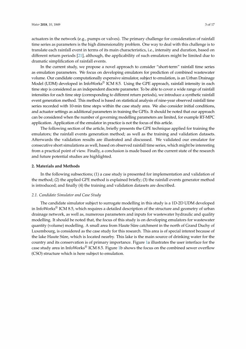
The candidate simulator subject to surrogate modelling in this study is a 1D-2D UDM developedin InfoWorks® ICM 8.5, which requires a detailed description of the structure and geometry of urbandrainage network, as well as, numerous parameters and inputs for wastewater hydraulic and qualitymodelling. It should be noted that, the focus of this study is on developing emulators for wastewaterquantity (volume) modelling. A small area from Haute Sûre catchment in the north of Grand Duchy ofLuxembourg, is considered as the case study for this research. This area is of special interest because ofthe lake Haute Sûre, which is located nearby. This lake is the main source of drinking water for thecountry and its conservation is of primary importance. Figure 1a illustrates the user interface for thecase study area in InfoWorks® ICM 8.5. Figure 1b shows the focus on the combined sewer overflow(CSO) structure which is here subject to emulation.

Water 2018, 10, 1849 4 of 17

Figure 1. (a) Case Study area in InfoWorks® ICM 8.5 interface; (b) Schematic view of combined seweroverflow (CSO) location 1.

The upstream combined wastewater flows into the main storage tank gravitationally and fromthere, it is pumped out towards the downstream of the network. The pump starts to work, on a fixedflow rate, based on a user-defined switch-on water level inside the main storage tank. In practice,the switch-on level is normally defined low enough in order to continuously convey the dry weatherflow (DWF) towards the downstream part of the network for treatment purposes in the wastewatertreatment plant (WwTP). If the wastewater level inside the main storage tank exceeds the CSO weirlevel (e.g., due to a heavy or long rainfall event), a CSO event will occur by spilling out the extrauntreated wastewater over the CSO weir to the receiving water body i.e., the lakes or rivers.

In this study, an emulator is developed to predict the short-term (daily) time series of the totalwastewater volume in CSO location 1. The total volume is the accumulated volume in the CSO tank,conduit, the main storage tank, and lastly the CSO volume, if it occurred. By predicting the totalvolume and knowing the maximum storage capacity of the CSO structure, we are able to calculate(predict) the CSO volume as a by-product of the total volume emulator.

2.2. Gaussian Process Emulator (GPE) Method

One approach to develop a dynamic GPE is, to treat the time dimension as an additional GPEtraining parameter. The main challenge in this regard is the dense coverage of the time dimension forthe output which can lead to numerical instability or computational burden [27]. However, if the focusis only on short-term predictions, this challenge is less problematic, which is the case in this study.

The surrogate modelling method used in this research is based on a GPE technique introduced inreference [28]. In this method, the model output of interest (Y) is formulated as a Gaussian processsuch that:

Y ~ N(µβ, ∑(ξy)) (1)

where µβ is a mean function which is considered linear in time, ∑ is the covariance matrix [np × np](n is the time dimension and p is the model output dimension), and ξy is the vector of covariancematrix parameters. The emulator parameters (Ψ), which are used for prediction, were determined bymaximizing the log-likelihood function (Equation (2)), introduced in reference [29], for model outputY, over a reasonable parameter range. Detailed description of the underlying mathematical frameworkof the GPE method can be found in reference [28].

lnL(Y|Ψ) =−12

(Y− µβ

)T∑−1

(Y− µβ

)− 1

2ln∣∣∑∣∣−np

2ln2π (2)

Applicability of the introduced GPE method has been approved in climate sensitivity estimationusing Markov Chain Monte Carlo (MCMC) techniques [30,31]. In the current research, we tookadvantage of this GPE method in the field of urban drainage modelling. Similar procedure can beapplied in hydrological modelling as well, when short-term predictions are of interest.

Water 2018, 10, 1849 5 of 17

An R [32] package named ‘stilt’ was used to develop the emulator in this study [33]. The GPEinputs must be prepared in the form of various simulation parameter sets with potential ranges andthe corresponding outputs can be in times series format. It should be mentioned that, for each outputof interest a separate GPE must be trained. In our research, the default optimization routine of ‘stilt’package (PORT local optimization routine) was applied to produce the results. The optimization wasimplemented twice using different initial parameter settings and the best result (maximum likelihood)selected for the emulator.

2.3. Synthetic Rainfall Generator for GPE Training

As rainfall is the main driving-force of the urban drainage system dynamics, we used observationsfrom rain gauges to quantify rainfall intensity over the studied catchment. Rain gauge measurementsare location specific, and frequently the desired information for the catchment of interest does notcorrespond to the same spatial domain where the rain gauge is located; i.e., the rain gauge canbe located outside the catchment. Even if the rain gauge is located inside the catchment (e.g.,see Figure 1a), it is important to account for the uncertainty associated to rainfall as model input basedon measurements from two additional rain gauges close-by the catchment of interest.

Commonly, model input uncertainty is characterized by defining probability distribution functions(pdfs) like those proposed in reference [34]. However, this method does not apply for the characterizationof rainfall uncertainty as model input, since rainfall time series are highly skewed due to many zeros.Therefore, it was required to apply a different approach for characterizing uncertainty in this regard.We applied the multivariate autoregressive modelling and conditional simulation approach for rainfalltime series uncertainty characterization as developed in reference [35]. This method, is suitable to simulaterainfall time series R(t) in a target catchment given known rainfall time series in two nearby locations inthe catchment RM1(t) and RM2(t), while accounting for the uncertainty that is introduced due to spatialvariation in rainfall, and the uncertainty in the measurement itself given the ratio between two nearbymeasurements. The simulation of R(t) time series is given by:

LR(t) = LRM1(t) + Lδ(t) (3)

where δ(t) is an additive factor in the log-transformation of variables, that varies over time, which iscomputed as the ratio for non-zero values between the two measured time series RM1(t) and RM2(t).The prefix L stands for the log-transformation. The method assumes that R(t), RM1(t), and δ(t) arestationary log-normally distributed stochastic processes.

Then, LRM1(t) and Lδ(t) are modelled using a multivariate autoregressive order one process [36]:[LRM1(t + 1)

Lδ(t + 1)

]=

[µRµδ

]+

[A11 A12

A21 A22

]([LRM1(t)

Lδ(t)

]−[µRµδ

])+

[εR(t + 1)εδ(t + 1)

](4)

where µR= E(LRM1); µδ = E(Lδ); A is the coefficient matrix of the autoregressive (AR) model; εR and εδare vectors of zero-mean, normally distributed white noise processes.

To calibrate this model, i.e., estimate parameters µR, µδ, A11, A12, A21, A22, σR2, σδ2, and ρRδ,where σR

2 = var(εR), σδ2 = var(εδ), and ρRδ is the correlation between εR and εδ, we derive two time

series of LRM1 and Lδ from two observed time series RM1 and RM2. Upon model calibration wesimulate from Lδ(t). This simulation should be conditional to LPo, where Po is an observed time seriesat a nearby location of RM1. Details about this conditional simulation are provided in reference [35].

We used the R-package mAr [37] to calibrate the parameters of Equation (4) given two observedtime series RM1(t) and RM2(t) to compute Lδ(t) for those non-zero values in the two time series.We present the results of calibration in Table 1.

Water 2018, 10, 1849 6 of 17

Table 1. Parameters of the synthetic rainfall generator calibrated. Vector µ, matrix A, and variance-covariancematrix C for definition of σR2, σδ

2 and ρRδ (Adapted from [35]). The presented values are casestudy specific.

Parameter Value Component Value

µR 2.8550 C11 0.0064µδ 0.1019 C33 0.0039

A11 0.9565 C13 −0.0014A12 0.0398 C12 0.0062A21 0.0243 C34 0.0034A22 0.8830 C23 −0.0014σR2 0.0724 C14 −0.0010σδ2 0.0795ρRδ −0.0388

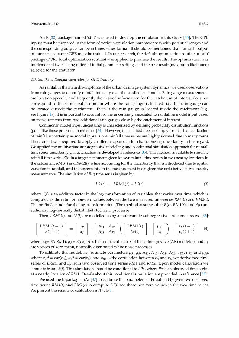
Upon calibration of the multivariate autoregressive model, we conditioned the required simulationof time series in the catchment to the observed time series Po. Figure 2 depicts the workflow forthe multivariate autoregressive modelling and conditional simulation, and event selection for therainfall generator.

Figure 2. Workflow for the multivariate autoregressive (VAR) modelling and conditional simulation(Csim), and event selection for the rainfall generator.

The workflow is based on four possible input types. The first two are the raw (in plain textformat) time series from rain gauge measurements in two different stations nearby to the study areafor calibrating the multivariate autoregressive (VAR, from vector autoregressive) model for conditionalsimulation (CSim) of the time series ensemble, which are the inputs for the event selection to composethe rainfall ensemble for training the emulator. The two stations are rain gauges from the LuxemburgishAdministration des Services Techniques de l’Agriculture (ASTA) located at Esch-sur Sûre and Dahl.The third input data can be a pre-processed time series. The pre-processing step comprises validationof the regularity of the time series, checking for no empty values, and assigning the correct time format.The fourth input data is an R object to store the location (spatial domain) of the rain gauges available.

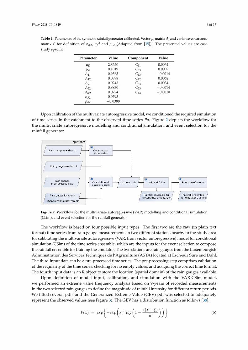
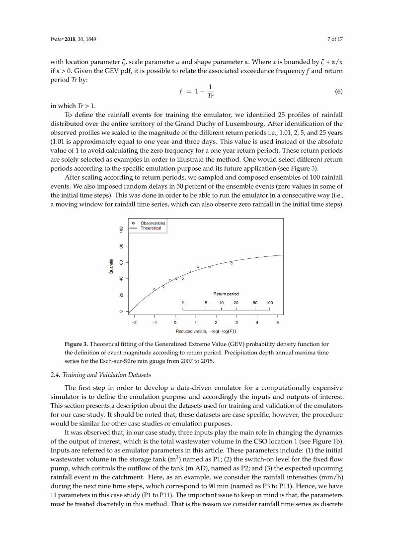
Upon definition of model input, calibration, and simulation with the VAR-CSim model,we performed an extreme value frequency analysis based on 9-years of recorded measurementsin the two selected rain gauges to define the magnitude of rainfall intensity for different return periods.We fitted several pdfs and the Generalized Extreme Value (GEV) pdf was selected to adequatelyrepresent the observed values (see Figure 3). The GEV has a distribution function as follows [38]:

F(x) = exp{−exp

(κ−1log

(1− κ(x− ξ)

α

))}(5)

Water 2018, 10, 1849 7 of 17

with location parameter ξ, scale parameter α and shape parameter κ. Where x is bounded by ξ + α/κ

if κ > 0. Given the GEV pdf, it is possible to relate the associated exceedance frequency f and returnperiod Tr by:

f = 1− 1Tr

(6)

in which Tr > 1.To define the rainfall events for training the emulator, we identified 25 profiles of rainfall

distributed over the entire territory of the Grand Duchy of Luxembourg. After identification of theobserved profiles we scaled to the magnitude of the different return periods i.e., 1.01, 2, 5, and 25 years(1.01 is approximately equal to one year and three days. This value is used instead of the absolutevalue of 1 to avoid calculating the zero frequency for a one year return period). These return periodsare solely selected as examples in order to illustrate the method. One would select different returnperiods according to the specific emulation purpose and its future application (see Figure 3).

After scaling according to return periods, we sampled and composed ensembles of 100 rainfallevents. We also imposed random delays in 50 percent of the ensemble events (zero values in some ofthe initial time steps). This was done in order to be able to run the emulator in a consecutive way (i.e.,a moving window for rainfall time series, which can also observe zero rainfall in the initial time steps).

Figure 3. Theoretical fitting of the Generalized Extreme Value (GEV) probability density function forthe definition of event magnitude according to return period. Precipitation depth annual maxima timeseries for the Esch-sur-Sûre rain gauge from 2007 to 2015.

2.4. Training and Validation Datasets

The first step in order to develop a data-driven emulator for a computationally expensivesimulator is to define the emulation purpose and accordingly the inputs and outputs of interest.This section presents a description about the datasets used for training and validation of the emulatorsfor our case study. It should be noted that, these datasets are case specific, however, the procedurewould be similar for other case studies or emulation purposes.

It was observed that, in our case study, three inputs play the main role in changing the dynamicsof the output of interest, which is the total wastewater volume in the CSO location 1 (see Figure 1b).Inputs are referred to as emulator parameters in this article. These parameters include: (1) the initialwastewater volume in the storage tank (m3) named as P1; (2) the switch-on level for the fixed flowpump, which controls the outflow of the tank (m AD), named as P2; and (3) the expected upcomingrainfall event in the catchment. Here, as an example, we consider the rainfall intensities (mm/h)during the next nine time steps, which correspond to 90 min (named as P3 to P11). Hence, we have11 parameters in this case study (P1 to P11). The important issue to keep in mind is that, the parametersmust be treated discretely in this method. That is the reason we consider rainfall time series as discrete

Water 2018, 10, 1849 8 of 17

parameters. The output of interest is the time series of the total wastewater volume for the next day(144 time steps, at 10 min resolution).

Two ensembles of 100 rainfall events with two hours duration (12 time steps with 10 minresolution) were prepared based on the method described in Section 2.3. These ensembles havesimilar summary statistics for comparability purposes; since, one of the ensembles is to producethe training dataset and the other one to make the validation dataset. Afterwards, for each dataset,2500 run scenarios are configured by various possible combinations of five samples for P1, five samplesfor P2, and 100 samples for the rainfall. Samples for P1 and P2 were selected based on minimumand maximum physical constraints in the CSO location 1. Then, these run scenarios were used assimulation input in InfoWorks® ICM 8.5 in order to build two training and validation datasets of2500 input-output pairs to train and validate the emulator. As noticed, the rainfall events consist ofthree time steps more than the rainfall parameters of the emulator, i.e., rainfall events have 12 timesteps, while we decided to have only nine time steps as emulator parameters (P3:P11). This wasdone in order to: (1) have more samples for P1, which is the initial volume in the storage tank, and;(2) neglect initial possible numerical instabilities in simulations. The same three times steps are omittedfrom output time series as well. Hence, one output time series has 141 time steps. We interfaceInfoWorks® ICM 8.5 via Ruby scripting in order to control model setup and model input, and automatethe simulations, avoiding manual ensemble simulations and data extraction. Later on, we developedan R code in order to invoke the Ruby code and have all the data generation and emulator developmentprocedure in one programming environment.

3. Results and Discussion

In this section, first, the emulator is validated using the validation dataset described earlier.Second, the effect of decreasing the training dataset size on quality of emulator is quantified and theoptimum emulator for this case study is selected accordingly. Finally, the selected emulator is usedto validate its applicability for continuous long-term simulations based on real unseen rainfall timeseries, as well as changes in initial condition and pump setting (P1 and P2).

3.1. Validation with Ensemble Validation Data

As described earlier, two separate ensemble datasets (2500 run scenarios each) with similarsummary statistics were generated by automation of InfoWorks® ICM 8.5 for training and validationpurposes. The first ensemble dataset was used to train the emulator and the second one to validatethe results produced by the emulator. Nash-Sutcliffe Efficiency (NSE) and Volumetric Efficiency(VE) were calculated as the statistics for quantification of the emulation error (Equations (7) and (8)).NSE indicates the relative magnitude of residual variance between simulation and observation [39].Whereas, VE evaluates the fraction of water delivered at the proper time (volumetric mismatch) andit can be a complementary indicator to account for the existing problems associated with NSE [40].NSE or VE equal to 1 means a perfect match between the emulator and simulator time series. The Rpackage “hydroGOF” was used to calculate these error indicators [41].

NSE = 1− ∑Ni = 1(Si −Oi)

2

∑Ni = 1

(Oi −O

)2 (7)

VE = 1− ∑Ni = 1|Si −Oi|∑N

i = 1 Oi(8)

where N is the total number of time steps; Si is the simulated value at time step i; and Oi is the observedvalue at the same time step. Here, observation refers to the results produced by the detailed simulatorand simulation is the results produced by the emulator.

Water 2018, 10, 1849 9 of 17

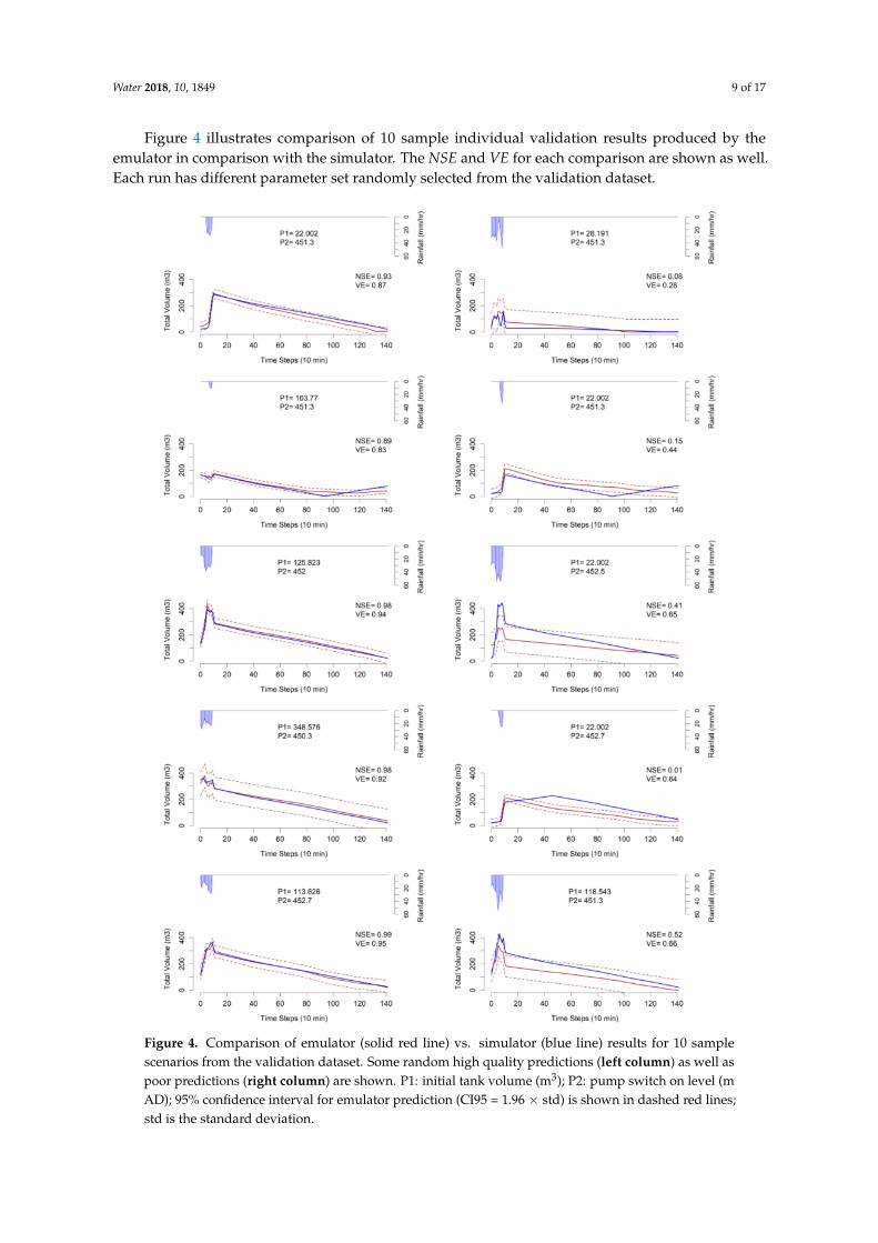
Figure 4 illustrates comparison of 10 sample individual validation results produced by theemulator in comparison with the simulator. The NSE and VE for each comparison are shown as well.Each run has different parameter set randomly selected from the validation dataset.

Figure 4. Comparison of emulator (solid red line) vs. simulator (blue line) results for 10 samplescenarios from the validation dataset. Some random high quality predictions (left column) as well aspoor predictions (right column) are shown. P1: initial tank volume (m3); P2: pump switch on level (mAD); 95% confidence interval for emulator prediction (CI95 = 1.96 × std) is shown in dashed red lines;std is the standard deviation.

Water 2018, 10, 1849 10 of 17

It should be highlighted that, the poor prediction results illustrated in Figure 4 are not as commonwithin the validation dataset and are presented for comparison purpose. Two reasons can be addressedregarding the poor predictions. First, there were only five samples for parameter P2 within the trainingdataset, while other parameters had more variations. This was due to the fact that by samplingmore values for the GPE parameters, the number of run scenarios would explode dramatically.Second, and more important, there were 11 GPE parameters in this case and we sampled from infinitepossibilities of parameter combinations for training the GPE. Hence, it is inevitable that, in some of thevalidation cases, the GPE would fail to predict the output with high accuracy since such parametercombination was not seen during the training.

In order to investigate more on the general prediction quality of the emulator, Figure 5 depicts thedistribution of emulation error indicators for all the validation dataset (2500 comparisons). Violin plotstogether with box plots of NSEs and VEs are presented in this figure. Violin plots are used to visualizethe kernel probability density of the data at different values using a mirrored density plot. A violinplot together with a box plot can be more informative regarding visualization of the distribution ofthe data. In this article, the R package “hydroGOF” [41] was used to calculate the NSE and VE values.The R package “ggplot2” [42] was applied to produce the plots accordingly.

Figure 5. Distribution of emulation error indicators Nash-Sutcliffe Efficiency (NSE) (left) andVolumetric Efficiency (VE) (right) for the validation dataset. The red square shows the mean value.Each grey dot indicates a validation run scenario.

According to Figure 5, the introduced GPE technique is capable of capturing the desired outputtime series with relatively high accuracy when compared to the original detailed simulator since, NSEand VE both are distributed towards 1 which is the best match. Besides, Q1, Q2, and Q3 quantiles ofboth distributions are located between 0.8 and 1.

At this stage, the emulator is 78 times faster than the simulator, if compared to the run time onthe same computer. It should be noted that, only hydrodynamic simulation runtime by InfoWorks®

ICM 8.5 is considered for this comparison (excluding wastewater quality modelling). This runtimeacceleration factor is obtained mainly by reducing the complexity and neglecting the numericalapproach behind the detailed simulator and fitting a model (emulator) solely based on the input andoutput data from the scenarios of the simulator runs.

It should also be mentioned that the emulator fails to predict when the inputs (parameters) are outsidethe training ranges. For instance, if the emulator is trained with rainfall intensities between 0 and 60 mm/h,it cannot be used to predict the output for an intensity of 70 mm/h. Besides, the emulator prediction resultsare worse (wider confidence interval) when there has not been sufficient training data in that range ofinputs and outputs (data insufficiency).

3.2. Selecting the Optimum Emulator

The emulator training time and runtime acceleration factor can be improved if less data is usedfor training. To achieve this the Latin Hypercube Sampling (LHS) technique [43] is used to reduce

Water 2018, 10, 1849 11 of 17

the training dataset size to 75%, 50%, 25%, 10%, 5%, and 2% of the original size. These percentageswere selected to observe the gradual effect of the dataset size reduction on emulator training timeand runtime acceleration factor. LHS is a sampling strategy based on prior information. LHS is astratified random procedure for an efficient sampling of variables from their multivariate distributions.With LHS a full coverage of the range per variable can be achieved [44]. We sampled from the outputensemble, based on the initial volume in the tank (P1). This was done to keep the parameter sets whichgenerate output time series covering the entire output space. Maximum and minimum thresholdsof the output time series are always included in the reduced ensemble. Afterwards, an emulator istrained using each dataset and validated with the same validation dataset as before (2500 scenarios).The emulation error indicators are calculated accordingly for each case. Figure 6 shows how theemulator training time decreases and runtime acceleration factor increases exponentially by reducingthe training dataset size. Figure 7 depicts the effect of reducing training dataset size on emulationerror distributions.

Figure 6. Effect of reducing the training dataset size on emulator training time (how long it takes totrain the emulator) and acceleration factor (how many times is the emulator faster than the simulator).

Figure 7. Effect of reducing the training dataset size on distribution of emulation error indicators NSE(left) and VE (right) for validation dataset (e.g., NSE075 indicates NSE distribution when 75% of thetraining data is used to train the emulator). Red square shows the mean value.

The most remarkable result to emerge from Figure 7 is that, in this case, training the emulatorwith more data does not necessarily lead to better prediction results. As it can be seen, the quality of

Water 2018, 10, 1849 12 of 17

emulator slightly improves by reducing the training dataset size to 25% or even 10% of the originaltraining dataset, and deteriorates afterwards if reduced more, although, this might not be the case ifthe output time series has a more complex and non-linear behavior. By reducing the dataset size to25% or 10%, not only the quality of emulator improves regarding emulation error indicators, but alsothe acceleration factor increases from the initial value of 78 to 380 and 1825; and emulation trainingtime decreases from the initial value of 542 min to 11.5 and 1.65 min respectively (see Figure 6).

Another important aspect to take into account while selecting the optimum emulator for thisspecific case is the confidence interval (CI) of the emulator’s predictions. Although the distributions ofNSE and VE values do not change dramatically by reducing the training dataset size, the standarddeviation of the emulator predictions (and hence CI) increase in the same time (wider CIs) due to lesstraining data. Hence, it is advised to consider the emulator trained by 25% of the data as the optimumemulator in this case. This emulator is 380 times faster than the simulator.

3.3. Leave-One-Out Cross-Validation Analysis

So far, the emulation error indicators (NSE and VE) were calculated based on comparisonof emulator and simulator results at all the time steps within the output time series (24 h).However, in some applications, one would be more interested in having high emulation accuracy atsome specific time steps. Hence, in this step the optimum emulator is tested based on leave-one-outcross-validation analysis in order to investigate the prediction quality in specific time steps.

In this method, first, each individual run in the training ensemble is excluded from the emulator,and then the emulator is used to predict the output based on the excluded parameter set. This processis repeated for each individual run in the training ensemble and for each trial the emulator predictionvs. the actual simulator output is plotted and the normalized prediction error is calculated accordingly,as the percentage of the total range of the output. A perfect match between the emulator and simulatorresults must be exactly located on a 1:1 line [33].

Figure 8 summarizes the leave-one-out cross-validation analysis results for the selected optimumemulator. The analyses are performed for sample specific time steps at the beginning (TS = 7), middle(TS = 70) and the end (TS = 140) of the output time series. This is done to investigate more precisely theemulator’s prediction quality. One would select different time steps based on specific emulation purposes.

Figure 8. Cont.

Water 2018, 10, 1849 13 of 17

Figure 8. Leave-one-out cross-validation analysis results for time steps 7, 70, and 140 (a–c respectively).

As it can be observed here, the emulator quality is considerably high at the beginning of theprediction time series (TS = 7). On the contrary, the prediction quality deteriorates gradually if wemove towards TS = 70 or 140. This behavior is directly related to the training data used to developthe emulator. First of all, the density of the training output ensemble is higher within the initial timesteps and more scattered towards the end of the output time series. Second, the effect of the majorityof the training parameters, including the initial volume (P1) and the rainfall scenario (P3:P11), is morerelevant at the beginning of the prediction time series.

The middle and end of the prediction time series is mainly affected by P2, which is the switch-onlevel for the operating pump to deplete the storage tank. As mentioned earlier in Section 2.4, onlyfive samples for P2 are considered in the training dataset. One would include more samples for P2 toimprove the prediction quality at the end of the output time series. However, by increasing the numberof the samples for P2, the number of ensembles in the training dataset will increase dramatically.For instance, adding only two more samples for P2, will lead to one thousand more scenarios in thetraining ensemble (5 × 7 × 100 = 3500) and hence longer training time for the emulator; although,in that case the LHS can be used again to reduce the training dataset size.

The current emulator would be interesting in applications such as RT-MPC in which the qualityof the few initial time steps of the prediction is much more important, in comparison with the finaltime steps of the prediction horizon.

3.4. Validation for CSO Events Prediction

In this section, the selected emulator from the previous step (trained by 25% of the training dataset)is used to validate the applicability of the emulator regarding CSO events prediction. As mentionedearlier, it is possible to predict the potential CSO event as a by-product of the total volume emulation.To do so, it is only required to subtract the maximum storage capacity at the CSO location from thetotal predicted volume by the emulator.

Around 66% of the scenarios in the validation dataset (2500 scenarios) result in CSO events. It wasobserved that, the emulator is able to predict occurrence of CSO events in 82% of these cases. In 3%of the scenarios false alarm was observed (i.e., prediction of CSO event while there is no such event).Figure 9 compares the distributions of error indicators NSE and VE, for CSO predictions vs. the totalvolume predictions, using the emulator.

Water 2018, 10, 1849 14 of 17

Figure 9. Comparison between distributions of emulation error indicators NSE (left) and VE (right)for CSO predictions vs. total volume predictions. Red square shows the mean value.

Although the emulator is able to predict occurrence of CSO events in 82% of the cases; Figure 9shows that, for the CSO event prediction, the NSE and VE distributions are not as satisfactory asthe total volume emulation. The deterioration of the results is more visible regarding the volumetricefficiency (VE) which is in fact a more important error indicator for CSO volume prediction. The mainreason for this behavior is that the emulator was trained solely based on the data regarding the totalvolume and not the CSO volume. CSO volume is calculated as a side-product of the total volume.Hence, the quality of CSO prediction is worse than total volume prediction.

These CSO prediction results are still valuable regarding applications such as RTC, in whichavoidance of CSO event “occurrence” is the priority, regardless of the precise CSO volume prediction.For instance, normally, in CSO management regulations for different countries, there is a limitation forthe “number” of allowed CSO events per year according to the receiving water bodies [45], rather thantheir precise volume.

3.5. Validation for Applicability in Real Consecutive Scenarios

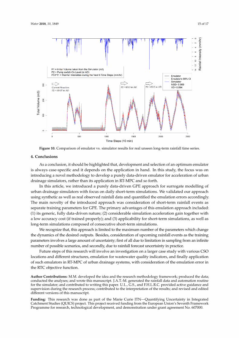
As mentioned repeatedly earlier, the purpose of introducing the GPE technique in this study is itsapplication for short-term simulations. Such simulations are favorable in applications such as ModelPredictive Control (MPC) for RTC purpose. In MPC, frequent, numerous, and continuous short-termsimulations are implemented in each time step for optimization of the control actions in the predictionhorizon. Therefore, in this section, we validate our emulator for continuous repetitive short-termsimulations with real observed rainfall time series in the case study catchment. In each nine timesteps, the emulator obtains the initial volume from the simulator time series (P1), the pump-on level(P2) which can be a control action in MPC setup, and the upcoming real rainfall scenario for the next90 min (P3:P11). Then based on these parameters (P1:P11) the emulator can predict the total volumeaccordingly for the next day. The nine initial time steps are aggregated and plotted in Figure 10.

Figure 10 indicates the applicability of the introduced GPE emulator for a long-term simulation(2476 time steps, around 17 days) which is composed of numerous consecutive short-term simulations,with altering the GPE parameters in between simulations. P2 is altered twice within the long timeseries to show the possibility of increasing the pump switch-one level in order to store more wastewater in the retention tank if needed. Although, there are few cases in which the deviation betweenemulator and simulator is beyond the 95% confidence interval, the overall simulator time seriesis within the confidence interval of the emulator with a considerably high overall emulation errorindicators (NSE = 0.969 and VE = 0.894).

Water 2018, 10, 1849 15 of 17

Figure 10. Comparison of emulator vs. simulator results for real unseen long-term rainfall time series.

4. Conclusions

As a conclusion, it should be highlighted that, development and selection of an optimum emulatoris always case-specific and it depends on the application in hand. In this study, the focus was onintroducing a novel methodology to develop a purely data-driven emulator for acceleration of urbandrainage simulators, rather than its application in RT-MPC and so forth.

In this article, we introduced a purely data-driven GPE approach for surrogate modelling ofurban drainage simulators with focus on daily short-term simulations. We validated our approachusing synthetic as well as real observed rainfall data and quantified the emulation errors accordingly.The main novelty of the introduced approach was consideration of short-term rainfall events asseparate training parameters for GPE. The primary advantages of this emulation approach included:(1) its generic, fully data-driven nature; (2) considerable simulation acceleration gain together witha low accuracy cost (if trained properly); and (3) applicability for short-term simulations, as well aslong-term simulations composed of consecutive short-term simulations.

We recognize that, this approach is limited to the maximum number of the parameters which changethe dynamics of the desired outputs. Besides, consideration of upcoming rainfall events as the trainingparameters involves a large amount of uncertainty; first of all due to limitation in sampling from an infinitenumber of possible scenarios, and secondly, due to rainfall forecast uncertainty in practice.

Future steps of this research will involve an investigation on a larger case study with various CSOlocations and different structures, emulation for wastewater quality indicators, and finally applicationof such emulators in RT-MPC of urban drainage systems, with consideration of the emulation error inthe RTC objective function.

Author Contributions: M.M. developed the idea and the research methodology framework; produced the data;conducted the analyses; and wrote this manuscript. J.A.T.-M. generated the rainfall data and automation routinefor the simulator; and contributed to writing this paper. U.L., G.S., and F.H.L.R.C. provided active guidance andsupervision during the research process; contributed to the interpretation of the results; and revised and editeddifferent versions of this manuscript.

Funding: This research was done as part of the Marie Curie ITN—Quantifying Uncertainty in IntegratedCatchment Studies (QUICS) project. This project received funding from the European Union’s Seventh FrameworkProgramme for research, technological development, and demonstration under grant agreement No. 607000.

Water 2018, 10, 1849 16 of 17

Acknowledgments: The authors also thank the Luxemburgish Administration des Services Techniques del’Agriculture (ASTA) for the rainfall time series, as well as the Observatory for Climate and Environment (OCE) inLIST for the technical support.

Conflicts of Interest: The authors declare no conflict of interest. The founding sponsors had no role in the designof the study; in the collection, analyses, or interpretation of data; in the writing of the manuscript, and in thedecision to publish the results. All authors copy-edited this manuscript.

References

1. Asher, M.J.; Croke, B.F.W.; Jakeman, A.J.; Peeters, L.J.M. A review of surrogate models and their applicationto groundwater modeling. Water Resour. Res. 2015, 51, 5957–5973. [CrossRef]

2. Galelli, S.; Castelletti, A.; Geodbleod, A. High-Performance Integrated Control of water quality and quantityin urban water reservoirs. Water Resour. Res. 2015, 4840–4847. [CrossRef]

3. Machac, D.; Reichert, P.; Albert, C. Emulation of dynamic simulators with application to hydrology.J. Comput. Phys. 2016, 313, 352–366. [CrossRef]

4. Dipierro, F.; Khu, S.; Savic, D.; Berardi, L. Efficient multi-objective optimal design of water distribution networkson a budget of simulations using hybrid algorithms. Environ. Model. Softw. 2009, 24, 202–213. [CrossRef]

5. Stone, N. Gaussian Process Emulators for Uncertainty Analysis in Groundwater Flow. Ph.D. Thesis,The University of Nottingham, Nottingham, UK, 2011.

6. Fraga, I.; Cea, L.; Puertas, J.; Suarez, J.; Jimenez, V.; Jacome, A. Global Sensitivity and GLUE-BasedUncertainty Analysis of a 2D-1D Dual Urban Drainage Model. J. Hydrol. Eng. 2016, 21, 1–11. [CrossRef]

7. O’Hagan, A. Bayesian analysis of computer code outputs: A tutorial. Reliab. Eng. Syst. Saf. 2006, 91,1290–1300. [CrossRef]

8. Blanning, R.V. The construction and implementation of metamodels. Simulation 1975, 24, 177–184. [CrossRef]9. Willcox, K.E.; Peraire, J. Balanced model reduction via the proper orthogonal decomposition. AIAA J. 2002,

40, 2323–2330. [CrossRef]10. Bieker, H.P.; Al, E. Real-time production optimization of oil and gas production systems: A technology

survey. SPE Prod. Oper. 2007, 22, 382–391. [CrossRef]11. Robinson, T.; Eldred, M.; Willcox, K.; Haimes, R. Surrogate-based optimization using multifidelity models

with variable parameterization and corrected space mapping. AIAA J. 2008, 46, 2814–2822. [CrossRef]12. Regis, R.G.; Shoemaker, C.A. Constrained global optimization of expensive black box functions using radial

basis functions. J. Glob. Opt. 2005, 31, 153–171. [CrossRef]13. Razavi, S.; Tolson, B.A.; Burn, D.H. Review of surrogate modeling in water resources. Water Resour. Res.

2012, 48. [CrossRef]14. Mahmoodian, M. Concept and Methodologies to Guide Surrogate Modelling for Real-Time Control (RTC) of

Urban Drainage Systems under Uncertainty; EU ITN Project Report; QUICS: Belvaux, Luxembourg, 2018.Available online: https://www.sheffield.ac.uk/quics/dissemination/reports (accessed on 23 April 2018).

15. Mahmoodian, M.; Carbajal, J.P.; Bellos, V.; Leopold, U.; Schutz, G.; Clemens, F. A Hybrid Surrogate ModellingStrategy for Simplification of Detailed Urban Drainage Simulators. Water Resour. Manag. 2018, 27. [CrossRef]

16. Zhang, Q.; Stanley, J.S. Real-time water treatment process control with artificial neural networks.J. Environ. Eng. 2000, 125, 124–137.

17. Soltani, F.; Kerachian, R.; Shirangi, E. Developing operating rules for reservoirs considering the water qualityissues: Application of ANFIS-based surrogate models. Expert Syst. Appl. 2010, 37, 6639–6645. [CrossRef]

18. Wu, Z.Y.; El-Maghraby, M.; Pathak, S. Applications of deep learning for smart water networks. In 13thComputer Control for Water Industry Conference, CCWI 2015 Applications; Elsevier B.V.: New York, NY, USA,2015; Volume 119, pp. 479–485.

19. Han, H.-G.; Qiao, J.-F.; Chen, Q.-L. Model predictive control of dissolved oxygen concentration based on aself-organizing RBF neural network. Control Eng. Pract. 2012, 20, 465–476. [CrossRef]

20. Moreno-Rodenas, A.M.; Bellos, V.; Langeveld, J.G.; Clemens, F.H.L.R. A dynamic emulator for physically basedflow simulators under varying rainfall and parametric conditions. Water Res. 2018, 142, 512–527. [CrossRef]

21. Carbajal, J.P.; Leitão, J.P.; Albert, C. Appraisal of data-driven and mechanistic emulators of nonlinearhydrodynamic urban drainage simulators. arXiv, 2016; arXiv:1609.08395v1.

22. MUCM Community. Managing Uncertainty in Complex Models, MUCM Toolkit. Available online:http://www.mucm.ac.uk/ (accessed on 8 February 2017).

Water 2018, 10, 1849 17 of 17

23. Castelletti, A.; Galelli, S.; Restelli, M.; Soncini-Sessa, R. Data-driven dynamic emulation modelling for theoptimal management of environmental systems. Environ. Model. Softw. 2011, 34, 30–43. [CrossRef]

24. Castelletti, A.; Galelli, S.; Ratto, M.; Soncini-Sessa, R.; Young, P.C. A general framework for DynamicEmulation Modelling in environmental problems. Environ. Model. Softw. 2012, 34, 5–18. [CrossRef]

25. Machac, D.; Reichert, P.; Rieckermann, J.; Albert, C. Fast mechanism-based emulator of a slow urbanhydrodynamic drainage simulator. Environ. Model. Softw. 2016, 78, 54–67. [CrossRef]

26. Gladish, D.W.; Pagendam, D.E.; Peeters, L.J.M.; Kuhnert, P.M.; Vaze, J. Emulation Engines: Choice andQuantification of Uncertainty for Complex Hydrological Models. J. Agric. Biol. Environ. Stat. 2017, 23, 39–62.[CrossRef]

27. Reichert, P.; White, G.; Bayarri, M.J.; Pitman, E.B. Mechanism-based emulation of dynamic simulationmodels: Concept and application in hydrology. Comput. Stat. Data Anal. 2011, 55, 1638–1655. [CrossRef]

28. Olson, R.; Chang, W. Mathematical Framework for a Separable Gaussian Process Emulator; PennState College ofEarth and Mineral Sciences: University Park, PA, USA, 2013.

29. Rasmussen, C.E.; Williams, C.K.I. Gaussian Processes for Machine Learning; MIT Press: Cambridge, MA, USA, 2006.30. Olson, R.; Sriver, R.; Goes, M.; Urban, N.M.; Matthews, H.D.; Haran, M.; Keller, K. A climate sensitivity

estimate using Bayesian fusion of instrumental observations and an Earth System model. J. Geophys.Res. Atmos. 2012, 117, 1–11. [CrossRef]

31. Olson, R.; Sriver, R.; Chang, W.; Haran, M.; Urban, N.M.; Keller, K. What is the effect of unresolved internalclimate variability on climate sensitivity estimates? J. Geophys. Res. Atmos. 2013, 118, 4348–4358. [CrossRef]

32. R Foundation for Statistical Computing. R: A Language and Environment for Statistical Computing; R Foundationfor Statistical Computing: Vienna, Austria, 2014.

33. Olson, R.; Chang, W.; Keller, K.; Haran, M.R. Package ‘stilt.’ CRAN. Available online: https://cran.r-project.org/(accessed on 15 August 2018).

34. Heuvelink, G.B.M.; Brown, J.D.; Brown, E.E. A probabilistic framework for representing and simulatinguncertain environmental variables. Int. J. Geogr. Inf. Sci. 2007, 21, 497. [CrossRef]

35. Torres-Matallana, J.A.; Leopold, U.; Heuvelink, G.B.M. Multivariate autoregressive modelling andconditional simulation of precipitation time series for urban water models. Eur. Water 2017, 57, 299–306.

36. Luetkepohl, H. New Introduction to Multiple Time Series Analysis; Springer: Berlin/Heidelberg, Germany, 2005.37. Barbosa, S.M. mAr: Multivariate AutoRegressive Analysis, R package version 1.1-2.; R Foundation for Statistical

Computing: Vienna, Austria, 2012.38. Hosking, J.R.M. L-Moments: Analysis and Estimation of Distributions Using Linear Combinations of Order

Statistics. J. R. Stat. Soc. Ser. 1990, 52, 105–124. [CrossRef]39. Nash, J.E.; Sutcliffe, I.V. River flow forecasting throligh conceptual models part i—A disclission of principles.

J. Hydrol. 1970, 10, 282–290. [CrossRef]40. Criss, R.E.; Winston, W.E. Do Nash values have value? Discussion and alternate proposals. Hydrol. Processes

2008, 22, 2723–2725. [CrossRef]41. Zambrano-Bigiarini, M. R Package ‘hydroGOF’. Available online: https://cran.r-project.org/ (accessed on

8 August 2017).42. Wickham, H. Ggplot2: Elegant Graphics for Data Analysis. Available online: https://cran.r-project.org/

(accessed on 25 October 2018).43. Roudier, P. R Package ‘clhs’—Conditioned Latin Hypercube Sampling. Available online: https://cran.r-

project.org/ (accessed on 10 October 2018).44. Minasny, B.; McBratney, A.B. A conditioned Latin hypercube method for sampling in the presence of ancillary

information. Comput. Geosci. 2006, 32, 1378–1388. [CrossRef]45. Toffol, S. De Sewer System Performance Assessment—An Indicators Based Methodology; Universität Innsbruck:

Innsbruck, Austria, 2006.

© 2018 by the authors. Licensee MDPI, Basel, Switzerland. This article is an open accessarticle distributed under the terms and conditions of the Creative Commons Attribution(CC BY) license (http://creativecommons.org/licenses/by/4.0/).