Delft University of Technology Precision Constrained...

Delft University of Technology

Precision Constrained Optimization by Exponential Ranking

Bittermann, Michael; Ciftcioglu, Ozer

DOI10.1109/CEC.2016.7744072Publication date2016Document VersionPeer reviewed versionPublished inProceedings 2016 IEEE Congress on Evolutionary Computation (CEC)

Citation (APA)Bittermann, M., & Ciftcioglu, O. (2016). Precision Constrained Optimization by Exponential Ranking. InProceedings 2016 IEEE Congress on Evolutionary Computation (CEC) (pp. 2296-2305). IEEE. DOI:10.1109/CEC.2016.7744072

Important noteTo cite this publication, please use the final published version (if applicable).Please check the document version above.

CopyrightOther than for strictly personal use, it is not permitted to download, forward or distribute the text or part of it, without the consentof the author(s) and/or copyright holder(s), unless the work is under an open content license such as Creative Commons.

Takedown policyPlease contact us and provide details if you believe this document breaches copyrights.We will remove access to the work immediately and investigate your claim.

This work is downloaded from Delft University of Technology.For technical reasons the number of authors shown on this cover page is limited to a maximum of 10.

http://dx.doi.org/10.1109/CEC.2016.7744072

Precision Constrained Optimization by Exponential Ranking

Michael S. Bittermann

Department of Architecture Maltepe University

Istanbul, Turkey [email protected]

Özer Ciftcioglu, Senior Member, IEEE Department of Architecture

Delft University of Technology, Delft, The Netherlands Maltepe University, Istanbul, Turkey

[email protected] [email protected]

Abstract—Demonstrative results of a probabilistic constraint handling approach that is exclusively using evolutionary computation are presented. In contrast to other works involving the same probabilistic considerations, in this study local search has been omitted, in order to assess the necessity of this deterministic local search procedure in connection with the evolutionary one. The precision stems from the non-linear probabilistic distance measure that maintains stable evolutionary selection pressure towards the feasible region throughout the search, up to micro level in the range of 10-10 or beyond. The details of the theory are revealed in another paper [1]. In this paper the implementation results are presented, where the non-linear distance measure is used in the ranking of the solutions for effective tournament selection. The test problems used are selected from the existing literature. The evolutionary implementation without local search turns out to be already competitively accurate with sophisticated and accurate state-of-the-art constrained optimization algorithms. This indicates the potential for enhancement of the sophisticated algorithms, as to their precision and accuracy, by the integration of the proposed approach.

Keywords—evolutionary algorithm; multiobjective optimization; constrained optimization; probabilistic modeling

I. INTRODUCTION

Evolutionary algorithms have become the most prominent approach for solving optimization problems during the three decades of their emergence. The advancements have been surprisingly rapid, presumably due to the simplicity of the original concept and its broad applicability that includes situations where insight into a problem is minimal. Today the evolutionary computation literature encompasses many advanced optimization algorithms having the spirit of genetic algorithms in essence. Updated surveys are reported in the literature from time to time, e.g. [2, 3]. The development process of the methodology may be broadly categorized as follows. The hallmarks of the first half are the developments along single objective optimization, and those of the second half were multiobjective optimizations in Pareto sense. As to the latter there are a number of excellent text books contributing to the advancement of evolutionary multiobjective optimization [4-6]. During both periods the main focus was on solving unconstrained problems; however, within each period, gradually more and more attention was paid to constrained optimization. Since multiobjective optimization

can be formulated as a single objective with constraints, where the constraints are the rest of the objectives subject to minimization, constrained optimization with a single objective function in some sense is a general case, and this is the case in this work. A widely used method for constrained optimization is the penalty function method. Penalty function method penalizes a solution, which deteriorates the fitness of a solution when it violates constraints. This penalization is accomplished by adding a value to the objective function value in proportion to the amount of constraint violation, where the proportionality factor is known as the penalty parameter. A strategy that did not require a penalty parameter in evolutionary constrained optimization was proposed by Deb in 2000 [7], which is superseded by another research with the penalty parameter [8]. In this approach during the tournament selection process an infeasible solution is always treated as inferior compared to a feasible one, or as inferior to a solution that violates the constraints to a lesser extent. Coello [9] proposed a self-adaptive penalty approach by using a co-evolutionary model to adapt the penalty factors. However, in general determination of a right penalty parameter still remained an issue.

Within the methodological framework of the penalty parameter approach, local search in combination with evolutionary computation (EC) has shown to be effective for solving constrained optimization problems [8]. In this combination the local search is an alternative for selection pressure in precision demanding problems. The role of EC in the joint evolutionary-classical approach is not the search for a feasible solution, but to produce a suitable starting condition for the effective execution of the local search, so that the actual reaching of feasible solution is essentially due to the local search and not due to the evolutionary computation. In an earlier study the effectiveness of local-search based evolutionary constrained optimization was enhanced by introducing a probabilistic distance metric into the evolutionary component of the method [10]. From the mentioned joint-evolutionary works, as their effectiveness is essentially due to local search, one can get the impression that a deterministic procedure, such as local search, is rather imperative in order to enable EC for constrained optimization.

Proc. IEEE World Congress on Computational Intelligence - WCCI 2016, 24-29 July, Vancouver, Canada

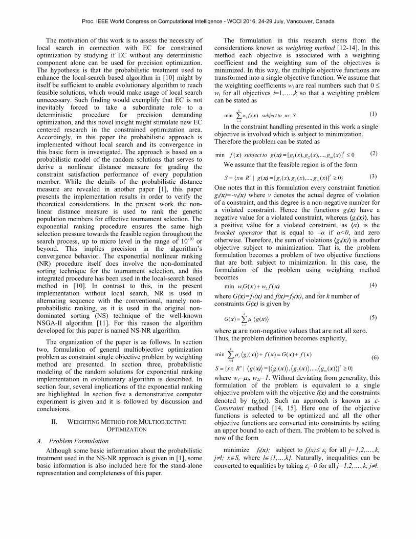
The motivation of this work is to assess the necessity of local search in connection with EC for constrained optimization by studying if EC without any deterministic component alone can be used for precision optimization. The hypothesis is that the probabilistic treatment used to enhance the local-search based algorithm in [10] might by itself be sufficient to enable evolutionary algorithm to reach feasible solutions, which would make usage of local search unnecessary. Such finding would exemplify that EC is not inevitably forced to take a subordinate role to a deterministic procedure for precision demanding optimization, and this novel insight might stimulate new EC centered research in the constrained optimization area. Accordingly, in this paper the probabilistic approach is implemented without local search and its convergence in this basic form is investigated. The approach is based on a probabilistic model of the random solutions that serves to derive a nonlinear distance measure for grading the constraint satisfaction performance of every population member. While the details of the probabilistic distance measure are revealed in another paper [1], this paper presents the implementation results in order to verify the theoretical considerations. In the present work the non-linear distance measure is used to rank the genetic population members for effective tournament selection. The exponential ranking procedure ensures the same high selection pressure towards the feasible region throughout the search process, up to micro level in the range of 10-10 or beyond. This implies precision in the algorithm’s convergence behavior. The exponential nonlinear ranking (NR) procedure itself does involve the non-dominated sorting technique for the tournament selection, and this integrated procedure has been used in the local-search based method in [10]. In contrast to this, in the present implementation without local search, NR is used in alternating sequence with the conventional, namely non-probabilistic ranking, as it is used in the original non- dominated sorting (NS) technique of the well-known NSGA-II algorithm [11]. For this reason the algorithm developed for this paper is named NS-NR algorithm.

The organization of the paper is as follows. In section two, formulation of general multiobjective optimization problem as constraint single objective problem by weighting method are presented. In section three, probabilistic modeling of the random solutions for exponential ranking implementation in evolutionary algorithm is described. In section four, several implications of the exponential ranking are highlighted. In section five a demonstrative computer experiment is given and it is followed by discussion and conclusions.

II. WEIGHTING METHOD FOR MULTIOBJECTIVE OPTIMIZATION

A. Problem Formulation

Although some basic information about the probabilistic treatment used in the NS-NR approach is given in [1], some basic information is also included here for the stand-alone representation and completeness of this paper.

The formulation in this research stems from the considerations known as weighting method [12-14]. In this method each objective is associated with a weighting coefficient and the weighting sum of the objectives is minimized. In this way, the multiple objective functions are transformed into a single objective function. We assume that the weighting coefficients wi are real numbers such that 0 wi for all objectives i=1,….,k so that a weighting problem

can be stated as

1

min ( )k

i ii

w f subject to S

x x (1)

In the constraint handling presented in this work a single objective is involved which is subject to minimization. Therefore the problem can be stated as

1 2min ( ) ( [ ( ), ( ),..., ( )] 0Tmf subject to g g x g x g x x x) = (2)

We assume that the feasible region is of the form

1 2{ | ( [ ( ), ( ),..., ( )] 0}n TmS x R g g x g x g x x) = (3)

One notes that in this formulation every constraint function gi(x)=-vi(x) where v denotes the actual degree of violation of a constraint, and this degree is a non-negative number for a violated constraint. Hence the functions gi(x) have a negative value for a violated constraint, whereas gi(x) , has a positive value for a violated constraint, as α is the bracket operator that is equal to –α if α<0, and zero otherwise. Therefore, the sum of violations gi(x) is another objective subject to minimization. That is, the problem formulation becomes a problem of two objective functions that are both subject to minimization. In this case, the formulation of the problem using weighting method becomes

1 2min ( ) (w G w fx x) (4)

where G(x)=f1(x) and f(x)=f2(x), and for k number of constraints G(x) is given by

1

( ) ( )k

ii

G g

x x (5)

where μarenon‐negativevaluesthatarenotallzero. Thus, the problem definition becomes explicitly,

1

1 2

min ( ) ( ) ( ) ( )

{ | ( [ ( ) , ( ) ,..., ( ) ] 0}

k

i ii

n Tm

g f G f

S x R g g g g

x x x x

x) = x x x

(6)

where w1=i, w2i=1. Without deviating from generality, this formulation of the problem is equivalent to a single objective problem with the objective f(x) and the constraints denoted by gj(x) . Such an approach is known as -Constraint method [14, 15]. Here one of the objective functions is selected to be optimized and all the other objective functions are converted into constraints by setting an upper bound to each of them. The problem to be solved is now of the form

minimize fl(x); subject to fj(x) j for all j=1,2,….,k, jl; xS, where l{1,…,k}. Naturally, inequalities can be converted to equalities by taking j=0 for all j=1,2,….,k, jl.


B. Issues of the penalty function approach

Conventionally, (6) is written in the form

1

min ( , ) ( ) ( )J

j jj

P R f R g

x x x (7)

where function gj(x) is considered to be a penalty function and the parameters Rj are the associated penalty parameters; Since each individual Rj is not known, conventionally a common penalty parameter R is defined so that (7) becomes

1

min ( , ) ( ) ( )J

jj

P R f R g

x x x (8)

or taking f2(x) =f(x) and the summation of the gj(x) functions as f1(x), we can write

2 1min{ ( ) ( )}optP f R f x x (9)

To solve the optimization problem given by (9) with the weighting method, one can consider some options as follows.

Approach to the final optimal solution by means of constant Fig. 1.

penalty parameter R.

a) R is a constant. In this case, the development of the optimal front is illustrated in figure 1. The final development is the theoretical front and the solution is denoted with the point T which is far from the optimal point denoted by Popt. As result of this option some gradient-based search algorithm is necessary that tails up evolutionary computation to reach the optimal point if it is realizable at all due to the chance of getting trapped in some local optima. During the Pareto front formation the most of the attention of the chromosomes goes to the penalty function rather than the objective function. As result of this, the convergence is essentially due to the constraints and therefore there is a significant progress along that line, while the single objective is de facto subsumed under the constraints. This situation makes determination of R very critical and precarious at the same time.

b) To determine the penalty parameter with adaptation by means of an extrapolation polynomial. In this case, a polynomial is fitted to the optimal front and its extrapolated intersection with the objective function axis is used for the slope of the tangent which is the reasonable estimation of the penalty parameter R. However, in this case, search algorithm tends to move to the straightforward solution, which is the gradual diminishing of the slope as illustrated in figure 2. As result of this option the penalty parameter takes smaller values during the search and may eventually vanish. In

the extreme, R goes to zero and problem turns out to be a single objective optimization omitting the constraints.

Approach to the final optimal solution by means of penalty Fig. 2. function approach, where R is the penalty parameter being

estimated through curve fitting

C. Analysis of penalty function parameter

Let us assume that optimal theoretical front compromises the solutions for the objectives f1(x) and f2(x), where objective f1(x) admits to be minimally zero. For the analysis viewpoint we assume that Pareto front is symmetrical with respect to f1(x) and f2(x), and the front is an envelope of a line crossing the f1(x) axis at the point t and crossing the f2(x) axis at the point Popt-t; t is a parameter related to parametric representation of a line tangent to the Pareto front, and it is represented by

2 1( ) ( )1

opt

f f

t P t

x x (10)

In (10), Popt is the optimum solution, where f2(x )=Popt =t and f1(x ) =0, which represents the satisfaction of the constraint. From (10), we obtain

2 1( ) ( )( )opt

tf f t

t P

x x

x (11)

We can define the slope

( )opt

tr

t P

x (12)

as a kernel penalty parameter representing the varying part

The envelope of tangent and the new penalty parameter r Fig. 3.

of the general penalty parameter R in (8), and for each constraint we consider r=rj . The envelope of the tangent in (10) is shown in figure 3. In words, r is the gain in f2(x) per unit decrease in f1(x) at the point of tangent F and within infinitesimally small interval of f1(x). Incidentally, the envelope of the tangent is determined by the following condition [1]

2 2 1( ) ( ) ( )t f x f x f x (13)


And substitution of (13) in (11) yields the Pareto front expression as

22 1 1 2[ ( ) ( )] 2[ ( ) ( )] 0optf x f x f x f x P (14)

Variation of r during the minimization process for a given constraint j is shown in figure 4.

Nondominated Sorting-Nonlinear Ranking (NS-NR) approach to Fig. 4.

the final optimal solution by means of penalty function approach; r is the penalty parameter.

As shown in the figure, as the process approaches to the minimum, the slope tends to approach infinity. Therefore, in this work penalty parameter R in (7) is not a constant, but it is a varying parameter, adapted during the search process, which is peculiar to this work.

The kernel penalty parameter r is zero for t=0 and it monotonically increases as t increases, as seen in (12), and t is given by (13). As Popt is reached, at this point f2(x)=0, and t=f2(x) where t=Popt. For t=Popt the kernel penalty parameter r goes to infinity, as seen in (11). Alternatively, this work shows that the kernel parameter r is a function of the objective functions f1 and f2, and at the end of the search process the intersection of the tangent given by (10) is the minimum being sought for, where f1=0 and f2 is the minimum. At that point Pareto front and tangent disappear, and they reduce to the point Popt. A convergence approach complying with (12) exhibits two gains:

Approach to optimum is systematic and therefore robust without precarious tangent slope computations

No local search for Popt is necessary.

Implementation of the approach is due to a probabilistic modeling of the random solutions in the evolutionary computation and ensuing nonlinear ranking. These are presented in the following section

III. PROBABILISTIC MODELING FOR EXPONENTIAL RANKING

Referring to (6), in a general constrained optimization problem the problem formulation is written as

1

min ( ) ( ) ( )J

j jj

P f g

x x x (15)

where f(x) is the single objective function to be minimized; gj(x) is the violation of the gi-th constraint, namely penalty

function, µi is the associated parameter of the penalty function. Since gj(x) is at each generation continually tried to be vanishing during the evolutionary minimization

process, considering the population density of solutions, the probability density of gj(x) is highest about zero violations, and its value gradually diminishes proportional with the degree of violation. Based on the randomly generated population of the evolutionary algorithm, we can model the violations as a random variable, where the violations are independent due to random population formation by the random composition of chromosomes at each generation. The number of violations per unit violation gradually decreases with the degree of violation conforming to the commensurate number of chromosomes created by the elitism and sorting strategy in the genetic algorithm. This probabilistic pattern continues in the same way without change throughout the generations. The probabilistic description of this process can be modeled by the exponential probability density (pdf), because of its memorylessness property. That is the form of the density remains the same being independent of the range it models, while the exponential pdf is a unique density having this property. With this information peculiar to the subject matter of this research, we can confidently apply the exponential pdf, which is given by

( ) yf y e (16)

where is the decay parameter. Denoting

( )jy g x (17)

the pdf in (16) becomes

( ) j j

j

g

j jgf g e

(18)

The mean value of the exponential pdf function is equal to j

-1. During the evolutionary search gj(x) is a general form of violation which applies to any member s of the population although s is not explicitly denoted. However, in explicit form, we can write

,

,( ) j j s

j

g

j s jgf g e

(19)

where s denotes a population member. We can characterize the exponential pdf function according to the constraint j simply by equating the mean value of the violations gj to the mean of the exponential pdf, namely

1/j jg

(20)

One should note that the mean of the exponential probability density of gj is equivalent to the mean of a uniform probability density applied to the violations gj . Therefore the mean of the exponential density function is estimated by taking the mean of the violations which are from a uniform probability density and they are independent.

Since a violation gj spans all the violations starting from zero up to the point gj , the probability of the violation is expressed as cumulative distribution function whose implication is easy to comprehend by considering the extremes. The cumulative distribution function of (16) is given by


0

1( ) 1

j j

j j j

g g

g g g

j j

j

p g e dg eg

(21)

For gj =0 violation is zero and for gj =, violation is 1, i.e., 100% for a finite mean value of gj(x) . Explicitly p( gj ) is the probability of a violation in the range between zero and gj . It is a monotonically increasing function complying with the boundary conditions of gj(x) which varies between zero and infinity. It is interesting to note that for zero constraint violation the exponential probability density is at its maximum and probability of violation at its minimum. The probability p( gj ) is an appropriate measure for the magnitude or effectiveness of a violation, and it can be considered as a probabilistic distance function or a metric measuring the distance from the zero violation, fulfilling all the conditions to be a distance measure [16, 17]. The important implication of the premise (21) will be seen shortly.

The optimization problem with constraints is formulated in this work as follows.

1

( ) ( ) ) ( )J

j j j jj

P f c r ( g g

x x x (22)

where cj is a penalty parameter belonging to the constraints and is a constant during the search process. rj( gj ) is a penalty parameter also varying during the search process and belonging to each constraint. Therefore rj is called as convergence parameter, being related to the convergence properties of the search, which in general means that it is a function of gj(x) . For each constraint, separately, we can write

1 ( ) ( )j j j j jf c r g gx x (23)

and from (12) and (13)

2 2 1

2 2 1

( ) ( ) ( )

( ) ( ) ( ) ( )

j

j

j opt

f f fr

f f f P

x x x

x x x x (24)

In (23) rj( gj ) gj is replaced by pj( gj ), in the form

j j j j jr g g p g (25)

Hence (22) becomes

1

( ) ( ) ( )J

j j jj

P f c p g

x x x (26)

The absolute value of rj in (25) is due to the bracket operator mentioned with respect to (7). Justification of (25) can be seen by the limiting values, as follows. For gj goes to infinity, then pj( gj ) is indeterminate due to (21) where the mean value of gj goes to infinity also. The product pj=rj( gj ) gj is computed using (12), noting that gj is equal to f2j , and as gj goes to infinity Popt also goes to infinity. Therefore taking Popt= gj in 12 and from (25)

lim limj j

j j j jg g

j

tr g g g

t g

(27)

Due to (13), t is finite and therefore

lim limj j

j

j j jg g

j

gr g g

g (28)

which is indeterminate. Then (27)

limj

j j jg

r g g

(29)

becomes indeterminate too. It is to note that cj in (22) could be varying and a balanced strategy could be / ̅ .

For gj is equal to zero, pj( gj ) in (21) goes to zero. In this case, the penalty term rj( gj ) gj becomes zero, as it should be.

In view of (25), rj is given by

/j j j j jr f g p g g (30)

The new formulation (30) yields favourable, far reaching implications which are presented below. From (6), where we define

1 1

J J

j j jj

g G p g

(31)

where μ is the weighting parameter. J is the number of constraints; The probability p( gj ) controls the penalty parameter R in (8); namely the penalty parameter is absorbed in p( gj ) in the form cjrj while cj is a constant being dependent on the associated constraint. The importance of this nonlinear transformation, namely p( gj ) is mainly due to its use for ranking the population members during the genetic search. In (26), p( gj ) can admit several interpretations as follows.

On one hand it is a penalty function obtained by a nonlinear interpolation applied to gj . In this process, the probabilistic considerations apparently are exercised as a nonlinear transformation to the penalty function g(xj) to obtain another penalty function p( gj ) in order to bring g(xj) from an infinite range to a finite range namely, between zero and unity.

As another interpretation, the penalty function p( gj ) is the probability of a random variable G, namely cumulative probability of an exponentially distributed random variable.

Yet another interpretation is to consider p( gj ) as another stochastic variable Yj obtained from a function of stochastic variable Xj=gj.

The last interpretation is highlighted in this work so that several essential implications can be derived. For this aim first we consider the premise given by (21). The implication of this premise can be seen as follows.

Let us define

j jp g H g (32)

where H( gj ) is a function of random variable given by (21), gj being the random variable in question.

0

1

j

j j

j j

gg

j j j j

g

p g H g e d g

e

(33)


where 1

j

jg

(34)

The probability density of this random variable is exponential density function given by (16). The probability density fp(p) of a new random variable p is given by

1 ( )

( )

| |

j

j

jg

p

j

g H pj

f gf p

dH g

dg

(35)

that gives the obvious result

( ) 1 0 1pf p p (36)

which is a uniform pdf. That is, (21) implies the uniform probability density of p. The important implication of this result will be presented in the following section.

IV. IMPLICATIONS OF THE PROBABILISTIC MODELING

A. Adaptive Zooming for Ranking with Precision

Adaptive zooming for ranking with precision is accomplished by accurate computation of p( gj ) in the range zero and unity as probabilistic distances, even though the actual constraint gj(x) values may be close to the minimal point as much as the computer precision can allow, say at the range of 10-10. To illustrate this, a sketch

(a) (b)

Sketch of formation of the Pareto front at the early stage (a); Fig. 5. at the last stage of the GA search (b).

of the Pareto front at the early stage of the genetic search is shown in figure 5a. A sketch of the Pareto front at the last stage of the genetic search is given in figure 5b. The shape of the curves is because of the log scale.

The probabilistic distance to the minimum is illustrated as a typical example in figure 6a by the indicated area where the computation of the shaded area is very precarious at the tournament selection process due to the issue of both exact parameterization of the exponential pdf in the existing range and the finite machine precision as well as the finite genotype coding. This situation is circumvented in figure 6b

by taking simply p( gj ) as the probability distance to the minimum. The indicated shaded areas in

(a) (b)

Mathematical lense; pdf of the violations in the objective functions Fig. 6. space (a); in the probabilistic space (b)

figures 6a and 6b are the same. This means if the constraint g j(x) can be close to the optimal point in a micro scale, say

in the range of 10-10, as shown in figure 6a the penalty function p( gj ) takes place always in a macro scale in the range of between 0 and unity, as shown in figure 6b. This situation is equivalent to applying a commensurate magnifying glass to the space formed by actual objective function and the constraints functions to carry out the convergence process without being effected by any scale of convergence happening in this gj space.

B. Effective Tournament Selection

Following the non-dominated sorting procedure as described in [11], an adaptive threshold of productive chromosomes is devised both in the non-dominated sorting (NS) stage as well as non-linear ranking (NR) stage of the NS-NR algorithm. It is based on the sum of the mean of the constraint violations gT given by

1 1

j

j

J Jb

T b jj j j

ng n g

(37)

where nbj=ln2/j which is a constant. Referring to figure 7, the tournament selection, i.e., productive chromosomes selection is accomplished as follows.

a) If the violations of a pair of population members are larger than the threshold, then the solution which has smaller violation wins the competition

b) If the violations of a pair of population members are smaller than the threshold, then the solution with rank properties in terms of Pareto rank and crowding during the NS stage, or in terms of P( gj , x) rank during NR stage, wins the tournament.


c) If the violations of a pair of population members are at either side of the threshold, then the elite population member that is the chromosome with violation lower than the threshold is selected irrespective to its rank in the NS or NR procedures.

The case illustrated in figure 7 where horizontal axis refers to NS (non-dominated sorting) procedures and vertical axis refers to NR (nonlinear ranking) procedures; nbj=ln2/j is the median of the exponential pdf as shown in figure 7b. For nbj=ln2/j, its counterpart in terms of the probabilistic distance is npj=0.5 which is, in contrast to nbj, a constant. Thus, the constant probabilistic distance measure provides an adaptive threshold for productive chromosomes throughout the generations, in any scale permitted by the machine or genotype precision. By means of this particular tournament selection procedure, the dominance of the average violation by the stiff constraints, that is, by the members with high violations, is prevented; namely, during two consecutive generations the progressive diminishing of

(a) (b)

Illustration of the threshold assessment for the Fig. 7. tournament selection in both NS and NR procedures.

the average is aimed against the contingent average increase that may occur especially during the advanced

stages of the convergence. In the tournament selection, the domains considered separately are illustrated in figure 7b. The smaller total mean of the constraint violations implies improved convergence to the optimum. Referring to figure 7b, the probability Pj of the event relevant to the case (c) above is given by

2( ) ( 1 ) ( 2 ) j bj j bjn n

j j j jP P g P X P X e e (38)

The variation of Pj with respect to nbj is illustrated in figure 8, in terms of its counterpart pj which has a maximum at npj=0.5 for nbj=ln2/j.

Plot of the probability that two solutions occur on different sides Fig. 8.

of the threshold nbj vs npj

It is to note that, the plot remains the same throughout the generations, although the same plot

in the actual violations domain, that is, in the gj domain corresponds to a family of plots with respect to the parameter j. Implementation of (35) in the NS-NR algorithm is as follows. Should the case (c) arise, the chromosome at the productive domain wins in the tournament selection.

C. Fast and robust convergence

With the probabilistic distance providing nonlinear ranking we obtain robust progress for convergence at each

p(X1)p(X2), X2<nb<X1

0

0.05

0.1

0.15

0.2

0.25

0.3

0 0.5 1np

p(X

1)p(

X2)

TABLE IRESULTS FROM THE NS-NR APPROACH DESCRIBED IN THIS WORK FOR 30 RUNS ON THE BENCHMARK PROBLEMS DESCRIBED IN [1]

fcn optimal best median mean st. dev. worst feas. runs gen g1 -15.00000 -14.99992 -14.99942 -14.99889 1.15E-03 -14.99550 30 560 g2 -0.803619 -0.803489 -0.792984 -0.794303 7.46E-03 -0.772063 30 760 g3 -1.000500 -1.000499 -1.000492 -1.000492 3.02E-06 -1.000486 30 420 g4 -30665.539 -30665.539 -30665.539 -31665.538 2.72E-04 -30525.789 30 540 g5 5126.498 5126.568 5177.187 5257.630 1.70E+02 5681.150 21 390 g6 -6961.814 -6961.8138 -6881.8553 -6781.8316 2.27E+02 -6028.6813 30 300 g7 24.306209 24.317060 24.734179 24.806833 4.32E-01 25.905036 30 1140 g8 -0.095825 -0.0958224 -0.0956730 -0.0929779 1.19E-02 -0.0291209 30 390 g9 680.63006 680.63497 680.65640 680.66532 2.67E-02 680.73702 30 540

TABLE II COMPARISON OF THE BEST VALUES OF SOLUTIONS OBTAINED BY THE NS-NR APPROACH, AND FOUR EXISTING STATE OF THE ART APPROACHES

fcn optimal B E S T NS-NR SR HM ASCHEA SMES g1 -15.00000 -15.000 -15.000 -14.7886 -15.0 -15.000 g2 -0.803619 -0.803489 -0.803515 -0.7995 -0.785 -0.803601 g3 -1.000500 -1.000499 -1.000* -0.9997 -1.0* -1.000* g4 -30665.539 -30665.539 -30665.539 -30664.5* -30665.5* -30665.539 g5 5126.498 5126.568 5126.497 − 5126.5 5126.599 g6 -6961.814 -6961.8138 -6961.814 -6952.1 -6961.81 -6961.814 g7 24.306209 24.317060 24.307 24.620 24.3323 24.327 g8 -0.095825 -0.0958224 -0.095825 -0.0958250 -0.095825 -0.095825 g9 680.63006 680.63497 680.630 680.91 680.630 680.632

*the accuracy of the results provided in the literature is restricted to the printed one


generation. To see this, from (25)

( ) 1 e j jgj

j

j j

p gr

g g

(39)

In the limiting case, i.e., convergence to the minimum, rj becomes j with the implication seen by (34); namely

0 0

( )lim lim j j

j j

gj

j j jg gj

p gr e

g

(40)

V. COMPUTER EXPERIMENTS

A. General analyses of the precision convergence behavior

Experiments have been carried out for a number of benchmark problems that are due to Michalewicz and Schoenauer [18]. The results from 30 runs of the algorithm are given in table 1, where the best known optimum is indicated as well as the performance of the NS-NR algorithm. The results are compared with four other algorithms in table 2, namely stochastic ranking [19], homomorphous mapping method in [20], adaptive segregational Constraint Handling Evolutionary Algorithm (ASCHEA) [21], and A Simple Multimembered Evolution Strategy to Solve Constrained Optimization Problems (SMES) [22]. From tables 2 and 3 it is seen that for the test problems considered, the NS-NR approach presented performs comparable with the most accurate algorithms in the literature, while it does not outperform them.

B. Detailed analysis of the precision convergence behavior

Computer experiments have been carried out using problem g2 in tables 1-3. The problem is due to [18]. The problem consists of a single objective with two constraints, subject to minimization, as given by (38)-(40).

4 2

1 1

2

1

cos ( ) 2 cos ( )( )

nn

i ii i

n

ii

x xMinimize f

ix

x

(41)

11

21

( ) 0.75 0

( ) 7.5 0

n

ii

n

ii

subject to

g x

g x n

x

x

(42)

0 10 1,...,20)iwhere x i (43)

The best known optimum is

f(x*)=-0.80361910412559,

and the corresponding best variable values are

x1*=3.16246061572185; x2

*=3.12833142812967; x3

*=3.09479212988791; x4*=3.06145059523469;

x5*=3.02792915885555; x6

*=2.99382606701730; x7

*=2.95866871765285; x8*=2.92184227312450;

x9*=0.49482511456933; x10

*=0.48835711005490; x11

*=0.48231642711865; x12*=0.47664475092742;

x13*=0.47129550835493; x14

*=0.46623099264167; x15

*=0.46142004984199; x16*=0.45683664767217;

x17*=0.45245876903267; x18

*=0.44826762241853; x19

*=0.44424700958760; x20*=0.44038285956317.

The algorithm is executed with the following settings: population size=200; amount of generations=150; C=100; the ratio of NS-NR procedures=15/1; crossover probability=0.95; Simulated Binary Crossover parameter nc=1.0 [23]; mutation probability=0.05; polynomial mutation parameter nm=30 [24]. The results are shown in figures 9-12 using a logarithmic scale for the horizontal axis, which shows the total violation G. From the figures it is observed how the initial population gradually approaches towards the optimal solution. It is emphasized that an iteration of the algorithm consists of 15 Pareto-ranking based generations, followed by one probabilistic selection based generation. After 20 iterations the best feasible solution is found to be

f(x)= -0.78835569614655

The population is seen in figure 9. The independent variables of this solution take:

x1=3.15921556367926; x2=3.05012203191546; x3=2.99548557106111; x4=2.95357956839086; x5=2.92853530781215; x6=0.698330997346738; x7=0.614737364075027; x8=0.519294561838674; x9=0.58315252010638; x10=0.537394783817692; x11=3.08268488604599; x12=2.99193702518271; x13=0.484713624884173; x14=0.555232075943147; x15=0.528189166194421; x16=0.494161231861299;

TABLE IIICOMPARISON OF THE MEAN VALUES OF SOLUTIONS OBTAINED BY THE NS-NR APPROACH, AND FOUR EXISTING STATE OF THE ART APPROACHES

fcn optimal M E A N NS-NR SR HM ASCHEA SMES g1 -15.00000 -14.99889 -15.000* -14.7082 -14.84 -15.000 g2 -0.803619 -0.794303 -0.781975 -0.791671 -0.59 -0.785238 g3 -1.000500 -1.000492 -1.000* -0.9989 -0.99989 -1.000* g4 -30665.539 -31665.538 -30665.539 -30655.3 -30665.5 -30665.539 g5 5126.498 5257.630 5128.881 − 5141.65 5174.492 g6 -6961.814 -6781.8316 -6875.940 -6342.6 -6961.81 -6961.284 g7 24.306209 24.806833 24.374 24.826 24.66 24.475* g8 -0.095825 -0.0929779 -0.095825 -0.089157 -0.095825 -0.095825 g9 680.63006 680.66532 680.656 681.16 680.641 680.643

*the accuracy of the results provided in the literature is restricted to the printed one


x17=0.520658955898436; x18=0.481302236763824; x19=0.429724286200153; x20=0.622919069113193.

The peculiarity of the problem is essentially due to being highly non-linear, non-polynomial, and non-quadratic, -cubic, -quartic etc. the case being rather unconventional as to the examples subjected to evolutionary optimization and reported in the literature.

Population after 20 iterations; horizontal axis shows Fig. 9.

the total violation G in (31) on a log scale.

After 40 iterations the best feasible solution is found to be

f(x)= -0.792566404183618

The population is seen in figure 10.

The independent variables of this solution take:

x1=3.16743077373371; x2=3.11153072964855; x3=3.01156091583299; x4=3.00139459382801; x5=2.96475180352977; x6=0.565947284057509; x7=0.563461933159754; x8=0.597508576558864; x9=0.543083970329823; x10=0.540363082224514; x11=3.14939132194; x12=3.06891156366092; x13=0.525006033808484; x14=0.525568247419281; x15=0.528180782619807; x16=0.506898293813612; x17=0.519975812107105; x18=0.486729641493575; x19=0.478952387684703; x20=0.588533808993732.




f(x)= -0.792890774207573






f(x)= -0.792895505756498





CONCLUSIONS

Effectiveness of evolutionary optimization for constrained optimization is investigated. The results from the experiments demonstrate that precision optimization can be obtained by evolutionary computation alone without the involvement of local search. The feasible solutions are

-0.95

-0.9

-0.85

-0.8

-0.75

-0.7

0.000001 0.00001 0.0001 0.001 0.01 0.1 1 10

G

f

-0.95

-0.9

-0.85

-0.8

-0.75

-0.7

0.000001 0.00001 0.0001 0.001 0.01 0.1 1 10

G

f

-0.95

-0.93

-0.91

-0.89

-0.87

-0.85

-0.83

-0.81

-0.79

-0.77

0.000001 0.00001 0.0001 0.001 0.01 0.1 1 10

G

f

-0.95

-0.93

-0.91

-0.89

-0.87

-0.85

-0.83

-0.81

-0.79

-0.77

0.000001 0.00001 0.0001 0.001 0.01 0.1 1 10

G

f


reached with precision by a small yet significant modification of the ranking procedure of the evolutionary algorithm, namely using an exponential ranking. The validity of the theoretical considerations has been properly demonstrated. Due to the adaptive feature of the probabilistic model, in the exponential ranking process, the assessment of constraint violation is continuously done in a probabilistic scale between zero and unity. This is in contrast to conventional penalty parameter approaches, where the product of penalty parameter and constraint violation becomes precarious as the constraint violation tends to vanish. In this way, the same precision of the product is preserved, being independent of the level of convergence to the optimum. This means the exponential ranking method forms a dynamic “lens,” the magnifying power of which is commensurate with the scale of convergence. As consequence, convergence is accomplished accurately and systematically with precision at any range of both, the machine, computing and genotype coding precision. This is demonstrated from the experimental analysis of the convergence progress throughout the optimization process, thereby matching of the results with the theoretical considerations. Comparison of the results from the presented evolutionary precision optimization with state of the art algorithms revealed another important conclusion. Although the proposed algorithm does not outperform the existing researches in the literature, it is to note that the algorithm is a very basic one and minimally differs from conventional evolutionary algorithm, in contrast to the sophisticated algorithms. Strikingly, despite its very basic nature it performs competitive with the state of the art algorithms. This demonstrates that forming the ranking with the probabilistic nonlinearity is an outstandingly efficient measure to reach precision optimization. This means stable convergence with a precision convergence accuracy. This is an important conclusion, since it implies that the precision of existing constrained evolutionary optimization algorithms can be enhanced by inserting the probabilistic distance measure approach of this work.

REFERENCES [1] O. Ciftcioglu and M. S. Bittermann, "Further note on the probabilistic

constraint handling," IEEE World Congress on Computational Intelligence - WCCI 2016, Vancouver, Canada, 2016 (under review for publication in this conference).

[2] C. M. Fonseca, "An overview of evolutionary algorithms in multiobjective optimization," Evolutionary Computation, vol. 3, pp. 1-16, 1995.

[3] C. A. C. Coello, "An updated survey of ga-based multi-objective optimization techniques," ACM Computing Surveys, vol. 32, pp. 109-143, 2000.

[4] D. E. Goldberg, Genetic algorithms. Reading, Massachusetts: Addison Wesley, 1989.

[5] C. A. C. Coello, D. A. Veldhuizen, and G. B. Lamont, Evolutionary algorithms for solving multiobjective problems. Boston: Kluwer Academic Publishers, 2003.

[6] K. Deb, Multiobjective optimization using evolutionary algorithms: John Wiley & Sons, 2001.

[7] K. Deb, "An efficient constraint handling method for genetic algorithms.," Computer Methods in Applied Mechanics and Engineering, vol. 186, p. 28, 2000.

[8] K. Deb and R. Datta, "A fast and accurate solution of constrained optimization problems using a hybrid bi-objective and penalty function approach," presented at the Evolutionary Computation (CEC), 2010 IEEE Congress on, Barcelona 2010.

[9] C. A. C. Coello, "Use of a self-adaptive penalty approach for engineering optimization problems," Ciomputers in Industry, vol. 41, pp. 113-127, 2000.

[10] R. Datta, M. S. Bittermann, K. Deb, and O. Ciftcioglu, "Probabilistic constraint handling in the framework of joint evolutionary-classical optimization with engineering applications," presented at the IEEE Congress on Evolutionary Computation, Brisbane, Australia, 2012.

[11] K. Deb, A. Pratap, S. Agarwal, and T. Meyarivan, "A fast and elitist multi-objective genetic algorithm: Nsga-ii," IEEE Transactions on Evolutionary Computation, vol. 6, pp. 182-197, 2000.

[12] S. Gass and T. Saaty, "The computational algorithm for the parametric objective function," Naval Research Logistics Quarterly, vol. 2, p. 7, 1955.

[13] L. Zadeh, "Non-scalar-valued performance criteria," IEEE Trans. Automatic Control, vol. 8, p. 2, 1963.

[14] K. Miettinen, Nonlinear multiobjective optimization. Boston: Kluwer Academic, 1999.

[15] Y. Y. Haimes, L. S. Lasdon, and D. A. Wismer, "On a bicriterion formulation of the problems of integrated system identification and system optimization," IEEE Trans. Systems, Man, and Cybernetics, vol. 1, p. 2, 1971.

[16] G. Bachman and L. Narici, Functional analysis. New York: Dover, 2000.

[17] J. T. Oden and L. F. Demkowicz, Applied functional analysis: CRC Press, 1996.

[18] Z. Michalewicz and M. Schoenauer, "Evolutionary algorithms for constrained parameter optimization problems," Evolutionary Computation, vol. 4, pp. 1-32, 1996.

[19] T. P. Runarsson and X. Yao, "Stochastic ranking for constrained evolutionary optimization," IEEE Trans. Evolutionary Computation, vol. 4, pp. 284-294, 2000.

[20] Z. Michalewicz, "Genetic algorithms, numerical optimization and constraints," presented at the 6th Int. Conf. Genetic Algorithms, San Mateo, CA, 1995.

[21] S. B. Hamida and M. Schoenauer, "An adaptive algorithm for constrained optimization problems," in Parallel problem solving from nature ppsn vi lecture notes in computer science, 2000, volume vol. 1917/2000, M. Schoenauer, K. Deb, G. Rudolph, X. Yao, E. Lutton, J. Merelo, and H. Schwefel, Eds., ed: Springer, 2000, pp. 529-538.

[22] E. Mezura-Montes and C. A. C. Coello, "A simple multimembered evolution strategy to solve constrained optimization problems," IEEE Trans. Evolutionary Computation, vol. 9, pp. 1-17, 2005.

[23] K. Deb and R. B. Agrawal, "Simulated binary crossover for continuous search space," Complex Systems, vol. 9, pp. 115-148, 1995.

[24] K. Deb and M. Goyal, "A combined genetic adaptive search (geneas) for engineering design," Computer Science and Informatics, vol. 26, pp. 30-45, 1996.


Date post:	06-Mar-2018
Category:	Documents
Upload:	trinhhanh
View:	221 times
Download:	0 times

Delft University of Technology Precision Constrained...

Documents