Delft University of Technology Railway track circuit fault diagnosis using recurrent neural networks de Bruin, Tim; Verbert, Kim; Babuska, Robert DOI 10.1109/TNNLS.2016.2551940 Publication date 2017 Document Version Accepted author manuscript Published in IEEE Transactions on Neural Networks and Learning Systems Citation (APA) de Bruin, T., Verbert, K., & Babuska, R. (2017). Railway track circuit fault diagnosis using recurrent neural networks. IEEE Transactions on Neural Networks and Learning Systems, 28(3), 523-533. https://doi.org/10.1109/TNNLS.2016.2551940 Important note To cite this publication, please use the final published version (if applicable). Please check the document version above. Copyright Other than for strictly personal use, it is not permitted to download, forward or distribute the text or part of it, without the consent of the author(s) and/or copyright holder(s), unless the work is under an open content license such as Creative Commons. Takedown policy Please contact us and provide details if you believe this document breaches copyrights. We will remove access to the work immediately and investigate your claim. This work is downloaded from Delft University of Technology. For technical reasons the number of authors shown on this cover page is limited to a maximum of 10.
Transcript
Delft University of Technology
Railway track circuit fault diagnosis using recurrent neural networks
de Bruin, Tim; Verbert, Kim; Babuska, Robert
DOI10.1109/TNNLS.2016.2551940Publication date2017Document VersionAccepted author manuscriptPublished inIEEE Transactions on Neural Networks and Learning Systems
Citation (APA)de Bruin, T., Verbert, K., & Babuska, R. (2017). Railway track circuit fault diagnosis using recurrent neuralnetworks. IEEE Transactions on Neural Networks and Learning Systems, 28(3), 523-533.https://doi.org/10.1109/TNNLS.2016.2551940
Important noteTo cite this publication, please use the final published version (if applicable).Please check the document version above.
CopyrightOther than for strictly personal use, it is not permitted to download, forward or distribute the text or part of it, without the consentof the author(s) and/or copyright holder(s), unless the work is under an open content license such as Creative Commons.
Takedown policyPlease contact us and provide details if you believe this document breaches copyrights.We will remove access to the work immediately and investigate your claim.
This work is downloaded from Delft University of Technology.For technical reasons the number of authors shown on this cover page is limited to a maximum of 10.
IEEE TRANSACTIONS ON NEURAL NETWORKS AND LEARNING SYSTEMS 1
Railway Track Circuit Fault Diagnosis
using Recurrent Neural NetworksTim de Bruin, Kim Verbert and Robert Babus̆ka
Abstract—Timely detection and identification of faults in rail-way track circuits is crucial for the safety and availability ofrailway networks. In this paper, the use of the Long Short TermMemory Recurrent Neural Network is proposed to accomplishthese tasks based on the commonly available measurementsignals. By considering the signals from multiple track circuitsin a geographic area, faults are diagnosed from their spatial andtemporal dependencies. A generative model is used to show thatthe LSTM network can learn these dependencies directly fromthe data. The network correctly classifies 99.7% of the test inputsequences, with no false positive fault detections. Additionally, thet-SNE method is used to examine the resulting network, furthershowing that it has learned the relevant dependencies in thedata. Finally, we compare our LSTM network to a convolutionalnetwork trained on the same task. From this comparison weconclude that the LSTM network architecture better suited forthe railway track circuit fault detection and identification tasksthan the convolutional network.
Index Terms—Fault Diagnosis, Track Circuit, LSTM, Recur-rent Neural Network.
I. INTRODUCTION
AS railway networks are becoming busier, they are re-
quired to operate with increasing levels of availability
and reliability [1]. To enable the safe operation of a railway
network, it is crucial to detect the presence of trains in the
sections of a railway track. The railway track circuit is world-
wide the most commonly used component for train detection.
To prevent accidents, the detection system is designed to be
fail-safe, meaning that in the case of a fault the railway section
is reported as occupied.
When this happens, trains are no longer allowed to enter
the particular section. This avoids collisions, but leads to train
delays. Moreover, in-spite of the fail-safe design of the track
circuit, there are situations in which the railway section can
be incorrectly reported as free, which can potentially lead to
dangerous situations. Therefore, to guarantee both safety and
a high availability of the railway network, it is very important
to prevent track circuit failures. This requires a preventive
maintenance strategy to ensure that components are repaired
or replaced before a fault develops into a failure. To schedule
the maintenance of the track circuits in the most efficient and
effective manner, it is necessary to detect and identify faults
as soon as possible.
This research is part of the STW/ProRail project “Advanced monitoringof intelligent rail infrastructure (ADMIRE)”, project 12235, supported bythe Dutch Technology Foundation STW. It is also part of the researchprogramme Deep Learning for Robust Robot Control (DL-Force) with projectnumber 656.000.003 . Both projects are partly financed by the NetherlandsOrganisation for Scientific Research (NWO).
All authors are with the Delft Center for Systems and Control, DelftUniversity of Technology, Mekelweg 2, 2628 CD Delft, The Netherlands.e-mail: {t.d.debruin, k.a.j.verbert, r.babuska}@tudelft.nl
In this work, we propose a neural network approach to fault
diagnosis in railway track circuits. The fault diagnosis task
comprises the detection of faulty behavior and the determina-
tion of the cause(s) of that behavior.
Since the railway track circuit network is a large network,
it is not realistic to assume that additional monitoring devices
will be installed on each track circuit. Therefore, this paper as-
sumes only the availability of data that are currently measured
in track circuits. By analyzing the measurement signals from
several track circuits in a small area over time, the fault cause
can be inferred from the spatial and temporal dependencies
[2]. In contrast to [2], in this work, a data-based approach to
fault diagnosis is considered, namely an Artificial Recurrent
Neural Network called the Long Short Term Memory (LSTM)
network [3].
Artificial Neural Networks have recently achieved state-
of-the-art performance on a range of challenging pattern
recognition tasks, such image classification [4] and speech
recognition [5]. Some of the advances made in these domains
can be applied to fault diagnosis problems as well, which
makes the use of neural networks an interesting option in this
domain.
Learning the long-term temporal dependencies that are
characteristic of the faults in the track circuit case presents
a challenge to standard neural networks. The LSTM network
deals with this problem by introducing memory cells into the
network architecture.
Currently, not enough measurement data are available to
train the network and to verify its performance. Therefore, we
have combined the available data with qualitative knowledge
of the fault behaviors [2] and we have constructed a generative
model. The performance of the proposed approach is demon-
strated using synthetic data produced by this model. However,
as the amount of available track circuit data is expected to
increase rapidly over time, we expect that the method will be
relevant.
Related work
Several methods for fault diagnosis in railway track circuits
have been proposed in literature [1], [2], [6]–[10]. A distinc-
tion can be made between methods that use data collected
by a measurement train [6], [7], [9], [10] and methods that
use data collected via track-side monitoring devices [1], [2],
[8]. In this work, track-side monitoring devices are considered
because they continuously monitor the system health and are
therefore suitable for the early diagnosis of faults. The main
difference compared to the approaches in [1], [8] is that in
those works multiple monitoring signals are used, while in this
Accepted Author Manuscript. Link to published article (IEEE): http://dx.doi.org/10.1109/TNNLS.2016.2551940
IEEE TRANSACTIONS ON NEURAL NETWORKS AND LEARNING SYSTEMS 2
paper, for each track circuit, only one measurement signal is
available. The main difference compared to the approach in [2]
is that in [2] a knowledge-based approach is proposed, while
we consider a data-based approach, namely a Long Short Term
Memory (LSTM) network.
The use of spatial fault dependencies for the diagnosis of
faults is relatively new to the railway track circuit setting [2],
although it is more commonly used in other domains (e.g [11]–
[13]).
To the authors’ best knowledge, LSTM networks have not
been previously proposed for fault diagnosis in railway track
circuits. However, many applications of neural networks to
fault diagnosis and condition monitoring problems can be
found in the literature. One recent popular approach is to use
a Deep Belief Network [14]. The stochastic nature of these
networks make them a natural fit to fault detection. By training
exclusively on examples from healthy behavior, the network
can determine the probability that a new input vector does not
come from the class of healthy states.
One example of this principle is given in [15], where a deep
belief network is trained to detect faults in electric motors. In
[16], a deep belief network is used to create an industrial soft
sensor. The network predicts the value of a process variable
based on the values of many other variables. However, it
does not take the temporal developments of these variables
into account. When these methods do take a time sequence
as an input, they often consider a sequence of fixed length.
In contrast, we use a recurrent network which allows the
predictions of the network to be updated at every input time-
step while keeping a ’memory’ of the past inputs.
Methods using recurrent neural networks have also been
discussed in the literature. An example closely related to this
work is given in [17], where Echo State Networks are trained
to learn the spatial and temporal dependencies in a distributed
sensor network. Faults are detected by predicting the values
that the sensors will measure and comparing these to the true
values. Methods for fault classification based on predicting
the output of a system are common as well. One example
is [18], in which for each fault category a separate recurrent
neural network model predicts the output of the system
given the inputs. The fault is then identified by determining
which model best explains the measured outputs. In contrast
to these methods, our method learns to detect and classify
faults directly from the measurements. Additionally, using the
LSTM network architecture allows us to learn longer term
temporal dependencies.
The rest of this paper is organized as follows. In Section II,
the working of a track circuit is discussed.
In Section III, the structure and working of the LSTM
Network that is used to identify the faults is discussed. The
results of using the proposed neural network with the synthetic
data are given in Section IV, together with an analysis of the
trained network using the visualization method t-SNE [19]. In
Section V a comparison is made between the proposed LSTM
network and a convolutional network. The conclusions of this
work are given in Section VI. In Appendix A, a number of
faults that can cause a track circuit to fail are presented, with
special attention given to the spatio-temoral dependencies that
make it possible to identify these faults from the measured
or generated data. Appendix B describes the generative model
that is used to produce the training and test data.
II. TRACK CIRCUITS
To enable the safe operation of a railway network, track
circuits are used to detect the absence of a train in a section
of railway track. Trains are only allowed to enter track sections
which the corresponding track circuit has reported to be free.
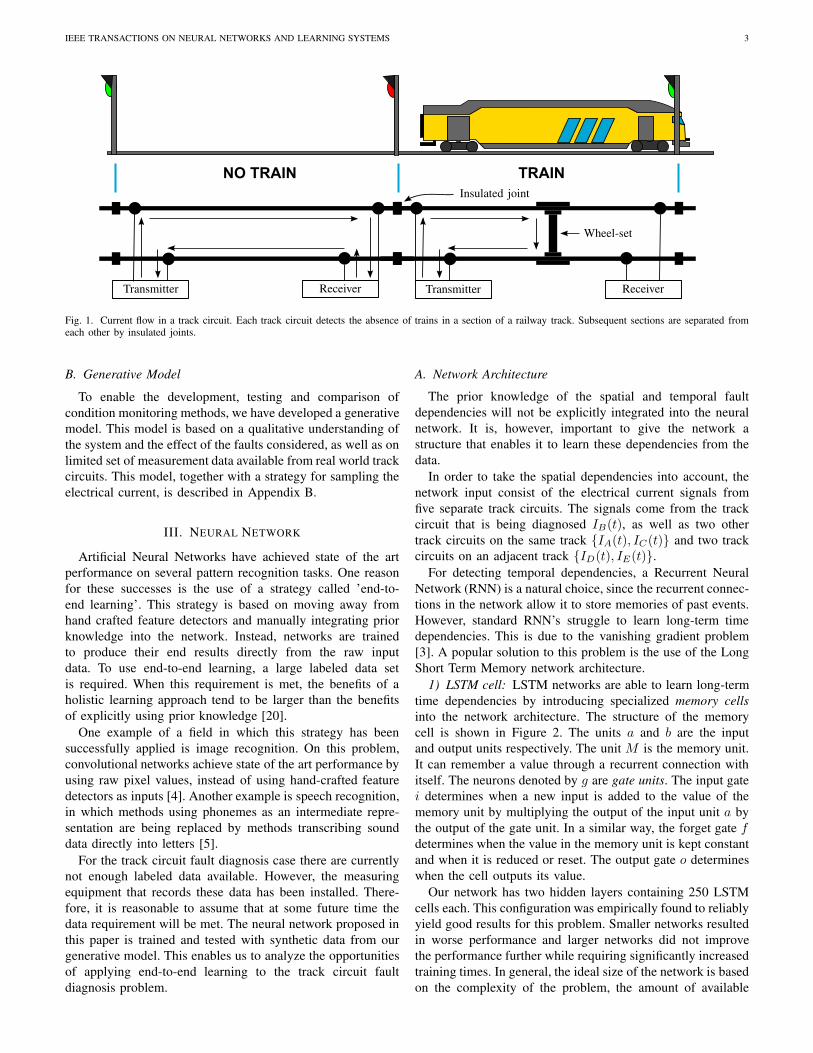
A track circuit works by using the rails in a track section as
conductors that connect a transmitter at one end of the section
to a receiver at the other end, as shown in Figure 1. When no
train is present in the section, the transmitter will energize a
relay in the receiver which indicates that the section is free.
When a train enters the section, the wheel-sets of the train
forms a short circuit as shown in Figure 1. This causes the
current flow through the receiver to decrease to a level where
the relay is no longer energized and the section is reported as
occupied.
The correct operation of a track circuit depends on the
electrical current through the receiver. In the absence of a train
in the section, the current must be high enough to energize the
relay. Conversely, in the presence of a train, the current must be
low enough so that the relay is de-energized. To maintain the
safety and availability of the railway network, it is important to
detect all possible faults in the system. Moreover, to schedule
preventive maintenance on the track circuits, it is important
to identify the fault type and to determine the development of
the fault severity over time.
A. Fault diagnosis
Every track circuit has different electrical properties which
results in different values of the ‘high’ current Ih(t) when no
train is present, and of the ‘low’ current Il(t) when a train is
present. Additionally, the transients between these values may
be different. The current levels also depend on environmental
influences and on the properties of the train passing through
the section. For these reasons, it is not possible to adequately
detect the presence of a fault by only considering the electrical
current I(t) during the passing of a single train. In this work
we consider the current signals from several track circuits in
the same geographic area, measured over a longer period of
time. This makes it possible to not only detect the presence of
a fault, but to also distinguish between different fault types.
The reasoning behind this approach is that different faults have
different spatial and temporal footprints [2]. The faults that are
considered in this paper are:
• Insulated joint defect
• Conductive object (across the insulated joints)
• Mechanical rail defect
• Electrical disturbance
• Ballast degradation
A description of these fault types, together with their spatial
and temporal footprints, is given in Appendix A.
IEEE TRANSACTIONS ON NEURAL NETWORKS AND LEARNING SYSTEMS 3
NO TRAIN TRAIN
Insulated joint
TransmitterTransmitter ReceiverReceiver
Wheel-set
Fig. 1. Current flow in a track circuit. Each track circuit detects the absence of trains in a section of a railway track. Subsequent sections are separated fromeach other by insulated joints.
B. Generative Model
To enable the development, testing and comparison of
condition monitoring methods, we have developed a generative
model. This model is based on a qualitative understanding of
the system and the effect of the faults considered, as well as on
limited set of measurement data available from real world track
circuits. This model, together with a strategy for sampling the
electrical current, is described in Appendix B.
III. NEURAL NETWORK
Artificial Neural Networks have achieved state of the art
performance on several pattern recognition tasks. One reason
for these successes is the use of a strategy called ’end-to-
end learning’. This strategy is based on moving away from
hand crafted feature detectors and manually integrating prior
knowledge into the network. Instead, networks are trained
to produce their end results directly from the raw input
data. To use end-to-end learning, a large labeled data set
is required. When this requirement is met, the benefits of a
holistic learning approach tend to be larger than the benefits
of explicitly using prior knowledge [20].
One example of a field in which this strategy has been
successfully applied is image recognition. On this problem,
convolutional networks achieve state of the art performance by
using raw pixel values, instead of using hand-crafted feature
detectors as inputs [4]. Another example is speech recognition,
in which methods using phonemes as an intermediate repre-
sentation are being replaced by methods transcribing sound
data directly into letters [5].
For the track circuit fault diagnosis case there are currently
not enough labeled data available. However, the measuring
equipment that records these data has been installed. There-
fore, it is reasonable to assume that at some future time the
data requirement will be met. The neural network proposed in
this paper is trained and tested with synthetic data from our
generative model. This enables us to analyze the opportunities
of applying end-to-end learning to the track circuit fault
diagnosis problem.
A. Network Architecture
The prior knowledge of the spatial and temporal fault
dependencies will not be explicitly integrated into the neural
network. It is, however, important to give the network a
structure that enables it to learn these dependencies from the
data.
In order to take the spatial dependencies into account, the
network input consist of the electrical current signals from
five separate track circuits. The signals come from the track
circuit that is being diagnosed IB(t), as well as two other
track circuits on the same track {IA(t), IC(t)} and two track
circuits on an adjacent track {ID(t), IE(t)}.
For detecting temporal dependencies, a Recurrent Neural
Network (RNN) is a natural choice, since the recurrent connec-
tions in the network allow it to store memories of past events.
However, standard RNN’s struggle to learn long-term time
dependencies. This is due to the vanishing gradient problem
[3]. A popular solution to this problem is the use of the Long
Short Term Memory network architecture.
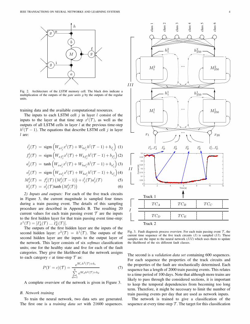
1) LSTM cell: LSTM networks are able to learn long-term
time dependencies by introducing specialized memory cells
into the network architecture. The structure of the memory
cell is shown in Figure 2. The units a and b are the input
and output units respectively. The unit M is the memory unit.
It can remember a value through a recurrent connection with
itself. The neurons denoted by g are gate units. The input gate
i determines when a new input is added to the value of the
memory unit by multiplying the output of the input unit a by
the output of the gate unit. In a similar way, the forget gate f
determines when the value in the memory unit is kept constant
and when it is reduced or reset. The output gate o determines
when the cell outputs its value.
Our network has two hidden layers containing 250 LSTM
cells each. This configuration was empirically found to reliably
yield good results for this problem. Smaller networks resulted
in worse performance and larger networks did not improve
the performance further while requiring significantly increased
training times. In general, the ideal size of the network is based
on the complexity of the problem, the amount of available
IEEE TRANSACTIONS ON NEURAL NETWORKS AND LEARNING SYSTEMS 4
g
g
g
a
b
M
h
i
o
f
Fig. 2. Architecture of the LSTM memory cell. The black dots indicate amultiplication of the outputs of the gate units g by the outputs of the regularunits.
training data and the available computational resources.
The inputs to each LSTM cell j in layer l consist of the
inputs to the layer at that time step xl(T ), as well as the
outputs of all LSTM cells in layer l at the previous time-step
hl(T − 1). The equations that describe LSTM cell j in layer
l are:
ilj(T ) = sigm(
Wxiljxl(T ) +Whil
jhl(T − 1) + bil
j
)
(1)
f lj(T ) = sigm
(
Wxf ljxl(T ) +Whf l
jhl(T − 1) + bf l
j
)
(2)
alj(T ) = tanh(
Wxaljxl(T ) +Whal
jhl(T − 1) + bal
j
)
(3)
olj(T ) = sigm(
Wxoljxl(T ) +Whol
jhl(T − 1) + bol
j
)
(4)
M lj(T ) = f l
j(T )(
M lj(T − 1)
)
+ ilj(T )alj(T ) (5)
hlj(T ) = olj(T )tanh
(
M lj(T )
)
(6)
2) Inputs and outputs: For each of the five track circuits
in Figure 3, the current magnitude is sampled four times
during a train passing event. The details of this sampling
procedure are described in Appendix B. The resulting 20
current values for each train passing event T are the inputs
to the first hidden layer for that train passing event time-step:
x1(T ) = [I1A(T ) ... I4E(T )].The outputs of the first hidden layer are the inputs of the
second hidden layer: x2(T ) = h1(T ). The outputs of the
second hidden layer are the inputs to the output layer of
the network. This layer consists of six softmax classification
units; one for the healthy state and five for each of the fault
categories. They give the likelihood that the network assigns
to each category c at time-step T as:
P (Y = c)(T ) =eWch
2(T )+bc
6∑
d=1
eWdh2(T )+bd
(7)
A complete overview of the network is given in Figure 3.
B. Network training
To train the neural network, two data sets are generated.
The first one is a training data set with 21600 sequences.
Time [s]
0 2 4 6 8 10 12
Curr
ent
[A]
0
0.05
0.1
0.15
0.2
0.25
0.3
0.35
0.4
...
...
...
TCA TCB TCC
TCD TCE
Track 1
Track 2
I1A..I4A I1B I2B I3B I4B I1C ..I
4E
x1 x20
M11 M1
250
h11 h1
250
M21 M2
250
h21 h2
250
clas
s1
clas
s2
clas
s3
clas
s4
clas
s5
clas
s6
I
II
III
Fig. 3. Fault diagnosis process overview. For each train passing event T , thecurrent time sequence of the five track circuits (I) is sampled (II). Thesesamples are the input to the neural network (III) which uses them to updatethe likelihood of the six different fault classes.
The second is a validation data set containing 600 sequences.
For each sequence the properties of the track circuits and
the properties of the fault are stochastically determined. Each
sequence has a length of 2000 train passing events. This relates
to a time period of 100 days. Note that although more trains are
likely to pass through the considered sections, it is important
to keep the temporal dependencies from becoming too long
term. Therefore, it might be necessary to limit the number of
train passing events per day that are used as network inputs.
The network is trained to give a classification of the
sequence at every time-step T . The target for this classification
IEEE TRANSACTIONS ON NEURAL NETWORKS AND LEARNING SYSTEMS 5
t(T ) is the healthy state, unless the sequence contains a fault
for which the severity at that time-step T is above 0.15. The
severity of the fault is between 0 and 1. A fault severity
of 0 will have no influence on the electrical current levels
and a fault severity of 1 will influence the current enough to
cause a failure, where the track circuit is no longer able to
function correctly. The value of 0.15 is chosen to detect the
faults as early as possible without having any false positive
fault detections. Based on the target classifications t(T ) the
network is trained to minimize the negative log likelihood loss
function:
l(T ) = −log(P (Y (T ) = t(T ))) (8)
The network is trained with the Back-Propagation Through
Time algorithm [21] on the sequences in the training data
set. The network is unrolled for 500 time-steps. First, the
network activations and outputs are calculated for these 500
time-steps. Then, moving backwards through time, the error
gradients are calculated and the weights are updated. Finally,
the activations of the network at the final time-step are used as
the initial network activations for the subsequent sub-sequence
of 500 time-steps. This process is repeated until all 2000 time-
steps in the sequence are processed. To improve efficiency, 56
sequences are processed simultaneously in a mini-batch using
Stochastic Gradient Descent.
During the training on the training data set, the performance
according to (8) on the validation data set is monitored.
When this performance stops improving the learning rate is
lowered. After the training is complete, the network weights
that resulted in the best performance on the validation data set
are used to test the network.
IV. RESULTS
To test the trained network a test data set is generated
containing 1500 sequences.
A. Prediction accuracy
To test the performance of the network, the test data set
is presented to the network. At the final time-step of the
sequences, the class that is assigned the highest probability
is compared to the correct diagnosis for that time-step.
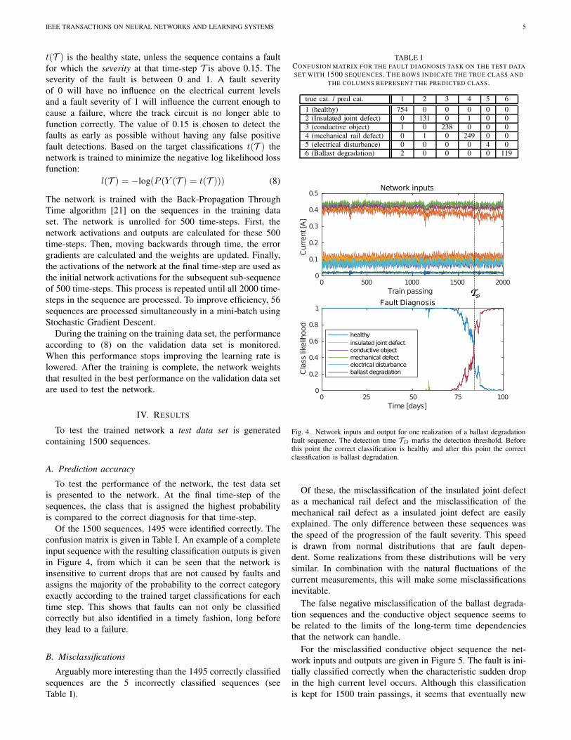
Of the 1500 sequences, 1495 were identified correctly. The
confusion matrix is given in Table I. An example of a complete
input sequence with the resulting classification outputs is given
in Figure 4, from which it can be seen that the network is
insensitive to current drops that are not caused by faults and
assigns the majority of the probability to the correct category
exactly according to the trained target classifications for each
time step. This shows that faults can not only be classified
correctly but also identified in a timely fashion, long before
they lead to a failure.
B. Misclassifications
Arguably more interesting than the 1495 correctly classified
sequences are the 5 incorrectly classified sequences (see
Table I).
TABLE ICONFUSION MATRIX FOR THE FAULT DIAGNOSIS TASK ON THE TEST DATA
SET WITH 1500 SEQUENCES. THE ROWS INDICATE THE TRUE CLASS AND
THE COLUMNS REPRESENT THE PREDICTED CLASS.
true cat. / pred cat. 1 2 3 4 5 6
1 (healthy) 754 0 0 0 0 0
2 (Insulated joint defect) 0 131 0 1 0 0
3 (conductive object) 1 0 238 0 0 0
4 (mechanical rail defect) 0 1 0 249 0 0
5 (electrical disturbance) 0 0 0 0 4 0
6 (Ballast degradation) 2 0 0 0 0 119
Fig. 4. Network inputs and output for one realization of a ballast degradationfault sequence. The detection time TD marks the detection threshold. Beforethis point the correct classification is healthy and after this point the correctclassification is ballast degradation.
Of these, the misclassification of the insulated joint defect
as a mechanical rail defect and the misclassification of the
mechanical rail defect as a insulated joint defect are easily
explained. The only difference between these sequences was
the speed of the progression of the fault severity. This speed
is drawn from normal distributions that are fault depen-
dent. Some realizations from these distributions will be very
similar. In combination with the natural fluctuations of the
current measurements, this will make some misclassifications
inevitable.
The false negative misclassification of the ballast degrada-
tion sequences and the conductive object sequence seems to
be related to the limits of the long-term time dependencies
that the network can handle.
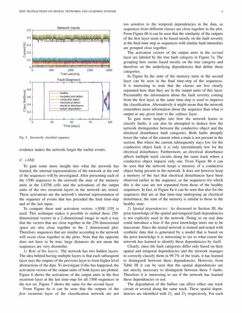
For the misclassified conductive object sequence the net-
work inputs and outputs are given in Figure 5. The fault is ini-
tially classified correctly when the characteristic sudden drop
in the high current level occurs. Although this classification
is kept for 1500 train passings, it seems that eventually new
IEEE TRANSACTIONS ON NEURAL NETWORKS AND LEARNING SYSTEMS 6
Fig. 5. Incorrectly classified sequence.
evidence makes the network forget the earlier events.
C. t-SNE
To gain some more insight into what the network has
learned, the internal representations of the network at the end
of the sequences will be investigated. After presenting each of
the 1500 sequences to the network the state of the memory
units in the LSTM cells and the activations of the output
units of the two recurrent layers in the network are stored.
These activations are the network’s internal representation of
the sequence of events that has preceded the final time-step
and of the last input.
To compare these unit activation vectors, t-SNE [19] is
used. This technique makes it possible to embed these 250-
dimensional vectors in a 2-dimensional image in such a way
that the vectors that are close together in the 250 dimensional
space are also close together in the 2 dimensional plot.
Therefore, sequences that are similar according to the network
will occur close together in the plots. Note that the opposite
does not have to be true; large distances do not mean the
sequences are very dissimilar.
1) Role of the layers: The network has two hidden layers.
The idea behind having multiple layers is that each subsequent
layer uses the outputs of the previous layer to form higher level
abstractions of the data. To investigate if this has happened, the
activation vectors of the output units of both layers are plotted.
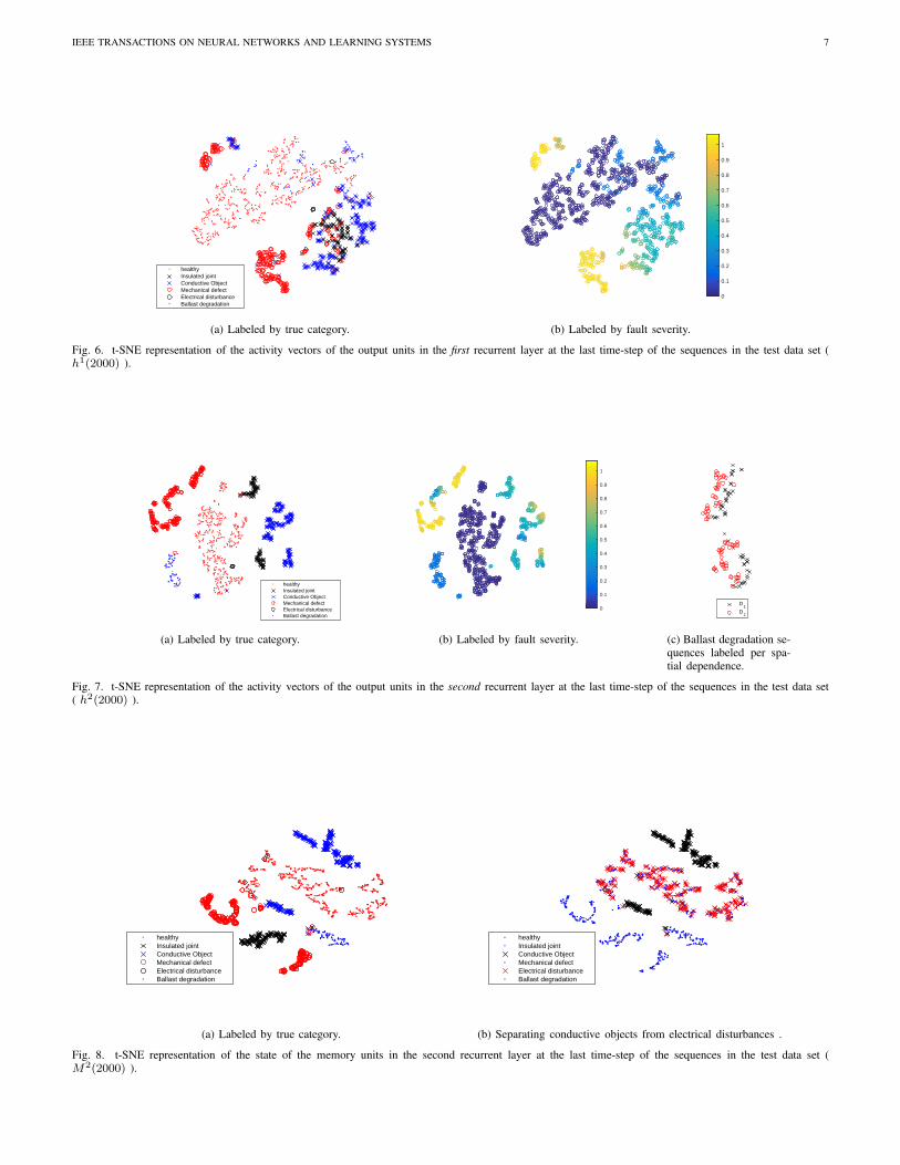
Figure 6 shows the activations of the output units in the first
recurrent layer at the last time-step for all 1500 sequences in
the test set. Figure 7 shows the same for the second layer.
From Figure 6a it can be seen that the outputs of the
first recurrent layer of the classification network are not
too sensitive to the temporal dependencies in the data, as
sequences from different classes are close together in the plot.
From Figure 6b it can be seen that the similarity of the outputs
of the first layer seem to be based mostly on the fault severity
at the final time-step as sequences with similar fault intensities
are grouped close together.
The activation vectors of the output units in the second
layer are labeled by the true fault category in Figure 7a. The
grouping here seems based mostly on the true category and
therefore on the underlying dependencies that define these
categories.
In Figure 8a the state of the memory units in the second
layer can be seen in the final time-step of the sequences.
It is interesting to note that the classes are less clearly
separated here than they are in the output units of this layer.
Presumably the information about the fault severity coming
from the first layer at the same time-step is used to improve
the classification. Alternatively it might mean that the network
remembers more information about the sequence than what is
output at any given time to the softmax layer.
To gain more insights into how the network learns to
classify faults, it can also be attempted to deduce how the
network distinguishes between the conductive object and the
electrical disturbance fault categories. Both faults abruptly
lower the value of the current when a train is not present in the
section. But where the current subsequently stays low for the
conductive object fault, it is only intermittently low for the
electrical disturbance. Furthermore, an electrical disturbance
affects multiple track circuits along the same track where a
conductive object impacts only one. From Figure 8b it can
be seen that the network keeps a memory of a conductive
object being present in the network. It does not however keep
a memory of the fact that electrical disturbances have been
observed earlier in the sequence, as the sequences for which
this is the case are not separated from those of the healthy
sequences. In fact, in Figure 8a it can be seen that also for the
sequences that are at that time-step undergoing an electrical
disturbance, the state of the memory is similar to those in the
healthy state.
2) Spatial dependencies: As discussed in Section III, the
prior knowledge of the spatial and temporal fault dependencies
is not explicitly used in the network. Doing so on real data
could introduce a bias if the prior knowledge turns out to be
inaccurate. Since the neural network is trained and tested with
synthetic data that is generated by a model that is based on
the prior knowledge it is interesting to see to what extent the
network has learned to identify these dependencies by itself.
Clearly, since the fault categories differ only based on their
spatial and temporal dependencies and the network manages
to correctly classify them in 99.7% of the trials, it has learned
to distinguish between these dependencies. However, from
Table III it can be seen that the spatial dependencies are
not strictly necessary to distinguish between these 5 faults.
Therefore it is interesting to see if the network has learned
these dependencies or not.
The degradation of the ballast can affect either one track
circuit or several along the same track. These spatial depen-
dencies are identified with D1 and D2 respectively. For each
IEEE TRANSACTIONS ON NEURAL NETWORKS AND LEARNING SYSTEMS 7
Fig. 6. t-SNE representation of the activity vectors of the output units in the first recurrent layer at the last time-step of the sequences in the test data set (h1(2000) ).
(c) Ballast degradation se-quences labeled per spa-tial dependence.
Fig. 7. t-SNE representation of the activity vectors of the output units in the second recurrent layer at the last time-step of the sequences in the test data set( h2(2000) ).
(b) Separating conductive objects from electrical disturbances .
Fig. 8. t-SNE representation of the state of the memory units in the second recurrent layer at the last time-step of the sequences in the test data set (M2(2000) ).
IEEE TRANSACTIONS ON NEURAL NETWORKS AND LEARNING SYSTEMS 8
sequence with a ballast degradation fault one of these options
is picked with equal probability. In Figure 7c the sequences
suffering from the ballast degradation fault are shown. It
appears from the plot that although these sequences are very
similar the network does distinguish between these spatial
dependencies.
V. CONVOLUTIONAL NETWORK COMPARISON
Besides LSTM RNNs, Convolutional Neural Networks
(CNNs) [22] are a popular choice for dealing with temporal
data [23]. In this section we compare our LSTM network with
a CNN.
The CNN that we consider is a feed-forward network that
takes all of the measurements of the past 2000 train-passings
on the five track circuits at once as an input and gives
the classification of the sequence at the most recent time-
step as an output. The CNN has two convolutional layers,
followed by a fully connected layer with Rectified Linear Unit
(ReLU) nonlinearities and a softmax output layer. Both con-
volutional layers consist of two sub-layers. The first performs
a convolution step where a series of kernels is convolved
with the inputs to the layer. The second sub-layer performs
a max-pooling step that takes the maximum activation of
the kernels over a certain time window. The max-pooling
operation introduces a limited invariance to the exact time at
which a certain input pattern was detected. This simplifies the
learning procedure and improves generalization. The kernel
widths and the number of filters were chosen based on prior
knowledge of the faults and in such a way that the total number
of parameters was approximately equal to that of the LSTM
network.
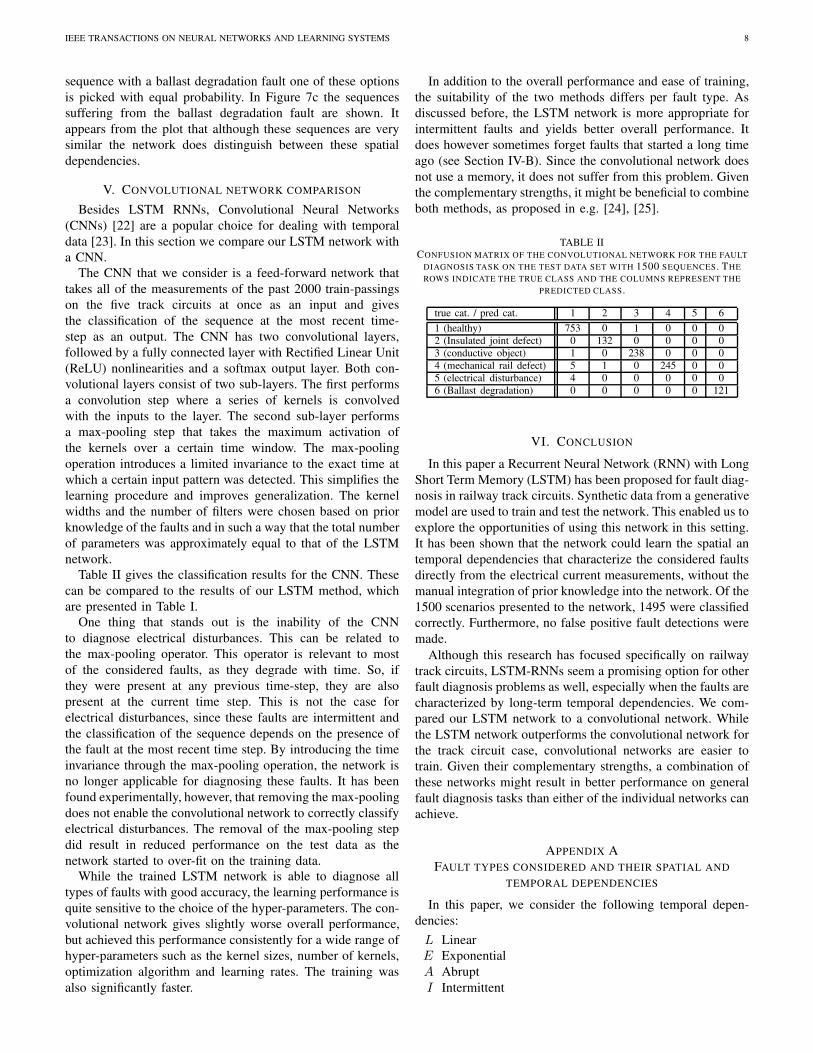
Table II gives the classification results for the CNN. These
can be compared to the results of our LSTM method, which
are presented in Table I.
One thing that stands out is the inability of the CNN
to diagnose electrical disturbances. This can be related to
the max-pooling operator. This operator is relevant to most
of the considered faults, as they degrade with time. So, if
they were present at any previous time-step, they are also
present at the current time step. This is not the case for
electrical disturbances, since these faults are intermittent and
the classification of the sequence depends on the presence of
the fault at the most recent time step. By introducing the time
invariance through the max-pooling operation, the network is
no longer applicable for diagnosing these faults. It has been
found experimentally, however, that removing the max-pooling
does not enable the convolutional network to correctly classify
electrical disturbances. The removal of the max-pooling step
did result in reduced performance on the test data as the
network started to over-fit on the training data.
While the trained LSTM network is able to diagnose all
types of faults with good accuracy, the learning performance is
quite sensitive to the choice of the hyper-parameters. The con-
but achieved this performance consistently for a wide range of
hyper-parameters such as the kernel sizes, number of kernels,
optimization algorithm and learning rates. The training was
also significantly faster.
In addition to the overall performance and ease of training,
the suitability of the two methods differs per fault type. As
discussed before, the LSTM network is more appropriate for
intermittent faults and yields better overall performance. It
does however sometimes forget faults that started a long time
ago (see Section IV-B). Since the convolutional network does
not use a memory, it does not suffer from this problem. Given
the complementary strengths, it might be beneficial to combine
both methods, as proposed in e.g. [24], [25].
TABLE IICONFUSION MATRIX OF THE CONVOLUTIONAL NETWORK FOR THE FAULT
DIAGNOSIS TASK ON THE TEST DATA SET WITH 1500 SEQUENCES. THE
ROWS INDICATE THE TRUE CLASS AND THE COLUMNS REPRESENT THE
PREDICTED CLASS.
true cat. / pred cat. 1 2 3 4 5 6
1 (healthy) 753 0 1 0 0 0
2 (Insulated joint defect) 0 132 0 0 0 0
3 (conductive object) 1 0 238 0 0 0
4 (mechanical rail defect) 5 1 0 245 0 0
5 (electrical disturbance) 4 0 0 0 0 0
6 (Ballast degradation) 0 0 0 0 0 121
VI. CONCLUSION
In this paper a Recurrent Neural Network (RNN) with Long
Short Term Memory (LSTM) has been proposed for fault diag-
nosis in railway track circuits. Synthetic data from a generative
model are used to train and test the network. This enabled us to
explore the opportunities of using this network in this setting.
It has been shown that the network could learn the spatial an
temporal dependencies that characterize the considered faults
directly from the electrical current measurements, without the
manual integration of prior knowledge into the network. Of the
1500 scenarios presented to the network, 1495 were classified
correctly. Furthermore, no false positive fault detections were
made.
Although this research has focused specifically on railway
track circuits, LSTM-RNNs seem a promising option for other
fault diagnosis problems as well, especially when the faults are
characterized by long-term temporal dependencies. We com-
pared our LSTM network to a convolutional network. While
the LSTM network outperforms the convolutional network for
the track circuit case, convolutional networks are easier to
train. Given their complementary strengths, a combination of
these networks might result in better performance on general
fault diagnosis tasks than either of the individual networks can
achieve.
APPENDIX A
FAULT TYPES CONSIDERED AND THEIR SPATIAL AND
TEMPORAL DEPENDENCIES
In this paper, we consider the following temporal depen-
dencies:
L Linear
E Exponential
A Abrupt
I Intermittent
IEEE TRANSACTIONS ON NEURAL NETWORKS AND LEARNING SYSTEMS 9
Some faults that depend on time in a linear or exponential
fashion can also be distinguished by the relative speed of the
dependence. The spatial dependencies considered are:
Dc: The fault only affects the current in one track circuit.
Dt: The fault affects the current in more track circuits on the
same track.
Da: The fault affects the current of all track circuits in a
certain area.
A. Fault types considered
In this paper, we consider a set of five different faults as
described below. Table III gives a summary of the spatial and
temporal dependencies per fault type.
TABLE IIIFAULT TYPES AND THEIR SPATIAL AND TEMPORAL DEPENDENCIES.
Fault type Spatial Temporal Fault rate
Insulated joint defect D1 L ∨ E intermediate
Conductive object D1 A -
Mechanical rail defect D1 E high
Electrical disturbance D2 I -
Ballast degradation D1 ∨D2 L ∨ E low
1) Insulation imperfections: The sections of a railway track
are electrically separated by insulated joints. When these joints
wear out, the track circuit current of one section can leak into
the adjacent section. The system is designed to be failsafe,
ensuring that the section that the current leaks into will not
be identified as free because of this leakage. However, the
current level in the section that the signal leaks out of will
drop, potentially causing the section to be incorrectly identified
as being occupied.
The effect of this fault will only be noticed in the section
that the current leaks out of. As trains pass over the damaged
joint the defect will gradually get worse. The fault severity is
therefore expected to increase either linearly or exponentially.
A conductive object placed over an insulated joint has a
similar effect as the joint defect. In this case, however, the
effect will occur abruptly and will not deteriorate over time.
2) Rail conductance impairments: The current travels
through the rails from the transmitter to the receiver. When
the impedance of this path increases, the current level in the
receiver will decrease. One fault that can cause this problem is
a mechanical defect in the rail. This fault would be specific to a
single section and will increase exponentially over time as each
passing train would cause greater damage to the deteriorating
rail.
Another reason for the impedance of the rails to increase
is the influence of disturbance currents. An example of this is
when the track is saturated with traction currents. This problem
occurs intermittently and affects several track circuits along the
same track.
3) Ballast degradation: Some current will always leak
through the ballast between the rails in the section. The
amount of current that leaks through the ballast depends on
the impedance of the ballast. This impedance varies as a
consequence of environmental conditions.
The ballast can also degrade over time, leading to a linear
or exponential reduction in the magnitude of the signaling
current when no train is present in the section. This effect
would be noticeable in one or more sections along the same
track. Compared to other faults this fault would likely develop
more slowly.
APPENDIX B
GENERATIVE MODEL
To create a model that generates the amplitude of the
electrical current I(t) in the receiver of a track circuit as a
train passes through the section, a data set of measurement
sequences from T = 30000 train passings has been studied.
A mathematical model that was found to accurately describe
these measurements was then fitted to the data. This model is
based on four phases during a train passing event:
• Phase 1: Between t0 and t1 the train has not yet arrived
in the section. During this phase the current I(t) through
the receiver should therefore be at the high level: I(t) =Ih.
• Phase 2: At t = t1 the first wheel-set of the train
enters the section. If the resistance of the wheel-set
short circuit is low enough this should result in a very
quick drop of I(t) to its low value Il. However, in a
large portion of the samples in the data set the current
drop is more gradual. By fitting a number of samples
from three different track circuits to several equations
for step responses it was found that this phase could be
accurately and robustly described by an equation of the
form I(t) = α1e−τα1(t−t1) + β1e
−τβ1(t−t1) .
• Phase 3: Although ideally I(t) = Il should hold until
the last wheel-set of the train leaves the section, in the
majority of the samples in the data set the current starts
to increase before this time. The curve between t = t2where the current is at the lowest level and t = t3 where
the last wheel-set leaves the section can in almost all
cases be accurately described by a function of the form:
I(t) = α2eτα2(t−t2) + β2e
τβ2(t−t2) .
• Phase 4: After the last wheel-set leaves the section
at t = t3 the current I(t) quickly increases to a value
near Ih. On some of the samples some overshoot is
observed and on some samples a trend after the step is
observed. Although a first order step response was found
to accurately describe many of the samples, a function of
the form I(t) = α3e−τα3(t−t3)+β3e
τβ3(t−t3) was found to
represent these less common cases as well and is therefore
chosen for the initial fitted model.
In Figure 3-II it can be seen that this model accurately
describes the development of the current over time I(t) during
a train passing event T . This model was fitted to all of the
measured data sequences. By analyzing the distributions of the
values of the fitted model parameters it was possible to create
a simplified model with only a minimal sacrifice to the fitting
IEEE TRANSACTIONS ON NEURAL NETWORKS AND LEARNING SYSTEMS 10
accuracy. This model is given by
I(t) = Il +∆Imax·
1 for t < t1
(1 −R)e−τα1(t−t1) +Re−τβ1(t−t1) for t1 ≤ t < t2
(t− t2)∆I3
(t3−t2)for t2 ≤ t < t3
1− e−τ3(t−t3) for t ≥ t3(9)
with the following values for the time-constants:
τα1 = 9.25τβ1 = 1.7τ3 = 12.5
and
∆Imax = Ih − Il .
In this simplified model the properties of the track circuit and
the passing train are now represented by the four variables
Ih, Il, R and ∆I3. By fitting the simplified model to the
measured data and investigating the environmental conditions
at the time of the measurements, the dependencies of these
four variables on several sources of normal variation were
found. These sources include precipitation, the time of day
and train specific variations.
As these dependencies only explain part of the observed
variation in the measured data, several short and long-term
stochastic variations have been added to the model that affect
both single track circuits and several track circuits in an area.
Additionally, the nominal parameters of the track circuits as
well as the sensitivity of each track circuit to the sources
of variation are determined stochastically for each track cir-
cuit. This ensures that the synthetic data that the generative
model produces contains comparable types of variation to
the true measurement data. This makes it possible to not
only determine the robustness of the condition monitoring
method to these variations, but also its ability to pick up more
subtle dependencies in the data and use them. For example,
weather influences will affect all track circuits in a small
area. By correctly identifying this influence the effects on the
measured signal could be filtered out, improving the condition
monitoring performance.
A. Sampling strategy
The faults that can affect the performance of the track
circuits will in most cases change the values of the parameters
Ih, Il, R and ∆I3 very slowly over time. It is therefore impor-
tant to sample the current I(t) in a way that is informative of
these values while taking as few samples per train passing
T as possible to ensure a high information density in the
measurements.
Based on equation 9 the following sampling times are used:
• t1: Just before the train arrives in the section: when the
amplitude of the track circuit current is the highest Ih.
• t1 +0.35s: The value of the current I(t) at 0.35 seconds
after the first wheel set of the train enters the section is
most instructive about the value of parameter R.
• t2: When the current is at its lowest value Il, about
halfway through the train passing event.
• t3: Just before the last wheel set of the train leaves the
section. This measurement gives ∆I3.
These four sampling times are indicated in Figure 3 - II . As
the simplified model of equation 9 fits the measured data well,
these sampling times should also work for real measurement
data.
To ensure a high enough information density for the Ar-
tificial Neural Network to learn the long-term temporal fault
dependencies, these four current values are observed for all
five considered track circuits and presented as one input time
step T to the network. This means that two trains (one on
each track) should pass through the area before a new input
is presented to the network.
REFERENCES
[1] J. Chen, C. Roberts, and P. Weston, “Fault detection and diagnosis forrailway track circuits using neuro-fuzzy systems,” Control Engineering
Practice, vol. 16, no. 5, pp. 585–596, 2008.
[2] K. Verbert, B. De Schutter, and R. Babuška, “Exploiting spatial andtemporal dependencies to enhance fault diagnosis: Application to railwaytrack circuits,” in Proceedings of the 2015 European Control Conference,Linz, Austria, Jul. 2015, pp. 3052–3057.
[3] S. Hochreiter and J. Schmidhuber, “Long short-term memory,” Neural
computation, vol. 9, no. 8, pp. 1735–1780, 1997.
[4] R. Wu, S. Yan, Y. Shan, Q. Dang, and G. Sun, “Deep image: Scalingup image recognition,” arXiv preprint arXiv:1501.02876, 2015.
[5] A. Y. Hannun, C. Case, J. Casper, B. C. Catanzaro, G. Diamos,E. Elsen, R. Prenger, S. Satheesh, S. Sengupta, A. Coates, and A. Y. Ng,“Deep speech: Scaling up end-to-end speech recognition,” CoRR, vol.abs/1412.5567, 2014. [Online]. Available: http://arxiv.org/abs/1412.5567
[6] L. Oukhellou, A. Debiolles, T. Denoeux, and P. Aknin, “Fault diag-nosis in railway track circuits using Dempster-Shafer classifier fusion,”Engineering Applications of Artificial Intelligence, vol. 23, no. 1, pp.117–128, 2010.
[7] Z. L. Cherfi, L. Oukhellou, E. Côme, T. Denœux, and P. Aknin, “Partiallysupervised independent factor analysis using soft labels elicited frommultiple experts: Application to railway track circuit diagnosis,” Soft
computing, vol. 16, no. 5, pp. 741–754, 2012.
[8] M. Sandidzadeh and M. Dehghani, “Intelligent condition monitoring ofrailway signaling in train detection subsystems,” Journal of Intelligent
and Fuzzy Systems, vol. 24, no. 4, pp. 859–869, 2013.
[9] S. Sun and H. Zhao, “Fault diagnosis in railway track circuits usingsupport vector machines,” in Proceedings of the 12th International
Conference on Machine Learning and Applications, vol. 2, Miami, FL,2013, pp. 345–350.
[10] Z. Lin-Hai, W. Jian-Ping, and R. Yi-Kui, “Fault diagnosis for trackcircuit using AOK-TFRs and AGA,” Control Engineering Practice,vol. 20, no. 12, pp. 1270–1280, 2012.
[11] S. Ntalampiras, “Fault identification in distributed sensor networks basedon universal probabilistic modeling,” IEEE Transactions on Neural
Networks and Learning Systems, vol. 26, no. 9, pp. 1939–1949, 2015.
[12] M. M. Gardner, J.-C. Lu, R. S. Gyurcsik, J. J. Wortman, B. E. Hornung,H. H. Heinisch, E. A. Rying, S. Rao, J. C. Davis, and P. K. Mozumder,“Equipment fault detection using spatial signatures,” IEEE Transactions
on Components, Packaging, and Manufacturing Technology, Part C,vol. 20, no. 4, pp. 295–304, 1997.
[13] J. Chen, S. Kher, and A. Somani, “Distributed fault detection of wirelesssensor networks,” in Proceedings of the 2006 workshop on Dependability
issues in wireless ad hoc networks and sensor networks. ACM, 2006,pp. 65–72.
[14] G. E. Hinton, S. Osindero, and Y.-W. Teh, “A fast learning algorithm fordeep belief nets,” Neural computation, vol. 18, no. 7, pp. 1527–1554,2006.
[15] J. Sun, R. Wyss, A. Steinecker, and P. Glocker, “Automated faultdetection using deep belief networks for the quality inspection ofelectromotors,” tm-Technisches Messen, vol. 81, no. 5, pp. 255–263,2014.
IEEE TRANSACTIONS ON NEURAL NETWORKS AND LEARNING SYSTEMS 11
[16] C. Shang, F. Yang, D. Huang, and W. Lyu, “Data-driven soft sensordevelopment based on deep learning technique,” Journal of Process
Control, vol. 24, no. 3, pp. 223–233, 2014.[17] O. Obst, “Distributed fault detection in sensor networks using a recurrent
neural network,” arXiv preprint arXiv:0906.4154, 2009.[18] H. C. Cho, J. Knowles, M. S. Fadali, and K. S. Lee, “Fault detection
and isolation of induction motors using recurrent neural networksand dynamic bayesian modeling,” Control Systems Technology, IEEE
Transactions on, vol. 18, no. 2, pp. 430–437, 2010.[19] L. Van der Maaten and G. Hinton, “Visualizing data using t-sne,” Journal
of Machine Learning Research, vol. 9, no. 2579-2605, p. 85, 2008.[20] A. Graves and N. Jaitly, “Towards end-to-end speech recognition with
recurrent neural networks,” in Proceedings of the 31st International
Conference on Machine Learning (ICML-14), 2014, pp. 1764–1772.[21] P. J. Werbos, “Backpropagation through time: what it does and how to
do it,” Proceedings of the IEEE, vol. 78, no. 10, pp. 1550–1560, 1990.[22] Y. LeCun and Y. Bengio, “Convolutional networks for images, speech,
and time series,” The handbook of brain theory and neural networks,vol. 3361, no. 10, p. 1995, 1995.
[23] M. Längkvist, L. Karlsson, and A. Loutfi, “A review of unsupervisedfeature learning and deep learning for time-series modeling,” Pattern
Recognition Letters, vol. 42, pp. 11–24, 2014.[24] T. N. Sainath, O. Vinyals, A. Senior, and H. Sak, “Convolutional, long
short-term memory, fully connected deep neural networks,” in Acoustics,
Speech and Signal Processing (ICASSP), 2015 IEEE International
Conference on. IEEE, 2015, pp. 4580–4584.[25] L. Deng and J. C. Platt, “Ensemble deep learning for speech recogni-
tion.” in INTERSPEECH, 2014, pp. 1915–1919.
T. de Bruin received the B.Sc. degree in MechanicalEngineering in 2012 and the M.Sc. degree in Sys-tems and Control in 2015 from the Delft Universityof Technology, Delft, The Netherlands. He is cur-rently working toward the Ph.D. degree at the DelftCenter for Systems and Control, Delft Universityof Technology. His research interests include neuralnetworks, reinforcement learning, and robotics.
K. Verbert received the B.Eng. degree (cum laude)in Human Kinetic Technology from the Hague Uni-versity of Applied Sciences, The Hague, The Nether-lands, in 2009 and the M.Sc. degree (cum laude)in Control Engineering from the Delft University ofTechnology, Delft, The Netherlands, in 2012. Sheis currently working toward the Ph.D. degree at theDelft Center for Systems and Control, Delft Uni-versity of Technology. Her current research interestsinclude fault diagnosis, maintenance optimization,friction compensation, and (human) motion control.
R. Babuška received the M.Sc. degree (with hon-ors) in control engineering from the Czech Tech-nical University in Prague, in 1990, and the Ph.D.degree (cum laude) from the Delft University ofTechnology, the Netherlands, in 1997. He has hadfaculty appointments at the Czech Technical Univer-sity Prague and at the Electrical Engineering Facultyof the Delft University of Technology. Currently, heis a Professor of Intelligent Control and Robotics atthe Delft Center for Systems and Control. He is alsothe director of the TU Delft Robotics Institute. His
research interests include reinforcement learning, neural and fuzzy systems,nonlinear identification, state-estimation, model-based and adaptive controland dynamic multi-agent systems. He has been working on applications ofthese techniques in the fields of robotics, mechatronics, and aerospace.