Delft3D model based alongshore sediment transport rates at Pesalai, Gurunagar, Point Pedro and Mullaitivu, Sri Lanka (Phase 2 Final Report)

October 2016

Sri: Northern Province Sustainable Fisheries

Development Project

Prepared by UNESCO-HE for the Asian Development Bank. This sediment transport monitoring report is a document of the UNESCO-HE. The views

expressed herein do not necessarily represent those of ADB's Board of Directors, Management,

or staff, and may be preliminary in nature. Your attention is directed to the “terms of use” section of this website.

In preparing any country program or strategy, financing any project, or by making any

designation of or reference to a particular territory or geographic area in this document, the

Asian Development Bank does not intend to make any judgments as to the legal or other status

of any territory or area

i

Delft3D model based alongshore sediment transport rates at Pesalai, Gurunagar, Point Pedro and Mullaitivu, Sri Lanka (Phase 2 Final Report)

Project :

COMPREHENSIVE MODELING OF LONGSHORE SEDIMENT TRANSPORT AT PESALAI,

GURUNAGAR, POINT PEDRO AND MULLAITIVU, SRI LANKA

October 2016

ii

Table of Contents Table of Contents .....................................................................................................................................ii

Executive Summary .................................................................................................................................. v

1. Introduction ..................................................................................................................................... 1

1.1. Background .............................................................................................................................. 1

1.2. Problem description ................................................................................................................ 1

1.3. Objectives ................................................................................................................................ 1

1.4. Approach ................................................................................................................................. 1

1.5. Outline ..................................................................................................................................... 1

2. Site description and data ................................................................................................................. 2

2.1. Sri Lanka .................................................................................................................................. 2

2.2. Pesalai ...................................................................................................................................... 2

2.2.1. Site description ................................................................................................................ 2

2.2.2. Bathymetric data ............................................................................................................. 3

2.2.3. Sediment data ................................................................................................................. 4

2.2.4. Layout .............................................................................................................................. 5

2.3. Gurunagar ................................................................................................................................ 6

2.3.1. Site description ................................................................................................................ 6

Site visit ....................................................................................................................................... 6

2.3.2. Bathymetric data ............................................................................................................. 7

2.3.3. Sediment data ................................................................................................................. 8

2.3.4. Layout .............................................................................................................................. 9

2.4. Point Pedro ............................................................................................................................ 10

2.4.1. Site description .............................................................................................................. 10

Site visit ..................................................................................................................................... 11

2.4.2. Bathymetric data ........................................................................................................... 12

2.4.3. Sediment data ............................................................................................................... 13

2.4.4. Layout ............................................................................................................................ 13

2.5. Mullaitivu ............................................................................................................................... 14

2.5.1. Site description .............................................................................................................. 14

2.5.2. Bathymetric data ........................................................................................................... 15

2.5.3. Sediment data ............................................................................................................... 16

iii

2.5.4. Layout ............................................................................................................................ 16

2.6. Wave data.............................................................................................................................. 16

3. Model setup .................................................................................................................................. 17

3.1. Model description and settings ............................................................................................. 17

3.2. Pesalai .................................................................................................................................... 18

3.2.1. Results ........................................................................................................................... 21

3.3. Gurunagar .............................................................................................................................. 26

3.3.1. Results ........................................................................................................................... 28

3.4. Point Pedro ............................................................................................................................ 30

3.4.1. Results ........................................................................................................................... 32

3.5. Mullaitivu ............................................................................................................................... 33

3.5.1. Results ........................................................................................................................... 38

4. Conclusions and recommendations .............................................................................................. 41

4.1. General .................................................................................................................................. 41

4.1.1. Conclusions .................................................................................................................... 41

4.1.2. Recommendations ......................................................................................................... 41

4.2. Pesalai .................................................................................................................................... 42

4.3. Gurunagar .............................................................................................................................. 42

4.4. Point Pedro ............................................................................................................................ 42

4.5. Mullaitivu ............................................................................................................................... 43

5. References ..................................................................................................................................... 44

A. Wave modeling .............................................................................................................................. 45

A.1 Objectives and approach............................................................................................................. 45

A.2 SWAN wave model ...................................................................................................................... 45

A.3 Wave data: ERA-interim .............................................................................................................. 46

A.4 Model set-up ............................................................................................................................... 48

A.5 Boundary conditions: scenarios .................................................................................................. 50

A.6 Model results .............................................................................................................................. 51

B. Tidal modeling ............................................................................................................................... 56

iv

v

Executive Summary

In Nov. 2015 , under the Asian Development Bank (ADB) – UNESCO-IHE partnership, UNESCO-IHE was

invited to to perform a detailed, state-of-the-art numerical modelling study to comprehensively

assess the present-day longshore sediment transport regime along the North coast of Sri Lanka to

inform the planned construction of four fishery harbours along the North coast of Sri Lanka.

The overall study consists of two Phases. Phase 1 will develop a coarse hydrodynamic model to

simulate the dominant large scale wave, wind and tide driven circulation patterns and use those results

to design and implement a bathymetric survey of the 4 study areas (Pesalai, Gurunagar, Point Pedro

and Mullaitivu) which will feed into Phase 2. Phase 2 will perform detailed coastal sediment transport

modelling for the 4 sites, and assess the prevailing alongshore sediment transport regime in the 4 study

areas.

This report constitutes the deliverable of the 2nd phase of this project and documents the details

pertaining to the application of the Delft3D/SWAN model suite to the 4 study areas, and provides

estimates of net and gross longshore sediment transport rates and recommendations for the 3 sites.

Note that the construction of the harbour at Mullaitivu was abandoned during the course of this study,

and hence only a sediment budget is provided for this site.

Detailed Delft3D/SWAN models, based on the bathymetric surveys undertaken in Phase 1 of this study,

were setup for each of the study sites. Wave input data for the detailed (i.e. local) models were derived

from large scale wave and tide models forced with global and regional hindcast models. The longshore

sediment transport rates predicted by the detailed Delft3D/SWAN models were verified with the one-

line model UNIBEST-LT, and a combination of field observations and Google Earth imagery. The

longshore sediment transport (LST) rates thus estimated for the 4 sites are shown below in Table E1.

Table E1 Annual longshore sediment transport rates at proposed Pesalai, Gurunagar and Point Pedro harbour locations

Location Net annual alongshore sediment

transport rate (m3/year)

Gross annual alongshore

sediment transport rate (m3/year)

Pesalai 10,000 from east to west 1,000 from west to east

11,000 from east to west

Gurunagar 5,000 from west to east 5,000 from west to east

Point Pedro 30,000-150,000 from east to west 30,000-150,000 from east to west

Mullaitivu North of inlet 10,000-65,000 to

north

South of inlet 30,000(to south)-

20,000 (to north)

North of inlet 10,000-65,000 to

north

South of inlet 30,000 to north-

35,000 to south

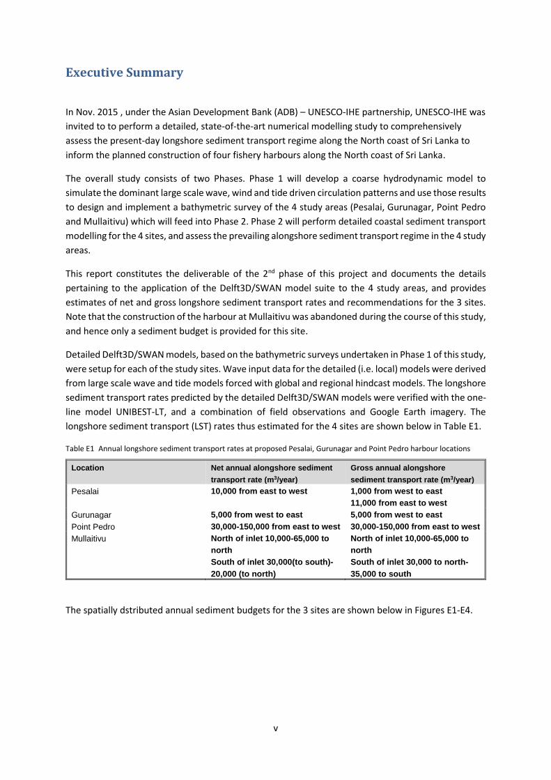
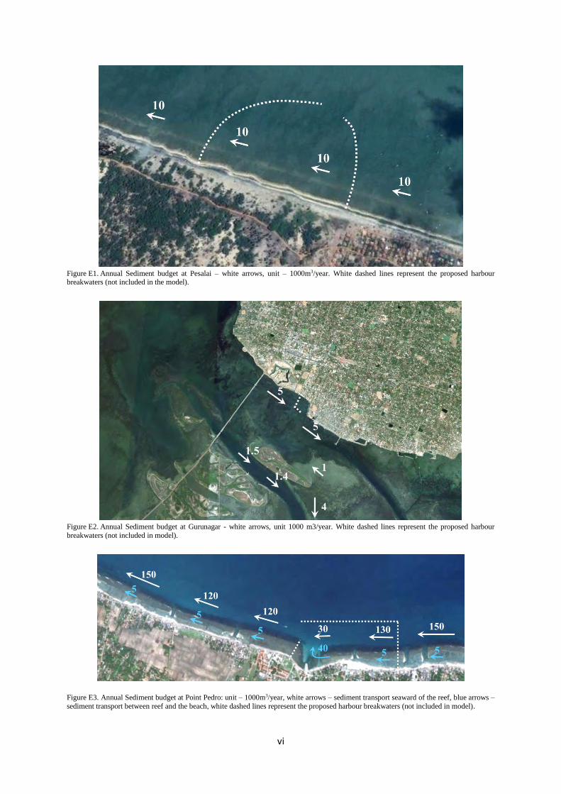
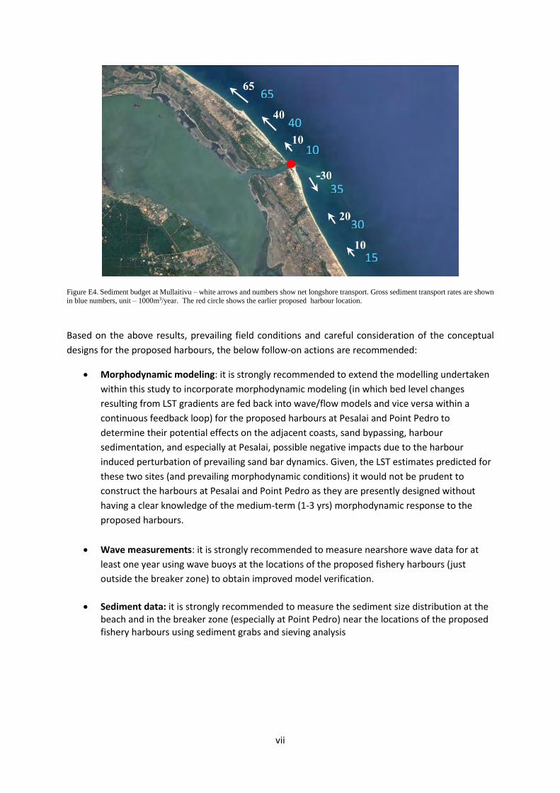
The spatially dstributed annual sediment budgets for the 3 sites are shown below in Figures E1-E4.

vi

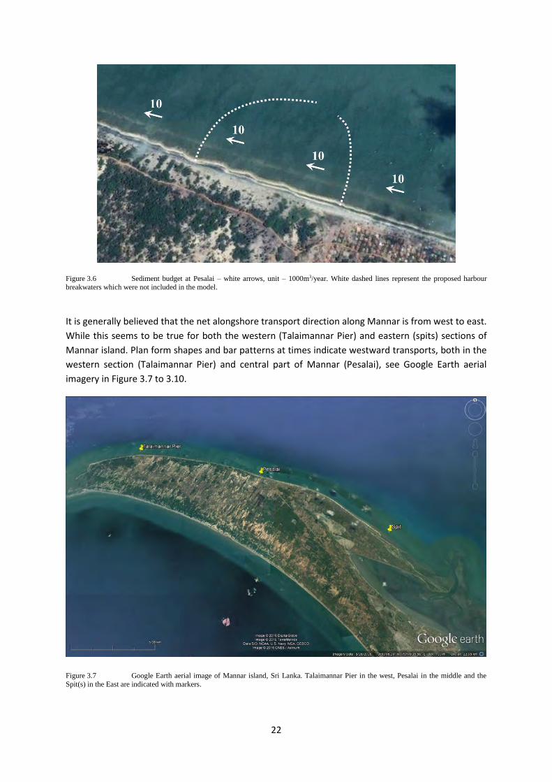
Figure E1. Annual Sediment budget at Pesalai – white arrows, unit – 1000m3/year. White dashed lines represent the proposed harbour

breakwaters (not included in the model).

Figure E2. Annual Sediment budget at Gurunagar - white arrows, unit 1000 m3/year. White dashed lines represent the proposed harbour

breakwaters (not included in model).

Figure E3. Annual Sediment budget at Point Pedro: unit – 1000m3/year, white arrows – sediment transport seaward of the reef, blue arrows –

sediment transport between reef and the beach, white dashed lines represent the proposed harbour breakwaters (not included in model).

vii

Figure E4. Sediment budget at Mullaitivu – white arrows and numbers show net longshore transport. Gross sediment transport rates are shown

in blue numbers, unit – 1000m3/year. The red circle shows the earlier proposed harbour location.

Based on the above results, prevailing field conditions and careful consideration of the conceptual

designs for the proposed harbours, the below follow-on actions are recommended:

Morphodynamic modeling: it is strongly recommended to extend the modelling undertaken

within this study to incorporate morphodynamic modeling (in which bed level changes

resulting from LST gradients are fed back into wave/flow models and vice versa within a

continuous feedback loop) for the proposed harbours at Pesalai and Point Pedro to

determine their potential effects on the adjacent coasts, sand bypassing, harbour

sedimentation, and especially at Pesalai, possible negative impacts due to the harbour

induced perturbation of prevailing sand bar dynamics. Given, the LST estimates predicted for

these two sites (and prevailing morphodynamic conditions) it would not be prudent to

construct the harbours at Pesalai and Point Pedro as they are presently designed without

having a clear knowledge of the medium-term (1-3 yrs) morphodynamic response to the

proposed harbours.

Wave measurements: it is strongly recommended to measure nearshore wave data for at

least one year using wave buoys at the locations of the proposed fishery harbours (just

outside the breaker zone) to obtain improved model verification.

Sediment data: it is strongly recommended to measure the sediment size distribution at the

beach and in the breaker zone (especially at Point Pedro) near the locations of the proposed

fishery harbours using sediment grabs and sieving analysis

65

40

10

35

30

15

1

1. Introduction

1.1. Background

UNESCO-IHE Delft has been commissioned a two phase study by the Asian Development Bank (ADB)

to provide longshore sediment transport rates at four potential harbour sites in Northern Sri Lanka.

This report relates to Phase 2 of the study which provides estimates of prevailing alongshore

sediment transport rates using state of the art numerical modelling. To ensure timely project

delivery, UNESCO-IHE obtained modelling support from Deltares in this part of the study.

1.2. Problem description

The proposed construction of fishery harbours at Pesalai, Gurunagar, Point Pedro and Mullaitivu will

inevitably involve the construction of jetties and/or breakwaters which will interrupt the natural

wave driven sediment transport along the coastline. Both the functionality of the harbours and the

adjacent coast may face severe negative impacts if the design of the harbour jetties/breakwaters

does not take into account the natural prevailing alongshore sediment transport rates in their

vicinity. The main potential negative impacts that may be felt are; (a) rapid shoaling of the harbour

entrance and basin, and (2) severe wave driven erosion of the adjacent coastline. Oluvil and Kirinda

harbours which were recently constructed without due consideration of the prevailing alongshore

sediment transport regime in the area are good examples of the manifestation of such negative

impacts. To ensure that the proposed harbours at Pesalai, Gurunagar, Point Pedro and Mullaitivu do

not face the same fate, it is essential to have reliable estimates of prevailing alongshore sediment

transport rates in these areas.

1.3. Objectives

The objective of this study is to provide reliable estimates of prevailing alongshore sediment

transport rates at the location of the proposed harbours at Pesalai, Gurunagar, Point Pedro and

Mullaitivu, Sri Lanka. This report provides estimates of alongshore sediment transport rates at the 4

locations using state-of-the-art coastal numerical models.

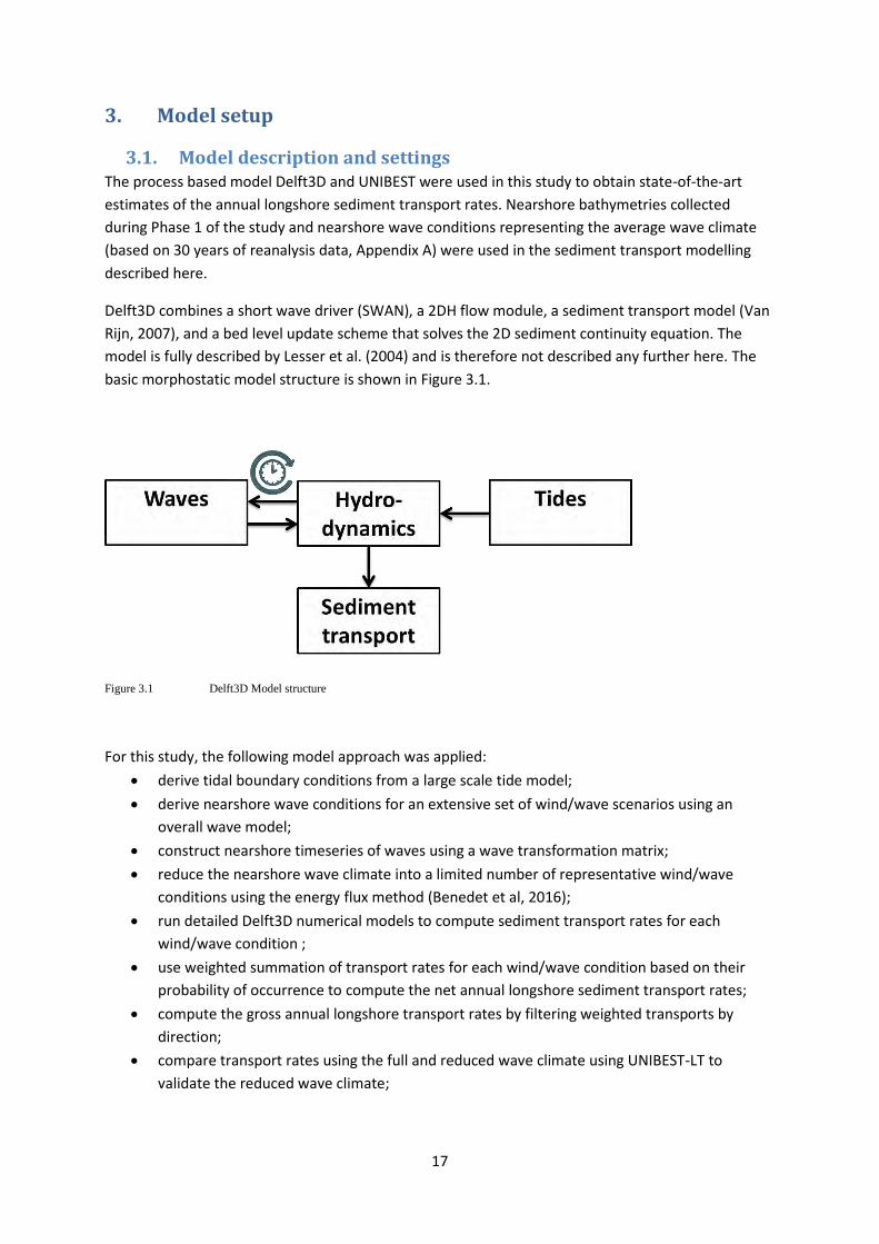
1.4. Approach

The approach followed in this study can be summarized as follows:

• Set-up and apply large-scale wave and hydrodynamic models for northern Sri Lanka using

respectively SWAN and Delft3D.

• Set-up and apply detailed Delft3D numerical models to obtain estimates of longshore sediment

transport at locations of interest

• Provide conclusions and recommendations with respect to the longshore sediment transport

rates and sustainability (siltation) of the proposed harbours and potential negative coastal

impacts that may arise.

1.5. Outline

This chapter describes the background and objectives of the study. In Chapter 2, site descriptions and

data are presented. Chapter 3 describes the model set-up and model results. Finally, Conclusions and

recommendations are given in Chapter 4.

2

2. Site description and data

2.1. Sri Lanka

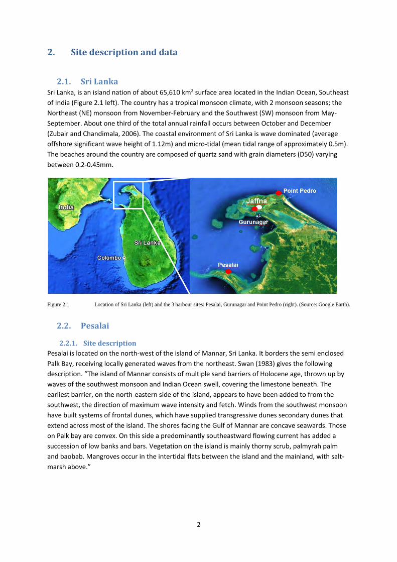
Sri Lanka, is an island nation of about 65,610 km2 surface area located in the Indian Ocean, Southeast

of India (Figure 2.1 left). The country has a tropical monsoon climate, with 2 monsoon seasons; the

Northeast (NE) monsoon from November-February and the Southwest (SW) monsoon from May-

September. About one third of the total annual rainfall occurs between October and December

(Zubair and Chandimala, 2006). The coastal environment of Sri Lanka is wave dominated (average

offshore significant wave height of 1.12m) and micro-tidal (mean tidal range of approximately 0.5m).

The beaches around the country are composed of quartz sand with grain diameters (D50) varying

between 0.2-0.45mm.

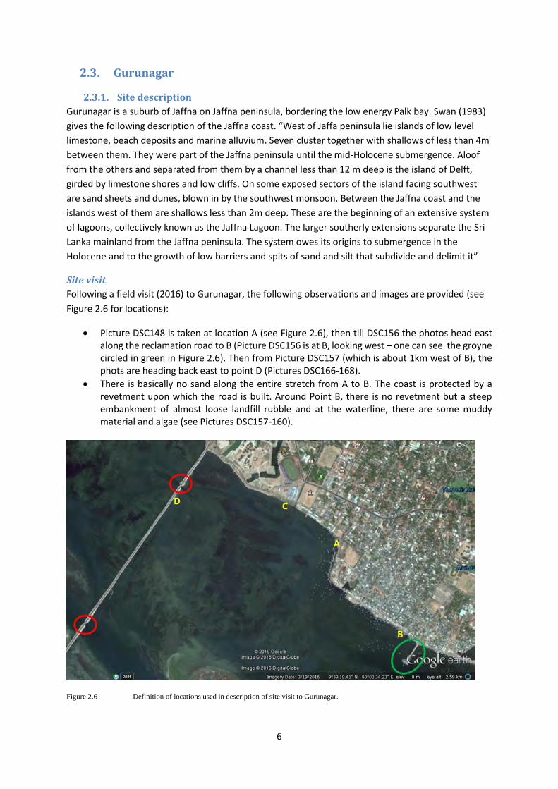
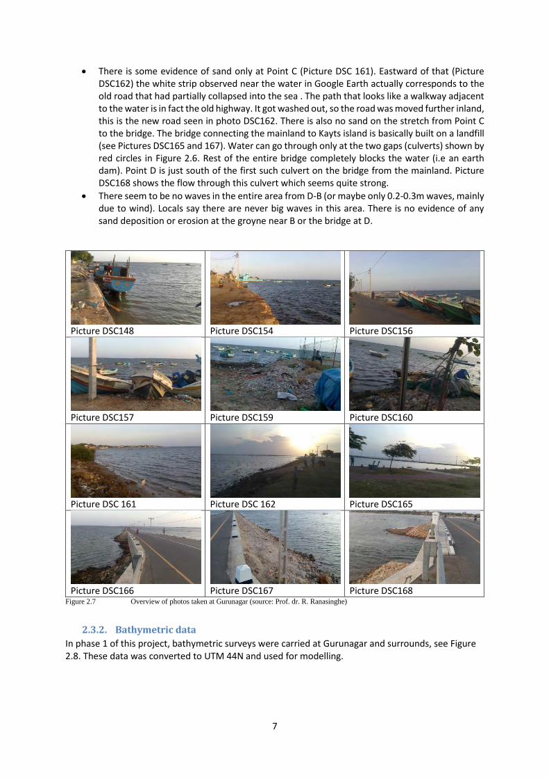
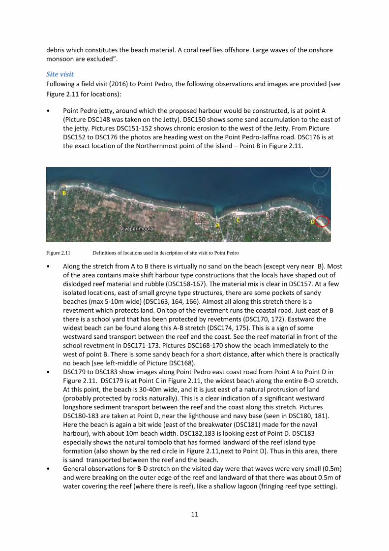
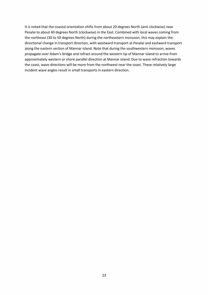
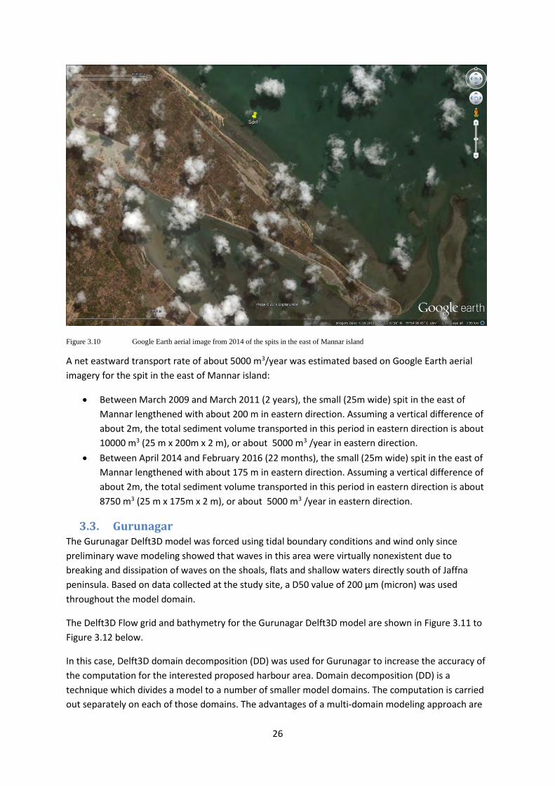
Figure 2.1 Location of Sri Lanka (left) and the 3 harbour sites: Pesalai, Gurunagar and Point Pedro (right). (Source: Google Earth).

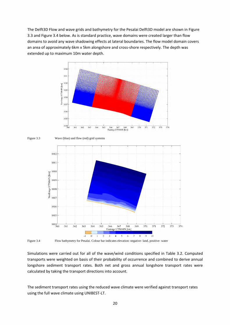
2.2. Pesalai

2.2.1. Site description

Pesalai is located on the north-west of the island of Mannar, Sri Lanka. It borders the semi enclosed

Palk Bay, receiving locally generated waves from the northeast. Swan (1983) gives the following

des riptio . The isla d of Ma ar o sists of ultiple sa d arriers of Holo e e age, thro up waves of the southwest monsoon and Indian Ocean swell, covering the limestone beneath. The

earliest barrier, on the north-eastern side of the island, appears to have been added to from the

southwest, the direction of maximum wave intensity and fetch. Winds from the southwest monsoon

have built systems of frontal dunes, which have supplied transgressive dunes secondary dunes that

extend across most of the island. The shores facing the Gulf of Mannar are concave seawards. Those

on Palk bay are convex. On this side a predominantly southeastward flowing current has added a

succession of low banks and bars. Vegetation on the island is mainly thorny scrub, palmyrah palm

and baobab. Mangroves occur in the intertidal flats between the island and the mainland, with salt-

arsh a o e.

3

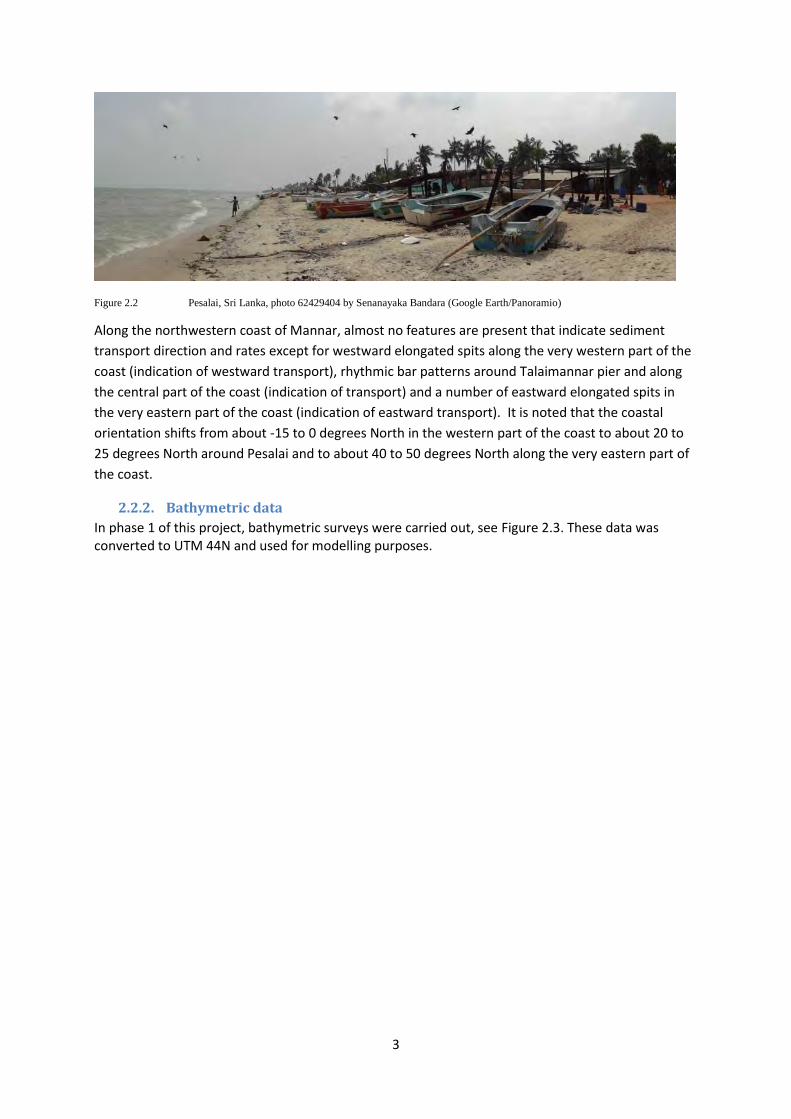
Figure 2.2 Pesalai, Sri Lanka, photo 62429404 by Senanayaka Bandara (Google Earth/Panoramio)

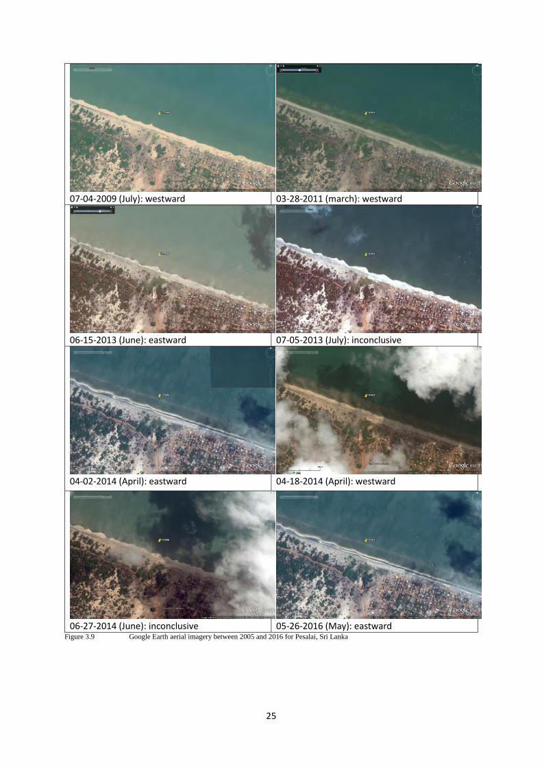
Along the northwestern coast of Mannar, almost no features are present that indicate sediment

transport direction and rates except for westward elongated spits along the very western part of the

coast (indication of westward transport), rhythmic bar patterns around Talaimannar pier and along

the central part of the coast (indication of transport) and a number of eastward elongated spits in

the very eastern part of the coast (indication of eastward transport). It is noted that the coastal

orientation shifts from about -15 to 0 degrees North in the western part of the coast to about 20 to

25 degrees North around Pesalai and to about 40 to 50 degrees North along the very eastern part of

the coast.

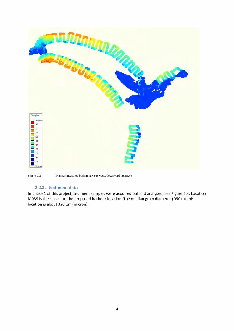
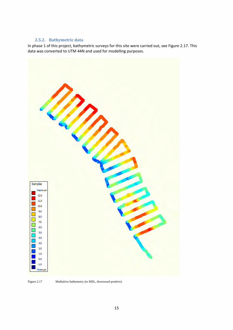
2.2.2. Bathymetric data

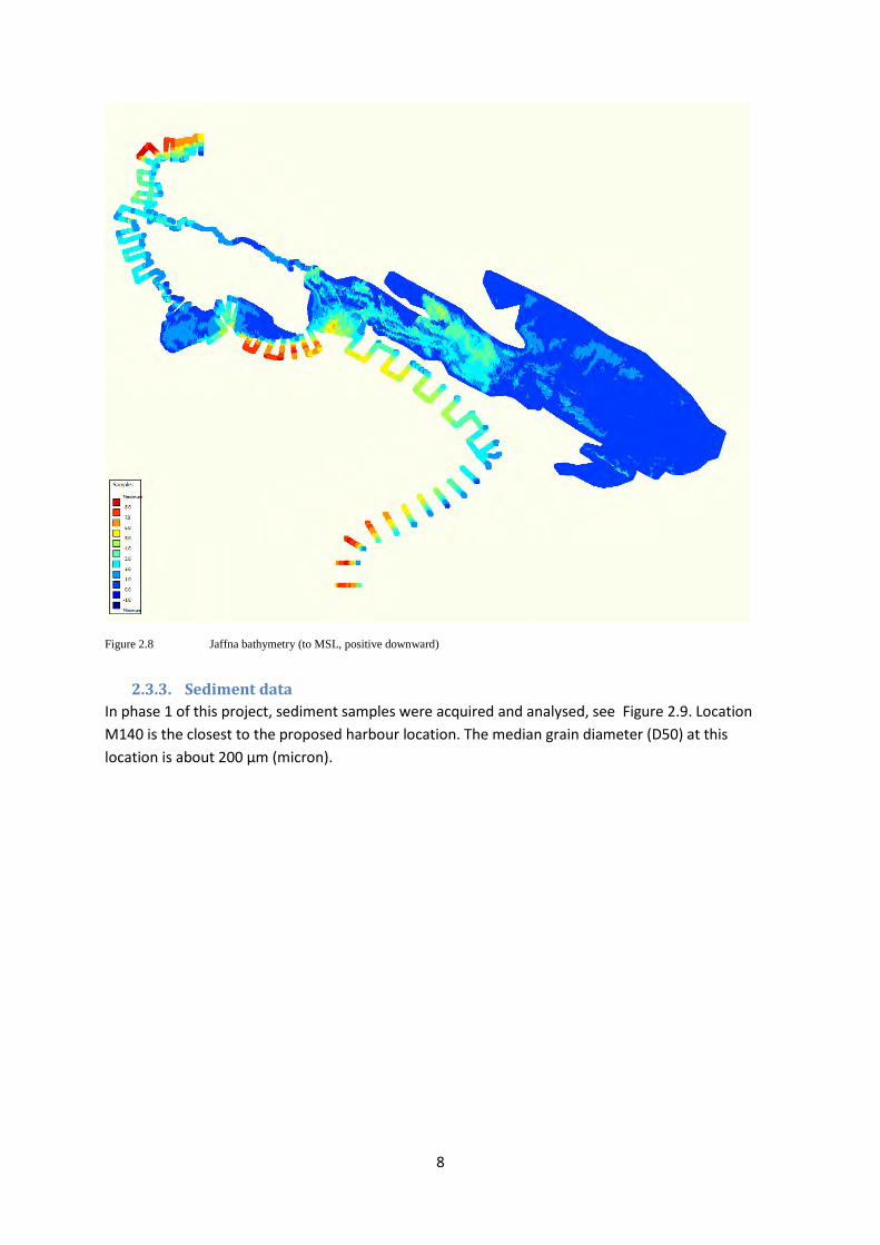
In phase 1 of this project, bathymetric surveys were carried out, see Figure 2.3. These data was

converted to UTM 44N and used for modelling purposes.

4

Figure 2.3 Mannar measured bathymetry (to MSL, downward positive)

2.2.3. Sediment data

In phase 1 of this project, sediment samples were acquired out and analysed, see Figure 2.4. Location

M089 is the closest to the proposed harbour location. The median grain diameter (D50) at this

location is about 320 µm (micron).

5

Figure 2.4 Sieving graph Mannar

2.2.4. Layout

Figure 2.5 shows the proposed fishery harbour layout at Pesalai.

Figure 2.5 Proposed fishery harbour layout at Pesalai by the Department of Civil engineering, University of Moratuwa, Sri Lanka

6

2.3. Gurunagar

2.3.1. Site description

Gurunagar is a suburb of Jaffna on Jaffna peninsula, bordering the low energy Palk bay. Swan (1983)

gives the following description of the Jaffna coast. West of Jaffa peninsula lie islands of low level

limestone, beach deposits and marine alluvium. Seven cluster together with shallows of less than 4m

between them. They were part of the Jaffna peninsula until the mid-Holocene submergence. Aloof

from the others and separated from them by a channel less than 12 m deep is the island of Delft,

girded by limestone shores and low cliffs. On some exposed sectors of the island facing southwest

are sand sheets and dunes, blown in by the southwest monsoon. Between the Jaffna coast and the

islands west of them are shallows less than 2m deep. These are the beginning of an extensive system

of lagoons, collectively known as the Jaffna Lagoon. The larger southerly extensions separate the Sri

Lanka mainland from the Jaffna peninsula. The system owes its origins to submergence in the

Holocene and to the growth of low barriers and spits of sand and silt that su di ide a d deli it it

Site visit

Following a field visit (2016) to Gurunagar, the following observations and images are provided (see

Figure 2.6 for locations):

Picture DSC148 is taken at location A (see Figure 2.6), then till DSC156 the photos head east

along the reclamation road to B (Picture DSC156 is at B, looking west – one can see the groyne

circled in green in Figure 2.6). Then from Picture DSC157 (which is about 1km west of B), the

phots are heading back east to point D (Pictures DSC166-168).

There is basically no sand along the entire stretch from A to B. The coast is protected by a

revetment upon which the road is built. Around Point B, there is no revetment but a steep

embankment of almost loose landfill rubble and at the waterline, there are some muddy

material and algae (see Pictures DSC157-160).

Figure 2.6 Definition of locations used in description of site visit to Gurunagar.

7

There is some evidence of sand only at Point C (Picture DSC 161). Eastward of that (Picture

DSC162) the white strip observed near the water in Google Earth actually corresponds to the

old road that had partially collapsed into the sea . The path that looks like a walkway adjacent

to the water is in fact the old highway. It got washed out, so the road was moved further inland,

this is the new road seen in photo DSC162. There is also no sand on the stretch from Point C

to the bridge. The bridge connecting the mainland to Kayts island is basically built on a landfill

(see Pictures DSC165 and 167). Water can go through only at the two gaps (culverts) shown by

red circles in Figure 2.6. Rest of the entire bridge completely blocks the water (i.e an earth

dam). Point D is just south of the first such culvert on the bridge from the mainland. Picture

DSC168 shows the flow through this culvert which seems quite strong.

There seem to be no waves in the entire area from D-B (or maybe only 0.2-0.3m waves, mainly

due to wind). Locals say there are never big waves in this area. There is no evidence of any

sand deposition or erosion at the groyne near B or the bridge at D.

Picture DSC148

Picture DSC154

Picture DSC156

Picture DSC157

Picture DSC159

Picture DSC160

Picture DSC 161

Picture DSC 162

Picture DSC165

Picture DSC166

Picture DSC167

Picture DSC168

Figure 2.7 Overview of photos taken at Gurunagar (source: Prof. dr. R. Ranasinghe)

2.3.2. Bathymetric data

In phase 1 of this project, bathymetric surveys were carried at Gurunagar and surrounds, see Figure

2.8. These data was converted to UTM 44N and used for modelling.

8

Figure 2.8 Jaffna bathymetry (to MSL, positive downward)

2.3.3. Sediment data

In phase 1 of this project, sediment samples were acquired and analysed, see Figure 2.9. Location

M140 is the closest to the proposed harbour location. The median grain diameter (D50) at this

location is about 200 µm (micron).

9

Figure 2.9 Sieving graph Jaffna

2.3.4. Layout

Figure 2.10 shows the conceptual design for the proposed fishery harbour at Gurunagar, Jaffna. Note

that besides the location of the breakwaters, the outline of the entrance channel to be dredged is

also presented herein.

10

Figure 2.10 Conceptual design for proposed fishery harbour at Gurunagar by Power Asia (Pvt.) Ltd., Sri Lanka.

2.4. Point Pedro

2.4.1. Site description

Point Pedro is located in Jaffna District, at the northernmost point of Sri Lanka. Swan (1983) gives the

following description. This stret h of oast o upies the orther fla k of the Jaff a pe i sula. It

faces seas that are less than 13m deep and for this reason is not affected by medium and long period

ocean swell. The coast is low lying and composed of corallian limestone, capped with red calcic

laptosols which are weathered beach and Aeolian deposits. Raised Holocene deposits lie within 3m

of the high water mark. The coastline is devoid of indentations, excepting for the inlet of

Thondaimannar lagoon. In plan, it is multi-convex and without prominent headlands. The coast is

undergoing slow retreat. Cut back, mainly during the north-east monsoon, has produced low cliffs

and caves in places and an extensive inter-tidal shore platform, veneered with coarse calcareous

11

debris which constitutes the beach material. A coral reef lies offshore. Large waves of the onshore

monsoon are excluded .

Site visit

Following a field visit (2016) to Point Pedro, the following observations and images are provided (see

Figure 2.11 for locations):

• Point Pedro jetty, around which the proposed harbour would be constructed, is at point A

(Picture DSC148 was taken on the Jetty). DSC150 shows some sand accumulation to the east of

the jetty. Pictures DSC151-152 shows chronic erosion to the west of the Jetty. From Picture

DSC152 to DSC176 the photos are heading west on the Point Pedro-Jaffna road. DSC176 is at

the exact location of the Northernmost point of the island – Point B in Figure 2.11.

Figure 2.11 Definitions of locations used in description of site visit to Point Pedro

• Along the stretch from A to B there is virtually no sand on the beach (except very near B). Most

of the area contains make shift harbour type constructions that the locals have shaped out of

dislodged reef material and rubble (DSC158-167). The material mix is clear in DSC157. At a few

isolated locations, east of small groyne type structures, there are some pockets of sandy

beaches (max 5-10m wide) (DSC163, 164, 166). Almost all along this stretch there is a

revetment which protects land. On top of the revetment runs the coastal road. Just east of B

there is a school yard that has been protected by revetments (DSC170, 172). Eastward the

widest beach can be found along this A-B stretch (DSC174, 175). This is a sign of some

westward sand transport between the reef and the coast. See the reef material in front of the

school revetment in DSC171-173. Pictures DSC168-170 show the beach immediately to the

west of point B. There is some sandy beach for a short distance, after which there is practically

no beach (see left-middle of Picture DSC168).

• DSC179 to DSC183 show images along Point Pedro east coast road from Point A to Point D in

Figure 2.11. DSC179 is at Point C in Figure 2.11, the widest beach along the entire B-D stretch.

At this point, the beach is 30-40m wide, and it is just east of a natural protrusion of land

(probably protected by rocks naturally). This is a clear indication of a significant westward

longshore sediment transport between the reef and the coast along this stretch. Pictures

DSC180-183 are taken at Point D, near the lighthouse and navy base (seen in DSC180, 181).

Here the beach is again a bit wide (east of the breakwater (DSC181) made for the naval

harbour), with about 10m beach width. DSC182,183 is looking east of Point D. DSC183

especially shows the natural tombolo that has formed landward of the reef island type

formation (also shown by the red circle in Figure 2.11,next to Point D). Thus in this area, there

is sand transported between the reef and the beach.

• General observations for B-D stretch on the visited day were that waves were very small (0.5m)

and were breaking on the outer edge of the reef and landward of that there was about 0.5m of

water covering the reef (where there is reef), like a shallow lagoon (fringing reef type setting).

12

Strong currents are not expected in this area between reef front and coastline. In the channels

between the reef sections, there is fairly strong flows (0.5-0.7m/s). Sand is fine.

Picture DSC148

Picture DSC150

Picture DSC151

Picture DSC152

Picture DSC154

Picture DSC157

Picture DSC158

Picture DSC168

Picture DSC176

Picture DSC179

Picture DSC181

Picture DSC183

Figure 2.12 Overview of photos taken at Point Pedro (Source: Prof. dr. R. Ranasinghe)

2.4.2. Bathymetric data

In phase 1 of this project, bathymetric surveys for this site were carried out, see Figure 2.13. This

data was converted to UTM 44N and used for modelling purposes.

13

Figure 2.13 Point Pedro bathymetry (to MSL, downward positive)

2.4.3. Sediment data

In phase 1 of this project, sediment samples were acquired and analysed, see Figure 2.14.

Figure 2.14 Sieving graph of Point Pedro (National building research organization, Colombo, Sri Lanka)

2.4.4. Layout

Figure 2.15 shows the proposed fishery harbour layout at Point Pedro.

14

Figure 2.15 Proposed fishery harbour at Point Pedro by the department of Civil engineering, University of Moratuwa, Sri Lanka

2.5. Mullaitivu

2.5.1. Site description

Mullaitivu is situated on the north-eastern coast of Northern Province, Sri Lanka. Swan (1983) gives

the following description. The coast between Nayaru and Peparaputti is low and sandy, with

evidence of abundant progradation. This is particularly active at Mullaitivu, where large offshore

banks of sand have been laid down. Recent beach and dune sands occupy a broad swath behind the

shoreline. West of those and parallel to them are long lagoons. Beyond them are watered laptosols.

Figure 2.16 Mullaitivu thuraimugam, photo 10900317 by Sivam Kandar (Google Earth/Panoramio),

15

2.5.2. Bathymetric data

In phase 1 of this project, bathymetric surveys for this site were carried out, see Figure 2.17. This

data was converted to UTM 44N and used for modelling purposes.

Figure 2.17 Mullaitivu bathymetry (to MSL, downward positive).

16

2.5.3. Sediment data

In phase 1 of this project, sediment samples were acquired and analysed, see Figure 2.18.

Figure 2.18 Sieving graph Mullaitivu.

2.5.4. Layout

The proposed harbour at Mullaitivu was abandoned during the course of this study.

2.6. Wave data

As a follow up to and improvement on ERA-40, The European centre for medium range weather

forecast (ECMWF) has produced a global wind and wave reanalysis dataset with a resolution of 1ºx1º

from January 1979 and on-going. (0.75º x 0.75º resolution if downloaded from the ECMWF website

http://dataportal.ecmwf.int/data/d/interim_daily, free for research and commercial proposes). The

wave model used in the reanalysis is the third generation WAM model, which is coupled with the

atmospheric model. The quality of the ERA-interim wind and offshore wave data is high, even higher

than that of the ECMWF operational model for data up to 2005. The wave data are not valid

nearshore because the used WAM model contains on limited shallow water wave physics and the

representation of the coastlines is very coarse.

.000%

10.000%

20.000%

30.000%

40.000%

50.000%

60.000%

70.000%

80.000%

90.000%

100.000%

10 100 1000 10000

cum

ula

tiv

e w

eig

ht

(%)

Particle size (mu)

Mullaitivu sieving curve

M95

M142

AVERAGE

17

3. Model setup

3.1. Model description and settings

The process based model Delft3D and UNIBEST were used in this study to obtain state-of-the-art

estimates of the annual longshore sediment transport rates. Nearshore bathymetries collected

during Phase 1 of the study and nearshore wave conditions representing the average wave climate

(based on 30 years of reanalysis data, Appendix A) were used in the sediment transport modelling

described here.

Delft3D combines a short wave driver (SWAN), a 2DH flow module, a sediment transport model (Van

Rijn, 2007), and a bed level update scheme that solves the 2D sediment continuity equation. The

model is fully described by Lesser et al. (2004) and is therefore not described any further here. The

basic morphostatic model structure is shown in Figure 3.1.

Figure 3.1 Delft3D Model structure

For this study, the following model approach was applied:

derive tidal boundary conditions from a large scale tide model;

derive nearshore wave conditions for an extensive set of wind/wave scenarios using an

overall wave model;

construct nearshore timeseries of waves using a wave transformation matrix;

reduce the nearshore wave climate into a limited number of representative wind/wave

conditions using the energy flux method (Benedet et al, 2016);

run detailed Delft3D numerical models to compute sediment transport rates for each

wind/wave condition ;

use weighted summation of transport rates for each wind/wave condition based on their

probability of occurrence to compute the net annual longshore sediment transport rates;

compute the gross annual longshore transport rates by filtering weighted transports by

direction;

compare transport rates using the full and reduced wave climate using UNIBEST-LT to

validate the reduced wave climate;

18

Model forcings applied included tide, waves and local winds (except for Gurunagar where waves

were not included due to absence of significant waves in the area). Wave conditions were derived

from a series of nested SWAN wave models forced with ERA-interim (Dee et al., 2011) wave and wind

data (Appendix A). Following standard practice to reduce computational times of numerical flow-

wave coupled sediment transport models, the full wave climate was reduced to 18 representative

wave and wind conditions (6 wave directional classes and 3 wave height classes) using the energy-

flux method (Benedet et al., 2016; Appendix A). Tidal boundary conditions were derived from an

overall tidal model of Northern Sri Lanka that was forced using Global Inverse Tide Model TPXO 7.2

(Appendix B).

Delft3D parameter settings closely followed those that were successfully used in a comprehensive

modeling study undertaken for the South West coast of Sri Lanka (Duong, 2015) and are summarized

in Table 3.1 below.

Table 3.1 Model parameter settings.

Parameter Adopted value

Hydrodynamic time step (s) 3

Hydrodynamic spin-up time (hrs) 24

Horizontal eddy viscosity (m2/s) 1

Horizontal eddy diffusivity (m2/s) 1

Chezy bottom friction coefficient (m1/2/s)* 65

Directional wave spreading (deg) 25o

Sediment transport formula Van Rijn (2007)

Dry cell erosion factor 0.5

Wave-flow coupling time (min) 30

Output interval for whole domain (min) 30

Output interval for pre-defined observation points and

cross-sections (min)

10

Boundary Conditions Water Level (Astronomic) and Neumann

* in the reef areas of the Point Pedro site, a Chezy coefficient of 35(m1/2/s) was used to represent the higher friction in reef

areas.

3.2. Pesalai

Wave and wind conditions used in the Pesalai Delft3D model are shown in Table 3.2 below. The

westerly wave conditions were not taken into account in this reduced climate as preliminary

simulations showed that these conditions resulted in high angle incident wave near the coast and

very small to negligible transports. These high wave angle conditions may however have a significant

impact on the plan form morphology of the Pesalai coast (Ashton and Murray, 2006). Based on data

collected at the study site, a D50 value of 320 µm (micron) was used throughout the model domain.

For Pesalai, tidal boundary conditions (Neumann conditions for lateral boundaries and water levels

for sea boundary, see Figure 3.2) were applied by nesting the local model in the large scale tidal

model for Northern Sri Lanka (Appendix B). For each wave condition, the model was run for the

period 18 January 2015 18h35m to 20 January 2015 19h25m using a spin up time of 24hrs.

19

Figure 3.2 Water level boundary conditions applied (red) in the Pesalai model

Table 3.2 Wave and wind forcings: 18 reduced wave and wind conditions

Wi Hs

(m)

Tp

(s)

Dir

(o)

Duration

Di (days)

Weight

Pi

Speed

(m/s)

Direction

(o)

W00 - - - 230.07 0.630 - -

W01 0.33 3.23 323.15 12.05 0.033 2.50 14.14

W02 0.67 3.22 324.47 2.96 0.008 5.02 13.20

W03 0.95 3.66 316.95 1.12 0.003 8.11 10.20

W04 0.41 2.80 0.87 9.07 0.025 5.67 30.36

W05 0.67 3.14 4.37 2.99 0.008 8.01 26.32

W06 0.80 3.42 358.03 1.83 0.005 8.84 28.40

W07 0.42 2.65 19.47 9.41 0.026 6.14 36.74

W08 0.62 2.99 19.07 4.18 0.011 8.11 34.84

W09 0.72 3.20 18.63 2.49 0.007 8.71 38.05

W10 0.38 2.42 29.89 12.72 0.035 5.82 41.74

W11 0.57 2.87 29.76 4.76 0.013 7.72 40.96

W12 0.68 3.08 29.26 3.04 0.008 8.41 41.22

W13 0.36 2.36 38.66 15.79 0.043 5.50 47.90

W14 0.55 2.79 38.42 5.48 0.015 7.37 46.25

W15 0.64 2.98 38.03 3.47 0.010 8.04 46.85

W16 0.24 2.06 58.60 30.38 0.083 4.16 67.18

W17 0.42 2.49 53.72 8.98 0.025 6.15 57.82

W18 0.54 2.75 48.95 4.46 0.012 7.04 53.01

20

The Delft3D Flow and wave grids and bathymetry for the Pesalai Delft3D model are shown in Figure

3.3 and Figure 3.4 below. As is standard practice, wave domains were created larger than flow

domains to avoid any wave shadowing effects at lateral boundaries. The flow model domain covers

an area of approximately 6km x 5km alongshore and cross-shore respectively. The depth was

extended up to maximum 10m water depth.

Figure 3.3 Wave (blue) and flow (red) grid systems

Figure 3.4 Flow bathymetry for Pesalai. Colour bar indicates elevation: negative- land, positive- water

Simulations were carried out for all of the wave/wind conditions specified in Table 3.2. Computed

transports were weighted on basis of their probability of occurrence and combined to derive annual

longshore sediment transport rates. Both net and gross annual longshore transport rates were

calculated by taking the transport directions into account.

The sediment transport rates using the reduced wave climate were verified against transport rates

using the full wave climate using UNIBEST-LT.

21

3.2.1. Results

Sediment transport rates obtained for wave condition w15 which produced the highest sediment

transport at this location are illustrated in Figure 3.5 below.

Figure 3.5 Highest sediment transport from wave condition w15. Top figure – whole transport field; Bottom figures – Zoom in:

Green box – Left part, Red box – Middle part, Black box – Right part. Black arrows are sediment transport vectors. Colour bar indicates

elevation: negative – land, positive – water.

The total annual net alongshore sediment transport rate (LST) at Pesalai is about 10,000 m3/year to

the west. Gross transport rates are 11,000 m3/year to the West and 1,000 m3/year to the East. The

sediment budget at Pesalai is shown in Figure 3.6 below.

22

Figure 3.6 Sediment budget at Pesalai – white arrows, unit – 1000m3/year. White dashed lines represent the proposed harbour

breakwaters which were not included in the model.

It is generally believed that the net alongshore transport direction along Mannar is from west to east.

While this seems to be true for both the western (Talaimannar Pier) and eastern (spits) sections of

Mannar island. Plan form shapes and bar patterns at times indicate westward transports, both in the

western section (Talaimannar Pier) and central part of Mannar (Pesalai), see Google Earth aerial

imagery in Figure 3.7 to 3.10.

Figure 3.7 Google Earth aerial image of Mannar island, Sri Lanka. Talaimannar Pier in the west, Pesalai in the middle and the

Spit(s) in the East are indicated with markers.

23

It is noted that the coastal orientation shifts from about 20 degrees North (anti clockwise) near

Pesalai to about 40 degrees North (clockwise) in the East. Combined with local waves coming from

the northeast (30 to 50 degrees North) during the northeastern monsoon, this may explain the

directional change in transport direction, with westward transport at Pesalai and eastward transport

along the eastern section of Mannar island. Note that during the southwestern monsoon, waves

propagate o er Ada s ridge a d refract around the western tip of Mannar island to arrive from

approximately western or shore parallel direction at Mannar island. Due to wave refraction towards

the coast, wave directions will be more from the northwest near the coast. These relatively large

incident wave angles result in small transports in eastern direction.

24

09-29-2005 (September): eastward 04-25-2008 (April): westward

05-03-2008 (May): inconclusive 07-04-2009 (July): inconclusive

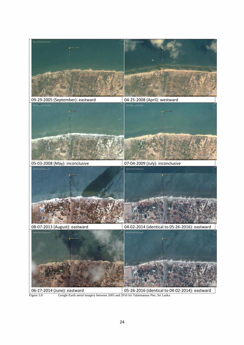
08-07-2013 (August): eastward 04-02-2014 (identical to 05-26-2016): eastward

06-27-2014 (June): eastward 05-26-2016 (identical to 04-02-2014): eastward Figure 3.8 Google Earth aerial imagery between 2005 and 2016 for Talaimannar Pier, Sri Lanka

25

07-04-2009 (July): westward 03-28-2011 (march): westward

06-15-2013 (June): eastward 07-05-2013 (July): inconclusive

04-02-2014 (April): eastward 04-18-2014 (April): westward

06-27-2014 (June): inconclusive 05-26-2016 (May): eastward Figure 3.9 Google Earth aerial imagery between 2005 and 2016 for Pesalai, Sri Lanka

26

Figure 3.10 Google Earth aerial image from 2014 of the spits in the east of Mannar island

A net eastward transport rate of about 5000 m3/year was estimated based on Google Earth aerial

imagery for the spit in the east of Mannar island:

Between March 2009 and March 2011 (2 years), the small (25m wide) spit in the east of

Mannar lengthened with about 200 m in eastern direction. Assuming a vertical difference of

about 2m, the total sediment volume transported in this period in eastern direction is about

10000 m3 (25 m x 200m x 2 m), or about 5000 m3 /year in eastern direction.

Between April 2014 and February 2016 (22 months), the small (25m wide) spit in the east of

Mannar lengthened with about 175 m in eastern direction. Assuming a vertical difference of

about 2m, the total sediment volume transported in this period in eastern direction is about

8750 m3 (25 m x 175m x 2 m), or about 5000 m3 /year in eastern direction.

3.3. Gurunagar

The Gurunagar Delft3D model was forced using tidal boundary conditions and wind only since

preliminary wave modeling showed that waves in this area were virtually nonexistent due to

breaking and dissipation of waves on the shoals, flats and shallow waters directly south of Jaffna

peninsula. Based on data collected at the study site, a D50 value of 200 µm (micron) was used

throughout the model domain.

The Delft3D Flow grid and bathymetry for the Gurunagar Delft3D model are shown in Figure 3.11 to

Figure 3.12 below.

In this case, Delft3D domain decomposition (DD) was used for Gurunagar to increase the accuracy of

the computation for the interested proposed harbour area. Domain decomposition (DD) is a

technique which divides a model to a number of smaller model domains. The computation is carried

out separately on each of those domains. The advantages of a multi-domain modeling approach are

27

the possibility of coupling different models, increase the accuracy of the model in the area of

interest, and increase the modelling efficiency by a parallel execution of the computations on

different domains. Domain decomposition allows for local grid refinement, both in the horizontal

direction and in the vertical direction. The 'Domain Decomposition' toolbox is only available for

Delft3D-FLOW.

The Gurunagar model included lagoons on both sides of the proposed harbour location (as in Figure

3.11), the harbour area is within the blue part in figure 3.11. The sea part of the local model is up to

about 8m depth. Two gaps or culverts, under the landfill bridge connecting the mainland to Kayts

island to the left of the harbour location, where water can go through, were included in the model.

Figure 3.11 Grid system for Gurunagar – Top figure. Domain decomposition – Bottom figures. Black lines are land boundary lines.

28

Figure 3.12 Flow bathymetry for Gurunagar. Top figure - Whole domain. Bottom figures – Zoom in of the bed level of grid

refinement for Gurunagar site. Black lines are land boundary lines. Colour bar indicates elevation: negative – land, positive-water.

3.3.1. Results

Since waves were found to be insignificant here, the model was run for 1 month during the

southwest monsoon period (9 juli 2015 20:00hrs to 10 august 2015 20:00hrs, 1 day spinup, see

Figure 3.13), taking into account tides and temporally and spatially varying air pressure and wind

fields. Net sediment transport rates near the proposed harbor location are shown in Figure 3.14. As

can be seen from this figure, sediment transport rates in this area are generally very small, except

near the location of two gaps under the landfill bridge.

29

Figure 3.13 Water level boundary conditions applied in the Gurunagar model

Figure 3.14 Residual sediment transport at harbour site: Red arrows. Colour bar shows elevation: negative – land, positive – water.

The total annual net and gross sediment transport rates at Gurunagar are the same and about 5,000

m3/year from West to East. The sediment budget at Gurunagar is shown in Figure 3.15 below.

30

Figure 3.15 Sediment budget at Gurunagar - white arrows, unit 1000 m3/year. White dashed lines represent the proposed harbour

breakwaters which were not included in the model

3.4. Point Pedro

Wave and wind conditions used in the Point Pedro Delft3D model are shown in Table 3.3 below.

Based on data collected at the study site, a D50 value of 430 µm (micron) was used in all non-reef

sandy areas of the model domain. For each wave condition, the model was run for 1 day.

Table 3.3 Wave and wind forcings: 18 reduced wave and wind conditions

Wi Hs

(m)

Tp

(s)

Dir

(o)

Duration

Di (days)

Weight

Pi

Speed

(m/s)

Direction

(o)

W00 - - - 224 0.6147 - -

W01 0.49 4.93 332 0.26 0.0007 6.32 259.17

W02 0.74 5.23 322 0.11 0.0003 7.18 260.02

W03 1.01 5.37 304 0.06 0.0002 10.98 261.79

W04 0.82 6.64 43 7.51 0.0206 3.84 19.98

W05 1.14 7.18 44 3.59 0.0098 6.26 25.52

W06 1.58 8.09 40 1.60 0.0044 5.99 14.04

W07 0.73 6.34 54 14.72 0.0403 6.56 37.87

W08 0.99 6.74 53 7.57 0.0207 8.16 36.68

W09 1.30 7.34 53 3.51 0.0096 8.53 31.81

W10 0.68 6.30 58 16.17 0.0443 6.01 39.67

W11 0.93 6.72 58 8.24 0.0226 7.62 37.85

W12 1.25 7.26 58 4.06 0.0111 8.75 33.92

W13 0.66 6.44 64 15.42 0.0423 5.57 40.07

W14 0.95 6.79 65 7.08 0.0194 8.11 35.89

W15 1.27 7.37 65 3.58 0.0098 9.05 33.49

W16 0.47 6.18 78 30.72 0.0842 2.74 47.45

W17 0.71 6.63 73 12.24 0.0335 4.65 43.01

W18 1.11 7.08 70 4.56 0.0125 7.82 35.91

31

The Delft3D Flow and wave grids and bathymetry for the Point Pedro Delft3D model are shown in

Figure 3.16 and Figure 3.17 below. As is standard practice, wave domains were created larger than

flow domains to avoid any wave shadowing effects at lateral boundaries. The flow model domain of

Point Pedro covers about 2km alongshore each side of the proposed harbour location and the

offshore area was extended up to maximum 15m water depth.

Figure 3.16 Wave (blue) and flow (red) grid systems

Figure 3.17 Flow Bathymetry: whole flow domain (left figure) and zoom-in of the proposed harbour location area (in red box, right

figure). Colour bar indicates elevation: negative – land, positive – water.

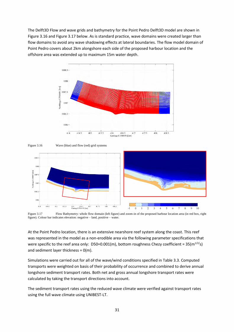
At the Point Pedro location, there is an extensive nearshore reef system along the coast. This reef

was represented in the model as a non-erodible area via the following parameter specifications that

were specific to the reef area only: D50=0.001(m), bottom roughness Chezy coefficient = 35(m1/2/s)

and sediment layer thickness = 0(m).

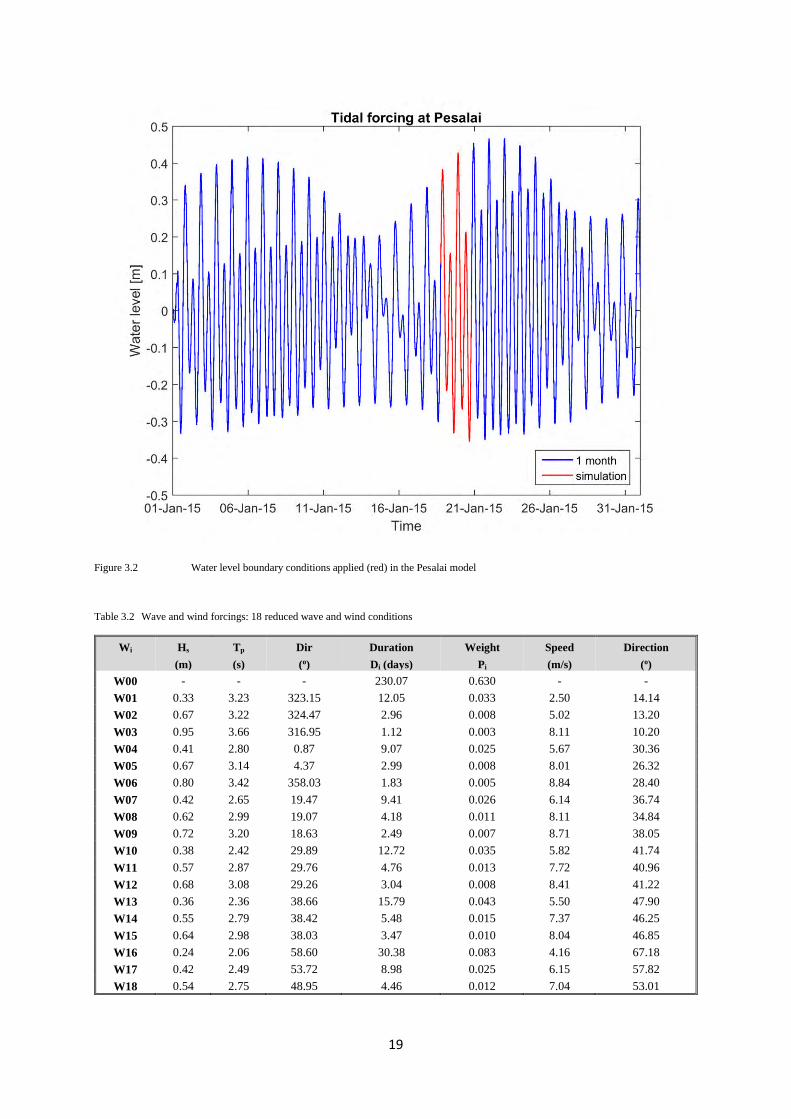
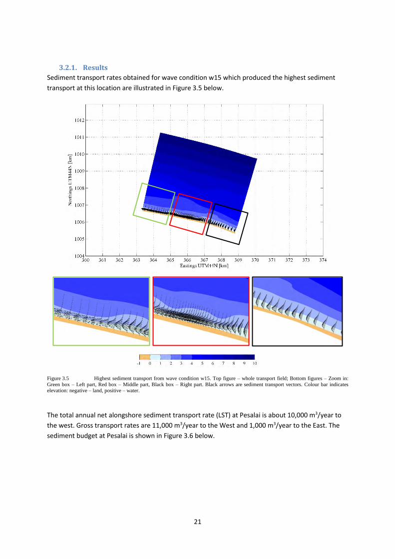
Simulations were carried out for all of the wave/wind conditions specified in Table 3.3. Computed

transports were weighted on basis of their probability of occurrence and combined to derive annual

longshore sediment transport rates. Both net and gross annual longshore transport rates were

calculated by taking the transport directions into account.

The sediment transport rates using the reduced wave climate were verified against transport rates

using the full wave climate using UNIBEST-LT.

32

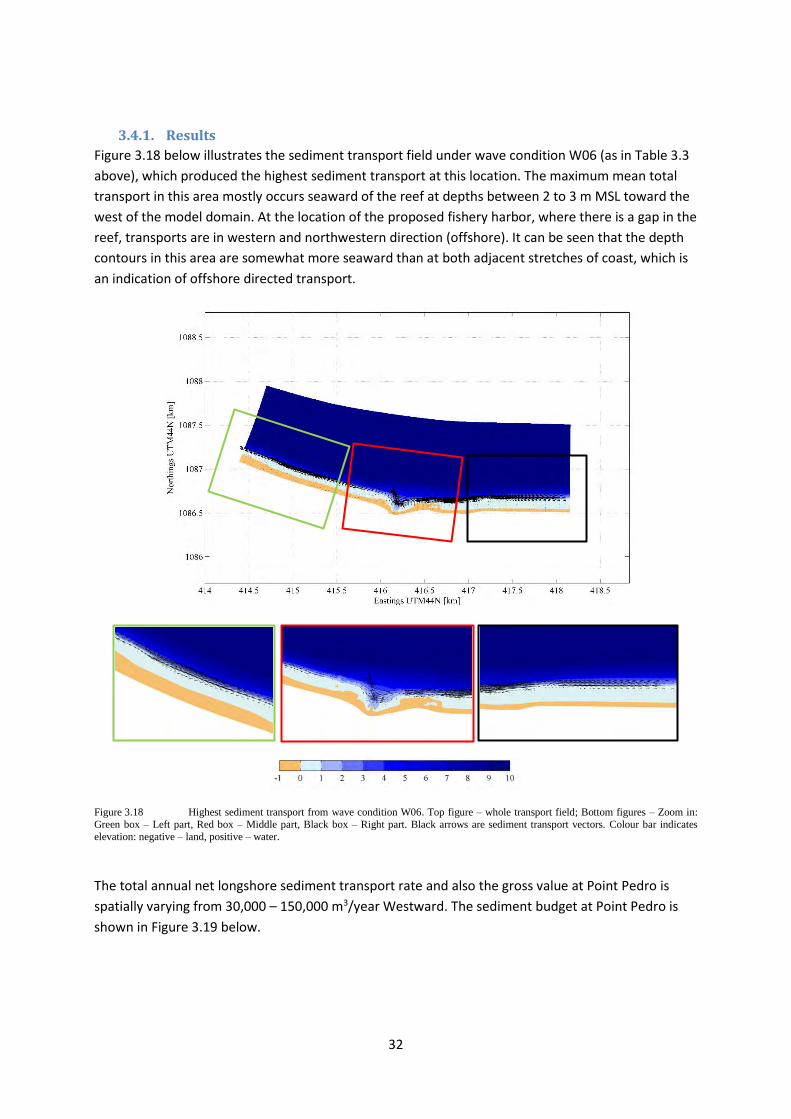
3.4.1. Results

Figure 3.18 below illustrates the sediment transport field under wave condition W06 (as in Table 3.3

above), which produced the highest sediment transport at this location. The maximum mean total

transport in this area mostly occurs seaward of the reef at depths between 2 to 3 m MSL toward the

west of the model domain. At the location of the proposed fishery harbor, where there is a gap in the

reef, transports are in western and northwestern direction (offshore). It can be seen that the depth

contours in this area are somewhat more seaward than at both adjacent stretches of coast, which is

an indication of offshore directed transport.

Figure 3.18 Highest sediment transport from wave condition W06. Top figure – whole transport field; Bottom figures – Zoom in:

Green box – Left part, Red box – Middle part, Black box – Right part. Black arrows are sediment transport vectors. Colour bar indicates

elevation: negative – land, positive – water.

The total annual net longshore sediment transport rate and also the gross value at Point Pedro is

spatially varying from 30,000 – 150,000 m3/year Westward. The sediment budget at Point Pedro is

shown in Figure 3.19 below.

33

Figure 3.19 Sediment budget at Point Pedro: unit – 1000m3/year, white arrows – sediment transports behind the reefs, blue arrows –

sediment transport between the reefs and the beach, white dashed lines represent the proposed harbour breakwaters which were not included

in the model.

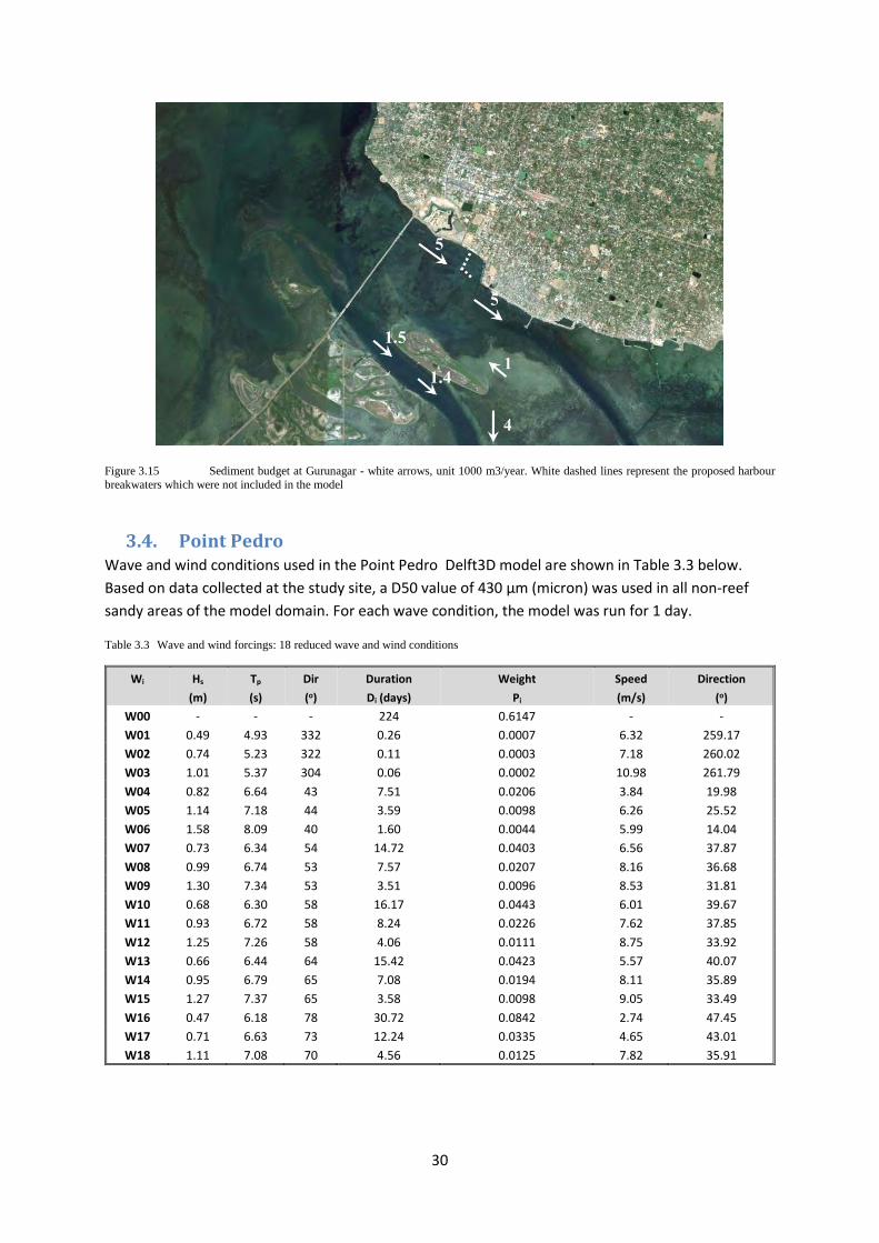
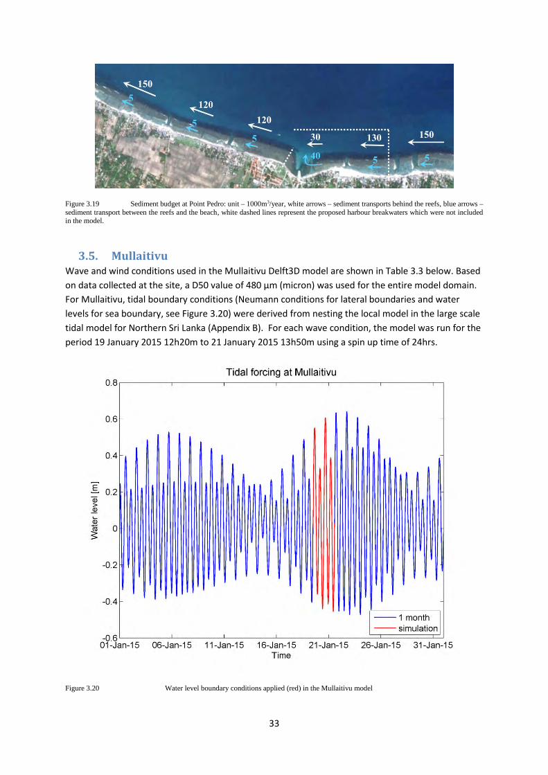
3.5. Mullaitivu

Wave and wind conditions used in the Mullaitivu Delft3D model are shown in Table 3.3 below. Based

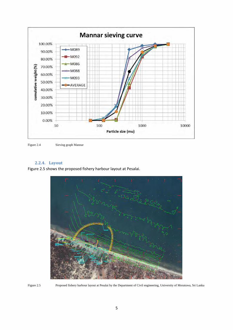
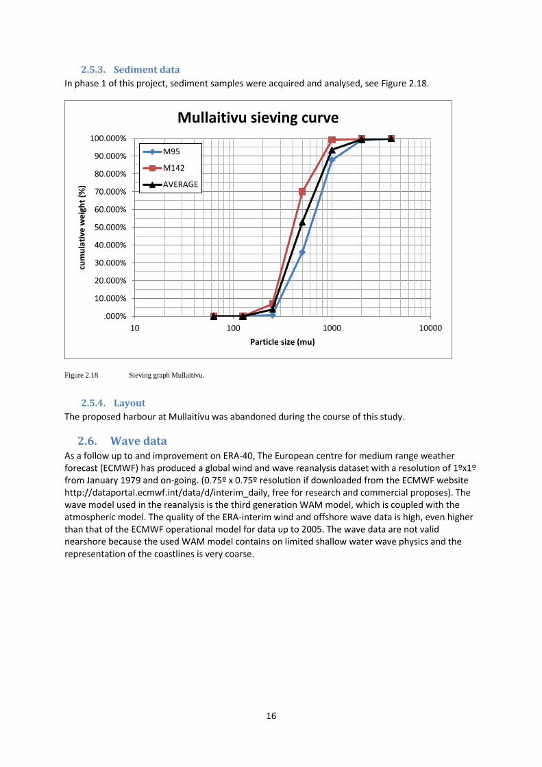
on data collected at the site, a D50 value of 480 µm (micron) was used for the entire model domain.

For Mullaitivu, tidal boundary conditions (Neumann conditions for lateral boundaries and water

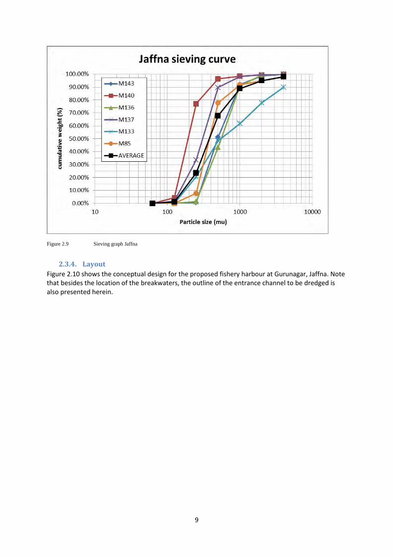
levels for sea boundary, see Figure 3.20) were derived from nesting the local model in the large scale

tidal model for Northern Sri Lanka (Appendix B). For each wave condition, the model was run for the

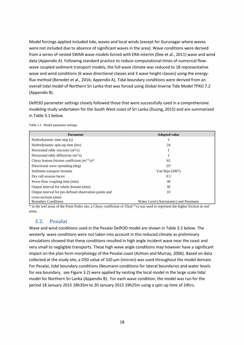
period 19 January 2015 12h20m to 21 January 2015 13h50m using a spin up time of 24hrs.

Figure 3.20 Water level boundary conditions applied (red) in the Mullaitivu model

34

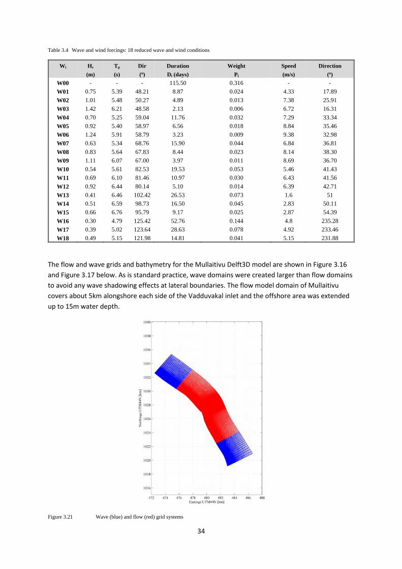
Table 3.4 Wave and wind forcings: 18 reduced wave and wind conditions

Wi Hs

(m)

Tp

(s)

Dir

(o)

Duration

Di (days)

Weight

Pi

Speed

(m/s)

Direction

(o)

W00 - - - 115.50 0.316 - -

W01 0.75 5.39 48.21 8.87 0.024 4.33 17.89

W02 1.01 5.48 50.27 4.89 0.013 7.38 25.91

W03 1.42 6.21 48.58 2.13 0.006 6.72 16.31

W04 0.70 5.25 59.04 11.76 0.032 7.29 33.34

W05 0.92 5.40 58.97 6.56 0.018 8.84 35.46

W06 1.24 5.91 58.79 3.23 0.009 9.38 32.98

W07 0.63 5.34 68.76 15.90 0.044 6.84 36.81

W08 0.83 5.64 67.83 8.44 0.023 8.14 38.30

W09 1.11 6.07 67.00 3.97 0.011 8.69 36.70

W10 0.54 5.61 82.53 19.53 0.053 5.46 41.43

W11 0.69 6.10 81.46 10.97 0.030 6.43 41.56

W12 0.92 6.44 80.14 5.10 0.014 6.39 42.71

W13 0.41 6.46 102.42 26.53 0.073 1.6 51

W14 0.51 6.59 98.73 16.50 0.045 2.83 50.11

W15 0.66 6.76 95.79 9.17 0.025 2.87 54.39

W16 0.30 4.79 125.42 52.76 0.144 4.8 235.28

W17 0.39 5.02 123.64 28.63 0.078 4.92 233.46

W18 0.49 5.15 121.98 14.81 0.041 5.15 231.88

The flow and wave grids and bathymetry for the Mullaitivu Delft3D model are shown in Figure 3.16

and Figure 3.17 below. As is standard practice, wave domains were created larger than flow domains

to avoid any wave shadowing effects at lateral boundaries. The flow model domain of Mullaitivu

covers about 5km alongshore each side of the Vadduvakal inlet and the offshore area was extended

up to 15m water depth.

Figure 3.21 Wave (blue) and flow (red) grid systems

35

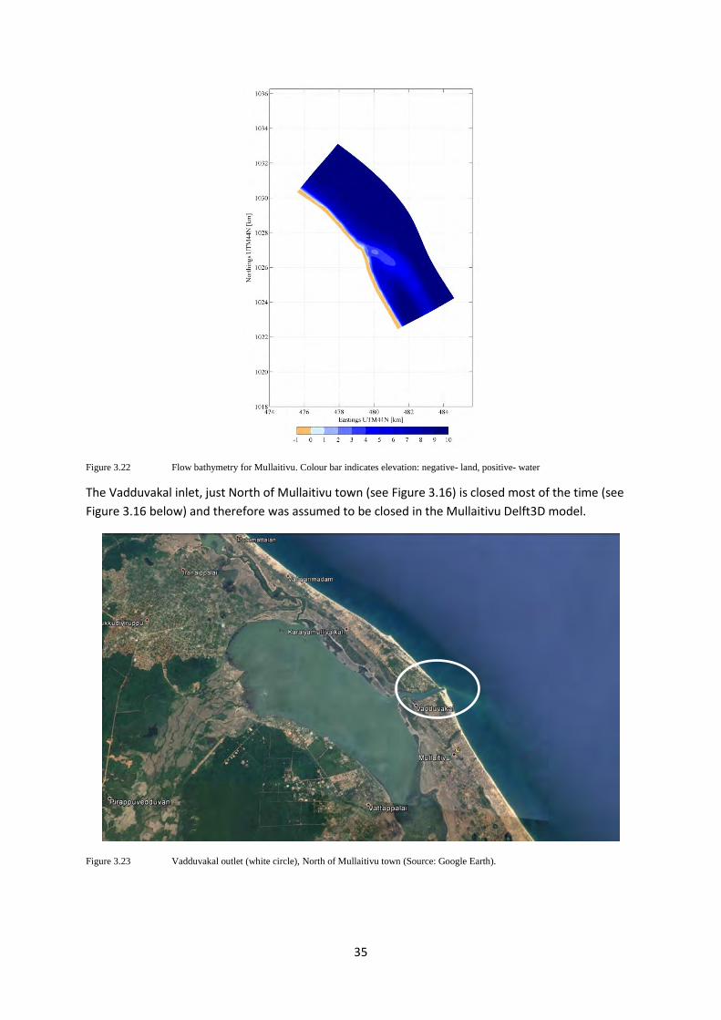
Figure 3.22 Flow bathymetry for Mullaitivu. Colour bar indicates elevation: negative- land, positive- water

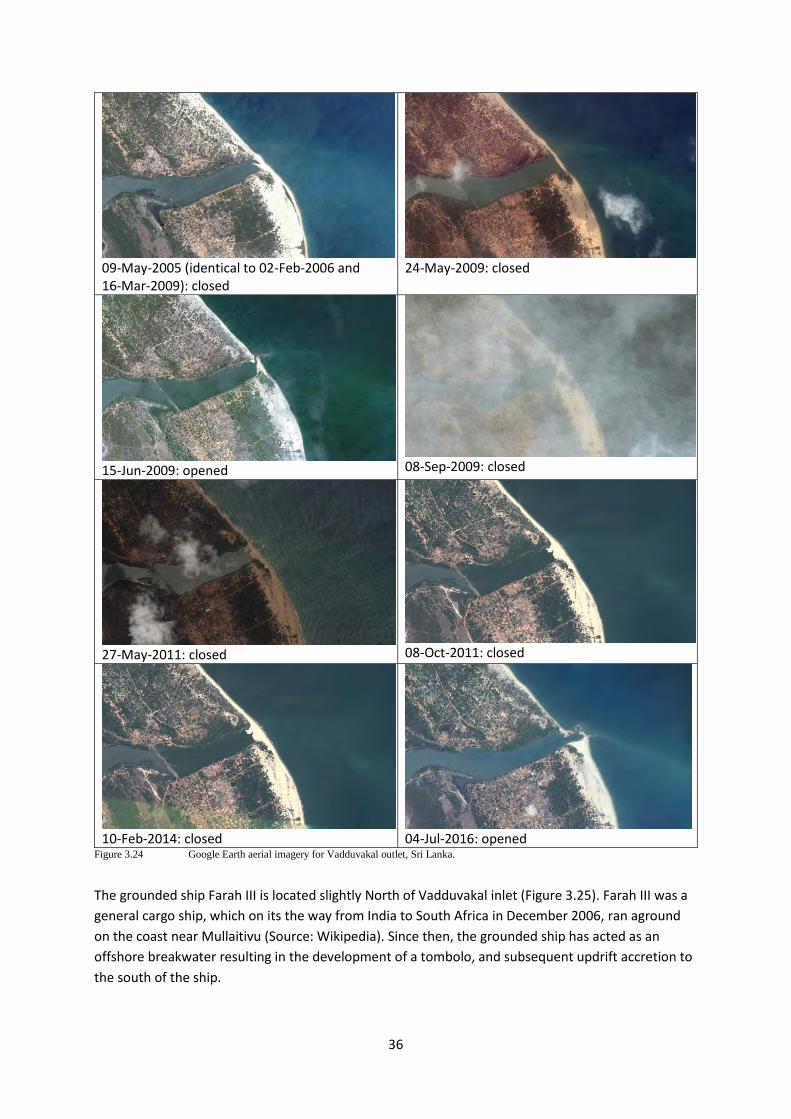
The Vadduvakal inlet, just North of Mullaitivu town (see Figure 3.16) is closed most of the time (see

Figure 3.16 below) and therefore was assumed to be closed in the Mullaitivu Delft3D model.

Figure 3.23 Vadduvakal outlet (white circle), North of Mullaitivu town (Source: Google Earth).

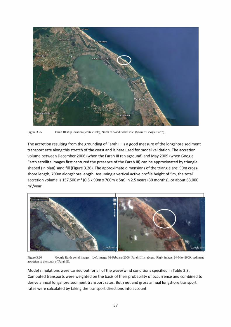
36

09-May-2005 (identical to 02-Feb-2006 and

16-Mar-2009): closed

24-May-2009: closed

15-Jun-2009: opened

08-Sep-2009: closed

27-May-2011: closed

08-Oct-2011: closed

10-Feb-2014: closed

04-Jul-2016: opened Figure 3.24 Google Earth aerial imagery for Vadduvakal outlet, Sri Lanka.

The grounded ship Farah III is located slightly North of Vadduvakal inlet (Figure 3.25). Farah III was a

general cargo ship, which on its the way from India to South Africa in December 2006, ran aground

on the coast near Mullaitivu (Source: Wikipedia). Since then, the grounded ship has acted as an

offshore breakwater resulting in the development of a tombolo, and subsequent updrift accretion to

the south of the ship.

37

Figure 3.25 Farah III ship location (white circle), North of Vadduvakal inlet (Source: Google Earth).

The accretion resulting from the grounding of Farah III is a good measure of the longshore sediment

transport rate along this stretch of the coast and is here used for model validation. The accretion

volume between December 2006 (when the Farah III ran aground) and May 2009 (when Google

Earth satellite images first captured the presence of the Farah III) can be approximated by triangle

shaped (in plan) sand fill (Figure 3.26). The approximate dimensions of the triangle are: 90m cross-

shore length, 700m alongshore length. Assuming a vertical active profile height of 5m, the total

accretion volume is 157,500 m3 (0.5 x 90m x 700m x 5m) in 2.5 years (30 months), or about 63,000

m3/year.

Figure 3.26 Google Earth aerial images: Left image: 02-Febuary-2006, Farah III is absent. Right image: 24-May-2009, sediment

accretion to the south of Farah III.

Model simulations were carried out for all of the wave/wind conditions specified in Table 3.3.

Computed transports were weighted on the basis of their probability of occurrence and combined to

derive annual longshore sediment transport rates. Both net and gross annual longshore transport

rates were calculated by taking the transport directions into account.

38

The sediment transport rates using the reduced wave climate were verified against transport rates

using the full wave climate using UNIBEST-LT and the above estimated transport rate near the

grounded Farah III ship.

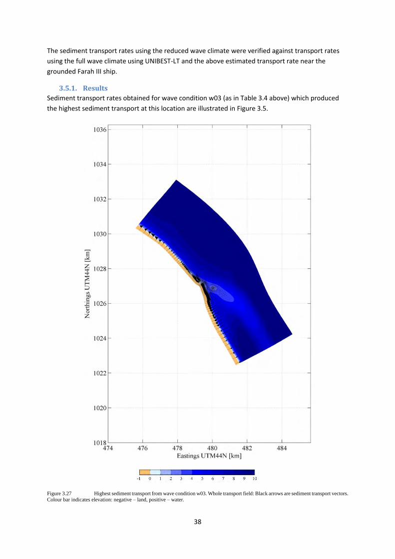
3.5.1. Results

Sediment transport rates obtained for wave condition w03 (as in Table 3.4 above) which produced

the highest sediment transport at this location are illustrated in Figure 3.5.

Figure 3.27 Highest sediment transport from wave condition w03. Whole transport field: Black arrows are sediment transport vectors.

Colour bar indicates elevation: negative – land, positive – water.

39

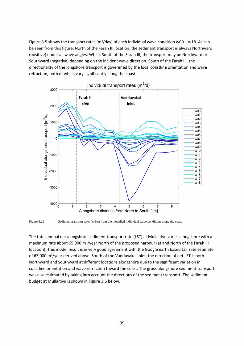
Figure 3.5 shows the transport rates (m3/day) of each individual wave condition w00 – w18. As can

be seen from this figure, North of the Farah III location, the sediment transport is always Northward

(positive) under all wave angles. While, South of the Farah III, the transport may be Northward or

Southward (negative) depending on the incident wave direction. South of the Farah III, the

directionality of the longshore transport is goverened by the local coastline orientation and wave

refraction, both of which vary significantly along the coast.

Figure 3.28 Sediment transport rates (m3/d) from the modelled individual wave conditions along the coast.

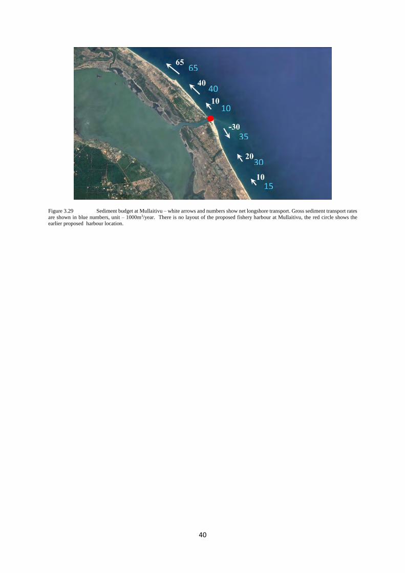
The total annual net alongshore sediment transport rate (LST) at Mullaitivu varies alongshore with a

maximum rate about 65,000 m3/year North of the proposed harbour (at and North of the Farah III

location). This model result is in very good agreement with the Google earth based LST rate estimate

of 63,000 m3/year derived above. South of the Vadduvakal inlet, the direction of net LST is both

Northward and Southward at different locations alongshore due to the significant variation in

coastline orientation and wave refraction toward the coast. The gross alongshore sediment transport

was also estimated by taking into account the directions of the sediment transport. The sediment

budget at Mullaitivu is shown in Figure 3.6 below.

Farah III

ship

Vadduvakal

Inlet

40

Figure 3.29 Sediment budget at Mullaitivu – white arrows and numbers show net longshore transport. Gross sediment transport rates

are shown in blue numbers, unit – 1000m3/year. There is no layout of the proposed fishery harbour at Mullaitivu, the red circle shows the

earlier proposed harbour location.

65

40

10

35

30

15

41

4. Conclusions and recommendations

4.1. General

4.1.1. Conclusions

• Objectives: The objective of this study is to provide reliable estimates of alongshore sediment

transport rates at the location of proposed harbours in northern Sri Lanka using state-of-the-art

coastal numerical models

• Data and models: ERA-interim global reanalysis wave data and TPXO7.2 tidal inversion data was

analysed to generate wind and wave scenarios and tidal boundary conditions for regional wave

and tidal models for northern Sri Lanka. These regional models were run to generate boundary

conditions for detailed, local Delft3D numerical models for Pesalai, Gurunagar, Point Pedro and

Mullaitivu that take tide, wind, waves and sediment transport into account.

• Alongshore sediment transport rates: based on the results of detailed, local Delft3D numerical

models, the following alongshore sediment transport rates are provided:

Table 4.1 Annual longshore sediment transport rates at the proposed harbour locations

Location Net annual alongshore sediment

transport rate (m3/year)

Gross annual alongshore

sediment transport rate (m3/year)

Pesalai 10,000 from east to west 1,000 from west to east

11,000 from east to west

Gurunagar 5,000 from west to east 5,000 from west to east

Point Pedro 30,000-150,000 from east to west 30,000-150,000 from east to west

Mullaitivu North of inlet 10,000-65,000 to

north

South of inlet 30,000(to south)-

20,000 (to north)

North of inlet 10,000-65,000 to

north

South of inlet 30,000 to north-

35,000 to south

4.1.2. Recommendations

Morphodynamic modeling: it is recommended to conduct morphodynamic modeling

studies (in which bed level changes resulting from LST gradients are fed back into wave/flow

models and vice versa within a continuous feedback loop) for the proposed harbours at

Pesalai and Point Pedro to determine the effects on the adjacent coasts, bypassing and

harbour sedimentation.

Wave measurements: it is strongly recommended to measure nearshore wave data for at

least one year using wave buoys at the locations of the proposed fishery harbours (just

outside the breaker zone). This data is currently lacking and hence wave model results

cannot be validated.

Sediment data: it is strongly recommended to measure the sediment size distribution at the

beach and in the breaker zone near the locations of the proposed fishery harbours using

sediment grabs and sieving analysis

42

4.2. Pesalai

Sediment transport: while the net annual alongshore sediment transport rate (LST) at this

location is not very large, it is not small enough to ignore. If all of the annual LST is blocked by

the eastern breakwater, eventually (over a couple of years), some erosion may occur next to

the western breakwater.

Breakwater length: most of the LST occurs below 2m water depth. Therefore, the design

cross-shore length of especially the eastern breakwater (extending to about 3.5m water

depth) might be insufficient to prevent sediment bypassing and subsequent siltation at the

harbour entrance (and even within the harbour itself) in the long term (> 2-3 years).

Morphodynamic modeling: the amount of sedimentation that might occur at the entrance

of proposed harbour (and possibly inside the harbour), and the amount of erosion that might

occur next to the western breakwater could be reliably assessed via coastal morphodynamic

modeling.

Sand Bar interaction: the Pesalai coast features a dynamic bar system that might interact

with the harbor breakwaters of the proposed fishery harbour. It is highly recommended to

study and/or model possible interaction mechanisms and effects on the adjacent coast,

bypassing and sedimentation.

Effect of high incident wave angles: along the Pesalai coast almost shore parallel, westerly

wave conditions occur that have very limited effect on longshore sediment transport rates

due to the high incident wave angles. It is recommended to study the effect of these high

incident wave angle conditions on the morphologic impact of the proposed fishery harbor.

Longshore variation: It is recommended to study the longshore sediment transport rate

along the Mannar coast using a larger model since the alongshore sediment transport rates

may vary considerably and may change direction along this coast.

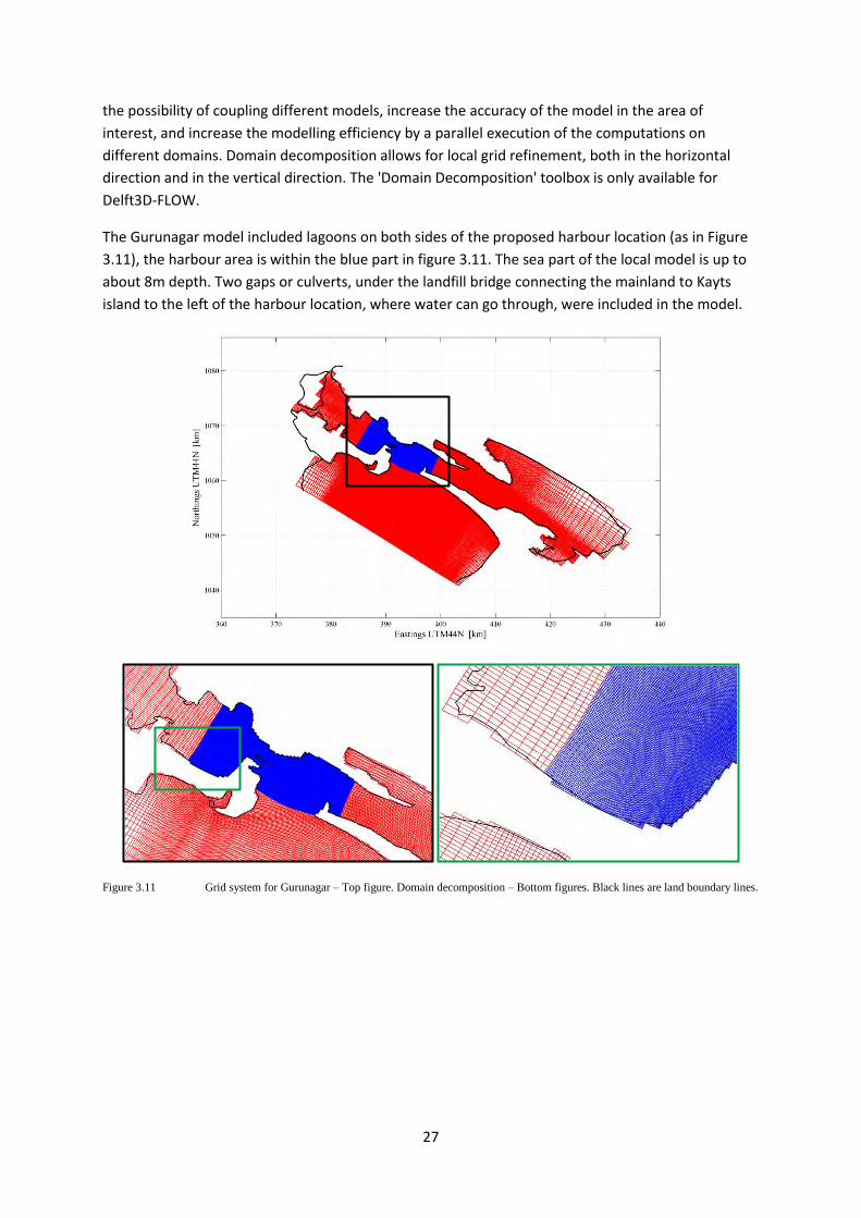
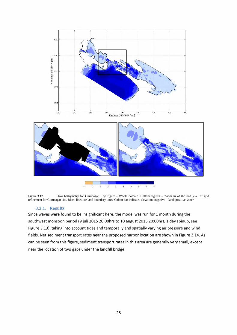
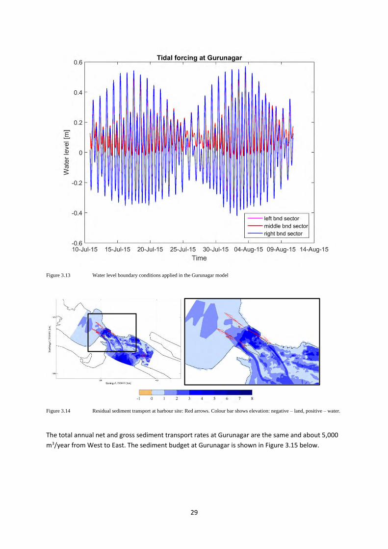
4.3. Gurunagar

Sediment transport: the sediment transport rates at this location are insignificant.

Therefore, sedimentation issues or erosion of adjacent coast at this harbour location are

unlikely.

Modeling: no further modeling is required for this location.

4.4. Point Pedro

Sediment transport: of the total net longshore sediment transport rate (LST), 30,000-

150,000 m3/year occurs seaward of the reef (from the reef down to about 3m water depth)

while 5,000-40,000 m3/year occurs between the reef and shoreline.

Reef presence: the presence of the reef in the area produces very complicated flow and

sediment transport patterns in the area which vary spatially significantly. Therefore, there is

a substantial uncertainty in the LST estimates provided, which is unavoidable.

43

Sedimentation and erosion: the calculated higher end LST (150,000 m3/year) in the area will

likely result in sedimentation/ erosion adjacent to the harbour breakwaters. This will modify

the existing flow and sediment transport patterns near the breakwaters and might result in

significant amounts of sedimentation in front of the harbour entrance and erosion next to,

especially, the western breakwater.

Morphodynamic modeling : the amount of sedimentation that might occur around (and

even inside) the proposed harbour under the high LST scenario, and the amount of erosion

that might occur next to the western breakwater could be reliably assessed via coastal

morphodynamic modeling.

4.5. Mullaitivu

Sediment transport: the net annual alongshore sediment transport rate (LST) at this location

is moderate and rather variable alongshore both in magnitude and direction. The earlier

proposed location for the harbour is right at the entrance of the inlet which was assumed to

be closed in this model. However according to local experts, the inlet opens for a few weeks

during the NE monsoon. If indeed, at some future date, it is decided to construct the harbour

right at the inlet entrance as was previously proposed, it is advisable to model the system

with the seasonally open inlet.

Morphodynamic modeling: Using the Delft3D model setup in this study, the amount of

sedimentation that might occur at the entrance of any future proposed harbour (and inside

the harbour), and the amount of erosion that might occur next to the breakwaters could be

reliably assessed via coastal morphodynamic modeling.

44

5. References

Ashton, A. D., and A. B. Murray (2006a), High-angle-wave instability and emergent shoreline shapes: 1.

Modeling of sandwaves, flying spits, and capes, J. Geophys. Res.,

Benedet, L., Dobrochinsky, J.P.F., Walstra, D.J.R. and Ranasinghe, R., 2016. A morphological study to compare

different methods of wave climate schematization and evaluate strategies to reduce erosion losses from a

nourishment project. Journal of Coastal Engineering 112:69-86, June 2016.

Booij, N., Ris, R.C. and Holthuijsen, L.H., 1999. A third-generation wave model for coastal regions. 1. Model

description and validation. Journal of Geophysical Research, 104(C4): 7649-7666.

Dhastgeib, A. and Ranasinghe, R., 2016. Delft3D model beased investigation of the possible existence of large

scale circulation patterns along the north coast of Sri Lanka. Phase 1.

Dee DP, Uppala SM, Simmons AJ, Berrisford P, Poli P, Kobayashi S, Andrae U, Balmaseda MA, Balsamo G, Bauer

P, Bechtold P, Beljaars ACM, van de Berg L, Bidlot J, Bormann N, Delsol C, Dragani R, Fuentes M, Geer AJ,

Hai erger L, Heal “B, Hers a h H, Hol EV, Isakse L, K ´ all erg P, K ˚ ohler M, Matri ardi M, M Nall AP, Monge-Sanz BM, Morcrette J-J, Park B-K, Peubey C, de Rosnay P, Tavolato C, Thepaut J-N, Vitart F. 2011. The

ERA-Interim reanal ysis: configuration and performance of the data assimilation system. Q. J. R. Meteorol. Soc.

137: 553–597. DOI:10.1002/qj.828

Duong, T.M, 2015. Climate change impacts on the stability of small tidal inlets . PhD thesis UNESCO-IHE, Delft.

Lesser, G.R., Roelvink, J.A., van Kester, J.A.T.M., Stelling, G.S., 2004. Development and validationof a three

dimensional morphological model. Journal of Coastal Engineering, 51, 883-915

Van Rijn, 2007. Unified view of sediment transport by currents and waves. I. Initiation of motion, bed

roughness and bed-load transport. Journal of Hydraulic Engineering, ASCE Vol. 133 No. 6, p649-667. (2007).

Ris, R.C., 1997. Spectral modelling of wind waves in coastal areas, PhD Thesis Delft University of Technology,

Delft.

Ris, R.C., Holthuijsen, L.H. and Booij, N., 1999. A third-generation wave model for coastal regions, Part II:

Verification. Journal of Geophysical Research, 104(C4): 7667-7682.

Sindhu B, Suresh I, Unnikrishnan A S, Bhatkar N V, Neetu S, Michael G S, 2007. Improved bathymetric datasets

for the shallow water regions in the Indian Ocean. J. Earth Syst. Sci.: 116(3); 2007; 261-274.

Swan, B., 1983. An introduction to the coastal geomorphology of Sri Lanka. National museum of Sri Lanka

WL | Delft Hydraulics, 1999. Modification first-guess SWAN & benchmark tests for SWAN. Report H3515.

WL | Delft Hydraulics, 2000. SWAN: Physical formulations and data for validation. Report H3528

Zubair, L. and Chandimala, J, 2006. Epochal Changes in ENSO – Lanka. Journal of hydrometeorology, Vol. 7, No.

6, p. 1237-1246.

45

A. Wave modeling

A.1 Objectives and approach

The main objective of the wave modeling is to provide nearshore wave climates for the Delft3D

numerical models of the potential harbour locations. In order to simulate wave conditions along the

four study sites, a large-scale wave model is set up for North Sri Lanka. This model is then applied to

simulate scenarios based on the ERA-interim global reanalysis. Model results have been used to

produce wave input files for UNIBEST-LT and to reconstruct near wave time series by means of wave

transformation matrices. Finally, these nearshore wave time series have been reduced into a limited

number of representative wave conditions using the energy flux method (Benedet et al, 2016)). This

is done for practical reasons and to reduce computational time of the numerical models that

otherwise would have to be run all of the scenarios modelled using SWAN.

The wave model applied is the third-generation fully spectral SWAN model developed by Delft

University of Technology. Deltares has integrated the SWAN model with its Delft3D modeling suite.

“e tio s A.3 to A.6 des ri e the a aila le a e data, odel set up, odel s e ario s a d odel

results. First a brief description of SWAN is given

A.2 SWAN wave model

SWAN is a third-generation shallow water wave model, which is based on the discrete spectral action

balance equation. The model is fully spectral and solves for the total range of wave frequencies and

wave directions, which implies that short-crested random wave fields propagating simultaneously

from widely different directions can be accommodated. The wave propagation is based on linear

wave theory, including the effect of currents. The processes of wind generation, dissipation and non-

linear wave-wave interactions are represented explicitly with state-of-the-art third-generation

formulations. The model includes all relevant physical processes of wave propagation, generation

and dissipation, such as:

• Refraction due to variations in depth and currents.

• Shoaling.

• Wave growth due to wind.

• Wave dissipation due to white-capping.

• Dissipation due to surf-breaking.

• Dissipation due to bottom friction.

• Wave-blocking due to an opposing current.

• Non-linear wave-wave interaction in deep water (quadruplets).

• Non-linear wave-wave interaction in shallow water (triads).

• Transmission and reflection of wave energy at obstacles.

Diffraction is not modelled explicitly by SWAN, but the effects of directional spreading and growth of

waves due to wind dominate diffraction effects in many cases. A more complete description of the

SWAN wave model can be found in Booij et al. (1999).

The SWAN wave model has been successfully validated and verified in several laboratory and

complex field cases (e.g. Ris, 1997; Ris et al., 1999). A large number of these cases and additional

academic tests have been combined to prepare a testbank for this model. This testbank is a software

environment containing a series of test cases for the SWAN model. It was developed by Deltares

(formerly Delft Hydraulics) on request of the Dutch National Institute for Coastal and Marine

Management (WL | Delft Hydraulics, 1999; WL | Delft Hydraulics, 2000). This testbank includes

academic situations (e.g. shoaling and refraction tests), laboratory situations and field measurements

46

that are used to test new versions of the model in comparison with other versions. The version of

SWAN used in this study is 40.72A.

A.3 Wave data: ERA-interim

ECMWF (European Centre for Medium-Range Weather Forecasts) wind and wave data were used in

this study. In particular, the most recent reanalysis of this data was used (Dee et al., 2011). The data

are 6 hourly, starting from 1979 and are available on a global grid with a resolution of about 0.75° x

0.75°. The data contains information on wind speed (U10), wind direction as well as on wave

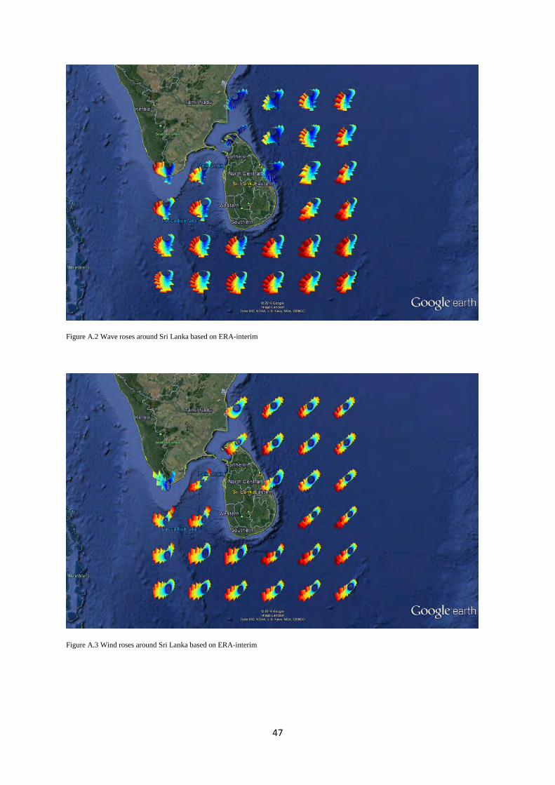
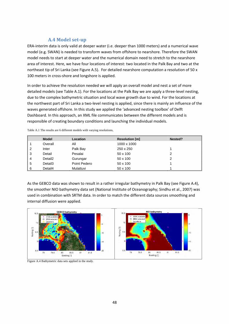
conditions (wave height, period and direction). Figure A.2 shows offshore wave roses around Sri

Lanka. Figure A.3 shows offshore windroses around Sri Lanka.

In Sri Lanka there are two monsoons dominating the waves and winds. The south-western monsoon

runs between May and September and results in higher waves and wind from the southwest. The

north-eastern monsoon runs between October and January and results in higher waves and wind

from the northeast. In the period in between wind and waves shift from one dominant direction to

the other.

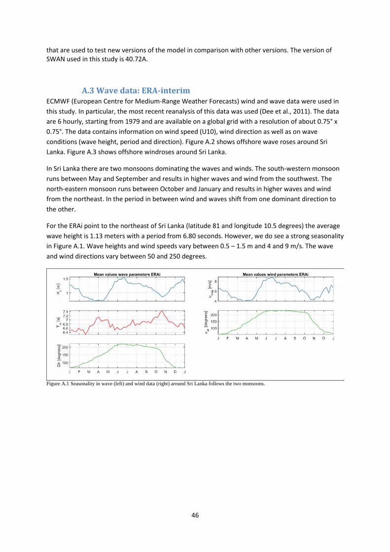
For the ERAi point to the northeast of Sri Lanka (latitude 81 and longitude 10.5 degrees) the average

wave height is 1.13 meters with a period from 6.80 seconds. However, we do see a strong seasonality

in Figure A.1. Wave heights and wind speeds vary between 0.5 – 1.5 m and 4 and 9 m/s. The wave

and wind directions vary between 50 and 250 degrees.

Figure A.1 Seasonality in wave (left) and wind data (right) around Sri Lanka follows the two monsoons.

47

Figure A.2 Wave roses around Sri Lanka based on ERA-interim

Figure A.3 Wind roses around Sri Lanka based on ERA-interim

48

A.4 Model set-up

ERA-interim data is only valid at deeper water (i.e. deeper than 1000 meters) and a numerical wave

model (e.g. SWAN) is needed to transform waves from offshore to nearshore. Therefore the SWAN

model needs to start at deeper water and the numerical domain need to stretch to the nearshore

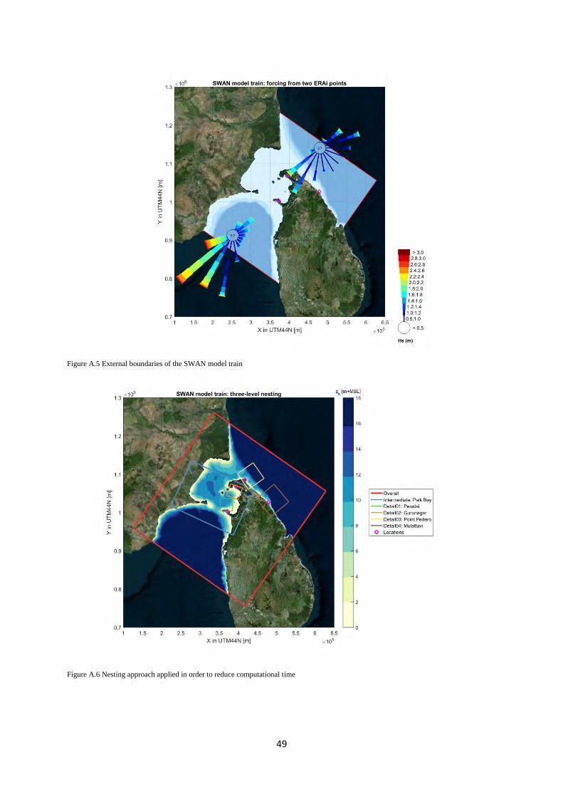
area of interest. Here, we have four locations of interest: two located in the Palk Bay and two at the

northeast tip of Sri Lanka (see Figure A.5). For detailed nearshore computation a resolution of 50 x

100 meters in cross-shore and longshore is applied.

In order to achieve the resolution needed we will apply an overall model and nest a set of more

detailed models (see Table A.1). For the locations at the Palk Bay we are apply a three-level nesting,

due to the complex bathymetric situation and local wave growth due to wind. For the locations at

the northwest part of Sri Lanka a two-level nesting is applied, since there is mainly an influence of the

waves generated offshore. In this study we applied the ad a ed esti g tool o of Delft Dashboard. In this approach, an XML file communicates between the different models and is

responsible of creating boundary conditions and launching the individual models.

Table A.1 The results are 6 different models with varying resolutions,

Model Location Resolution [m] Nested?

1 Overall All 1000 x 1000

2 Inter Palk Bay 250 x 250 1

3 Detail Pesalai 50 x 100 2

4 Detail2 Gurungar 50 x 100 2

5 Detail3 Point Pedero 50 x 100 1

6 Detail4 Mulattuvi 50 x 100 1

As the GEBCO data was shown to result in a rather irregular bathymetry in Palk Bay (see Figure A.4),

the smoother NIO bathymetry data set (National Institute of Oceanography; Sindhu et al., 2007) was

used in combination with SRTM data. In order to match the different data sources smoothing and

internal diffusion were applied.

Figure A.4 Bathymetric data sets applied in the study.

49

Figure A.5 External boundaries of the SWAN model train

Figure A.6 Nesting approach applied in order to reduce computational time

50

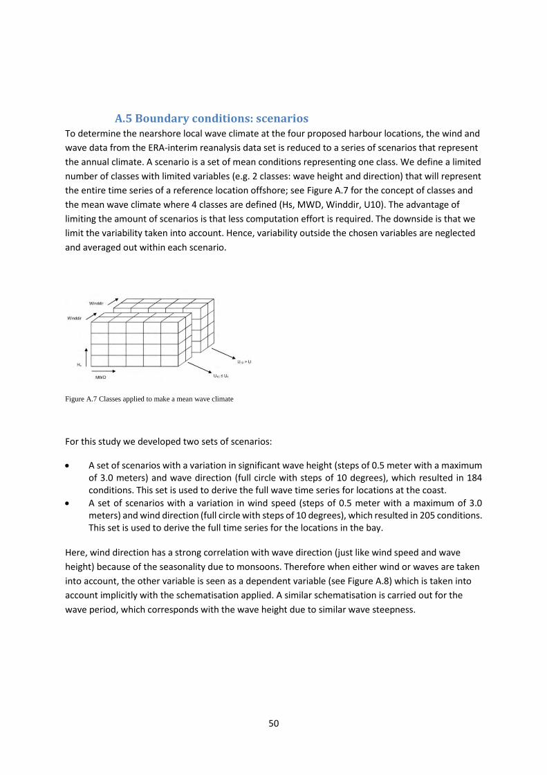
A.5 Boundary conditions: scenarios

To determine the nearshore local wave climate at the four proposed harbour locations, the wind and

wave data from the ERA-interim reanalysis data set is reduced to a series of scenarios that represent

the annual climate. A scenario is a set of mean conditions representing one class. We define a limited

number of classes with limited variables (e.g. 2 classes: wave height and direction) that will represent

the entire time series of a reference location offshore; see Figure A.7 for the concept of classes and

the mean wave climate where 4 classes are defined (Hs, MWD, Winddir, U10). The advantage of

limiting the amount of scenarios is that less computation effort is required. The downside is that we

limit the variability taken into account. Hence, variability outside the chosen variables are neglected

and averaged out within each scenario.

Figure A.7 Classes applied to make a mean wave climate

For this study we developed two sets of scenarios:

A set of scenarios with a variation in significant wave height (steps of 0.5 meter with a maximum

of 3.0 meters) and wave direction (full circle with steps of 10 degrees), which resulted in 184

conditions. This set is used to derive the full wave time series for locations at the coast.

A set of scenarios with a variation in wind speed (steps of 0.5 meter with a maximum of 3.0

meters) and wind direction (full circle with steps of 10 degrees), which resulted in 205 conditions.

This set is used to derive the full time series for the locations in the bay.

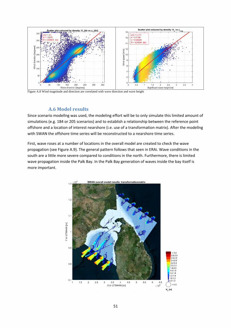
Here, wind direction has a strong correlation with wave direction (just like wind speed and wave

height) because of the seasonality due to monsoons. Therefore when either wind or waves are taken

into account, the other variable is seen as a dependent variable (see Figure A.8) which is taken into

account implicitly with the schematisation applied. A similar schematisation is carried out for the

wave period, which corresponds with the wave height due to similar wave steepness.

51

Figure A.8 Wind magnitude and direction are correlated with wave direction and wave height

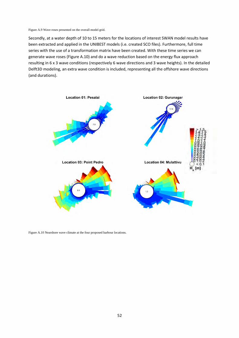
A.6 Model results

Since scenario modellng was used, the modeling effort will be to only simulate this limited amount of

simulations (e.g. 184 or 205 scenarios) and to establish a relationship between the reference point

offshore and a location of interest nearshore (i.e. use of a transformation matrix). After the modellng

with SWAN the offshore time series will be reconstructed to a nearshore time series.

First, wave roses at a number of locations in the overall model are created to check the wave

propagation (see Figure A.9). The general pattern follows that seen in ERAi. Wave conditions in the

south are a little more severe compared to conditions in the north. Furthermore, there is limited

wave propagation inside the Palk Bay. In the Palk Bay generation of waves inside the bay itself is

more important.

52

Figure A.9 Wave roses presented on the overall model grid.

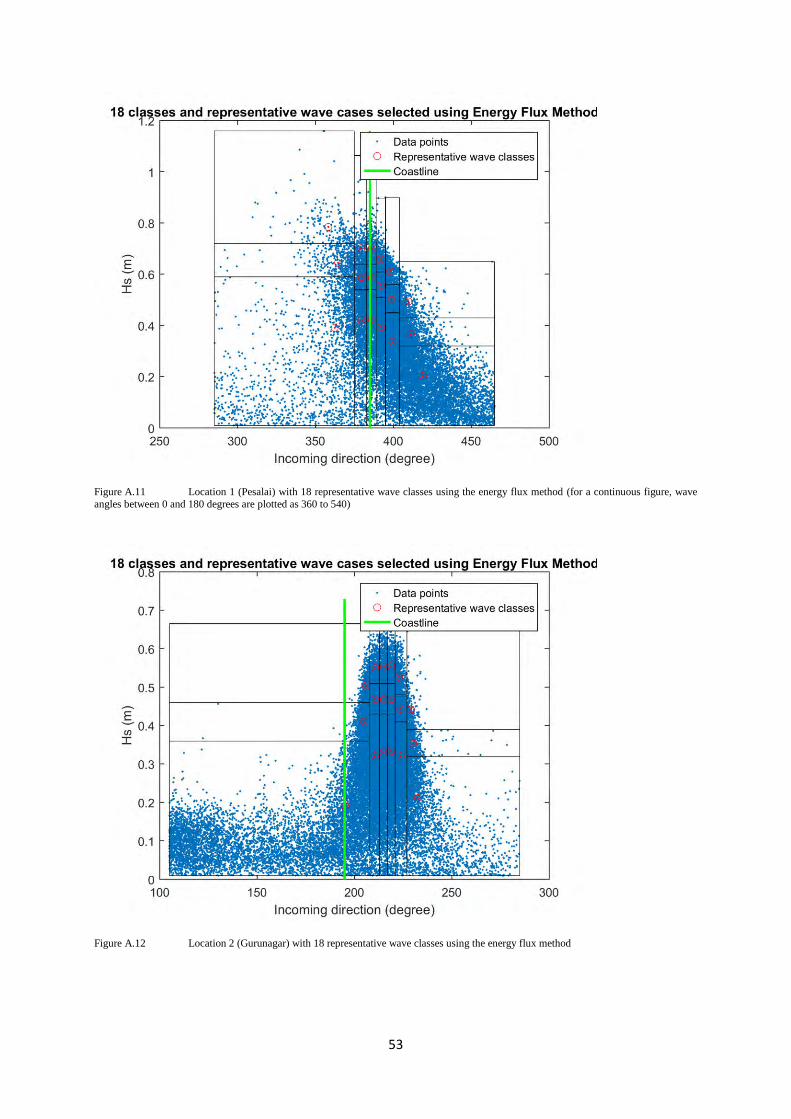
Secondly, at a water depth of 10 to 15 meters for the locations of interest SWAN model results have

been extracted and applied in the UNIBEST models (i.e. created SCO files). Furthermore, full time

series with the use of a transformation matrix have been created. With these time series we can

generate wave roses (Figure A.10) and do a wave reduction based on the energy flux approach

resulting in 6 x 3 wave conditions (respectively 6 wave directions and 3 wave heights). In the detailed

Delft3D modeling, an extra wave condition is included, representing all the offshore wave directions

(and durations).

Figure A.10 Nearshore wave climate at the four proposed harbour locations.

53

Figure A.11 Location 1 (Pesalai) with 18 representative wave classes using the energy flux method (for a continuous figure, wave

angles between 0 and 180 degrees are plotted as 360 to 540)

Figure A.12 Location 2 (Gurunagar) with 18 representative wave classes using the energy flux method

54

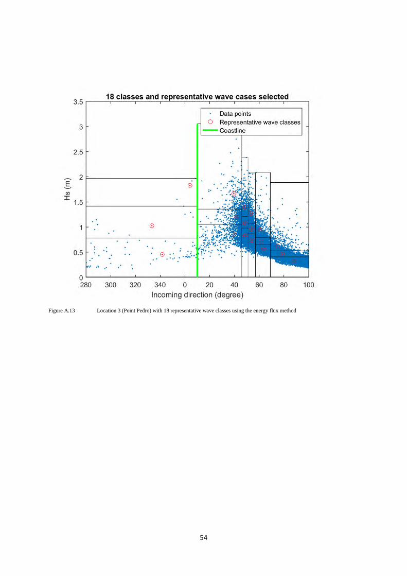
Figure A.13 Location 3 (Point Pedro) with 18 representative wave classes using the energy flux method

55

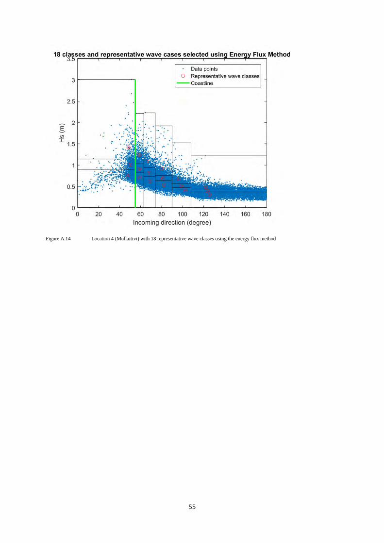
Figure A.14 Location 4 (Mullaitivi) with 18 representative wave classes using the energy flux method

56

B. Tidal modeling

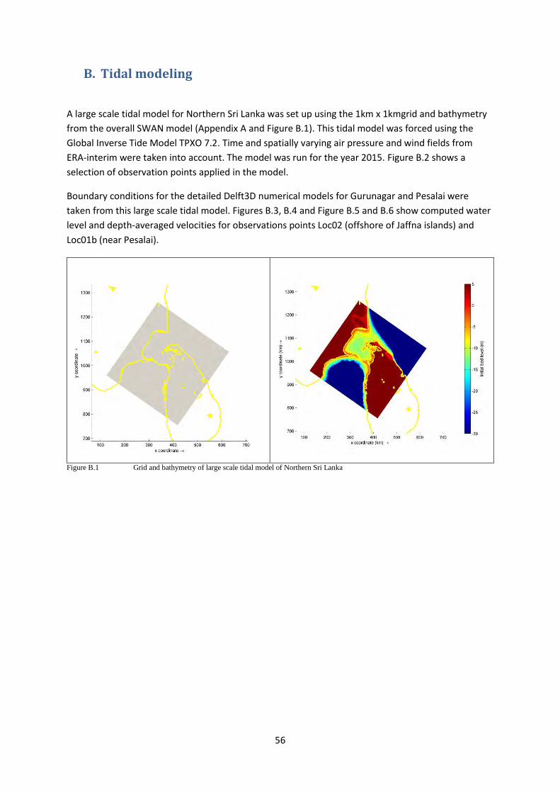
A large scale tidal model for Northern Sri Lanka was set up using the 1km x 1kmgrid and bathymetry

from the overall SWAN model (Appendix A and Figure B.1). This tidal model was forced using the

Global Inverse Tide Model TPXO 7.2. Time and spatially varying air pressure and wind fields from

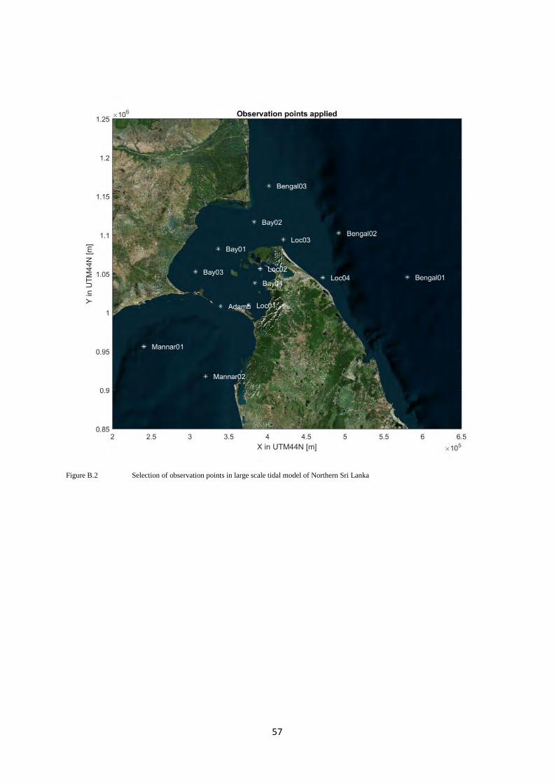
ERA-interim were taken into account. The model was run for the year 2015. Figure B.2 shows a

selection of observation points applied in the model.

Boundary conditions for the detailed Delft3D numerical models for Gurunagar and Pesalai were

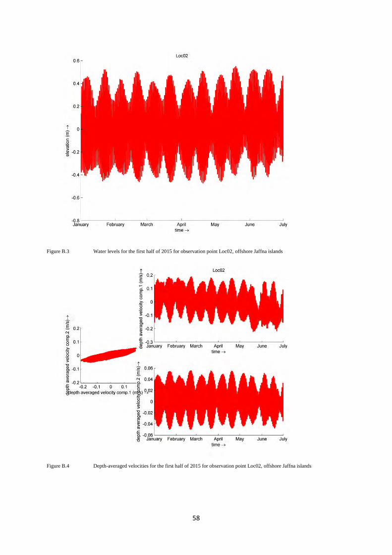
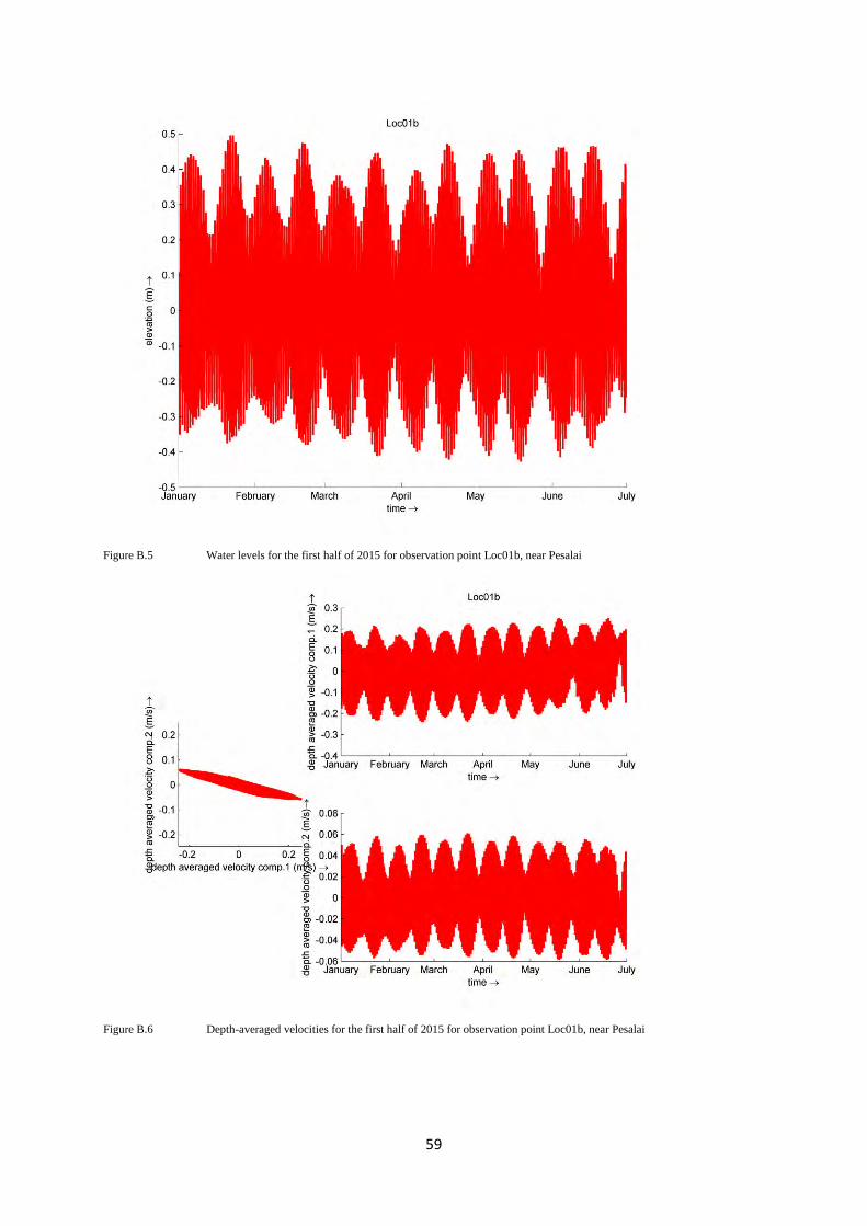
taken from this large scale tidal model. Figures B.3, B.4 and Figure B.5 and B.6 show computed water

level and depth-averaged velocities for observations points Loc02 (offshore of Jaffna islands) and

Loc01b (near Pesalai).

Figure B.1 Grid and bathymetry of large scale tidal model of Northern Sri Lanka

57

Figure B.2 Selection of observation points in large scale tidal model of Northern Sri Lanka

58

Figure B.3 Water levels for the first half of 2015 for observation point Loc02, offshore Jaffna islands

Figure B.4 Depth-averaged velocities for the first half of 2015 for observation point Loc02, offshore Jaffna islands

59

Figure B.5 Water levels for the first half of 2015 for observation point Loc01b, near Pesalai

Figure B.6 Depth-averaged velocities for the first half of 2015 for observation point Loc01b, near Pesalai

60

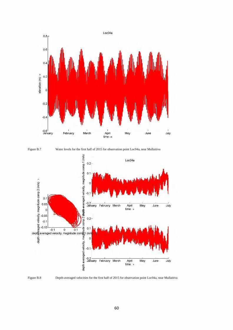
Figure B.7 Water levels for the first half of 2015 for observation point Loc04a, near Mullaitivu

Figure B.8 Depth-averaged velocities for the first half of 2015 for observation point Loc04a, near Mullaitivu