Delineation of gravel-bed clusters via factorial kriging 2 ... 1 Delineation of gravel-bed clusters...

1

Delineation of gravel-bed clusters via factorial kriging 1

Fu-Chun Wu (corresponding author: [email protected]) 2

Department of Bioenvironmental Systems Engineering, National Taiwan University, Taipei, Taiwan. 3

Chi-Kuei Wang 4

Department of Geomatics, National Cheng Kung University, Tainan, Taiwan. 5

Guo-Hao Huang 6

Geographic Information System Research Center, Feng Chia University, Taichung, Taiwan. 7

Abstract 8

Gravel-bed clusters are the most prevalent microforms that affect local flows and sediment transport. 9

A growing consensus is that the practice of cluster delineation should be based primarily on bed 10

topography rather than grain sizes. Here we present a novel approach for cluster delineation using 11

patch-scale high-resolution digital elevation models (DEMs). We use a geostatistical interpolation 12

method, i.e., factorial kriging, to decompose the short- and long-range (grain- and microform-scale) 13

DEMs. The required parameters are determined directly from the scales of the nested variograms. 14

The short-range DEM exhibits a flat bed topography, yet individual grains are sharply outlined, 15

making the short-range DEM a useful aid for grain segmentation. The long-range DEM exhibits a 16

smoother topography than the original full DEM, yet groupings of particles emerge as small-scale 17

bedforms, making the contour percentile levels of the long-range DEM a useful tool for cluster 18

identification. Individual clusters are delineated using the segmented grains and identified clusters 19

via a range of contour percentile levels. Our results reveal that the density and total area of delineated 20

clusters decrease with increasing contour percentile level, while the mean grain size of clusters and 21

average size of anchor clast (i.e., the largest particle in a cluster) increase with the contour percentile 22

level. These results support the interpretation that larger particles group as clusters and protrude 23

higher above the bed than other smaller grains. A striking feature of the delineated clusters is that 24

anchor clasts are invariably greater than the D90 of the grain sizes even though a threshold anchor 25

size was not adopted herein. The average areal fractal dimensions (Hausdorff-Besicovich dimensions 26

of the projected areas) of individual clusters, however, demonstrate that clusters delineated with 27

different contour percentile levels exhibit similar planform morphologies. Comparisons with a 28

compilation of existing field data show consistency with the cluster properties documented in a wide 29

variety of settings. This study thus points toward a promising, alternative DEM-based approach to 30

characterizing sediment structures in gravel-bed rivers. 31

Keywords: Gravel-bed rivers, clusters, delineation, factorial kriging, digital elevation model (DEM). 32

2

1. Introduction 33

Gravel-bed rivers exhibit a wide variety of bedforms ranging in scale from microforms (e.g., 34

imbrication, cluster), mesoforms (e.g., transverse rib, stone cell, step-pool, pool-riffle), macroforms 35

(e.g., bar), to megaforms (e.g., floodplain, terraces) (Hassan et al., 2008). Among these, clusters are 36

the most prevalent microforms, observed to cover 10-50% of the bed surface (Wittenberg, 2002; 37

Papanicolaou et al., 2012). Clusters have drawn much attention from river scientists and engineers 38

due to their impacts on: (1) local turbulence structures (Buffin-Bélanger and Roy, 1998; Lawless and 39

Robert, 2001a; Lacey and Roy, 2007; Strom et al., 2007; Hardy et al., 2009; Curran and Tan, 2014a; 40

Rice et al., 2014), (2) flow resistance (Hassan and Reid, 1990; Clifford et al., 1992; Lawless and 41

Robert, 2001b; Smart et al., 2002), (3) sediment transport (Brayshaw et al., 1983; Brayshaw, 1984, 42

1985; Billi, 1988; Paola and Seal, 1995; Hassan and Church, 2000; Strom et al., 2004), and (4) bed 43

stability (Reid et al., 1992; Wittenberg and Newson, 2005; Oldmeadow and Church, 2006; Mao, 44

2012). Besides, clusters also provide insights into the flow and sediment supply conditions of their 45

formation (Papanicolaou et al., 2003; Wittenberg and Newson, 2005; Strom and Papanicolaou, 2009; 46

Mao et al., 2011). 47

The term ‘clusters’ was traditionally used by many researchers to refer to the so-called ‘pebble 48

clusters’, which normally comprise three components: obstacle, stoss, and wake (Brayshaw, 1984). 49

The obstacle is a large clast providing an anchor for cluster formation; upstream of the obstacle is an 50

accumulation of smaller particles that constitute the stoss zone; downstream of the obstacle is a wake 51

zone characterized by deposition of fine material. More recently, clusters have been perceived more 52

broadly to refer to “discrete, organized groupings of larger particles that protrude above the local 53

mean bed level” (Strom and Papanicolaou, 2008; Curran and Tan, 2014a). Using this broad working 54

definition, researchers have identified cluster microforms with a variety of shapes, such as rhombic 55

clusters, complex clusters, line clusters, comet clusters, ring clusters, heap clusters, triangle clusters, 56

and diamond clusters (e.g., de Jong and Ergenzinger, 1995; Wittenberg, 2002; Strom and 57

Papanicolaou, 2008; Hendrick et al., 2010). Papanicolaou et al. (2012) used the areal fractal 58

(Hausdorff-Besicovich) dimensions of the projected areas to discriminate the planform morphologies 59

3

of the clusters. 60

Although the broad definition of clusters has opened up new avenues for recent progress in 61

cluster research, to date identification of clusters still relies largely on visual inspection (e.g., 62

Entwistle et al., 2008; Strom and Papanicolaou, 2008; Hendrick et al., 2010; L’Amoreaux and 63

Gibson, 2013). A set of predetermined criteria for cluster identification are normally adopted in these 64

studies. A typical example is given here: (1) A cluster consists of a minimum number of (e.g., 3 or 4) 65

abutting or imbricated particles; (2) at least one of these particles is an anchor clast greater than the 66

specified grain size (e.g., D50 or D84) of the bed surface; (3) a cluster protrudes above the surrounding 67

bed surface (e.g., Oldmeadow and Church, 2006; Hendrick et al., 2010). As can be seen, specifying a 68

minimum number of constituent particles and a threshold grain size for anchor clast is somewhat 69

arbitrary and based on the rule of thumb. The subjectivity of the ‘gestalt sampling’ could produce 70

operational bias. In particular, researchers have found it extremely difficult to visually recognize bed 71

structures whose dimensions are of the same order of magnitude as their spacing and the grain sizes 72

of their constituent particles (Entwistle et al., 2008; L’Amoreaux and Gibson, 2013). 73

In laboratory settings, identification of clusters was recently advanced by a combined analysis 74

of bed-surface images and digital elevation models (DEMs) (Curran and Tan, 2014a; Curran and 75

Waters, 2014), with the procedure described as follows. First, clusters are visually identified by the 76

particle arrangements shown in the digital photos. Then, the visually identified clusters are verified 77

with the DEM, checking whether clusters are discrete and protruding above the mean bed level by a 78

specified minimum height (e.g., D85 or D95). Last, each verified cluster is confirmed by checking 79

whether the cluster consists of a recognizable anchor clast > D90, around which at least two particles 80

> D50 were deposited. In contrast to the previous laboratory approaches that used only images or 81

DEMs to identify clusters (Mao, 2012; Piedra et al., 2012; Heays et al., 2014), the combined use of 82

images and DEMs represents technological progress, providing a more robust approach. This 83

approach, however, continues to rely on visual inspection at the identification stage and specification 84

of some quantitative criteria (e.g., threshold protrusion height and grain sizes) at the verification and 85

confirmation stages, thus is prone to a certain degree of subjective judgment. 86

4

Attempts to apply advanced methods to studies of field clusters have been made by two groups 87

of researchers. The first group (Entwistle et al., 2008) used the DEM derived from terrestrial laser 88

scanning (TLS) and an optimized moving window to compute the local standard deviations (SD) of 89

bed elevation across a study reach. The resultant SD surface was interrogated to extract the SD that 90

corresponded to the observed clusters. The statistics derived from the classified SD were then applied 91

to a validation DEM to produce a map of predicted clusters. The density and spacing metrics of these 92

predicted clusters were consistent with field observations, while the shapes and constituent grains of 93

individual clusters were not resolvable with this statistical approach. By contrast, the second group 94

(L’Amoreaux and Gibson, 2013) used image analysis and nearest neighbor statistics to quantify the 95

relative abundance and spatial scale of clusters, yet individual clusters were not resolvable with such 96

spatial statistics. The most debatable aspect of this approach is, perhaps, to collectively treat large 97

grains (> D84) and medium grains (between D50 and D84) as clusters just because they were found in 98

proximity to similar grains more frequently than the spatially random null hypothesis would predict. 99

The lack of a topographic component in this type of analysis, however, made clusters a 2D statistical 100

feature of plane sampling rather than a 3D morphological feature of bed structures. 101

While the use of DEMs in cluster identification has proved promising in laboratory settings, 102

extending this approach to field studies would require: (1) high-resolution DEMs that resolve both 103

the grain- and microform-scale topographies, and (2) DEM-based delineation of clusters. 104

High-resolution DEMs that capture grain-scale details over the reach-scale extent are now achievable 105

using the hyperscale survey methods, such as TLS or Structure-from-Motion photogrammetry (see 106

reviews by Milan and Heritage (2012) and Brasington et al. (2012)). However, a standardized 107

DEM-based method for delineating clusters is still lacking. Here we present a novel, DEM-based 108

approach for cluster delineation. This approach is facilitated by the feature recognition capability of 109

the factorial kriging that decomposes the grain- and microform-scale components of DEM. The 110

grain-scale DEM serves as an aid for segmentation of grain boundaries, while the microform-scale 111

DEM is used to identify individual clusters. The delineated clusters are compared with a compilation 112

of existing field data to confirm the robustness of the presented approach. 113

5

2. Factorial kriging 114

The DEM of a gravel-bed surface may be considered as a random field of spatial elevation data 115

(e.g., Matheron, 1971; Journel and Huijbregts, 1978; Furbish, 1987; Robert, 1988; Goovaerts, 1997; 116

Nikora et al., 1998), where the dependency between the bed elevations at two locations is expressed 117

as a function of the spatial lag, i.e., the separation distance and direction between the two locations. 118

The organization of the gravel-bed surface has been investigated by many researchers using the 119

semivariogram (or simply called variogram) (e.g., Robert, 1988, 1991; Nikora et al., 1998; Butler et 120

al., 2001; Marion et al., 2003; Aberle and Nikora, 2006; Cooper and Tait, 2009; Hodge et al., 2009; 121

Mao et al., 2011; Huang and Wang, 2012; Curran and Waters, 2014), which is a second-order 122

structure function summarizing all the information about the spatial variation in bed elevation over a 123

range of scales. The empirical (also termed sample or experimental) 2D variogram of the DEM, 124

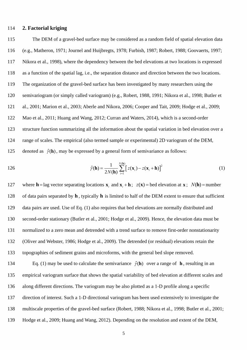
denoted as ˆ( ) h , may be expressed by a general form of semivariance as follows: 125

( )

2

1

1ˆ( ) ( ) ( )

2 ( )

N

i ii

z zN

h

h x x hh

(1) 126

where h lag vector separating locations and i i x x h ; ( )z x bed elevation at x ; ( )N h number 127

of data pairs separated by h , typically h is limited to half of the DEM extent to ensure that sufficient 128

data pairs are used. Use of Eq. (1) also requires that bed elevations are normally distributed and 129

second-order stationary (Butler et al., 2001; Hodge et al., 2009). Hence, the elevation data must be 130

normalized to a zero mean and detrended with a trend surface to remove first-order nonstationarity 131

(Oliver and Webster, 1986; Hodge et al., 2009). The detrended (or residual) elevations retain the 132

topographies of sediment grains and microforms, with the general bed slope removed. 133

Eq. (1) may be used to calculate the semivariance ˆ( ) h over a range of h , resulting in an 134

empirical variogram surface that shows the spatial variability of bed elevation at different scales and 135

along different directions. The variogram may be also plotted as a 1-D profile along a specific 136

direction of interest. Such a 1-D directional variogram has been used extensively to investigate the 137

multiscale properties of the gravel-bed surface (Robert, 1988; Nikora et al., 1998; Butler et al., 2001; 138

Hodge et al., 2009; Huang and Wang, 2012). Depending on the resolution and extent of the DEM, 139

6

and whether bedforms are present, the variogram profile may exhibit single or multiple scaling 140

regions that correspond to different scales of the bed structures. Figure 1 demonstrates a schematic 141

empirical variogram profile (solid circles) that exhibits two scaling regions. The first region, with the 142

lags ranging between 1[0, ],a corresponds to the grain-scale structure. The second region, with the 143

lags ranging between 1 2[ , ],a a corresponds to the microform-scale structure. At lags greater than 2a , 144

the semivariance remains a constant sill value, which corresponds to a saturation region where the 145

spatial dependency is minimal and no longer varies with the lag. The variogram profile may exhibit 146

more than two scaling regions if bedforms at larger scales (e.g., mesoform or macroform) are also 147

present. On the contrary, the variogram profile may not reach a constant sill if the extent of the DEM 148

is not large enough or bed elevations are not completely stationary (Hodge et al., 2009; Huang and 149

Wang, 2012). It should be noted here that to capture the mean scales of sediment grains and 150

microforms in all directions, an omni-directional variogram profile integrating all directional 151

variograms was used in this study, following the suggestion of Isaaks and Srivastava (1989). 152

To be useful in the kriging, the empirical variogram profile is fitted with a continuous, basic 153

mathematical model. For a variogram profile that exhibits multiple scales, a nested model (i.e., a 154

linear combination of basic mathematical models) may be used to describe the multiscale bed 155

structure. For example, linear, exponential, and spherical models are among the most frequently used 156

basic mathematical models (Atkinson, 2004; Webster and Oliver, 2007). For the schematic diagram 157

shown in Fig. 1, the empirical variogram is fitted with a double spherical model (red line), which is a 158

nested model that combines linearly two spherical models (blue lines), one with a short range 1a and 159

the other with a long range 2a , which may be expressed as follows (Webster and Oliver, 2007): 160

7

1 2

1

2

3 3

1 2 11 1 2 2

( ) ( )

3

1 21 2 1

2 2( )

( )

3 1 3 1 for 0

2 2 2 2

3 1( ) ( ) ( ) for

2 2

h h

h

h

h h h hc c h a

a a a a

h hh h h c c a h

a a

21

2

1 2 2

( )( )

for hh

a

c c h a

(2) 161

where ( )h theoretical variogram model, to be differentiated from the empirical variogram ˆ( )h 162

given in Eq. (1), here h h is omni-directional lag; 1 2( ) and ( )h h are short- and long- range 163

variograms; 1 1( , )a c and 2 2( , )a c are, respectively, the pairs of (range, sill) of 1 2( ) and ( )h h , 164

evaluated using, e.g., the gstat package of the open source software R (Pebesma, 2004). In this study, 165

the range values 1 2 and a a correspond to the grain and microform scales, respectively. Once ( )h is 166

decomposed into 1 2( ) and ( )h h , they can be used in the factorial kriging, described as follows. 167

Factorial kriging (FK) is a geostatistical interpolation method devised by Matheron (1982) that 168

allows the decomposed components of a regionalized variable to be individually estimated and 169

mapped. FK has been widely applied in a variety of research fields, e.g., image processing and 170

analysis for remote sensing (Wen and Sinding-Larsen, 1997; Oliver et al., 2000; Van Meirvenne 171

and Goovaerts, 2002; Goovaerts et al., 2005a; Ma et al., 2014), water and soil environmental 172

monitoring (Goovaerts et al., 1993; Goovaerts and Webster, 1994; Dobermann et al., 1997; Bocchi et 173

al., 2000; Castrignanò et al., 2000; Alary and Demougeot-Renard, 2010; Allaire et al., 2012; Lv et al., 174

2013; Bourennane et al., 2017), geophysics and geochemistry exploration (Galli et al., 1984; 175

Sandjivy, 1984; Jaquet, 1989; Yao et al., 1999; Dubrule, 2003; Reis et al., 2004), risk assessment and 176

crime management (Goovaerts et al., 2005b; Kerry et al., 2010), among many others. Despite its 177

extensive application, to date FK has not been applied to the delineation of cluster microforms. 178

The theory of FK can be found in textbooks dedicated to geostatistics (e.g., Goovaerts, 1997; 179

Webster and Oliver, 2007), thus it is only briefly summarized here. Kriging generally refers to 180

8

geostatistical predictions that estimate the value at any point using a set of nearby sample values. 181

Consider the bed elevation as a spatial random variable ( )Z x , the kriged estimate of Z at a point 0x , 182

denoted as 0ˆ ( )Z x , is a weighted average of N available data, 1 2( ), ( ), , ( )Nz z zx x x , expressed by 183

01

ˆ ( ) ( )N

i ii

Z z

x x (3) 184

where i are weighting factors to be determined. The weighting factors must sum to unity to ensure 185

an unbiased estimate, and the estimation variance is minimized subject to the non-bias condition. 186

These two constraints lead to the following system of ordinary kriging (OK) equations: 187

1

1N

ii

(4a) 188

0 01

( , ) ( ) ( , ) for 1, 2, ,N

j i j ij

i N

x x x x x (4b) 189

where ( , )i j x x semivariance of Z between and i jx x , for omni-directional variograms ( )h is 190

used, i jh x x ; 0( ) x Lagrange multiplier, introduced to achieve variance minimization. For 191

the system given in Eq. (4), N+1 equations are used to solve N+1 unknowns 1 2, , , N and192

0( ) x . The solved weighting factors are used in Eq. (3) for an ‘ordinary kriged’ estimate of Z. To 193

estimate the individual components of Z at different scales, however, FK will be used as follows. 194

For a variogram exhibiting two scaling regions (Fig. 1), i.e., short- and long-range (or grain- and 195

microform-scale) structures (Robert, 1988; Huang and Wang, 2012), the residual elevation ( )Z x 196

may be expressed as a sum of two elevation components: 197

1 2( ) ( ) ( )Z Z Z x x x (5) 198

where ( )kZ x k-th component, 1 and 2k denotes short- and long-range components, respectively. 199

Assuming that the two components are uncorrelated, the omni-directional variogram of Z, ( )h , is a 200

nested combination of short- and long-range omni-directional variograms 1 2( ) and ( )h h , as shown 201

in Eq. (2). Similar to the ordinary kriging in Eq. (3), each elevation component kZ may be estimated 202

with a weighted average of available data ( )iz x by the factorial kriging: 203

9

01

ˆ ( ) ( ) for 1,2N

k ki i

i

Z z k

x x (6) 204

where ˆ kZ factorial kriged estimate of kZ , and ki are weighting factors for the k-th component. 205

The weighting factors are determined by solving the following system of FK equations: 206

1

0N

ki

i

(7a) 207

0 01

( , ) ( ) ( , ) for 1, 2, ,N

k k kj i j i

j

i N

x x x x x (7b) 208

where 0( )k x Lagrange multiplier; here 0( , )ki x x for 1 and 2k are, respectively, replaced by 209

1 2( ) and ( )h h determined from Eq. (2), and ( , )i j x x is replaced by ( )h . Eq. (7a) states that ki210

must sum to 0 over i (rather than 1) to ensure an unbiased estimate and accord with Eq. (5), while 211

Eq. (7b) states that ki are selected to reach a minimum estimation variance. The system in Eq. (7) is 212

solved for each scale (each k) to determine the weighting factors ki , which are used in Eq. (6) to 213

estimate individual components of spatial elevations, referred to as ‘factorial kriged (FK) DEM 214

components’. 215

As an illustration, we present in Fig. 2 a gravel-bed patch collected from Nanshih Creek 216

(Taiwan) to show the ordinary kriged (OK) DEM and the short- and long-range components of the 217

factorial kriged (FK) DEM. It is evident that the full bed topography (Fig. 2a) is the superposition of 218

grain- and microform-scale topographies (Figs. 2b and 2c). The short-range FK DEM exhibits a flat 219

bed, with 90% of the elevations in a narrow range between 0.04 and 0.03 m (Fig. 2d). The 220

long-range FK DEM is smoother than the OK DEM, with 90% of the elevations in a range between 221

0.12 and 0.09 m, slightly smaller than the 90% elevation range of the OK DEM (between 0.14222

and 0.1 m). Individual grains are sharply outlined in the short-range FK DEM, suggesting that the 223

grain-scale DEM may well serve as an aid for segmentation of grain boundaries. Individual grains 224

are not fully recognizable in the long-range FK DEM, while groupings of particles emerge as small- 225

scale bedforms such as clusters. This feature recognition capability of the microform-scale DEM is 226

used herein to devise a DEM-based approach for cluster identification. As a final note, the advantage 227

10

of the FK is that the parameters used in the computations, i.e., ( )h , 1 2( ) and ( )h h , are determined 228

directly from the variogram models without a need for trial and error. In addition, the FK DEMs are 229

more intuitive since the full (OK) DEM is simply the sum of short- and long-range FK DEMs. 230

3. Case study 231

3.1. Study site 232

The study site was located at a point bar in lower Nanshih Creek near its confluence with 233

Hsintien Creek, northern Taiwan (Fig. 3). Nanshih Creek is a mountain stream with an annual runoff 234

of the order of 1.3 km3. The lowest and highest monthly flows (19.6 and 84.8 m3/s) occur, 235

respectively, in April and September. The steep slope at the upper end of the flow duration curve 236

(with the 1%, 5%, and 10% duration flows = 441, 128, and 79 m3/s) indicates that these high flows 237

are flashy responses to rainfall or typhoon events. The gravel bar remains exposed for most of the 238

time, and is sporadically inundated and mobilized during the flood seasons in summer and fall. The 239

exposed bar is ~100 m wide, stretching along a sharp bend ~500 m in length. A 6 m 6 m patch of 240

the gravel-bed surface was scanned with a terrestrial laser scanner. The size of the patch was chosen 241

based on a prior study of this area (Huang and Wang, 2012), where a 6m 6m extent was found 242

large enough to reveal the microform-scale structures, which was also confirmed by the long range 243

value of the empirical variogram profile (see Section 4.1). The patch was located on the bar near the 244

outer bank where a zone of maximum bedload transport shifted from the inner bank at the upstream 245

of the bend toward the pool (Dietrich and Smith, 1984; Clayton and Pitlick, 2007). Active transport 246

and deposition of bedload particles gave rise to microform bed structures. The grain size distribution 247

(GSD) was not sampled on site using Wolman-style pebble counts (Bunte and Abt, 2001), rather it 248

was obtained using the short-range FK DEM (see Section 4.2). The median grain size 50D was 91 249

mm, the sorting coefficient I was 0.83 ( 84 16 95 5/ 4 / 6.6 , where 2logi iD ), and the 250

sorting index SI was 1.83 ( 84 50 50 16( / / ) / 2D D D D ). The gravel bed was thus classified as 251

moderately sorted (Folk and Ward, 1957; Bunte and Abt, 2001). 252

11

3.2. DEM data 253

The bed topography was scanned using a FARO Photon 80 terrestrial laser scanner, which has a 254

scan range between 0.6 and 76 m and a nominal accuracy of 2 mm. Around the 6 m 6 m gravel-bed 255

patch, a 1 m wide buffer on each side was set with a yellow tape (Fig. 4a). Terrestrial laser scans 256

(TLS) were performed from four directions at a distance of 8 m from the center of the patch, aimed 257

to minimize data voids in spots hidden by large, protruding particles (Hodge et al., 2009; Wang et al., 258

2011). A high-resolution mode was used to generate a point spacing of 3 mm, resulting in a total of 259

10 million points over the patch. The TLS point cloud data were co-registered and merged by 260

identifying the spherical targets (with high reflection contrast) placed at the corners of the patch. The 261

density of the merged TLS data was of the order of 30 points/cm2. 262

Considerable initial efforts were devoted to filtering out the ‘mixed pixel errors’ (Hodge, 2010), 263

which occurred near the edges of the particles where the range measurement acquired from the area 264

of a complex surface sampled by the laser footprint was not representative of the range at the center 265

area of that footprint. An original DEM with 1 cm 1 cm resolution was generated with a two-stage 266

mean-based filter (Wang et al., 2011) by identifying and averaging the TLS data points of the upmost 267

surface. The original DEM was detrended with a planar trend surface and normalized to a zero mean. 268

The data voids at spots hidden by protruding grains were filled via the ordinary kriging, yielding a 269

voidless ordinary kriged (OK) DEM on 1 cm 1 cm grids (Fig. 4b), also shown as a color hillshade 270

map (Fig. 4c). 271

4. DEM-based delineation of clusters 272

The proposed approach consists of five steps: (1) decomposing the short- and long-range scales 273

of the OK DEM using a nested variogram model; (2) segmenting grain boundaries using the short- 274

range FK DEM; (3) identifying potential clusters using the long-range FK DEM; (4) delineation of 275

individual clusters using the identified clusters and segmented grain boundaries; (5) elimination of 276

the clusters that do not meet the specified criterion for the minimum number of constituent grains. 277

These steps are described in the following sections. 278

12

4.1. Decomposition of short- and long-range scales 279

The short- and long-range spatial scales of the OK DEM were decomposed using a theoretical, 280

nested variogram model (Fig. 5). An omni-directional empirical variogram profile was calculated 281

over a range of lag h up to half of the DEM extent. The empirical variogram was fitted with a nested 282

double spherical model that combines a short-range spherical model (range 1a 0.47 m, and sill 1c 283

36.457 10 m2) and a long-range spherical model (range 2a 0.962 m, and sill 32 4.954 10c m2). 284

The short range 1a represents the sediment grain scale, which corresponds to the 99.5D of the GSD. 285

The long range 2a represents the microform scale. A saturation region is reached at 2h a , 286

indicating that bedforms at scales larger than ~1 m were not present in the 6 m 6 m gravel-bed 287

patch, which justified our choice of patch size. The short- and long-range spherical models, i.e.,288

1 2( ) and ( )h h , were then used in Eqs. (6)-(7) to generate the short- and long-range FK DEMs, 289

respectively. 290

4.2. Segmentation of individual grains 291

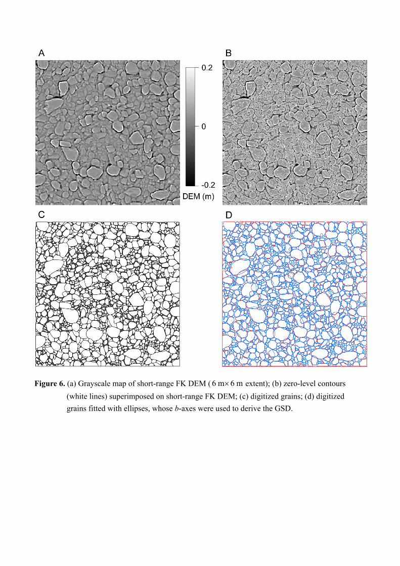
The short-range FK DEM (Fig. 6a) exhibits a grain-scale topographic relief. Individual grains 292

are sharply outlined at the grain boundaries where the residual elevations exhibit a sudden transition 293

from positive values (light gray) to negative values (dark gray). Thus, the zero-level contours of the 294

short-range FK DEM were used in this study as an aid for segmentation of grain boundaries. Figure 295

6b shows the zero-level contours (white lines) of the short-range FK DEM, where individual grains 296

(including many smaller ones) become clearly distinguishable. Some fragmentations associated with 297

grain-surface texture are exhibited also by the zero-level contours. Such textural features on the grain 298

surfaces, however, provide no additional information useful for grain segmentation. 299

Individual grains were digitized manually by a single operator in ArcGIS (Esri) on the hillshade 300

map of OK DEM (as a base map), superimposed with the zero-level contours of the short-range FK 301

DEM (as a visual aid). A total of 1469 grains were recognized and digitized (Fig. 6c), which were 302

fitted with ellipses (Fig. 6d) and their b-axes were used to derive the GSD (Bunte and Abt, 2001), as 303

shown in Fig. 7. The grain sizes range from 27.6 to 569.6 mm with a median size 50D 91 mm. The 304

13

GSD of the digitized grains is well approximated by a lognormal distribution (Fig. 7). 305

Although grain segmentation was done manually in this study, automation of the procedure is 306

possible. The grain segmentation procedure of existing automated grain-sizing software, such as 307

Digital Gravelometer (Graham et al., 2005) and BASEGRAIN (Detert and Weitbrecht, 2012, 2013), 308

can be typically divided into three processes: (1) morphological filtering to enhance grain boundaries 309

or interstices between grains (e.g., bottom-hat transformation); (2) detection of grain boundaries (e.g., 310

edge detection algorithms, double-threshold approach); (3) segmentation of individual grains (e.g., 311

dilation/skeletonization procedure, watershed segmentation). Among these processes, the second is 312

particularly demanding given the difficulty of accurately detecting grain boundaries. Our experience 313

with these automated grain-sizing software indicated that segmentation of individual grains with full 314

automation remains a challenge. With the zero-level contours of the short-range FK DEM usable as a 315

guide to delineate grain boundaries, it is possible to streamline the workflow of grain segmentation 316

by incorporating the zero-level contours into, e.g., the algorithm of automated image segmentation 317

recently devised by Karunatillake et al. (2014) for granulometry and sedimentology. 318

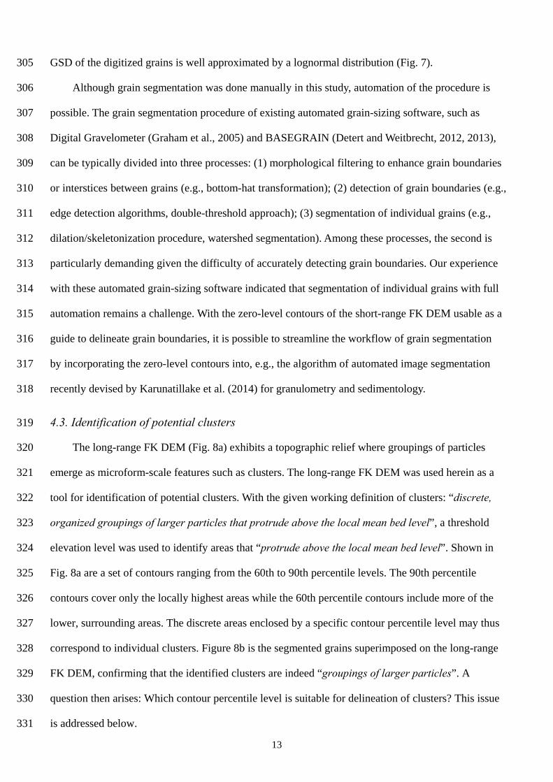
4.3. Identification of potential clusters 319

The long-range FK DEM (Fig. 8a) exhibits a topographic relief where groupings of particles 320

emerge as microform-scale features such as clusters. The long-range FK DEM was used herein as a 321

tool for identification of potential clusters. With the given working definition of clusters: “discrete, 322

organized groupings of larger particles that protrude above the local mean bed level”, a threshold 323

elevation level was used to identify areas that “protrude above the local mean bed level”. Shown in 324

Fig. 8a are a set of contours ranging from the 60th to 90th percentile levels. The 90th percentile 325

contours cover only the locally highest areas while the 60th percentile contours include more of the 326

lower, surrounding areas. The discrete areas enclosed by a specific contour percentile level may thus 327

correspond to individual clusters. Figure 8b is the segmented grains superimposed on the long-range 328

FK DEM, confirming that the identified clusters are indeed “groupings of larger particles”. A 329

question then arises: Which contour percentile level is suitable for delineation of clusters? This issue 330

is addressed below. 331

14

4.4. Delineation of individual clusters 332

To illustrate how individual clusters were delineated, we show in Fig. 8c the discrete areas 333

enclosed by the 60th percentile contours. The segmented grains were superimposed on the enclosed 334

areas, and only those grains that overlapped fully or partially with the enclosed areas were retained. 335

The retained particles were examined for their connectedness. Grains that were mutually connected 336

(or in contact) were grouped into a cluster. This geoprocessing task can be done by Python scripting 337

and automation in ArcGIS. Five clusters so delineated (numbered as 1 to 5) are shown in Fig. 8c, 338

where the constituent grains of a cluster were filled with the same color. 339

In Fig. 8c, the uncolored grains that overlapped with the contour-enclosed areas but were not 340

classified as clusters were eliminated for not meeting the specified minimum number of constituent 341

grains. Herein, to ensure that the delineated clusters are “organized groupings of larger grains”, we 342

adopted a criterion: a cluster consists of at least three abutting grains. By setting the minimum 343

number of constituent grains as three, we aimed to exclude the possibility of unorganized, random 344

groupings. We did not specify a threshold size for anchor clast (referring to the largest grain of a 345

cluster). However, by adopting three as the minimum number of constituent grains, the resulting 346

anchor clasts would be consistently greater than the D90 of the GSD (see Section 5.1). 347

As shown in Fig. 8c, using the 60th percentile contours to identify and delineate potential 348

clusters would result in oversized (or overconnected) clusters. As a result, cluster 2 alone has an area 349

of 14.2 m2, which is nearly 40% of the patch. The total area of these five clusters (= 19.5 m2) exceeds 350

54% of the patch, far greater than the reported values, which rarely exceeded 40% (e.g., Brayshaw, 351

1984; Wittenberg, 2002; Wittenberg and Newson, 2005; Strom and Papanicolaou, 2008; Hendrick et 352

al., 2010). In addition, the length and width of cluster 2 exceed the microform scale (~1 m) revealed 353

by the variogram profile (described in Section 4.1). Clearly, the 60th percentile contours are too low 354

to be a suitable level for delineation of clusters. In the following section, a set of contours ranging 355

from the 70th to 90th percentile levels are used to identify and delineate clusters. The results are 356

compared with a compilation of existing field data, their implications for practical applications are 357

also discussed. 358

15

5. Results and discussion 359

5.1. Delineated clusters 360

Figure 9 shows the delineated clusters resulting from the 70th to 90th percentile contours, with 361

the statistics summarized in Table 1. With increasing contour percentile level, the number of clusters 362

decreases monotonically from 16 to 4, and the corresponding total area of clusters also decreases 363

from 36.6 to 9.1% of the patch (Fig. 9f). The number of constituent grains in each cluster exhibits the 364

widest range of variation (3 to 52 grains) for the 70th percentile contour. Such range of variation 365

reduces with increasing contour percentile level, exhibiting the narrowest range (3 to 18 grains) for 366

the 90th percentile contour. The average number of grains per cluster and average area of individual 367

clusters, however, do not exhibit any monotonic trends with increasing contour percentile level 368

(Table 1), varying in the ranges from 8 to 14 grains/cluster and 0.69 to 0.86 m2/cluster. 369

Despite the lack of monotonic trends in the average number of grains per cluster and mean area 370

per cluster, the mean grain size of clusters increases monotonically from 1.16 to 1.48 times the D90 371

with increasing contour percentile level (Fig. 9f). Coarsening of clusters is observable in Figs. 9a-9e, 372

where the smaller, lower grains surrounding the larger clasts are increasingly excluded with the 373

increase of contour percentile level. Coarsening of clusters is also reflected by the average size of 374

anchor clasts, which increases from 1.8 to 2.18 times the D90 with increasing contour percentile level 375

(Fig. 9f). Variation of anchor size has the widest range for the 70th percentile contour (1.14 to 2.48 376

times the D90) and the narrowest range for the 90th percentile contour (1.99 to 2.48 times the D90). 377

Coarsening of clusters with increasing contour percentile level indicates that a higher delineation 378

standard tends to exclude those smaller, surrounding grains while retaining the larger and more 379

protruding, core particles. 380

A striking feature of our approach is that, even though a criterion for threshold anchor size was 381

not specified, the delineated clusters would always contain an anchor clast that is greater than the D90 382

of the GSD (Table 1). This is in contrast to the conventional approaches for cluster identification, 383

which identify a group of abutting particles that has an anchor clast larger than the specified 384

threshold size, and then verify the identified cluster by examining whether it protrudes above the 385

16

surrounding bed surface (e.g., Oldmeadow and Church, 2006; Hendrick et al., 2010). The use of a 386

threshold anchor size as the primary criterion for cluster identification and a bed topography as the 387

secondary criterion is probably attributable to the fact that grain sizes are more accessible than a 388

detailed DEM. With the support of the FK DEM, however, the delineated clusters not only protrude 389

higher above the bed but also meet the expectation for anchor sizes. Our results thus point towards 390

employing a DEM-based approach rather than a grain-size-based approach for cluster delineation. 391

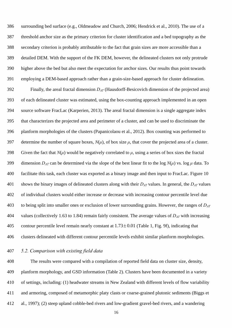
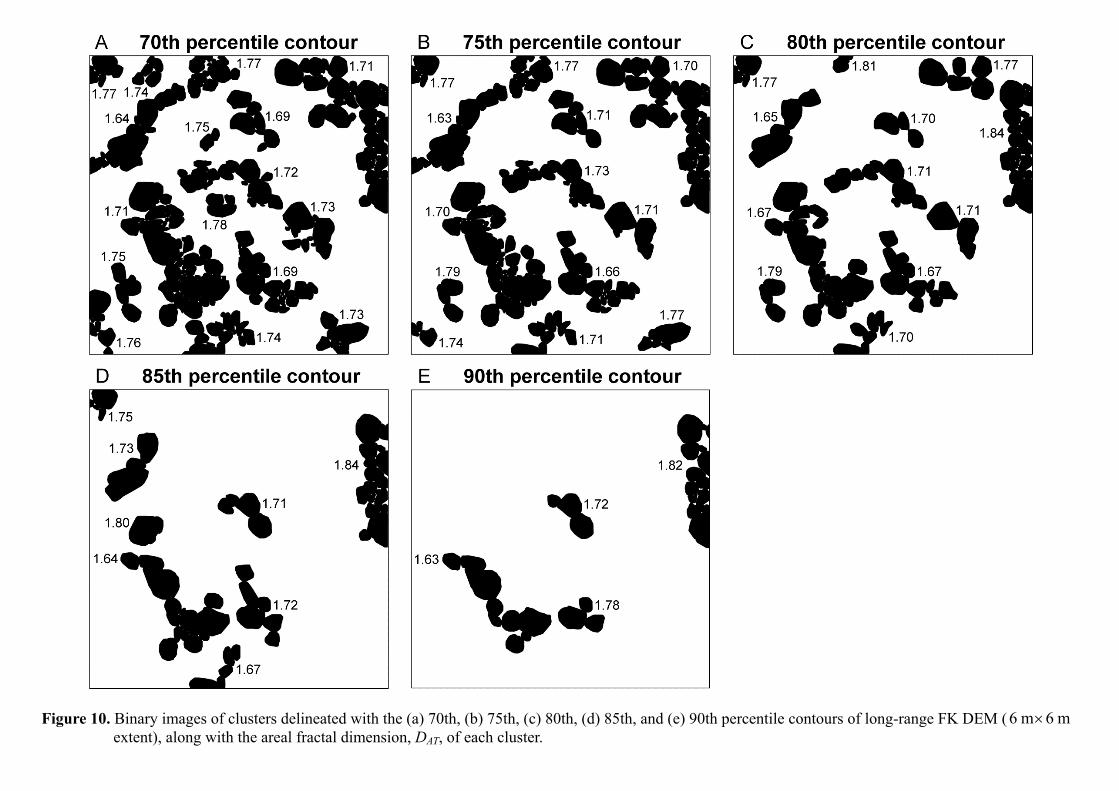
Finally, the areal fractal dimension DAT (Hausdorff-Besicovich dimension of the projected area) 392

of each delineated cluster was estimated, using the box-counting approach implemented in an open 393

source software FracLac (Karperien, 2013). The areal fractal dimension is a single aggregate index 394

that characterizes the projected area and perimeter of a cluster, and can be used to discriminate the 395

planform morphologies of the clusters (Papanicolaou et al., 2012). Box counting was performed to 396

determine the number of square boxes, N(μ), of box size μ, that cover the projected area of a cluster. 397

Given the fact that N(μ) would be negatively correlated to μ, using a series of box sizes the fractal 398

dimension DAT can be determined via the slope of the best linear fit to the log N(μ) vs. log μ data. To 399

facilitate this task, each cluster was exported as a binary image and then input to FracLac. Figure 10 400

shows the binary images of delineated clusters along with their DAT values. In general, the DAT values 401

of individual clusters would either increase or decrease with increasing contour percentile level due 402

to being split into smaller ones or exclusion of lower surrounding grains. However, the ranges of DAT 403

values (collectively 1.63 to 1.84) remain fairly consistent. The average values of DAT with increasing 404

contour percentile level remain nearly constant at 1.73 0.01 (Table 1, Fig. 9f), indicating that 405

clusters delineated with different contour percentile levels exhibit similar planform morphologies. 406

5.2. Comparison with existing field data 407

The results were compared with a compilation of reported field data on cluster size, density, 408

planform morphology, and GSD information (Table 2). Clusters have been documented in a variety 409

of settings, including: (1) headwater streams in New Zealand with different levels of flow variability 410

and armoring, composed of metamorphic platy clasts or coarse-grained plutonic sediments (Biggs et 411

al., 1997); (2) steep upland cobble-bed rivers and low-gradient gravel-bed rivers, and a wandering 412

17

gravel-bed river in England (Wittenberg and Newson, 2005; Wittenberg et al., 2007); (3) small, 413

perennial streams in England with well-rounded cobble beds or flint-gravel beds, and upland streams 414

in Wales with slate gravel/cobble beds, all characterized by flashy runoff due to rainfall (Brayshaw, 415

1984, 1985); (4) ephemeral gravel-bed streams in Israel with relatively rare, annual flow events that 416

follow intense rainstorms (Wittenberg, 2002; Wittenberg et al., 2007); (5) Mediterranean gravel-bed 417

rivers in Italy characterized by deeply-incised valleys, poorly-sorted beds and flashy peak flows that 418

occur in autumn (Brayshaw, 1985); (6) typical mountain gravel-bed rivers in USA with pool-riffle 419

morphologies, flowing through steeply-sided glacial valleys, with runoff dominated by snowmelt or 420

affected also by flash floods following rain-on-snow events or intense summer thunderstorms (Strom 421

and Papanicolaou, 2008; Hendrick et al., 2010; Papanicolaou et al., 2012); (7) a mountain stream in a 422

volcanic terrain in the USA, with its plane bed composed of well-sorted cobbles/pebbles and the flow 423

regime dominated by snowmelt (de Jong, 1995); (8) an anthropogenically influenced, small 424

headwater stream in Canada, with step-pool sequences present at the upstream side of a culvert and 425

an armored reach developing downstream of the culvert (Oldmeadow and Church, 2006). Our results 426

add data for a different geographic region. Further background about the settings of these reported 427

sites can be found in the Supplementary file. 428

The attributes compared include grain sizes, sorting indices, cluster density, area percentage, 429

and size of anchor clast (Table 2). Our characteristic sizes ( 50 84 90, , D D D 91, 190, 233 mm) are well 430

within the grain size ranges reported, among which the sediments of the upland cobble-bed rivers in 431

England are the coarsest whereas those of the low-gradient gravel-bed rivers in England are the finest. 432

Our sorting indices, and I SI 0.83 and 1.83, indicating a moderately sorted river reach, resemble 433

those of the armored East Creek in British Columbia, Canada. 434

Our cluster densities range from 0.11 to 0.44 clusters/m2, which are within the reported lower 435

bound values (headwater streams, New Zealand) and upper bound values (Entiat River, USA). The 436

wide range of cluster densities documented in these sites is attributable to differences in flow 437

variability, armoring and grain shape, the criteria adopted to define clusters, and the clustered bars 438

selected for sampling (Biggs et al., 1997; Hendrick et al., 2010). Our proportions of cluster area 439

18

range from 9.1 to 36.6%, which are within the lower bound values associated with the headwater 440

streams (New Zealand) and upper bound values associated with the poorly-sorted, perennial streams 441

(England). The sizes of anchor clasts were scaled by the D84 in a number of datasets compiled, with 442

the lower bound values observed in East Creek (Canada) and upper bound values observed in 443

headwater streams (New Zealand). As mentioned earlier, our anchor sizes range from 1.14 to 2.48 444

times the D90 (equivalent to 1.4 to 3.04 times the D84), which are concordant with the reported range. 445

In particular, our anchor sizes resemble those documented in the wandering River South Tyne (UK). 446

Such resemblance may be attributed to their similarities in sorting indices SI and transport 447

mechanisms. Clusters at our study site and South Tyne were both sampled from a dynamic 448

equilibrium bar that is exposed during low flows but inundated and subjected to active transport 449

during flashy high flow events. Flow direction at the South Tyne study site varies with the stage. 450

Low flows run along the chute or diagonally across the bar, whereas high flows run directly 451

downstream, normal to the chute. This is similar to the stage-dependent variation of transport 452

direction at our study site on a point bar along a channel bend (Clayton and Pitlick, 2007). 453

The work of Papanicolaou et al. (2012) was the only one that documented fractal dimensions of 454

field clusters, which included four line clusters, four triangle clusters, and four rhombic clusters 455

recorded in a mountain gravel-bed stream (American River, USA). Their average values of DAT for 456

line, triangle, and rhombic clusters are 1.62, 1.77, and 1.76, respectively. Our average values of DAT, 457

ranging from 1.72 to 1.74, are similar to their results. The DAT values of individual clusters shown in 458

Fig. 10 also coincide with their findings, where the pseudo-line clusters on the upper left side of Figs. 459

10a-10c exhibit the lowest values of ( 1.64 0.01)ATD , while the mega clusters on the upper right 460

side of Figs. 10c-10e (with the border cropped) exhibit the highest values of ( 1.83 0.01)ATD . 461

As our results fall within the ranges of reported field data, we can conclude that the FK DEM 462

provides a novel, promising tool for cluster delineation. Currently there is no universally accepted 463

definition of clusters, hence to recommend a standard contour percentile level for delineation of 464

clusters may not be practical. Nonetheless, lower levels (e.g., 70th-75th percentile contour) may be 465

used if more of the smaller, surrounding grains are to be included. By contrast, higher levels (e.g., 466

19

80th-85th percentile contour) may be used if only those larger and more protruding, core particles are 467

to be retained. In the absence of benchmark surfaces with correctly delineated clusters together with 468

a unique definition for clusters, delineation of clusters will inevitably remain subjective in nature. 469

Given that clusters vary in their constituent grains, sizes and shapes across environments, however, 470

the parameters used in the FK, i.e., ( )h , 1 2( ) and ( )h h , can be objectively determined from the 471

DEM-based variogram models. 472

Finally, it is deemed intuitive to examine the delineated clusters by 3D visualization, because it 473

would be helpful to have a real sense of what field scientists would see on site. The color patterns of 474

delineated clusters (Figs. 9a-9e) were superimposed on the hillshade map of OK DEM in ArcScene 475

(Esri), and exported as oblique-perspective, stereoscopic images. Figure 11 presents the resulting 476

images of clusters delineated with the 70th, 80th, and 90th percentile contour levels. As mentioned 477

earlier, with increasing contour percentile level the lower, smaller grains surrounding the higher, 478

larger clasts are increasingly excluded, leaving only the more protruding core particles. Since our 479

approach is based on DEMs rather than grain sizes, it may exclude some of the largest but isolated 480

clasts that are not connected or in contact with at least two sufficiently high grains to meet the 481

definition of a cluster. These largest but isolated clasts could otherwise be classified as a cluster if the 482

required minimum number of constituent grains is lowered as two, or a small separation distance is 483

specified allowing for closely neighboring particles to be effectively identified as abutting ones. 484

6. Conclusions 485

In this study, we used the FK to decompose the short- and long-range (grain- and microform- 486

scale) DEMs. The parameters used in the FK were determined from the nested variogram models 487

derived from the OK DEM. The short-range FK DEM was used as an aid for grain segmentation. 488

The contour percentile levels of the long-range FK DEM were used to identify potential clusters. 489

Individual clusters were delineated on the basis of the segmented grains and identified clusters. 490

Our results reveal that the density and total area of delineated clusters decrease with increasing 491

contour percentile level, while the mean grain size of clusters and average anchor size increase with 492

20

the contour percentile level. These results support the observation that larger grains group as clusters 493

and protrude higher above the bed than other smaller grains. The average areal fractal dimension of 494

clusters shows that clusters resulting from different contour percentile levels exhibit similar planform 495

morphologies. A striking feature of the delineated clusters is that anchor clasts are invariably greater 496

than the D90 even though a threshold anchor size is not adopted herein. Comparisons with existing 497

field data show consistency with the observed cluster attributes. Our results thus point toward a 498

promising DEM-based approach for characterizing sediment structures in gravel-bed rivers. 499

Delineation of clusters is important in river science because clusters affect the flowfield near the 500

bed, change the bed structure and are significant controls on sediment transport and thus bed stability 501

(e.g., Robert et al., 1996; Church et al., 1998; Curran and Tan, 2014b). Essential attributes such as the 502

spatial pattern, density, area coverage, and dimensions may be extracted from the delineated clusters. 503

Moreover, isolating roughness scales of gravel-bed topography is increasingly applied in studies of 504

surface processes such as armoring (Powell et al., 2016; Bertin et al., 2017). With grain boundaries 505

segmented and clusters delineated, isolation of grain and microform DEMs could be performed on an 506

individual grain or cluster basis, which could potentially provide further insights into the roughness 507

parameterization. 508

Automation of our approach would be a direction for future efforts. With the zero-level contours 509

of the short-range FK DEM usable as an aid to delineate grain boundaries, it is possible to streamline 510

the workflow by integrating novel algorithms of automated grain segmentation for cluster delineation. 511

In addition, as possible areas for improvement, omni-directional variogram may be replaced by 2D 512

variogram surface to devise a novel, directional FK. The minimum number of constituent grains 513

required for a cluster may be adjusted, and a small separation distance may be specified allowing for 514

closely neighboring grains, particularly some of those largest but isolated clasts, to be effectively 515

identified as abutting ones. 516

Acknowledgments 517

This work was supported by the Ministry of Science and Technology, Taiwan (MOST), granted 518

to FCW (102-2221-E-002-122-MY3, 103-2221-E-002-146-MY3, and 106-2221-E-002 -074 -MY3). 519

21

We appreciate Jordan Clayton, an anonymous reviewer, and Scott Lecce for thoughtful feedback that 520

improved the manuscript. 521

References 522

Aberle, J., Nikora, V., 2006. Statistical properties of armored gravel bed surfaces. Water Resour. Res. 523

42. https://doi.org/10.1029/2005WR004674 524

Alary, C., Demougeot-Renard, H., 2010. Factorial Kriging Analysis as a tool for explaining the 525

complex spatial distribution of metals in sediments. Environ. Sci. Technol. 44, 593–599. 526

https://doi.org/10.1021/es9022305 527

Allaire, S.E., Lange, S.F., Lafond, J.A., Pelletier, B., Cambouris, A.N., Dutilleul, P., 2012. Multiscale 528

spatial variability of CO2 emissions and correlations with physico-chemical soil properties. 529

Geoderma 170, 251–260. https://doi.org/10.1016/j.geoderma.2011.11.019 530

Atkinson, P.M., 2004. Resolution Manipulation and Sub-Pixel Mapping. In: de Jong, S.M., van der 531

Meer, F.D. (Eds.), Remote Sensing Image Analysis: Including the Spatial Domain. Springer, pp. 532

51-70. 533

Bertin, S., Groom, J., Friedrich, H., 2017. Isolating roughness scales of gravel-bed patches. Water 534

Resour. Res. 53, 6841–6856. https://doi.org/10.1002/2016WR020205 535

Biggs, B.J.F., Duncan, M.J., Francoeur, S.N., Meyer, W.D., 1997. Physical characterisation of 536

microform bed cluster refugia in 12 headwater streams, New Zealand. New Zeal. J. Mar. 537

Freshw. Res. 31, 413–422. https://doi.org/10.1080/00288330.1997.9516775 538

Billi, P., 1988. A note on cluster bedform behaviour in a gravel-bed river. Catena 15, 473–481. 539

https://doi.org/10.1016/0341-8162(88)90065-3 540

Bocchi, S., Castrignanò, A., Fornaro, F., Maggiore, T., 2000. Application of factorial kriging for 541

mapping soil variation at field scale. Eur. J. Agron. 13, 295–308. 542

https://doi.org/10.1016/S1161-0301(00)00061-7 543

Bourennane, H., Hinschberger, F., Chartin, C., Salvador-Blanes, S., 2017. Spatial filtering of 544

electrical resistivity and slope intensity: Enhancement of spatial estimates of a soil property. J. 545

Appl. Geophys. 138, 210–219. https://doi.org/10.1016/j.jappgeo.2017.01.032 546

Brasington, J., Vericat, D., Rychkov, I., 2012. Modeling river bed morphology, roughness, and 547

surface sedimentology using high resolution terrestrial laser scanning. Water Resour. Res. 48. 548

https://doi.org/10.1029/2012WR012223 549

Brayshaw, A.C., 1984. Characteristics and origin of cluster bedforms in coarse-grained alluvial 550

channels. In: Koster, E.H., Steel, R.J. (Eds.), Sedimentology of Gravels and Conglomerates, 551

Can. Soc. Petrol. Geol., 77-85. 552

Brayshaw, A.C., 1985. Bed microtopography and entrainment thresholds in gravel-bed rivers. Geol. 553

Soc. Am. Bull. https://doi.org/10.1130/0016-7606(1985)96<218:BMAETI>2.0.CO 554

22

Brayshaw, A.C., Frostick, L.E., Reid, I., 1983. The hydrodynamics of particle clusters and sediment 555

entrapment in coarse alluvial channels. Sedimentology 30, 137–143. 556

https://doi.org/10.1111/j.1365-3091.1983.tb00656.x 557

Buffin-Bélanger, T., Roy, A.G., 1998. Effects of a pebble cluster on the turbulent structure of a 558

depth-limited flow in a gravel-bed river. Geomorphology 25, 249–267. 559

https://doi.org/10.1016/S0169-555X(98)00062-2 560

Bunte, K., Abt, S.R., 2001. Sampling surface and subsurface particle-size distributions in wadable 561

gravel- and cobble-bed streams for analysis in sediment transport, hydraulics, and streambed 562

monitoring. General Technical Report RMRS-GTR-74. USDA Forest Service, Rocky 563

Mountain Research Station, Fort Collins, CO. 428 p. 564

Butler, J.B., Lane, S.N., Chandler, J.H., 2001. Characterization of the Structure of River-Bed Gravels 565

Using Two-Dimensional Fractal Analysis. Math. Geol. 33, 301–330. 566

https://doi.org/10.1023/a:1007686206695 567

Castrignanò, A., Giugliarini, L., Risaliti, R., Martinelli, N., 2000. Study of spatial relationships 568

among some soil physico-chemical properties of a field in central Italy using multivariate 569

geostatistics. Geoderma 97, 39–60. https://doi.org/10.1016/S0016-7061(00)00025-2 570

Church, M., Hassan, M.A., Wolcott, J.F., 1998. Stabilizing self-organized structures in gravel-bed 571

stream channels: Field and experimental observations. Water Resour. Res. 34, 3169–3179. 572

https://doi.org/10.1029/98WR00484 573

Clayton, J.A., Pitlick, J., 2007. Spatial and temporal variations in bed load transport intensity in a 574

gravel bed river bend. Water Resour. Res. 43. https://doi.org/10.1029/2006WR005253 575

Clifford, N.J., Robert, A., Richards, K.S., 1992. Estimation of flow resistance in gravelbedded 576

rivers: a physical explanation of the multiplier of roughness length. Earth Surf. Process. 577

Landforms 17, 111–126. https://doi.org/10.1002/esp.3290170202 578

Cooper, J.R., Tait, S.J., 2009. Water-worked gravel beds in laboratory flumes - A natural analogue? 579

Earth Surf. Process. Landforms 34, 384–397. https://doi.org/10.1002/esp.1743 580

Curran, J.C., Tan, L., 2014a. The effect of cluster morphology on the turbulent flows over an 581

armored gravel bed surface. J. Hydro-Environment Res. 8, 129–142. 582

https://doi.org/10.1016/j.jher.2013.11.002 583

Curran, J.C., Tan, L., 2014b. Effect of bed sand content on the turbulent flows associated with 584

clusters on an armored gravel bed surface. J. Hydraul. Eng. 140, 137–148. 585

https://doi.org/10.1061/(ASCE)HY.1943-7900.0000810 586

Curran, J.C., Waters, K.A., 2014. The importance of bed sediment sand content for the structure of a 587

static armor layer in a gravel bed river. J. Geophys. Res. Earth Surf. 119, 1484–1497. 588

https://doi.org/10.1002/2014JF003143 589

de Jong, C., 1995. Temporal and spatial interactions between river bed roughness, geometry, bedload 590

transport and flow hydraulics in mountain streams – examples from Squaw Creek, Montana 591

23

(USA) and Schmiedlaine/Lainbach (Upper Germany). Berliner Geographische Abhandlungen, 592

59, 229. 593

de Jong, C., Ergenzinger, P., 1995. The interrelations between mountain valley form and river-bed 594

arrangement. In: Hickin (Ed.), River Geomorphology. Wiley, Chichester. pp. 55–91. 595

Detert, M., Weitbrecht, V., 2012. Automatic object detection to analyze the geometry of gravel 596

grains – A free stand-alone tool. In: River Flow 2012. Taylor & Francis, London, pp. 595–600. 597

Detert, M., Weitbrecht, V., 2013. User guide to gravelometric image analysis by BASEGRAIN. In: 598

Fukuoka et al. (Eds.), Advances in River Sediment Research, Taylor & Francis, London. pp. 599

1789-1796. http://www.basement.ethz.ch/download/tools/basegrain.html (Jan. 2018) 600

Dietrich, W.E., Smith, J.D., 1984. Bed load transport in a river meander. Water Resour. Res. 20, 601

1355–1380. https://doi.org/10.1029/WR020i010p01355 602

Dobermann, A., Goovaerts, P., Neue, H.U., 1997. Scale-dependent correlations among soil properties 603

in two tropical lowland rice fields. Soil Sci. Soc. Am. J. 61, 1483–1496. 604

Dubrule, O., 2003. Geostatistics for Seismic Data Integration in Earth Models. Distinguished 605

Instructor Series, No. 6. Society of Exploration Geophysicists, Tulsa, OK, USA. 606

Entwistle, N.S., Heritage, G.L., Johnson, K., 2008. Cluster detection and development using 607

terrestrial laser scanning. Geophysical Research Abstracts, 10, EGU2008-A-03497. EGU 608

General Assembly. 609

Folk, R.L., Ward, W.C., 1957. Brazos River bar, a study in the significance of grain size parameters. J. 610

Sediment. Res. 27, 3–26. https://doi.org/10.1306/74D70646-2B21-11D7-8648000102C1865D 611

Furbish, D.J., 1987. Conditions for geometric similarity of coarse stream-bed roughness. Math. Geol. 612

19, 291–307. https://doi.org/10.1007/BF00897840 613

Galli, A., Gerdil-Neuillet, F., Dadou, C., 1984. Factorial kriging analysis: a substitute to spectral 614

analysis of magnetic data. In: Verly et al. (Eds.), Geostatistics for Natural Resources 615

Characterization. Reidel, Dordrecht, Netherlands, 543-557. 616

Goovaerts, P., 1997. Geostatistics for Natural Resources Evaluation. Oxford University Press, Oxford, 617

UK. 483 p. 618

Goovaerts, P., Webster, R., 1994. Scaledependent correlation between topsoil copper and cobalt 619

concentrations in Scotland. Eur. J. Soil Sci. 45, 79–95. 620

https://doi.org/10.1111/j.1365-2389.1994.tb00489.x 621

Goovaerts, P., Sonnet, P., Navarre, A., 1993. Factorial kriging analysis of springwater contents in the 622

Dyle River Basin, Belgium. Water Resour. Res. 29, 2115–2125. 623

https://doi.org/10.1029/93WR00588 624

Goovaerts, P., Jacquez, G.M., Marcus, A., 2005a. Geostatistical and local cluster analysis of high 625

resolution hyperspectral imagery for detection of anomalies. Remote Sens. Environ. 95, 626

351–367. https://doi.org/10.1016/j.rse.2004.12.021 627

Goovaerts, P., Jacquez, G.M., Greiling, D., 2005b. Exploring scale-dependent correlations between 628

24

cancer mortality rates using factorial kriging and population-weighted semivariograms. Geogr. 629

Anal. 37, 152–182. https://doi.org/10.1111/j.1538-4632.2005.00634.x 630

Graham, D.J., Reid, I., Rice, S.P., 2005. Automated sizing of coarse-grained sediments: 631

Image-processing procedures. Math. Geol. 37, 1–28. http://www.sedimetrics.com (Jan. 2018) 632

Hardy, R.J., Best, J.L., Lane, S.N., Carbonneau, P.E., 2009. Coherent flow structures in a 633

depth-limited flow over a gravel surface: the role of near-bed turbulence and influence of 634

Reynolds number. J. Geophys. Res. Earth Surf. 114. https://doi.org/10.1029/2007JF000970 635

Hassan, M.A., Reid, I., 1990. The influence of microform bed roughness elements on flow and 636

sediment transport in gravel bed rivers. Earth Surf. Proc. Land. 15, 739-750. 637

Hassan, M.A., Church, M., 2000. Experiments on surface structure and partial sediment transport on 638

a gravel bed. Water Resour. Res. 36, 1885–1895. https://doi.org/10.1029/2000WR900055 639

Hassan, M.A., Smith, B.J., Hogan, D.L., Luzi, D.S., Zimmermann, A.E., Eaton, B.C., 2008. 640

Sediment storage and transport in coarse bed streams: scale considerations. In: Habersack et al. 641

(Eds.), Gravel-Bed Rivers VI: From Process Understanding to River Restoration. Elsevier, 642

Amsterdam, Netherland, pp. 473-496. 643

Heays, K.G., Friedrich, H., Melville, B.W., 2014. Laboratory study of gravel-bed cluster formation 644

and disintegration. Water Resour. Res. 50, 2227–2241. https://doi.org/10.1002/2013WR014208 645

Hendrick, R.R., Ely, L.L., Papanicolaou, A.N., 2010. The role of hydrologic processes and 646

geomorphology on the morphology and evolution of sediment clusters in gravel-bed rivers. 647

Geomorphology 114, 483–496. https://doi.org/10.1016/j.geomorph.2009.07.018 648

Hodge, R., Brasington, J., Richards, K., 2009. Analysing laser-scanned digital terrain models of 649

gravel bed surfaces: linking morphology to sediment transport processes and hydraulics. 650

Sedimentology 56, 2024–2043. https://doi.org/10.1111/j.1365-3091.2009.01068.x 651

Hodge, R.A., 2010. Using simulated Terrestrial Laser Scanning to analyse errors in high-resolution 652

scan data of irregular surfaces. ISPRS J. Photogramm. Remote Sens. 65, 227–240. 653

https://doi.org/10.1016/j.isprsjprs.2010.01.001 654

Huang, G.H., Wang, C.K., 2012. Multiscale geostatistical estimation of gravel-bed roughness from 655

terrestrial and airborne laser scanning. IEEE Geosci. Remote Sens. Lett. 9, 1084–1088. 656

https://doi.org/10.1109/LGRS.2012.2189351 657

Isaaks, E.H., Srivastava, R.M., 1989. An Introduction to Applied Geostatistics. Oxford University 658

Press, New York. 561 p. 659

Jaquet, O., 1989. Factorial kriging analysis applied to geological data from petroleum exploration. 660

Math. Geol. 21, 683–691. https://doi.org/10.1007/BF00893316 661

Journel, A.G., Huijbregts, C.J., 1978. Mining Geostatistics. Academic Press, London. 600 p. 662

Karperien, A., 2013. FracLac for ImageJ. 663

http://rsb.info.nih.gov/ij/plugins/fraclac/FLHelp/Introduction.htm (Jan. 2018) 664

Karunatillake, S., McLennan, S.M., Herkenhoff, K.E., Husch, J.M., Hardgrove, C., Skok, J.R., 2014. 665

25

A martian case study of segmenting images automatically for granulometry and sedimentology, 666

Part 1: Algorithm. Icarus 229, 400–407. https://doi.org/10.1016/j.icarus.2013.10.001 667

Kerry, R., Goovaerts, P., Haining, R.P., Ceccato, V., 2010. Applying geostatistical analysis to crime 668

data: car-related thefts in the Baltic states. Geogr. Anal. 42, 53–77. 669

https://doi.org/10.1111/j.1538-4632.2010.00782.x 670

Lacey, R.W.J., Roy, A.G., 2007. A comparative study of the turbulent flow field with and without a 671

pebble cluster in a gravel bed river. Water Resour. Res. 43. 672

https://doi.org/10.1029/2006WR005027 673

L’Amoreaux, P., Gibson, S., 2013. Quantifying the scale of gravel-bed clusters with spatial statistics. 674

Geomorphology 197, 56–63. https://doi.org/10.1016/j.geomorph.2013.05.002 675

Lawless, M., Robert, A., 2001a. Three-dimensional flow structure around small-scale bedforms in 676

simulated gravel-bed environment. Earth Surf. Process. Landforms 26, 507–522. 677

https://doi.org/10.1002/esp.195 678

Lawless, M., Robert, A., 2001b. Scales of boundary resistance in coarse-grained channels: turbulent 679

velocity profiles and implications. Geomorphology 39, 221–238. 680

https://doi.org/10.1016/S0169-555X(01)00029-0 681

Lv, J., Liu, Y., Zhang, Z., Dai, J., 2013. Factorial kriging and stepwise regression approach to identify 682

environmental factors influencing spatial multi-scale variability of heavy metals in soils. J. 683

Hazard. Mater. 261, 387–397. https://doi.org/10.1016/j.jhazmat.2013.07.065 684

Ma, Y.Z., Royer, J.J., Wang, H., Wang, Y., Zhang, T., 2014. Factorial kriging for multiscale 685

modelling. J. South. African Inst. Min. Metall. 114, 651–657. 686

Mao, L., 2012. The effect of hydrographs on bed load transport and bed sediment spatial 687

arrangement. J. Geophys. Res. Earth Surf. 117. https://doi.org/10.1029/2012JF002428 688

Mao, L., Cooper, J.R., Frostick, L.E., 2011. Grain size and topographical differences between static 689

and mobile armour layers. Earth Surf. Process. Landforms 36, 1321–1334. 690

https://doi.org/10.1002/esp.2156 691

Marion, A., Tait, S.J., McEwan, I.K., 2003. Analysis of small-scale gravel bed topography during 692

armoring. Water Resour. Res. 39. https://doi.org/10.1029/2003WR002367 693

Matheron, G., 1971. The Theory of Regionalized Variables and its Applications. Cahiers du Centre 694

de Morphologie Mathématique, No. 1. Fontainebleau, France. 695

Matheron, G., 1982. Pour une Analyse Krigeante de Données Régionalisées: Note interne, N-732. 696

Centre de Géostatistique, Fontainebleau, France. 22 p. 697

Milan, D., Heritage, G., 2012. LiDAR and ADCP use in gravel-bed rivers: advances since GBR6. In: 698

Church et al. (Eds.), Gravel-Bed Rivers: Processes, Tools, Environments. Wiley, Chichester, 699

UK, pp. 286-302. 700

Nikora, V.I., Goring, D.G., Biggs, B.J.F., 1998. On gravel-bed roughness characterization. Water 701

Resour. Res. 34, 517–527. https://doi.org/10.1029/97WR02886 702

26

Oldmeadow, D.F., Church, M., 2006. A field experiment on streambed stabilization by gravel 703

structures. Geomorphology 78, 335–350. https://doi.org/10.1016/j.geomorph.2006.02.002 704

Oliver, M.A., Webster, R., 1986. Semivariograms for modelling the spatial pattern of landform and 705

soil properties. Earth Surf. Process. Landforms 11, 491–504. 706

https://doi.org/10.1002/esp.3290110504 707

Oliver, M.A., Webster, R., Slocum, K., 2000. Filtering SPOT imagery by kriging analysis. Int. J. 708

Remote Sens. 21, 735–752. https://doi.org/10.1080/014311600210542 709

Paola, C., Seal, R., 1995. Grain size patchiness as a cause of selective deposition and downstream 710

fining. Water Resour. Res. 31, 1395-1407. 711

Papanicolaou, A.N., Strom, K., Schuyler, A., Talebbeydokhti, N., 2003. The role of sediment specific 712

gravity and availability on cluster evolution. Earth Surf. Process. Landforms 28, 69–86. 713

https://doi.org/10.1002/esp.427 714

Papanicolaou, A.N.T., Tsakiris, A.G., Strom, K.B., 2012. The use of fractals to quantify the 715

morphology of cluster microforms. Geomorphology 139–140, 91–108. 716

https://doi.org/10.1016/j.geomorph.2011.10.007 717

Pebesma, E.J., 2004. Multivariable geostatistics in S: the gstat package. Computers & Geosciences 718

30, 683-691. https://cran.r-project.org/package=gstat (Jan. 2018) 719

Piedra, M.M., Haynes, H., Hoey, T.B., 2012. The spatial distribution of coarse surface grains and the 720

stability of gravel river beds. Sedimentology 59, 1014–1029. 721

https://doi.org/10.1111/j.1365-3091.2011.01290.x 722

Powell, D.M., Ockelford, A., Rice, S.P., Hillier, J.K., Nguyen, T., Reid, I., Tate, N.J., Ackerley, D., 723

2016. Structural properties of mobile armors formed at different flow strengths in gravel-bed 724

rivers. J. Geophys. Res. Earth Surf. 121, 1494–1515. https://doi.org/10.1002/2015JF003794 725

Reid, I., Frostick, L.E., Brayshaw, A.C., 1992. Microform roughness elements and the selective 726

entrainment and entrapment of particles in gravel-bed rivers. In: Billi et al. (Eds.), Dynamics of 727

Gravel-Bed Rivers. Wiley, Chichester. 253-276. 728

Reis, A.P., Sousa, A.J., Ferreira Da Silva, E., Patinha, C., Fonseca, E.C., 2004. Combining multiple 729

correspondence analysis with factorial kriging analysis for geochemical mapping of the 730

gold-silver deposit at Marrancos (Portugal). Appl. Geochemistry 19, 623–631. 731

https://doi.org/10.1016/j.apgeochem.2003.09.003 732

Rice, S.P., Buffin-Bélanger, T., Reid, I., 2014. Sensitivity of interfacial hydraulics to the 733

microtopographic roughness of water-lain gravels. Earth Surf. Process. Landforms 39, 184–199. 734

https://doi.org/10.1002/esp.3438 735

Robert, A., 1988. Statistical properties of sediment bed profiles in alluvial channels. Math. Geol. 20, 736

205–225. https://doi.org/10.1007/BF00890254 737

Robert, A., 1991. Fractal properties of simulated bed profiles in coarse-grained channels. Math. Geol. 738

23, 367–382. https://doi.org/10.1007/BF02065788 739

27

Robert, A., Roy, A.G., DeSerres, B., 1996. Turbulence at a roughness transition in a depth limited 740

flow over a gravel bed. Geomorphology 16, 175–187. 741

https://doi.org/10.1016/0169-555X(95)00143-S 742

Sandjivy, L., 1984. The factorial kriging analysis of regionalized data: its application to geochemical 743

prospecting. In: Verly et al. (eds.), Geostatistics for Natural Resources Characterization. Reidel, 744

Dordrecht, Netherlands, pp. 559-571. 745

Smart, G.M., Duncan, M.J., Walsh, J.M., 2002. Relatively rough flow resistance equations. J. 746

Hydraul. Eng. 128, 568–578. https://doi.org/10.1061/(ASCE)0733-9429(2002)128:6(568) 747

Strom, K.B., Papanicolaou, A.N., 2008. Morphological characterization of cluster microforms. 748

Sedimentology 55, 137–153. https://doi.org/10.1111/j.1365-3091.2007.00895.x 749

Strom, K.B., Papanicolaou, A.N., 2009. Occurrence of cluster microforms in mountain rivers. Earth 750

Surf. Process. Landforms 34, 88–98. https://doi.org/10.1002/esp.1693 751

Strom, K., Papanicolaou, A.N., Evangelopoulos, N., Odeh, M., 2004. Microforms in gravel bed 752

rivers: formation, disintegration, and effects on bedload transport. J. Hydraul. Eng. 130, 753

554–567. https://doi.org/10.1061/(ASCE)0733-9429(2004)130:6(554) 754

Strom, K.B., Papanicolaou, A.N., Constantinescu, G., 2007. Flow heterogeneity over 3D cluster 755

microform: laboratory and numerical investigation. J. Hydraul. Eng. 133, 273–287. 756

https://doi.org/10.1061/(ASCE)0733-9429(2007)133:3(273) 757

Van Meirvenne, M., Goovaerts, P., 2002. Accounting for spatial dependence in the processing of 758

multi-temporal SAR images using factorial kriging. Int. J. Remote Sens. 23, 371–387. 759

https://doi.org/10.1080/01431160010014800 760

Wang, C.K., Wu, F.C., Huang, G.H., Lee, C.Y., 2011. Mesoscale terrestrial laser scanning of fluvial 761

gravel surfaces. IEEE Geosci. Remote Sens. Lett. 8, 1075–1079. 762

https://doi.org/10.1109/LGRS.2011.2156758 763

Webster, R, Oliver, M.A., 2007. Geostatistics for Environmental Scientists, 2nd Ed. Wiley, 764

Chichester, 330 p. 765

Wen, R., Sinding-Larsen, R., 1997. Image filtering by factorial kriging—sensitivity analysis and 766

application to Gloria side-scan sonar images. Math. Geol. 29, 433–468. 767

https://doi.org/10.1007/BF02775083 768

Wittenberg, L., 2002. Structural patterns in coarse gravel river beds: typology, survey and assessment 769

of the roles of grain size and river regime. Geogr. Ann. Ser. A-Physical Geogr. 84A, 25–37. 770

https://doi.org/10.1111/j.0435-3676.2002.00159.x 771

Wittenberg, L., Newson, M.D., 2005. Particle clusters in gravel-bed rivers: an experimental 772

morphological approach to bed material transport and stability concepts. Earth Surf. Process. 773

Landforms 30, 1351–1368. https://doi.org/10.1002/esp.1184 774

Wittenberg, L., Laronne, J.B., Newson, M.D., 2007. Bed clusters in humid perennial and 775

Mediterranean ephemeral gravel-bed streams: the effect of clast size and bed material sorting. J. 776

28

Hydrol. 334, 312–318. https://doi.org/10.1016/j.jhydrol.2006.09.028 777

Yao, T., Mukerji, T., Journel, A.G., Mavko, G., 1999. Scale matching with factorial kriging for 778

improved porosity estimation from seismic data. Math. Geol. 31, 23–46. 779

https://doi.org/10.1023/A:1007589213368 780

Figure Captions 781

Fig. 1. A schematic empirical variogram profile (solid circles) that exhibits two scaling regions. Lags 782

between 1[0, ]a correspond to grain-scale structure; lags between 1 2[ , ]a a correspond to 783

microform-scale structure; lags > 2a correspond to saturation region with constant sill. The 784

empirical variogram profile is fitted with a double spherical model (red line) that combines 785

linearly two single spherical models (blue lines), one has a short range 1a , the other has a long 786

range 2a , with 1c and 2c being the corresponding sills. 787

Fig. 2. An example gravel-bed patch collected from Nanshih Creek (northern Taiwan): (a) ordinary 788

kriged (OK) DEM; (b) short-range component of factorial kriged (FK) DEM; (c) long-range 789

component of FK DEM; (d) surface elevation distributions of OK DEM, and short- and 790

long-range FK DEMs. 791

Fig. 3. (a) Orthorectified photograph of the study site (24˚54'10"N, 121˚33'24"E) at a point bar in 792

lower Nanshih Creek (northern Taiwan). Scanned gravel-bed patch is indicated by a square box, 793

flow directions are indicated by arrows. (b) Oblique view of the 6 m 6 m gravel-bed patch, 794

around which a 1 m wide buffer on each side was set with a yellow tape. 795

Fig. 4. (a) Oblique-perspective grayscale intensity image of terrestrial laser scanning (TLS) data. 796

Yellow arrows point at spherical targets (14.5 cm in diameter) used for data co-registration and 797

merge; (b) grayscale map of OK DEM (1 cm 1 cm resolution) of the 6 m 6 m gravel-bed 798

patch; (c) color hillshade map of OK DEM. Red arrows point at the same location toward the 799

same direction. 800

Fig. 5. Omni-directional variograms of the OK DEM: empirical variogram (solid circles) is fitted 801

with a nested double spherical model (gray line) that combines linearly a short-range spherical 802

model (red line) and a long-range spherical model (blue line), with the short and long ranges: 803

1a 0.470 m, 2a 0.962 m, and sills 31 6.457 10c m2, 3

2 4.954 10c m2. 804

Fig. 6. (a) Grayscale map of short-range FK DEM (6 m 6 m extent); (b) zero-level contours (white 805

lines) superimposed on short-range FK DEM; (c) digitized grains; (d) digitized grains fitted 806

with ellipses, whose b-axes were used to derive the GSD. 807

Fig. 7. Grain size distribution (GSD) derived from b-axes of digitized grains (Fig. 6d). The GSD is 808

well approximated by a lognormal distribution. 809

Fig. 8. (a) Color map of long-range FK DEM ( 6 m 6 m extent), superimposed by contours ranging 810

from the 60th to 90th percentile levels; (b) long-range FK DEM superimposed by digitized 811

grains; (c) delineated clusters resulting from the 60th percentile contours (blue lines), where the 812

constituent grains of a cluster are filled with the same color, while the uncolored grains are 813

29

eliminated for not meeting the required minimum number of constituent grains. (See text for 814

details) 815

Fig. 9. Delineated clusters resulting from the (a) 70th, (b) 75th, (c) 80th, (d) 85th, and (e) 90th 816

percentile contours of long-range FK DEM ( 6 m 6 m extent), grains filled with the same 817

colors are the constituent particles of individual clusters, uncolored grains are eliminated ones, 818

and arrows indicate channel centerline directions; (f) summary statistics of cluster attributes. 819

Fig. 10. Binary images of clusters delineated with the (a) 70th, (b) 75th, (c) 80th, (d) 85th, and (e) 820

90th percentile contours of long-range FK DEM (6 m 6 m extent), along with the areal fractal 821

dimension, DAT, of each cluster. 822

Fig. 11. 3D visualization of clusters delineated with the (a) 70th, (b) 80th, and (c) 90th percentile 823

contours of long-range FK DEM, and (d) the same view with no clusters mapped (6 m 6 m824

extent). Arrows indicate channel centerline directions. 825

826

Table 1. Attribute statistics of individual clusters delineated with the 70th to 90th percentile contours of long-range FK DEM

Cluster ID

70th percentile contour 75th percentile contour 80th percentile contour 85th percentile contour 90th percentile contour

No. of grains

Area (m2)

Anchor size (× D90)

DAT No. of grains

Area (m2)

Anchor size(× D90)

DATNo. of grains

Area (m2)


DATNo. of grains

Area (m2)

Anchor size(× D90)

DATNo. of grains

Area (m2)


DAT

1 6 0.28 2.07 1.77 5 0.24 2.07 1.77 5 0.24 2.07 1.77 4 0.21 2.07 1.75 18 1.08 2.26 1.82

2 5 0.23 1.15 1.74 13 0.49 1.81 1.77 3 0.10 1.39 1.81 3 0.65 2.45 1.73 3 0.41 2.01 1.72

3 16 0.53 1.81 1.77 37 2.50 2.26 1.70 5 0.77 2.23 1.77 22 1.24 2.26 1.84 9 1.24 2.48 1.63

4 39 2.56 2.26 1.71 11 1.05 2.45 1.63 4 0.77 2.45 1.65 3 0.40 2.39 1.80 5 0.52 1.99 1.78

5 13 1.08 2.45 1.64 6 0.55 1.82 1.71 3 0.33 1.82 1.70 4 0.47 2.01 1.71

6 3 0.10 1.14 1.75 16 0.89 2.01 1.73 24 1.26 2.26 1.84 16 1.58 2.48 1.64

7 7 0.58 1.82 1.69 3 0.29 1.45 1.79 9 0.80 2.01 1.71 6 0.69 1.99 1.72

8 18 0.94 2.01 1.72 44 2.58 2.48 1.70 3 0.29 1.45 1.79 5 0.30 1.34 1.67

9 52 2.74 2.48 1.71 16 1.04 1.99 1.66 25 2.23 2.48 1.67

10 3 0.23 1.16 1.78 4 0.55 2.39 1.71 11 0.94 1.99 1.67

11 10 0.68 2.39 1.73 3 0.14 1.48 1.74 3 0.53 2.39 1.71

12 5 0.39 1.45 1.75 9 0.48 1.34 1.71 7 0.41 1.34 1.70

13 24 1.30 1.99 1.69 4 0.36 1.74 1.77

14 7 0.38 1.48 1.76

15 16 0.67 1.34 1.74

16 6 0.49 1.74 1.73

Average 14 0.82 1.80 1.73 13 0.86 1.94 1.72 9 0.72 1.99 1.73 8 0.69 2.12 1.73 9 0.81 2.18 1.74

Mean grain size of cluster (× D90)

1.16 1.24 1.41 1.44 1.48

Total area (m2) 13.18 11.17 8.67 5.55 3.26

Area percentage 36.6 31.0 24.1 15.4 9.1

Table 2. Comparison of cluster attributes from this study with those from previous field studies

Attribute This study Previous field studies Sources

Grain sizes

D50 (mm)

91

30 - 97 (11 cobble/gravel bed rivers, NE England)

40 - 105 (American and S.F. Snoqualmie Rivers, USA)

29 - 91 (Entiat River, USA)

Wittenberg et al. (2007)

Strom and Papanicolaou (2008)

Hendrick et al. (2010)

D84 (mm) 190 45 - 215 (12 headwater streams, New Zealand)

45 - 224 (11 cobble/gravel bed rivers, NE England)


50 - 210 (6 cluster-dominated river beds, worldwide)

Biggs et al. (1997)




D90 (mm) 233 104 - 441 (7 rivers, NE England and Mt. Carmel Israel)

55 - 315 (15 rivers, NE England, Mt. Carmel/Negev Israel)

Wittenberg (2002)


Sorting indices 1

I

0.83

0.89 (East Creek, BC Canada)

0.75 - 1.74 (15 rivers, NE England, Mt. Carmel/Negev Israel)

Oldmeadow and Church (2006)


SI

1.83

1.73 - 3.59 (7 rivers, NE England and Mt. Carmel Israel)

1.57 - 2.47 (dynamic equilibrium bar, River South Tyne, UK)


1.72 - 3.11 (11 cobble/gravel bed rivers, NE England)

< 2.4 (American and S.F. Snoqualmie Rivers, USA)

Wittenberg (2002)

Wittenberg and Newson (2005)




Cluster density

(clusters/m2) 0.11 - 0.44

0.07 - 0.28 (12 headwater streams, New Zealand)



0.7 - 1.5 (Entiat River, USA)

Biggs et al. (1997)




Proportion of

cluster area (%)

9.1 - 36.6

5 - 10 (4 gravel-bed rivers, England and Italy)


30 - 40 (4 perennial streams, NE England)

8 - 22 (3 ephemeral streams, Mt. Carmel Israel)

7 - 16 (dynamic equilibrium bar, River South Tyne, UK)

6 - 39 (15 rivers, NE England, Mt. Carmel/Negev Israel)


> 15 (cluster bars, Entiat River, USA)

Brayshaw (1985)

Biggs et al. (1997)

Wittenberg (2002)

Wittenberg (2002)





Size of anchor

clast (× D84)

1.40 - 3.04



1 - 1.66 (East Creek, BC Canada)

> 1.18 - 1.85 (11 cobble/gravel bed rivers, NE England)

1.22 - 1.95 (American and S.F. Snoqualmie Rivers, USA)

Biggs et al. (1997)





Areal fractal

dimension DAT 1.72 - 1.74 1.62 - 1.77 (12 clusters, American River, USA) Papanicolaou et al. (2012)

1 84 16 95 5/ 4 / 6.6I , where 2logi iD ; 84 50 50 16( / / ) / 2SI D D D D .

Figure 1. A schematic empirical variogram profile (solid circles) that exhibits two scaling regions.

Lags between 1[0, ]a correspond to grain-scale structure; lags between 1 2[ , ]a a correspond to

microform-scale structure; lags > 2a correspond to saturation region with constant sill. The

empirical variogram profile is fitted with a double spherical model (red line) that combines

linearly two single spherical models (blue lines), one has a short range 1a , the other has a

long range 2a , with 1c and 2c being the corresponding sills.

Figure 2. An example gravel-bed patch collected from Nanshih Creek (northern Taiwan): (a) ordinary kriged (OK) DEM; (b) short-range component of factorial kriged (FK) DEM; (c) long-range component of FK DEM; (d) surface elevation distributions of OK DEM, and short- and long-range FK DEMs.

Figure 3. (a) Orthorectified photograph of the study site (24˚54'10"N, 121˚33'24"E) at a point bar in

lower Nanshih Creek (northern Taiwan). Scanned gravel-bed patch is indicated by a square

box, flow directions are indicated by arrows. (b) Oblique view of the 6 m 6 m gravel-bed

patch, around which a 1 m wide buffer on each side was set with a yellow tape.

Figure 4. (a) Oblique-perspective grayscale intensity image of terrestrial laser scanning (TLS) data. Yellow arrows point at spherical targets (14.5 cm in diameter)

used for data co-registration and merge; (b) grayscale map of OK DEM (1 cm 1 cm resolution) of the 6 m 6 m gravel-bed patch; (c) color hillshade

map of OK DEM. Red arrows point at the same location toward the same direction.

Figure 5. Omni-directional variograms of the OK DEM: empirical variogram (solid circles) is fitted

with a nested double spherical model (gray line) that combines linearly a short-range

spherical model (red line) and a long-range spherical model (blue line), with the short and

long ranges: 1a 0.470 m, 2a 0.962 m, and sills 31 6.457 10c m2, 3

2 4.954 10c m2.

Figure 6. (a) Grayscale map of short-range FK DEM ( 6 m 6 m extent); (b) zero-level contours

(white lines) superimposed on short-range FK DEM; (c) digitized grains; (d) digitized

grains fitted with ellipses, whose b-axes were used to derive the GSD.

Figure 7. Grain size distribution (GSD) derived from b-axes of digitized grains (Figure 6d). The GSD is well approximated by a lognormal distribution.

Figure 8. (a) Color map of long-range FK DEM ( 6 m 6 m extent), superimposed by contours ranging from the 60th to 90th percentile levels; (b) long-range FK

DEM superimposed by digitized grains; (c) delineated clusters resulting from the 60th percentile contours (blue lines), where the constituent grains of a cluster are filled with the same color, while the uncolored grains are eliminated for not meeting the required minimum number of constituent grains. (See text for details)

Figure 9. Delineated clusters resulting from the (a) 70th, (b) 75th, (c) 80th, (d) 85th, and (e) 90th percentile contours of long-range FK DEM ( 6 m 6 m extent), grains filled with the same colors are the constituent particles of individual clusters, uncolored grains are eliminated ones, and arrows indicate channel centerline directions; (f) summary statistics of cluster attributes.

Figure 10. Binary images of clusters delineated with the (a) 70th, (b) 75th, (c) 80th, (d) 85th, and (e) 90th percentile contours of long-range FK DEM (6 m 6 mextent), along with the areal fractal dimension, DAT, of each cluster.

Figure 11. 3D visualization of clusters delineated with the (a) 70th, (b) 80th, and (c) 90th percentile contours of long-range FK DEM, and (d) the same view with no clusters mapped ( 6 m 6 m extent). Arrows indicate channel centerline directions.

Date post:	22-May-2018
Category:	Documents
Upload:	truongtuyen
View:	222 times
Download:	0 times

Delineation of gravel-bed clusters via factorial kriging 2 ... 1 Delineation of gravel-bed clusters...

Documents