Project SELECT - Smart Efficient Location, idEntification and Cooperation Techniques Project- No 257544 Work Package Identification, location and modelling WP – No WP2 Document Deliverable D2.2.1 SaveDate 05/09/2011 D2.2.1_Signal_processing_techniques_interim_report_1.3_CNIT Dissemination Level: Public Page 1/142 THEME ICT ICT 2009.3.9 Microsystems and Smart Miniaturised Systems ProgrammeTitle Collaborative project / Small or medium-scale focused research projects Project Title Smart Efficient Location, idEntification and Cooperation Techniques Acronym SELECT Project No 257544 DELIVERABLE D2.2.1 Signal processing techniques: Interim report WorkPackage2 Leading Partner: CNIT Document Editor: Davide Dardari (CNIT) Dissemination Level: PU - Public Delivery date: 31/8/2011 Version 1.3
Transcript
Project SELECT - Smart Efficient Location, idEntification and Cooperation Techniques Project- No 257544 Work Package Identification, location and modelling WP – No WP2 Document Deliverable D2.2.1 SaveDate 05/09/2011
D2.2.1_Signal_processing_techniques_interim_report_1.3_CNIT Dissemination Level: Public Page 1/142
THEME ICT
ICT 2009.3.9 Microsystems and Smart Miniaturised Systems
ProgrammeTitle Collaborative project / Small or medium-scale focused research projects
Project Title
Smart Efficient Location, idEntification and Cooperation Techniques Acronym
SELECT Project No
257544
DELIVERABLE D2.2.1
Signal processing techniques: Interim report
WorkPackage2 Leading Partner: CNIT
Document Editor: Davide Dardari (CNIT)
Dissemination Level: PU - Public
Delivery date: 31/8/2011
Version 1.3
Project SELECT - Smart Efficient Location, idEntification and Cooperation Techniques Project- No 257544 Work Package Identification, location and modelling WP – No WP2 Document Deliverable D2.2.1 SaveDate 05/09/2011
D2.2.1_Signal_processing_techniques_interim_report_1.3_CNIT Dissemination Level: Public Page 2/142
Contributors
Partner Contributing authors
DATALOGIC
Fraunhofer
CEA F. Dehmas, V. Heiries, R. D’Errico
CNIT D. Dardari, A. Conti, N. Decarli, S. Bartoletti, V. Casadei, M. Guerra, A. Mariani
CEIT
ARMINES A. Sibille, F. Guidi
NOV
ORIA
Versioning and contribution history
Version Description Contributing authors Date
0.1 TOC D. Dardari 8/3/2011 0.2 Sections
1,2,5,6.1 S. Bartoletti, V. Casadei, A. Conti, R. D’Errico, D. Dardari, N. Decarli, F. Dehmas, M. Guerra, F. Guidi, V. Heiries, A. Mariani
9/5/2011
0.3 Editing D. Dardari – A. Conti – N. Decarli 17/5/2011 0.4 Editing, section
6.2 N. Decarli, V. Heiries 25/6/2011
1.0 Editing D. Dardari 1/7/2011 Internal review M. Bottazzi, G. Micheletti, D. Wisland 1.1 Review A. Conti, D. Dardari 29/8/2011 1.2 Final Review A. Conti, V. Heiries 31/8/2011 1.3 Final Re-format M.Bottazzi 31/8/2011
Project SELECT - Smart Efficient Location, idEntification and Cooperation Techniques Project- No 257544 Work Package Identification, location and modelling WP – No WP2 Document Deliverable D2.2.1 SaveDate 05/09/2011
D2.2.1_Signal_processing_techniques_interim_report_1.3_CNIT Dissemination Level: Public Page 3/142
LIST OF ACRONYMS
Acronym Name
ADC Analog to Digital Converter
AWGN Addictive White Gaussian Noise
BAV Balanced Antipodal Vivaldi
BEP Bit Error Probability
BER Bit Error Rate
BWA Broadband Wireless Access
CAF Cyclic Autocorrelation Function
CIR Channel Impulse Response
CM Channel Model
CP Cyclic Prefix
CPAPR Cross-correlation Peak to Autocorrelation Peak Ratio
CPGPR Cross-correlation Peak to Grass Peak Ratio
CRLB Cramer-Rao Lower Bound
CSCG Circularly Symmetric Complex Gaussian
CW Continuous Wave
DAA Detect And Avoid
DAC Digital to Analog Converter
DFMS Monopole Dual Feed Stripline Antenna
ED Energy Detector
EFIM Equivalent Fisher Information Matrix
EIRP Equivalent Isotropically Radiated Power
EKF Extended Kalman Filter
EME Minimum Eigenvalue ratio detector
ENP-ED Estimated Noise Power Energy Detector
ERP Equivalent Radiated Power
FCC Federal Communications Commission
GPS Global Positioning System
IMF Ideal Matched Filter
IMU Inertial Measurement Unit
ITC Information Theoretic Criterion
Project SELECT - Smart Efficient Location, idEntification and Cooperation Techniques Project- No 257544 Work Package Identification, location and modelling WP – No WP2 Document Deliverable D2.2.1 SaveDate 05/09/2011
D2.2.1_Signal_processing_techniques_interim_report_1.3_CNIT Dissemination Level: Public Page 4/142
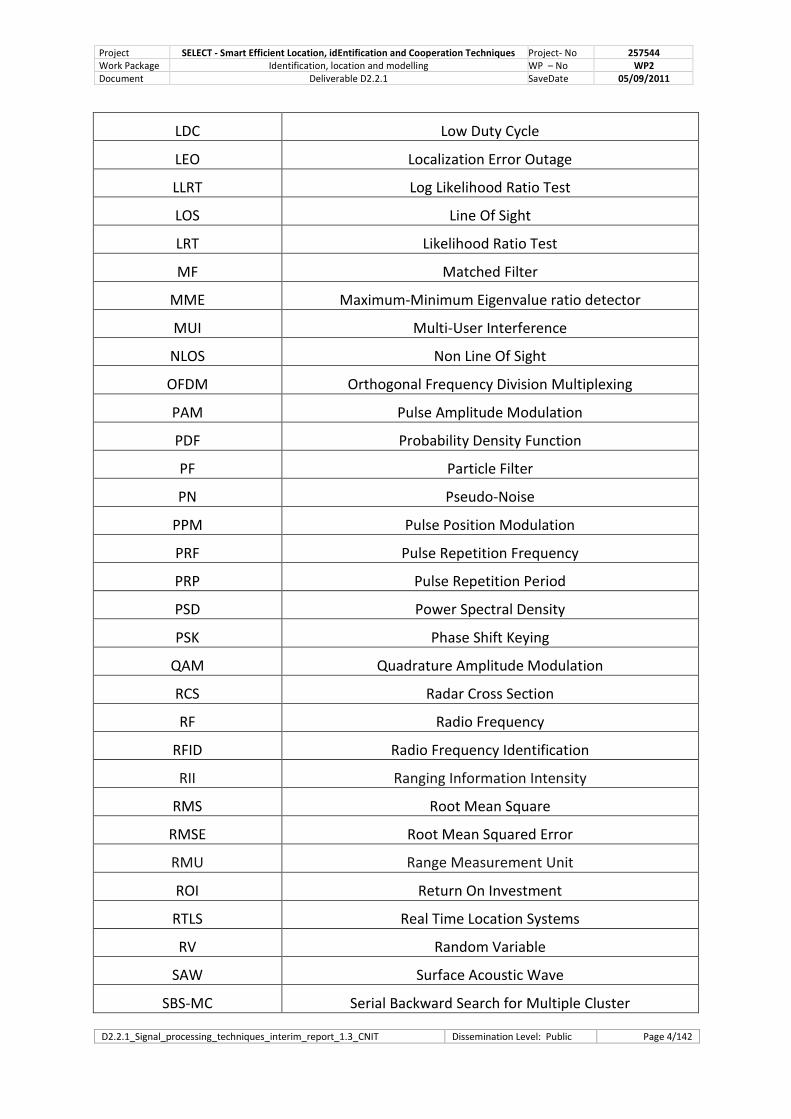
LDC Low Duty Cycle
LEO Localization Error Outage
LLRT Log Likelihood Ratio Test
LOS Line Of Sight
LRT Likelihood Ratio Test
MF Matched Filter
MME Maximum-Minimum Eigenvalue ratio detector
MUI Multi-User Interference
NLOS Non Line Of Sight
OFDM Orthogonal Frequency Division Multiplexing
PAM Pulse Amplitude Modulation
PDF Probability Density Function
PF Particle Filter
PN Pseudo-Noise
PPM Pulse Position Modulation
PRF Pulse Repetition Frequency
PRP Pulse Repetition Period
PSD Power Spectral Density
PSK Phase Shift Keying
QAM Quadrature Amplitude Modulation
RCS Radar Cross Section
RF Radio Frequency
RFID Radio Frequency Identification
RII Ranging Information Intensity
RMS Root Mean Square
RMSE Root Mean Squared Error
RMU Range Measurement Unit
ROI Return On Investment
RTLS Real Time Location Systems
RV Random Variable
SAW Surface Acoustic Wave
SBS-MC Serial Backward Search for Multiple Cluster
Project SELECT - Smart Efficient Location, idEntification and Cooperation Techniques Project- No 257544 Work Package Identification, location and modelling WP – No WP2 Document Deliverable D2.2.1 SaveDate 05/09/2011
D2.2.1_Signal_processing_techniques_interim_report_1.3_CNIT Dissemination Level: Public Page 5/142
SCM Supply Chain Management
SCR Signal-to-Clutter Ratio
SIR Signal-to-Interference Ratio
SIS Sequential Importance Sampling
SNR Signal-to-Noise Ratio
SOA State Of Art
SPEB Squared Position Error Bound
SPMF Single-Path Matched Filter
SQNR Signal-to-Quantization-Noise-Ratio
TDM Time Division Multiplexing
TDOA Time Difference Of Arrival
TOA Time-of-Arrival
UHF Ultra-High Frequency
UWB Ultra-Wideband Technology
VNA Vector Network Analyzer
WSN Wireless Sensor Network
WSR Wireless Sensor Radar
Project SELECT - Smart Efficient Location, idEntification and Cooperation Techniques Project- No 257544 Work Package Identification, location and modelling WP – No WP2 Document Deliverable D2.2.1 SaveDate 05/09/2011
D2.2.1_Signal_processing_techniques_interim_report_1.3_CNIT Dissemination Level: Public Page 6/142
EXECUTIVE SUMMARY
The signal processing techniques interim report D2.2.1 presents results of the activity carried out in tasks T2.2, T2.3 and T2.4 related to, respectively, “Passive communication schemes based on signal backscattering”, “High-accuracy active and passive location and tracking algorithms” and “Coexistence and interference mitigation techniques”. It provides the preliminary system architecture design guidelines, analysis, and results.
First, the analysis of potential candidate technologies able to fit the SELECT project requirements is presented.
Different aspects related to signal format definition, tag and reader signal processing schemes are addressed with the purpose to achieve reliable tag-reader communication and tag tracking accuracy. Through the report, the constraints on system design derived from application requirements (work package WP1), propagation effects (task 2.1), spectrum usage regulatory limitations (task 2.4) and technological issues (work packages WP3/WP4) are accounted for.
The last part of the document discusses the main critical issues and next activity directions.
This report provides the inputs for system architecture design (task T2.5), tag design (work package WP3) and reader design (work package WP4).
Project SELECT - Smart Efficient Location, idEntification and Cooperation Techniques Project- No 257544 Work Package Identification, location and modelling WP – No WP2 Document Deliverable D2.2.1 SaveDate 05/09/2011
D2.2.1_Signal_processing_techniques_interim_report_1.3_CNIT Dissemination Level: Public Page 7/142
INTRODUCTION: THE SELECT PROJECT
The SELECT project focuses on studying innovative solutions enabling high-accuracy detection, identification, and location of objects/persons equipped with small ultra-low power tags using a network of intelligent self-configuring radio devices. Network functionalities will be enhanced to include the detection and tracking of moving objects/persons without tags eventually present in the same area.
To achieve this goal, several technologies such as radio frequency identification (RFID), ultra wideband backscattering modulation, time reversal, relaying, and associated advanced algorithms, will be considered and partly or totally integrated in a demonstrator. This will require the design of multi-frequency/multi-technology tags for system-neutral identification along the use lifetime of a tag, based on advanced concepts in low-consumption chip and antenna design.
Innovative techniques will be considered to improve the location accuracy, increase tag energy efficiency and extend system coverage by a mixture of progress in the system architecture, in the detection and tag activation techniques, and in the complexity-performance trade off of chip design.
Special emphasis will be given to the analysis and design of “green” solutions by considering low complexity and low power tags through the exploitation of passive communication (without integrated tag batteries) as well smart cooperation strategies.
Finally, single system components and the overall system performance will be validated through experimental characterization, hardware implementation, as well as simulation.
Identification/detection reliability, tracking accuracy, power consumption will be amongst the major evaluation criteria.
A wireless network integrating detection, identification, and location would lead to relevant improvements in the development of a wide range of advanced applications including logistics (package tracking) and supply chain management (SCM)
Project SELECT - Smart Efficient Location, idEntification and Cooperation Techniques Project- No 257544 Work Package Identification, location and modelling WP – No WP2 Document Deliverable D2.2.1 SaveDate 05/09/2011
D2.2.1_Signal_processing_techniques_interim_report_1.3_CNIT Dissemination Level: Public Page 8/142
Table of contents LIST OF ACRONYMS .......................................................................................................................................... 3
NEXT STEPS .............................................................................................................................................. 137
LITERATURE ................................................................................................................................................. 139
Project SELECT - Smart Efficient Location, idEntification and Cooperation Techniques Project- No 257544 Work Package Identification, location and modelling WP – No WP2 Document Deliverable D2.2.1 SaveDate 05/09/2011
D2.2.1_Signal_processing_techniques_interim_report_1.3_CNIT Dissemination Level: Public Page 11/142
Project SELECT - Smart Efficient Location, idEntification and Cooperation Techniques Project- No 257544 Work Package Identification, location and modelling WP – No WP2 Document Deliverable D2.2.1 SaveDate 05/09/2011
D2.2.1_Signal_processing_techniques_interim_report_1.3_CNIT Dissemination Level: Public Page 12/142
CONTENT
One of the main objectives of the SELECT project is the investigation and evaluation of new architectures based on a combination of readers and relays to significantly extend the operational detection range of the tags with high-accuracy tracking capabilities, while optimizing the complexity, energy efficiency, and cost. The easy integration with current UHF Gen2 tags is also an important aspect undertaken [6].
The requirements of a configurable SELECT system concept for identification, detection and location have been defined in work package WP1 [3], [2]. They pose several scientific and technological challenges which, in part, are analyzed in this report. For what the communication and tracking capabilities are regarded, the “centre of gravity” technology of the SELECT project is ultra-wide bandwidth (UWB). Its adoption leads to some advantages in terms of ranging/positioning accuracy, multi-tag capability, and interference rejection.
In this interim report, existing or under study UWB technologies and solutions for tag-reader communication and tracking are analyzed and compared in section 1 with reference to the requirements of the SELECT project [3], [2]. To reduce the complexity and energy consumption, the adoption of active devices is avoided in favor of semi-passive tags based on backscatter communication. They are characterized by extremely low energy consumption and hence they are capable of working for years with small green batteries or in conjunction with energy harvesting techniques [5].
Communication between tags and readers using backscatter signaling is addressed in section 2 through the definition of the tag/reader architecture as well as the signaling format. A discussion on parameters design criteria is provided and supported by some preliminary numerical results in section 3.
Section 4 addresses the issue of synchronization and ranging through the estimation of the time-of-arrival (TOA) of the response signal backscattered by the tag. Algorithms and results for localization and tracking in the SELECT reference scenario are reported in section 5. Finally coexistence and interference issues are treated in section 6 where preliminary analysis on spectrum sensing techniques and LDC constraints are presented.
Project SELECT - Smart Efficient Location, idEntification and Cooperation Techniques Project- No 257544 Work Package Identification, location and modelling WP – No WP2 Document Deliverable D2.2.1 SaveDate 05/09/2011
D2.2.1_Signal_processing_techniques_interim_report_1.3_CNIT Dissemination Level: Public Page 13/142
1. Candidate Backscattering Communication Techniques
This section presents a state of the art survey of low-cost, low-energy consumption UWB tags of potential interest for the SELECT project.
Several UWB Real Time Locating System solutions already exist. They are supported by IEEE standards: namely IEEE 802.15.4a or IEEE 802.15.4f. For the moment, the proprietary solutions (Timedomain, Ubisense, Decawave, ZES, etc…) based on these standards are all designed for active tags.
Contrarily, passive or semi-passive RFID are particularly attractive due to their low cost. Different passive or semi-passive tags technologies are being developed:
Backscatter modulation
Active modulation (tag radio-powered)
Chipless passive tags
Regarding these kind of passive schemes, the problem lies in the powering of the tag. Indeed, it is not possible to extract energy from UWB signals. The UWB FCC/EU power emission mask constrains the transmitted power to be less than 1mW (vs. 2-4W for UHF RFID). This available RF power is not sufficient to energize the tag at distances of interest (>1m).
At the tag level, the energy can thus be obtained either from a small battery, from a UHF signal, or from energy harvesting, which increases the tag dimension and complexity.
The investigation of energy harvesting techniques is beyond the scope of the SELECT project, however the design of extremely low consumption tag would enable in the near future the adoption of such techniques. Then, within the SELECT project, energy efficient tag solutions for communication and accurate ranging will be investigated.
In this section, the three main passive or semi-passive tags technologies are described.
1.1 Backscatter Modulation
The main principles of backscatter communication using UWB signals are recalled here after, as well as alternative comparative solutions.
1.1.1 Backscatter modulation basics and SOA solutions
The main principle of a backscattering communication scheme presented in [8] is illustrated in Figure 1-1. The reader transmits an UWB pulse which is backscatter by the tag.
The problem is that the reflected signals coming from surrounding objects (clutter) and antenna structural mode are in general dominant (green pulses).
This effect emphasizes the need for an efficient signal structure design and an appropriate signal processing to mitigate the effect of clutter as will be addressed in section 2.
Project SELECT - Smart Efficient Location, idEntification and Cooperation Techniques Project- No 257544 Work Package Identification, location and modelling WP – No WP2 Document Deliverable D2.2.1 SaveDate 05/09/2011
D2.2.1_Signal_processing_techniques_interim_report_1.3_CNIT Dissemination Level: Public Page 14/142
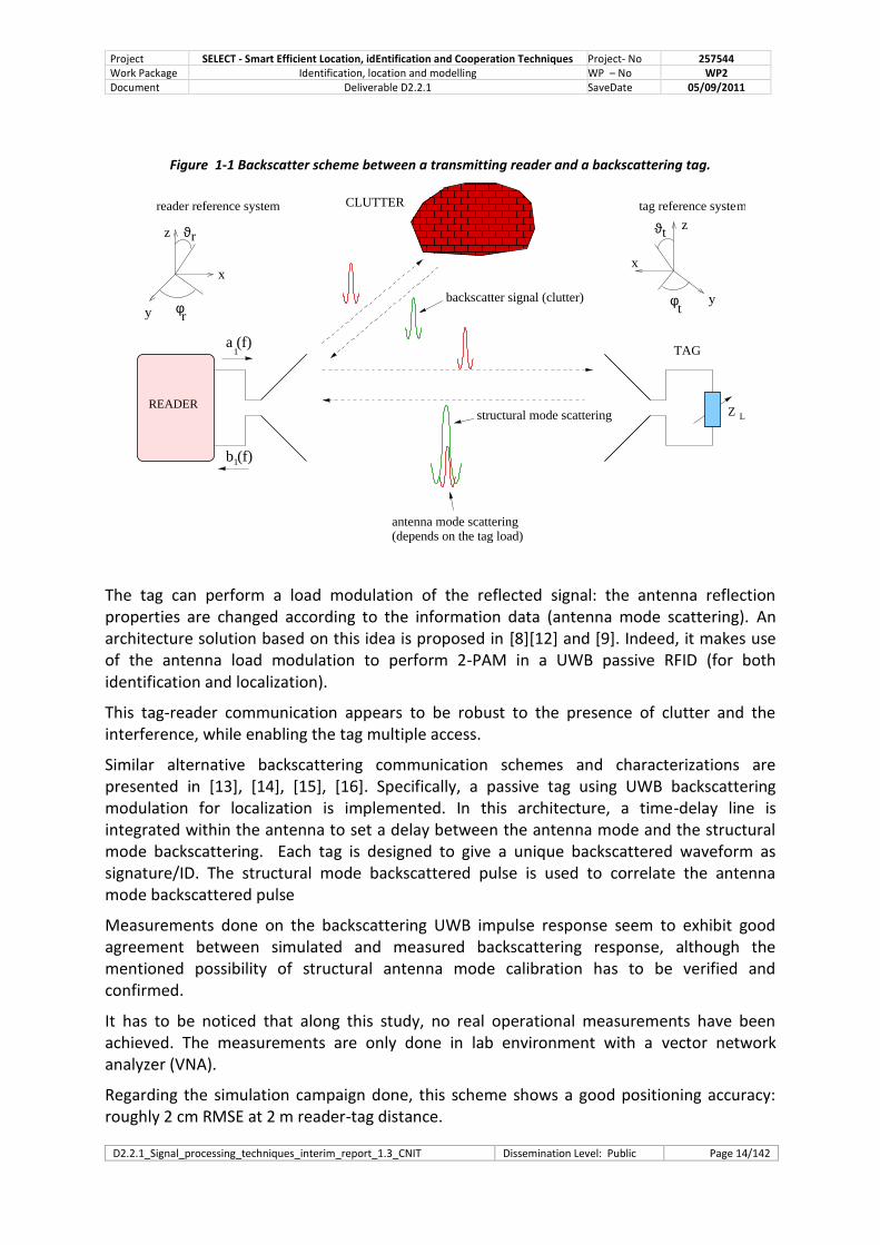
Figure 1-1 Backscatter scheme between a transmitting reader and a backscattering tag.
(depends on the tag load)
y
zz
y
x
rf
t
Jtr
Z L
READER
1
backscatter signal (clutter)
TAG
CLUTTER
a (f)
b (f)
1
tag reference systemreader reference system
f
J
structural mode scattering
antenna mode scattering
x
The tag can perform a load modulation of the reflected signal: the antenna reflection properties are changed according to the information data (antenna mode scattering). An architecture solution based on this idea is proposed in [8][12] and [9]. Indeed, it makes use of the antenna load modulation to perform 2-PAM in a UWB passive RFID (for both identification and localization).
This tag-reader communication appears to be robust to the presence of clutter and the interference, while enabling the tag multiple access.
Similar alternative backscattering communication schemes and characterizations are presented in [13], [14], [15], [16]. Specifically, a passive tag using UWB backscattering modulation for localization is implemented. In this architecture, a time-delay line is integrated within the antenna to set a delay between the antenna mode and the structural mode backscattering. Each tag is designed to give a unique backscattered waveform as signature/ID. The structural mode backscattered pulse is used to correlate the antenna mode backscattered pulse
Measurements done on the backscattering UWB impulse response seem to exhibit good agreement between simulated and measured backscattering response, although the mentioned possibility of structural antenna mode calibration has to be verified and confirmed.
It has to be noticed that along this study, no real operational measurements have been achieved. The measurements are only done in lab environment with a vector network analyzer (VNA).
Regarding the simulation campaign done, this scheme shows a good positioning accuracy: roughly 2 cm RMSE at 2 m reader-tag distance.
Project SELECT - Smart Efficient Location, idEntification and Cooperation Techniques Project- No 257544 Work Package Identification, location and modelling WP – No WP2 Document Deliverable D2.2.1 SaveDate 05/09/2011
D2.2.1_Signal_processing_techniques_interim_report_1.3_CNIT Dissemination Level: Public Page 15/142
Additionally, the results show that it is feasible to identify the passive tag employing pulse-polarity and pulse-position. Moreover, this study establishes the relative easiness to get the characteristics time delay between antenna and structural mode backscattering pulses.
For Ep/N0 = 30dB, it has been demonstrated that 20 tags can be supported with a probability of detection error less than 1%. This represents a low number of tags supported far from the SELECT project requirements.
It has to be noticed that this study does not account for a proof of concept.
Another backscattering communication architecture is presented in [17]. This solution differs from the previous one with the fact that it implements a UHF signal for tag power supply and communication, and a backscattering modulation UWB for ranging. The principle of this architecture is illustrated in Figure 1-2. It is also made use here of tag load modulation. Contrarily to the previous study, this one represents a proof of concept. Nevertheless, the ranging accuracy has not been studied.
Figure 1-2 Backscattering communication pulse implementing an UHF powering signal [17].
1.1.2 Conclusion
As a conclusion, the pro and cons of the passive backscattering communication scheme can be listed.
This technology presents the following advantages:
It is a simple technology
The complexity is concentrated mainly at the reader side
It is easily integrable with UHF tags
It exhibits low energy consumption (energy needed only for the micro-controller and not for the RF stage)
Semi-passive tag
In the framework of the SELECT project, the patent license is held by the SELECT consortium
The disadvantages of this technology are summarized here after:
Project SELECT - Smart Efficient Location, idEntification and Cooperation Techniques Project- No 257544 Work Package Identification, location and modelling WP – No WP2 Document Deliverable D2.2.1 SaveDate 05/09/2011
D2.2.1_Signal_processing_techniques_interim_report_1.3_CNIT Dissemination Level: Public Page 16/142
Code synchronization is an issue between reader and tag (design of synchronization schemes at the reader needed, problem reduced if used in conjunction with UHF technology), using for example wake-up synchronization signals.
The link budget penalty with respect to active UWB modulation tags might limit the operating range.
1.2 Chipless Tags
This section concerns the chipless fully passive tag. Backscattering solution minimizing tag cost and/or size are presented.
1.2.1 Inkjet printable fully passive RFID tag
This solution is presented in[20], where a very simple circuit is printed with a metallic ink on a support. 8-bit data are encoded by impedance mismatch along the transmission line printed on the material. Planar capacitors are pre-printed, and connected via intersection printed to the transmission line.
Figure 1-3 RFID tag using inkjet printing.
The main advantages of this technique are listed below:
Fully passive tag
Very low cost Inkjet Printing Technology can be used
No synchronization problems for the reader-tag codes
The disadvantages are summarized here after:
Link budget to be studied, no results found (it expected to be worse than other technologies, long transmission lines attenuation)
Dimensions problem: in an 8-bit code takes 40cm transmission line length using a 0.4ns Gaussian pulse as incoming signal
“Disposable” tags (not reconfigurable)
81 ID tags maximum (with 8 bits): not enough
Project SELECT - Smart Efficient Location, idEntification and Cooperation Techniques Project- No 257544 Work Package Identification, location and modelling WP – No WP2 Document Deliverable D2.2.1 SaveDate 05/09/2011
D2.2.1_Signal_processing_techniques_interim_report_1.3_CNIT Dissemination Level: Public Page 17/142
Tag-collision issues in a multi access context: 8 bits code too short, high cross-correlation.
Time division multiplexing (TDM) with acknowledgement not possible
40 cm transmission line on a specific inkjet printed circuit: high insertion loss? (no data available)
1.2.2 Multiresonator
The chipless tag encodes data into the spectral domain in both magnitude and phase of the spectrum [24]. The RFID reader frequency range is between 5GHz and 10.7GHz. It successfully detects a chipless tag at 15cm range.
Figure 1-4 Photo of the UWB 35-bit chipless RFID tag.
It can be seen on Figure 1-4 an example of spectral signature obtained with the multiresonator.
Figure 1-5 Measured attenuation of 23-bit multiresonator.
The main advantages of this technique are listed below:
Project SELECT - Smart Efficient Location, idEntification and Cooperation Techniques Project- No 257544 Work Package Identification, location and modelling WP – No WP2 Document Deliverable D2.2.1 SaveDate 05/09/2011
D2.2.1_Signal_processing_techniques_interim_report_1.3_CNIT Dissemination Level: Public Page 18/142
Fully passive tag
Fully printable
No synchronization problems for the reader-tag codes
The disadvantages are summarized here after:
Link budget to be studied, no results found (it expected to be worse than other technologies, long transmission lines attenuation)
Dimensions (delay lines length). Probably smaller with respect to solution 1.2.1
A 9x7cm tag is capable of 35bit coding
“Disposable” tags (not reconfigurable)
Doubts about its ability to work in the presence of multipath (no studies found)
Interrogation of the tag by sweeping the RF signal frequency: it is not IR-UWB: could yield to higher interferences and/or not respect of the 15.4a regulation mask
Detection based on the spectrum signature: high sensitivity to interference, poor ranging accuracy
Reader and tag antennas must be cross-polarized: significant restrictions in tag positioning and orientation
Ranging with the signal phase is ambiguous
Identification efficiency but high ranging error: phase estimation error up to 42°
Not more than 15 cm range
1.2.3 SAW devices
This technique makes use of orthogonal frequency coding associated with a SAW based tag. This tag consists of an input transducer that launches a surface wave on a substrate towards an array of single frequency collinear reflectors that reflect the wave back to the input after providing ID coding within the reflections[21].
Figure 1-6 SAW tag example.
The main advantages of this technique are listed below:
Project SELECT - Smart Efficient Location, idEntification and Cooperation Techniques Project- No 257544 Work Package Identification, location and modelling WP – No WP2 Document Deliverable D2.2.1 SaveDate 05/09/2011
D2.2.1_Signal_processing_techniques_interim_report_1.3_CNIT Dissemination Level: Public Page 19/142
Fully passive tag
Very small dimension and attenuation. [22][23] show the possibility of a 1x1mm tag with 3dB of insertion loss
No synchronization problems for the reader-tag codes
PN-OFC-TDM technique: allows a greater number of users operating in the same frequency band without increasing the frequency
The disadvantages are summarized here after:
Reading distance below 3-5 meters for [22] (2 feet range success for [21]) =>this range is clearly too low for SELECT applications
Acoustic technology (cost?)
“Disposable” tags (not reconfigurable)
Autocorrelation function with large central peak (28 ns): poor ranging precision achievable
Cannot be used on every material, not working on plastic for example (due to piezoelectric nature)
Operational frequency impact? (tested one is 250MHz)
High loss and poor temporal resolution
1.3 Active Modulation
All the backscattering solutions presented in this section implement additionally to the UWB signal, a narrow band UHF signal. Very similar solutions are developed in [17], [25], [26], [27], [28].
In general, a narrowband downlink (tag interrogation command, tag powering) is used. Tags capture its power by power scavenging. The UWB uplink signal with an active pulse transmitter is used for localization purpose.
Figure 1-7 Radio-powered module with asymmetric link using UWB for RFID [25].
Project SELECT - Smart Efficient Location, idEntification and Cooperation Techniques Project- No 257544 Work Package Identification, location and modelling WP – No WP2 Document Deliverable D2.2.1 SaveDate 05/09/2011
D2.2.1_Signal_processing_techniques_interim_report_1.3_CNIT Dissemination Level: Public Page 20/142
Figure 1-8 RF tag and reader with asymmetric communication bandwidth-solution proposed in [26].
Figure 1-9 RFID based on ultra-wideband time-hopped pulse-position modulation – solution proponed in [27].
The main advantages of these techniques are listed below:
Less path loss constraints (active UWB modulation on the tag side)
Simpler code synchronization respect to the UWB backscattering solution
Easily integrable with UHF Tags
Asymmetric UHF for downlink, IR-UWB for uplink: => reduce the complexity of the tag
TDM with acknowledgement protocol: decreases the tag-collision
High network throughput: 2000 tag per second for example in [25]
Good operational range: 10m range [25]
The disadvantages are summarized here after:
Project SELECT - Smart Efficient Location, idEntification and Cooperation Techniques Project- No 257544 Work Package Identification, location and modelling WP – No WP2 Document Deliverable D2.2.1 SaveDate 05/09/2011
D2.2.1_Signal_processing_techniques_interim_report_1.3_CNIT Dissemination Level: Public Page 21/142
Tag complexity and costs (complete UWB transmitter or transceiver needed at the tag side)
Tag power consumption (no energy harvesting techniques can be used to power up the UWB tag)
Asymmetric link make the ranging more complex, and could decrease the ranging accuracy (clock impairment between tag and reader?)
TDM with acknowledgement protocol: increases the complexity of ranging procedure
System efficiency decrease rapidly when the difference between frame size and number of tag increase. Could yield problem with a high number of tag scenario
It has to be noticed that these techniques are only a conjunction of available technologies, and do not represent a major innovation. Moreover several patents are pending on these solutions.
1.4 Comparison and Conclusion
As a conclusion, the table below summarizes all the SOA backscattering techniques available described here and establishes the main points of comparison.
Table 1-1 Comparison of the different SOA backscattering techniques.
backscatter
modulation
chipless tag :
impedance
mismatch
chipless tag :
multiresonator
chipless tag : SAW
technology
active
modulation tag
basic concept
Use of the antenna load
modulation to perform
UWB passive RFID (for
both identification and
localization)
8 bit inkjet printable
fully passive RFID tag
tag encoding data into
the spectral signature
in both magnitude and
phase
UWB orthogonal
frequency and TDM
protocel coding for a
SAW chipless tag
radio-powered
module with
asymmetric link using
UWB for RFID
strong limitations- link budget penalty
- backscattering antenna
mode issue
- dimension of the
circuit
- link budget
- link budget
- short range
- poor ranging
accuracy expected
- link budget
- short range
- poor ranging accuracy
expected
- tag complexity and
cost
- tag power
consumption
- clocks synchro?
preliminary
opinion on
SELECT project
requirements
meeting
+ + - - - + +
From the above reported analysis it can be concluded that (semi)-passive tags based on UWB backscatter modulation represent a good trade-off between performance, complexity and energy efficiency. In particular the adoption of the UWB backscatter modulation technology offers:
Good design flexibility as both stand-alone UWB tag or hybrid UWB/UHF Gen2 tag architectures are possible.
Good potential ranging capabilities, thus enabling high-accuracy location and tracking.
Project SELECT - Smart Efficient Location, idEntification and Cooperation Techniques Project- No 257544 Work Package Identification, location and modelling WP – No WP2 Document Deliverable D2.2.1 SaveDate 05/09/2011
D2.2.1_Signal_processing_techniques_interim_report_1.3_CNIT Dissemination Level: Public Page 22/142
Low energy required to power up the tag, thus allowing the adoption of small, even green, batteries or energy harvesting techniques.
Low cost.
Project SELECT - Smart Efficient Location, idEntification and Cooperation Techniques Project- No 257544 Work Package Identification, location and modelling WP – No WP2 Document Deliverable D2.2.1 SaveDate 05/09/2011
D2.2.1_Signal_processing_techniques_interim_report_1.3_CNIT Dissemination Level: Public Page 23/142
2 Definition of Reader and Tag Architectures
The aim of this section is to describe the reader and tag architectures as well as signals format capable of enabling reliable communication through backscatter modulation. The following paragraphs present in details the functional blocks of the reader and tag, signal format, and the mathematical description of signal processing in the different parts of the system.
The basic principle of the UWB backscatter modulation has been described in section 1.1 and can be found in [12][11][10][14].
2.1 Reader Architecture
Figure 1-10 proposes the architecture scheme for the reader, which is composed of a transmitter and a receiver section. In the following paragraph we focus on the transmitter section, while the receiving part is object of paragraph 3 where signal-processing schemes for data demodulation are illustrated.
2.1.1 Functional blocks – Transmitter Section
With reference to the scheme reported in Figure 1-10, the transmitter section is composed of a UWB pulse generator with pulse template p(t) and of a spreading sequence (reader’s code) generator that produces an antipodal binary sequence {d
n} of length N
c symbols
(chips). Each chip modulates in amplitude the transmitted pulses (PAM modulator) as will be illustrated in more details later. The generated signal is sent to the antenna connector and radiated in air.
Figure 1-10 Reader functional blocks.
TOA tag code
ReceiverEstimator
TOA
Ns
decodedbits
d
d
c
n
n
n
v(t)
Transmitter
reader code pulse
generatorseq. generator
Matched
filterDetector
ym
TX antenna
RX antenna
UWB READER
ADC
tag code
seq. generator acquisition
Project SELECT - Smart Efficient Location, idEntification and Cooperation Techniques Project- No 257544 Work Package Identification, location and modelling WP – No WP2 Document Deliverable D2.2.1 SaveDate 05/09/2011
D2.2.1_Signal_processing_techniques_interim_report_1.3_CNIT Dissemination Level: Public Page 24/142
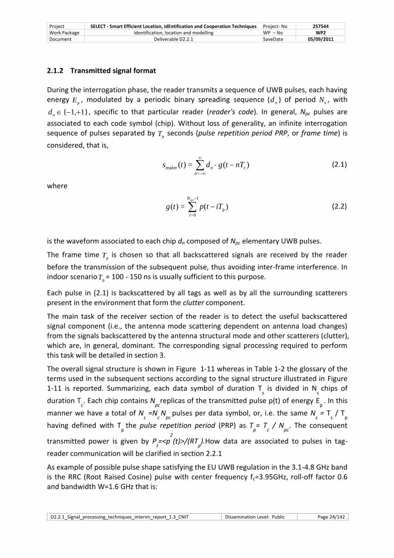
2.1.2 Transmitted signal format
During the interrogation phase, the reader transmits a sequence of UWB pulses, each having energy
pE , modulated by a periodic binary spreading sequence }{ nd of period sN , with
1}1,{ nd , specific to that particular reader (reader's code). In general, Npc pulses are
associated to each code symbol (chip). Without loss of generality, an infinite interrogation sequence of pulses separated by
pT seconds (pulse repetition period PRP, or frame time) is
considered, that is,
)(=)( c
=
reader nTtgdts n
n
where
)(=)( p
1
0=
iTtptgpcN
i
is the waveform associated to each chip dn composed of Npc elementary UWB pulses.
The frame time pT is chosen so that all backscattered signals are received by the reader
before the transmission of the subsequent pulse, thus avoiding inter-frame interference. In indoor scenario
pT = 100 - 150 ns is usually sufficient to this purpose.
Each pulse in (2.1) is backscattered by all tags as well as by all the surrounding scatterers present in the environment that form the clutter component.
The main task of the receiver section of the reader is to detect the useful backscattered signal component (i.e., the antenna mode scattering dependent on antenna load changes) from the signals backscattered by the antenna structural mode and other scatterers (clutter), which are, in general, dominant. The corresponding signal processing required to perform this task will be detailed in section 3.
The overall signal structure is shown in Figure 1-11 whereas in Table 1-2 the glossary of the terms used in the subsequent sections according to the signal structure illustrated in Figure 1-11 is reported. Summarizing, each data symbol of duration T
s is divided in N
c chips of
duration Tc. Each chip contains N
pcreplicas of the transmitted pulse p(t) of energy E
p . In this
manner we have a total of Ns =N
c N
pc pulses per data symbol, or, i.e. the same N
s = T
s / T
p
having defined with Tp
the pulse repetition period (PRP) as Tp= T
c / N
pc. The consequent
transmitted power is given by Pt=<p
2
(t)>/(RTp).How data are associated to pulses in tag-
reader communication will be clarified in section 2.2.1
As example of possible pulse shape satisfying the EU UWB regulation in the 3.1-4.8 GHz band is the RRC (Root Raised Cosine) pulse with center frequency fc=3.95GHz, roll-off factor 0.6 and bandwidth W=1.6 GHz that is:
(2.1)
(2.2)
Project SELECT - Smart Efficient Location, idEntification and Cooperation Techniques Project- No 257544 Work Package Identification, location and modelling WP – No WP2 Document Deliverable D2.2.1 SaveDate 05/09/2011
D2.2.1_Signal_processing_techniques_interim_report_1.3_CNIT Dissemination Level: Public Page 25/142
(2.3)
)2cos(/41
1/)1(sin
/4
1/)1(cos
4)(
2tf
tttt
tttt
ttp c
p
p
p
p
p
where β is the roll-off factor, fc the center frequency, and tp a parameter such that
.
Figure 1-11 Data packet structure. s
N2 r1
1 2 N c
d0 d1 dN −1c
1 2 N pc
time
T p
Tc
T
Project SELECT - Smart Efficient Location, idEntification and Cooperation Techniques Project- No 257544 Work Package Identification, location and modelling WP – No WP2 Document Deliverable D2.2.1 SaveDate 05/09/2011
D2.2.1_Signal_processing_techniques_interim_report_1.3_CNIT Dissemination Level: Public Page 26/142
Table 1-2 Symbols Definition.
Symbol Description
{dn} reader’s spreading code of length N
c1}1,{ nd
{cn} tag’s spreading code of length N
c1}1,{ nd
{bn} tag’s data sequence 1}1,{ nd
Nc number of chips per data symbol (must be the same in the tag)
Npc
number of pulses emitted per chip
Ns =N
c N
pc number of pulses emitted per symbol
Nr number of bits per interrogation packet
Tp pulse repetition period (PRP) or frame time
Rp=1/T
p pulse repetition frequency (PRF)
Tc=T
pN
pc chip time
Rc=1/T
c chip rate (must be the same in the tag)
Ts= T
c N
c symbol (bit) time
Rb=1/T
s symbol rate (data rate) (must be the same in the tag)
Pt=E
p/T
p transmitted power (Watt)
Ep=<p
2
(t)>/R pulse energy (J)
R antenna impedance (Ohm)
p(t) transmitted pulse shape (V)
2.2 Tag Architecture
In order to make the reader able to distinguish between different tags and detect the useful signal immersed in the clutter a modulation scheme has to be adopted by the tag as will be presented in this section. A quite general backscatter modulator architecture is presented in Figure 1-12 which allows for different signaling schemes such as PAM (Pulse Amplitude Modulation), PPM (Pulse Position Modulation) and ON-OFF keying.
Project SELECT - Smart Efficient Location, idEntification and Cooperation Techniques Project- No 257544 Work Package Identification, location and modelling WP – No WP2 Document Deliverable D2.2.1 SaveDate 05/09/2011
D2.2.1_Signal_processing_techniques_interim_report_1.3_CNIT Dissemination Level: Public Page 27/142
Figure 1-12 Backscatter modulator architecture.
However, the general structure of Figure 1-12 requires costly and space consuming UWB delay lines leading to a tag not satisfying the SELECT requirements. Then a simplified tag architecture version that considers 2-PAM signaling is analyzed. In this case, the backscatter modulator reduces to a simple switch (switch S1 as in figure).
2.2.1 Tag Functional blocks
Figure 1-13 shows the functional blocks that compose the tag. The device is connected to a wideband UHF/UWB antenna (or also two separated antennas) and two different sections (UHF and UWB) are responsible for signal processing and power management of the narrowband and wideband signal components, respectively. More in particular the UHF part is composed of a standard Gen2 UHF RFID driven by appropriate control logic. Since a standard UHF tag is already composed of a power management unit that extract energy from the interrogation UHF signal, the same unit could be used to detect an eventual wake up signal to switch the UWB section on and provide a synchronization signal [6].
The UWB section is powered by a battery (semi-passive tag) and composed of a simple control logic that generates the data bits to be transmitted (for example the tag ID) and the spreading code necessary to allow multiple access and clutter removal as will be explained in the following sections. The RF stage consists of a simple UWB switch driven by the composite sequence given by the modulo-2 product between the data bit and the spreading code.
Project SELECT - Smart Efficient Location, idEntification and Cooperation Techniques Project- No 257544 Work Package Identification, location and modelling WP – No WP2 Document Deliverable D2.2.1 SaveDate 05/09/2011
D2.2.1_Signal_processing_techniques_interim_report_1.3_CNIT Dissemination Level: Public Page 28/142
Figure 1-13 Tag functional blocks.
{c }
UHF/UWB antenna
RFID modem
Power
management
control
batterycontrol logic
data (ID)
memory
spread code
memory
switch
m(t)XOR
n
f
f
data
chip
mem
ory
wake−up
UWB TAG
STANDARD UHF TAG
logic
Consider now a scenario where a reader interrogates tagN tags located in the same area. To
make the uplink communication between the k -th tag and the reader robust to the presence of clutter, interference, and to allow multiple access, each tag is designed to change its status (short or open circuit) at each chip time
cT according to the data to be
transmitted and a periodic tag's code }{ )(k
nc , with 1}1,{)( k
nc , of period sN . Specifically,
each tag information symbol 1}1,{)( k
nb is associated to sN pulses, thus the symbol
duration equals sps = NTT . In this way the polarity of the reflected signal changes according
to the tag's code sequence during a symbol time, whereas the information symbol affects the entire sequence pulse's polarity at each symbol.
The reader and the tags have their own independent clock sources and hence they have to
be treated as asynchronous. Let us denote )(
f
)()( = kkk uT , with )(ku integer and
f
)( <0 Tk , the clock offset of the k -th tag with respect to the reader's clock. In case a
wake-up signal is available, then reader and tags spreading codes can be considered aligned
(synchronous) and hence 0)( ku , whereas )(k in general may be different from zero due to
the unknown propagation delays.
Therefore, the backscatter modulator signal, commanding the tag's switch, can be expressed as
)(
cs
c
)()(
1s
0=
1
0=
)( 1=)( kk
n
k
i
N
i
N
n
k iTnTtT
bctmr
Project SELECT - Smart Efficient Location, idEntification and Cooperation Techniques Project- No 257544 Work Package Identification, location and modelling WP – No WP2 Document Deliverable D2.2.1 SaveDate 05/09/2011
D2.2.1_Signal_processing_techniques_interim_report_1.3_CNIT Dissemination Level: Public Page 29/142
)(
c
)(
c
)()(1
0=
)(1
= kkk
nf
k
n
N
n
TuntT
bcr
having defined s/Nnnf and 1)( t for [0,1]t and zero otherwise.1
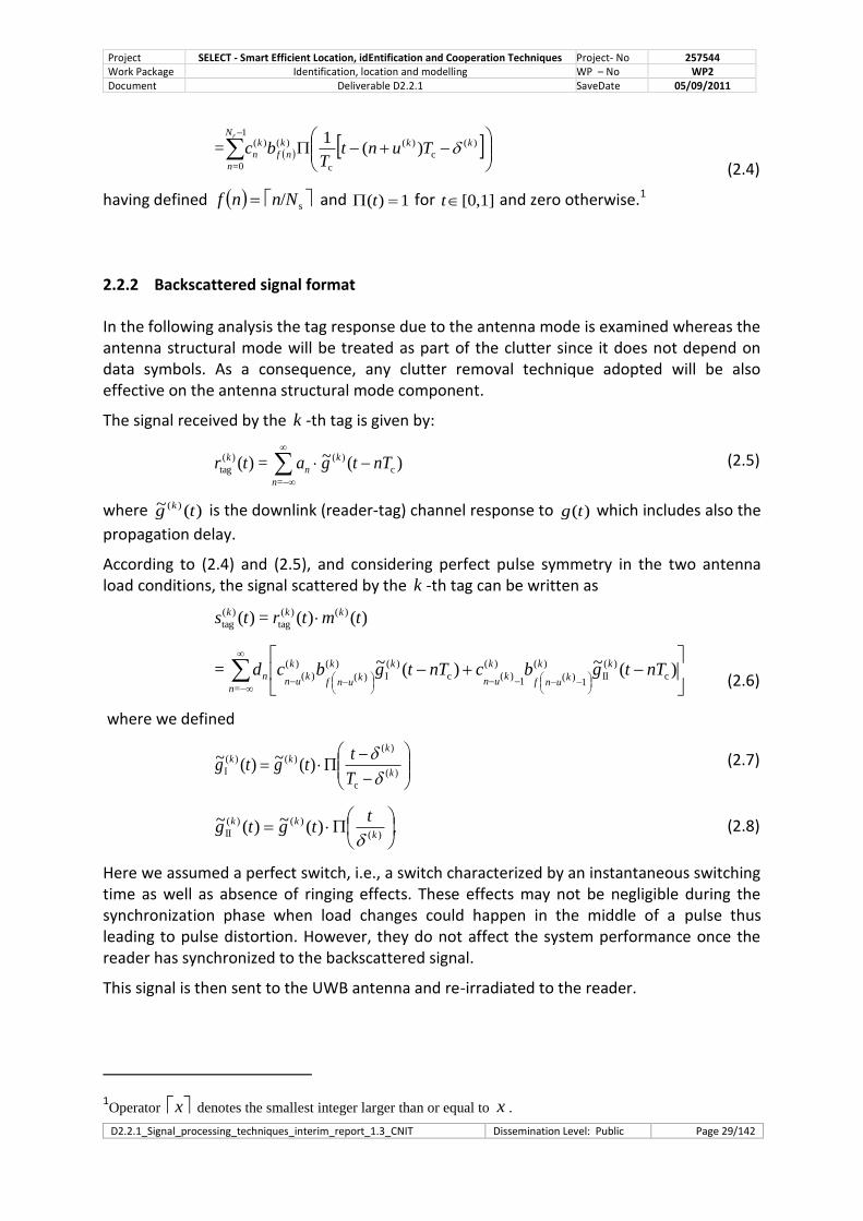
2.2.2 Backscattered signal format
In the following analysis the tag response due to the antenna mode is examined whereas the antenna structural mode will be treated as part of the clutter since it does not depend on data symbols. As a consequence, any clutter removal technique adopted will be also effective on the antenna structural mode component.
The signal received by the k -th tag is given by:
)(~=)( c
)(
=
)(
tag nTtgatr k
n
n
k
where )(~ )( tg k is the downlink (reader-tag) channel response to )(tg which includes also the
propagation delay.
According to (2.4) and (2.5), and considering perfect pulse symmetry in the two antenna load conditions, the signal scattered by the k -th tag can be written as
)()(=)( )()(
tag
)(
tag tmtrts kkk
)(~)(~= c
)(
II
)(
1)(
)(
1)(c
)(
I
)(
)(
)(
)(
=
nTtgbcnTtgbcd kk
kunf
k
kun
kk
kunf
k
kun
n
n
where we defined
)(
c
)()()(
I )(~)(~k
kkk
T
ttgtg
.)(~)(~)(
)()(
II
k
kk ttgtg
Here we assumed a perfect switch, i.e., a switch characterized by an instantaneous switching time as well as absence of ringing effects. These effects may not be negligible during the synchronization phase when load changes could happen in the middle of a pulse thus leading to pulse distortion. However, they do not affect the system performance once the reader has synchronized to the backscattered signal.
This signal is then sent to the UWB antenna and re-irradiated to the reader.
1Operator x denotes the smallest integer larger than or equal to x .
(2.4)
(2.5)
(2.6)
(2.7)
(2.8)
Project SELECT - Smart Efficient Location, idEntification and Cooperation Techniques Project- No 257544 Work Package Identification, location and modelling WP – No WP2 Document Deliverable D2.2.1 SaveDate 05/09/2011
D2.2.1_Signal_processing_techniques_interim_report_1.3_CNIT Dissemination Level: Public Page 30/142
In Figure 1-14 an example of signals exchange between the reader and the tag is illustrated in the case of N
pc=1 pulses per chip (then )()( tptg ).
Figure 1-14 Example of signal exchange between the reader and the tag
Project SELECT - Smart Efficient Location, idEntification and Cooperation Techniques Project- No 257544 Work Package Identification, location and modelling WP – No WP2 Document Deliverable D2.2.1 SaveDate 05/09/2011
D2.2.1_Signal_processing_techniques_interim_report_1.3_CNIT Dissemination Level: Public Page 31/142
3 Signal Processing Techniques for Communication
3.1 Reader receiver section
We now analyze the reader receiver section and the processing needed for demodulating the bits transmitted by the tag.
An equivalent scheme of the backscatter link is presented in Figure 1-15: pulses radiated by the reader according to the sequence {d
n} are received by the tag and multiplied by the code
{cn} and the data. Successively they are backscattered and received by the reader. A
despreading stage realizes the product of the received signal and the composite sequence given by the reader and tag code, and a decision stage demodulates the data bit sent by the tag [12].
Figure 1-15 Equivalent scheme of the backscatter link.
Nc chips)
tag code
tag ID
(one data symbol everysymbols
n/Nc
pulse
generator
nd
nd
seq. generator
transmitter
Detector
decoded
receiver
TAG
READER
Despreader
nc
b
cn
tag code
reader code
The received signal at the reader is2
2Coupling effects between close tags are not considered here. They deserve future investigations even though we
expect in most cases their impact on system performance is negligible thanks to the different spreading codes
adopted in each tag.
Project SELECT - Smart Efficient Location, idEntification and Cooperation Techniques Project- No 257544 Work Package Identification, location and modelling WP – No WP2 Document Deliverable D2.2.1 SaveDate 05/09/2011
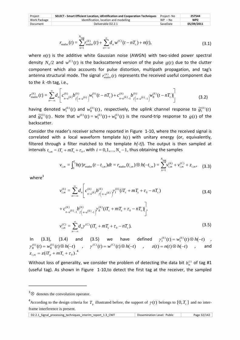
D2.2.1_Signal_processing_techniques_interim_report_1.3_CNIT Dissemination Level: Public Page 32/142
(3.2)
,)()()(=)( c
)C(
=
)(
reader
tag
1=
reader tnnTtwdtrtr n
n
k
N
k
where )(tn is the additive white Gaussian noise (AWGN) with two-sided power spectral
density /20N and )((C) tw is the backscattered version of the pulse )(tg due to the clutter
component which also accounts for pulse distortion, multipath propagation, and tag's antenna structural mode. The signal )()(
reader tr k represents the received useful component due
to the k -th tag, i.e.,
)()(=)( c
)(
II
)(
1)(
)(
1)(c
)(
I
)(
)(
)(
)(
=
)(
reader nTtwbcnTtwbcdtr kk
kunf
k
kun
kk
kunf
k
kun
n
n
k
having denoted )()(
I tw k and )()(
II tw k , respectively, the uplink channel response to )(~ )(
I tg k
and )(~ )(
II tg k . Note that )()(=)( )(
II
)(
I
)( twtwtw kkk is the round-trip response to )(tg of the
backscatter.
Consider the reader's receiver scheme reported in Figure 1-10, where the received signal is correlated with a local waveform template )(th with unitary energy (or, equivalently,
filtered through a filter matched to the template h(-t)). The output is then sampled at intervals
0sc, = TmTit mi, with 10,1,...,= s Ni , thus obtaining the samples
,=)()(=)()(= ,
)(
,
)(
,
tag
1=
,,reader,reader
c
0, mi
C
mi
k
mi
N
k
mimimi
T
mi zvvthtrdtttrthv
where3
)(= c0sc
)(
I
)(
)(
)(
)(
=
)(
, nTmTiTbcdv kk
kunf
k
kun
n
n
k
mi
,)( c0sc
)(
II
)(
1)(
)(
1)(
nTmTiTbc kk
kunf
k
kun
.)(= c0sc
)(
=
)(
, nTmTiTdv C
n
n
C
mi
In (3.3), (3.4) and (3.5) we have defined )()()( )(
I
)(
I thtwt kk ,
)()()( )(
II
)(
II thtwt kk , )()()( )C()C( thtwt , )()()( thtntz , and
)( 0sp, mTiTzz mi.4
Without loss of generality, we consider the problem of detecting the data bit (1)
mb of tag #1
(useful tag). As shown in Figure 1-10,to detect the first tag at the receiver, the sampled
3 denotes the convolution operator.
4According to the design criteria for
pT illustrated before, the support of )(t belongs to ][0, cT and no inter-
frame interference is present.
(3.1)
(3.3)
(3.4)
(3.5)
Project SELECT - Smart Efficient Location, idEntification and Cooperation Techniques Project- No 257544 Work Package Identification, location and modelling WP – No WP2 Document Deliverable D2.2.1 SaveDate 05/09/2011
D2.2.1_Signal_processing_techniques_interim_report_1.3_CNIT Dissemination Level: Public Page 33/142
signal miv ,
is multiplied by the composite sequence }{ (1)
nn dc , which identifies both the
reader and the desired tag #1.5 In particular, all sN resulting samples at the output of the
correlator composing a data symbol are summed up to form the m th decision variable at
the detector input. Considering that )()(
s= k
i
k
mNi cc , and imNi dd =
s
i , the decision variable
for the m -th symbol (1)
mb becomes
miii
N
i
m vdcy ,
(1)
1s
0=
=
(1)
1(1)
(1)
1(1)
(1)
0
2
00
(1)
II
(1)
(1)
(1)
(1)
(1)2
1s
0=
0
(1)
I )()(=
umfuumfuiii
N
i
bccdbccd
m
C
mmumfui
ii
N
i
zybccd
)((1)
1(1)
(1)
1(1)
(1)2
1s
1=
0
(1)
II )(
where
(1)
1s
0=
0
)(
c0sc
)(
=
(1)
1s
0=
)( )(=)(= i
N
i
CC
n
n
ii
N
i
C
m cnTmTiTdbcy
and miii
N
im zcdz ,
1s
0=
is a Gaussian distributed random variable (RV) with zero mean and
variance /2= 0s
2 NNz .
The component m accounts for the MUI and can be expressed as follows[10]
)(
,
(1)
1s
0=
tag
2=
= k
miii
N
i
N
k
m vdc
)(
1)(
)(
1)(
(1)
0
2
00
)(
II
)(
)(
)(
)(
(1)2
1s
0=
0
)(
I
tag
2=
)()(= k
kumf
k
ku
kk
kumf
k
kui
ii
N
i
k
N
k
bccdbccd
)(
1)(
)(
1)(
(1)2
1s
1=
0
)(
II )( k
kumf
k
kui
ii
N
i
k bccd
whose effect on the decision variable strictly depends on the cross-correlation property between codes }{ (1)
ic and }{ )(k
ic .
In the following we assume that code synchronization is achieved after an initial acquisition
phase, i.e., 0=(1)u . To this purpose a wake up signal available through the UHF part could
5Multiple readers may access the same tag by using different reader codes provided that they are designed with
good cross-correlation properties.
(3.6)
(3.7)
(3.8)
Project SELECT - Smart Efficient Location, idEntification and Cooperation Techniques Project- No 257544 Work Package Identification, location and modelling WP – No WP2 Document Deliverable D2.2.1 SaveDate 05/09/2011
D2.2.1_Signal_processing_techniques_interim_report_1.3_CNIT Dissemination Level: Public Page 34/142
(3.11)
archive this requirement enabling the possibility of avoiding complex acquisition techniques. From (3.6) we have
.)()()(= )((1)
1
(1)
0
(1)
10
(1)
II
(1)(1)
1
1s
1=
0
(1)
IIs0
(1)
I
(1)
m
C
mmmii
N
i
mm zybccccNby
Looking at (3.9) it can be noted that the useful term depends on the partial autocorrelation properties of code }{ (1)
ic .
As a further hypothesis we assume that a perfect TOA (Time of Arrival) estimate is available. Details on how the TOA estimated can be achieved are given in Sec. 3 and in [16]. Once the TOA is known, the reader can adjust its internal clock so that it becomes synchronous to that
of the intended tag, i.e., 0=(1) , and the optimal choice for 0 can be derived. In such a
case of perfect synchronization6
dttwE2
(1)
w0
(1)
I )(==)(
and (3.9) can be further simplified leading to
,== )(
s
(1))(
ws
(1)
mm
C
mmm
C
mmmm zyEbzyENby
where wss = ENE , and is the normalized cross-correlation between pulses )((1)
I tw and
)(th , which accounts for the mismatch due to pulse distortion. Parameters wE and
sE represent the average received energy per pulse and symbol, respectively.7 For further
convenience we define the SCR as cs
s=SCREN
E, where dttwE C
T 2)(p
0c )(= is the energy
per pulse of the clutter component.
3.2 Signal parameters design criteria
When choosing the signal parameters several constraints have to be taken into account.
The pulse repetition period Tp should be larger than the maximum backscatter delay, e.g., 133 ns means maximum 20 meters. This number does not affect tag’s parameters and can be changed on-the-fly by modifying Npc
6Note that under perfect timing condition it is )(=)( (1)(1)
I twtw and 0=)((1)
II tw . Moreover, as already
mentioned, any non ideal switching effect becomes negligible because it affects parts of the received signal not
interested by the useful backscattered pulse. 7Note that the energy of the useful tag response may vary for different delays and codes when the reader is not
synchronized. In such a case (22) does not hold anymore.
(3.9)
(3.10)
Project SELECT - Smart Efficient Location, idEntification and Cooperation Techniques Project- No 257544 Work Package Identification, location and modelling WP – No WP2 Document Deliverable D2.2.1 SaveDate 05/09/2011
D2.2.1_Signal_processing_techniques_interim_report_1.3_CNIT Dissemination Level: Public Page 35/142
The chip time Tc affects the tag power consumption [6] as well as the data rate together to the number of chips per data symbol Nc. Higher values of Tc reduce the tag consumption but also decrease the data rate.
As will be shown in section 3, high values of Npc reduce the sensitivity of the communication performance to tag clock drifts.
The communication performance is dominated by the total number of pulses per data symbol Ns=NcNpc. By increasing Ns the total SNR is increased as will be shown in section 3.3.3. However, the data rate Rb decreases correspondingly. Then there is a trade-off between performance in terms of bit error rate and data rate.
An example of realistic values for the parameters described in Table 1-2 is reported below:
Tc=1us Rc=1 Mchip/s
Nc=1024 Ts=1.024ms, Rb=976 bit/s
Npc=5 Tp=200ns (can be changed on-the-fly by the reader without requiring modifications at tag level)
3.3 Spreading codes design criteria
The aim of this section is to define the design criteria for the reader and tag spreading codes in order to allow multiple access of different tags and permit the clutter removal process necessary to detect the information bits. As reference we consider the example of Figure 1-1 related to the PAM backscatter modulation already treated in Sec. 2.2. Red waveforms are referred to the useful signal modulated in amplitude by the reader code (supposed in figure to be equal to one for all the pulses), the tag code and the data symbol, while green waveforms are related to the clutter modulated uniquely by the reader code.
Project SELECT - Smart Efficient Location, idEntification and Cooperation Techniques Project- No 257544 Work Package Identification, location and modelling WP – No WP2 Document Deliverable D2.2.1 SaveDate 05/09/2011
D2.2.1_Signal_processing_techniques_interim_report_1.3_CNIT Dissemination Level: Public Page 36/142
Figure 1-16 Example of PAM backscatter modulation format in case of Npc=1.
3.3.1 Clutter removal
Looking at (3.6), (3.7) and Figure 3-1, it can be noted that only the antenna mode scattered signals are modulated by the combination of the tag's and reader's codes }{ )(k
ic and }{ id ,
whereas all clutter signals components (including the antenna structural mode scattering) are received modulated only by the reader's code }{ id . This suggests, as can be deduced
from (3.7), that to completely remove the clutter component, and hence the antenna structural mode component, it is sufficient that the tag's code }{ (1)
ic has zero mean, i.e.,
0=(1)1s
0= n
N
nc
, leading to 0=)(C
my , if a quasi-stationary scenario within the symbol time sT is
assumed.
This behavior can be explained looking at Figure 1-17. After a coherent summation of the waveforms multiplied at the reader side by the zero-mean tag code, the clutter signals cancel out each other, assuming a stationary channel in the symbol time, while the useful components backscattered by the tag are coherently and in-phase summed up and the unique waveform polarity is due to the data bit transmitted in the current frame by the tag that the reader is detecting.
Project SELECT - Smart Efficient Location, idEntification and Cooperation Techniques Project- No 257544 Work Package Identification, location and modelling WP – No WP2 Document Deliverable D2.2.1 SaveDate 05/09/2011
D2.2.1_Signal_processing_techniques_interim_report_1.3_CNIT Dissemination Level: Public Page 37/142
Figure 1-17 Zero-mean tag code behavior.
3.3.2 Multiple access
Regarding the MUI, the situation is similar to what happens in conventional code division multiple access systems where the performance is strictly related to the partial cross-correlation properties of codes }{ (1)
ic and }{ )(k
ic . Classical codes such as Gold codes or m -
sequences offer good performance. Unfortunately they are composed of an odd number of symbols and hence there is no way to obtain a zero mean code to completely remove the clutter. However, considering that m -sequences have a quasi-balanced number of "+1" and "-1". i.e., their number differs no more than 1, one option to achieve clutter removal is to lengthen the code by one symbol so that the resulting code had zero mean. As a consequence we expect certain degradation in terms of multiple access performance, especially when short codes are adopted. In the numerical results this aspect will be investigated.
When the scenario is quasi-synchronous, i.e., 0=)(ku k and 0)( k , orthogonal codes, such as Hadamard codes, represent a good choice and 0=m . This could be the situation
where a wake up signal is sent by the reader to switch the tag on and reset the code phase. An extensive code behavior analysis will be object of further investigations.
3.3.3 Codes assignment strategies
One of the key that allows the proper functioning of the RFID UWB system is the codes behavior in order to permit multiple access and clutter removal. These codes have to be assigned to the tag. Different strategies are possible in order to archive this:
Project SELECT - Smart Efficient Location, idEntification and Cooperation Techniques Project- No 257544 Work Package Identification, location and modelling WP – No WP2 Document Deliverable D2.2.1 SaveDate 05/09/2011
D2.2.1_Signal_processing_techniques_interim_report_1.3_CNIT Dissemination Level: Public Page 38/142
• Option 1: the system assigns a unique code cn to each tag entering the area through the UHF link (login phase with a portal UHF reader/writer). Then all readers in the same area know the number of tags in the area and their respective cn.
• Option 2: each tag has a fixed cn code (e.g., fixed at manufacturing time) out of a small set of possible codes (e.g., 16 codes). No login phase is requested as all readers in the area are "tuned" on the 16 possible codes. Tags are distinguished because of the different unique ID transmitted as data. There is a high possibility of code collisions but, due to the extremely low duty cycle of the UWB transmission, the probability that collisions occur also in time should be low.
The first option, because of the login phase, requires a tighter interaction between the UWB and UHF parts of the tag for code assignment, and more flexibility at reader side as it has to be tuned to a larger set of different codes. The code length must be very large (>1000 for asynchronous scenarios). However, no data (ID) transmission between tag and reader is necessary as there is a unique correspondence between ID and spreading code. This fact implies a less stringent requirement on communication data rate as well as packet length and opens a new interesting scenario. In fact, in the extreme case, only the transmission of one bit is sufficient to detect the tag and hence the tag detection is concluded just after the acquisition phase (only preamble, no payload). In such a case, a simplified tag architecture is possible as shown in Fig. 4-3a, where no data memory is present and the spreading code can be changed through the UHF link. Since no data are transmitted, the most meaningful performance index is not anymore the bit error probability (BEP), but the probability of detection (Pd), i.e., the probability that the tag is detected, and the probability of false alarm Pf, i.e., the probability that, due to interference and noise, the tag is detected even if it is not present. The processing at the reader is simplified (no data demodulation) and the tag detection time is speeded up.
The second option does not necessary require a login phase and an interaction between the UWB and UHF tags. However, some performance degradation due to code collisions might be present. Shorter spreading codes can be adopted. Consequences of these possible collisions and related performance degradation, as well as synchronization issues, have to be studied with more detail in future.
Project SELECT - Smart Efficient Location, idEntification and Cooperation Techniques Project- No 257544 Work Package Identification, location and modelling WP – No WP2 Document Deliverable D2.2.1 SaveDate 05/09/2011
D2.2.1_Signal_processing_techniques_interim_report_1.3_CNIT Dissemination Level: Public Page 39/142
Figure 4-3a Alternative tag structure without payload
chip
UHF/UWB antenna
RFID modem
Power
management
control
batterycontrol logic
switch
m(t)
mem
ory
wake−up
UWB TAG
STANDARD UHF TAG
spread code
memory
{c }n
f
logic
In view of what emerged from the analysis presented the following considerations about code choice can be underlined:
• The tag’s code cn must have zero mean (equal number of +1 and -1) to remove the clutter during the de-spreading operation in the reader (in slow-varying channels). This requirement is less stringent if long codes are adopted (this will be analyzed in Section 3.3 through numerical results).
• The tag’s code cn can belong to an orthogonal codes set (e.g., Hadamard) if tags are quasi-synchronized through a wake-up signal. Up to Nc codewords (simultaneously detectable tags) are in this case available.
• The tag’s code cn must belong to PN-like code sets (e.g., Gold, m-sequences) if tags are not synchronized through a wake-up signal. Usually N<<Nc codewords (simultaneously detectable tags) are available, then very long codes are needed to support a large number of tags. For example adopting m-sequences with Nc =1023 we have only N=60 different codes. The number of codes increases to N=176 adopting a Nc =2047 m-sequence. Gold codes are obtained starting from the addition of two m-sequences and provides better cross-correlation properties but only a part of them is quasi-balanced (number of +1 and -1 that differs no more than 1).
Project SELECT - Smart Efficient Location, idEntification and Cooperation Techniques Project- No 257544 Work Package Identification, location and modelling WP – No WP2 Document Deliverable D2.2.1 SaveDate 05/09/2011
D2.2.1_Signal_processing_techniques_interim_report_1.3_CNIT Dissemination Level: Public Page 40/142
• Multiple readers can access simultaneously the same tag using different codes provided that they have good crosscorrelation properties (e.g., Gold codes if readers are asynchronous, orthogonal if readers are synchronous).
• If tags are asynchronous, code acquisition might take a very long time and synchronization algorithms could become highly complex.
• Data payload can be avoided if a login phase is foreseen and the system assigns a unique code cn to each tag entering the area (option 1).
3.3.4 Analysis of signal backscattered pulse quantization
Obviously, the quantization operation yields losses as regards to the backscattered pulse detection and then TOA estimation. In order to evaluate the impact of the quantization, a preliminary simulation study based on waveforms generated according to the IEEE 802.15.4a channel model has been carried out without accounting for the effect of clutter which deserves future investigations.
The quantization is done in full scale (without saturation) regarding the structural response for a tag-reader distance of 70 cm. No automatic gain control is considered. The quantization of the RF section output sample II, IQ, QI, QQ (see section 4.4) is done with 5 bits signed.
The TOA estimation is done on the antenna mode pulse scattering response, the tag is static, the channel is kept constant static during simulation (one realization of Residential LOS channel), code is 1023 length, and channel is Industrial LOS.
Project SELECT - Smart Efficient Location, idEntification and Cooperation Techniques Project- No 257544 Work Package Identification, location and modelling WP – No WP2 Document Deliverable D2.2.1 SaveDate 05/09/2011
D2.2.1_Signal_processing_techniques_interim_report_1.3_CNIT Dissemination Level: Public Page 41/142
Figure 1-18 Comparison of the quantized and not quantized channel energy profile at the output of the RF section. On the X-axis is the index of the energy bin, on the Y-index is the level of energy of the signal. The blue curve represents the RF output signal energy not quantized, whereas the red curve represents the RF output signal energy quantized
220 240 260 280 300 320 340 3600
2
4
6
8
10
12
x 10-3Comparison energy channel profile quantized vs non quantized - Rx-Tx distance : 1m
RF output signal energy
RF output signal energy quantized
220 240 260 280 300 320 340 360 3800
1
2
3
4
5
6
7
x 10-4 Comparison energy channel profile quantized vs non quantized - Rx-Tx distance : 2m
RF output signal energy
RF output signal energy quantized
a) tag-reader distance = 1m b) tag-reader distance = 2m
200 250 300 350 400 4500
1
2
x 10-4 Comparison energy channel profile quantized vs non quantized - Rx-Tx distance : 3 m
RF output signal energy
RF output signal energy quantized
240 260 280 300 320 340 360
1
2
3
4
5
6
7
8
9
10
11x 10
-5 Comparison energy channel profile quantized vs non quantized - Rx-Tx distance : 4m
RF output signal energy
RF output signal energy quantized
c) tag-reader distance = 3m d) tag-reader distance = 4m
200 250 300 3500
0.5
1
1.5
2
2.5
3
3.5
4
x 10-5 Comparison energy channel profile quantized vs non quantized - Rx-Tx distance : 4.5m
RF output signal energy
RF output signal energy quantized
e) tag-reader distance = 4,5 m
In the following table, the tag-reader maximum range that can be estimated versus the number of quantization bits has been summarized. The tag-reader maximum range is considered as the Tx-Rx distance for which the RF section output signal falls below the quantization step. It has to be remarked that these results do not account for the clutter
Project SELECT - Smart Efficient Location, idEntification and Cooperation Techniques Project- No 257544 Work Package Identification, location and modelling WP – No WP2 Document Deliverable D2.2.1 SaveDate 05/09/2011
D2.2.1_Signal_processing_techniques_interim_report_1.3_CNIT Dissemination Level: Public Page 42/142
(3.12)
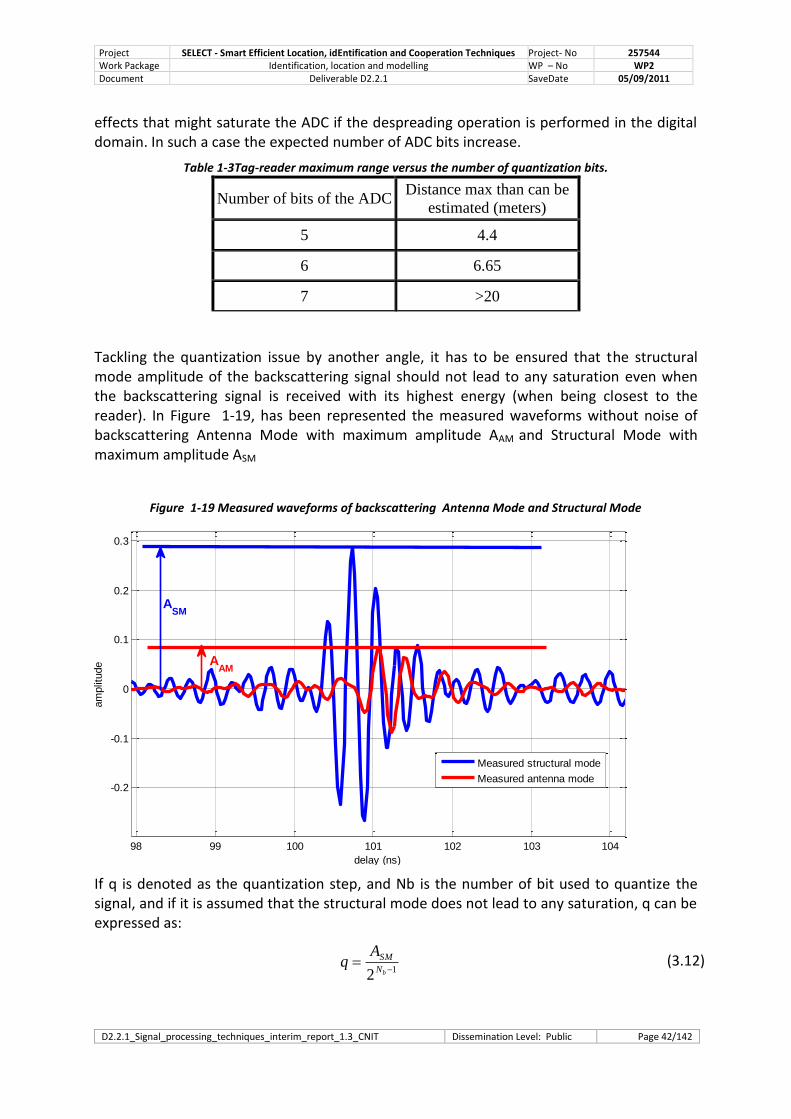
effects that might saturate the ADC if the despreading operation is performed in the digital domain. In such a case the expected number of ADC bits increase.
Table 1-3Tag-reader maximum range versus the number of quantization bits.
Number of bits of the ADC Distance max than can be
estimated (meters)
5 4.4
6 6.65
7 >20
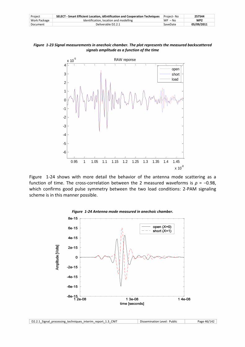
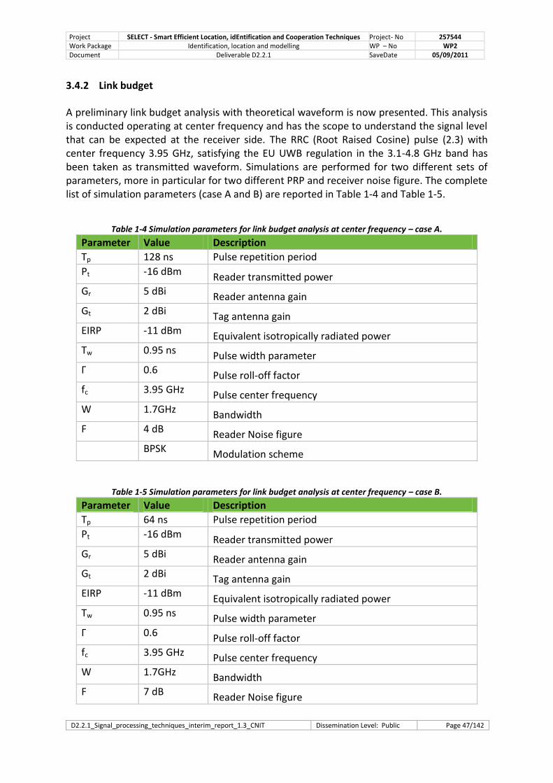
Tackling the quantization issue by another angle, it has to be ensured that the structural mode amplitude of the backscattering signal should not lead to any saturation even when the backscattering signal is received with its highest energy (when being closest to the reader). In Figure 1-19, has been represented the measured waveforms without noise of backscattering Antenna Mode with maximum amplitude AAM and Structural Mode with maximum amplitude ASM
Figure 1-19 Measured waveforms of backscattering Antenna Mode and Structural Mode
98 99 100 101 102 103 104
-0.2
-0.1
0
0.1
0.2
0.3
delay (ns)
am
plit
ude
Measured structural mode
Measured antenna mode
ASM
AAM
If q is denoted as the quantization step, and Nb is the number of bit used to quantize the signal, and if it is assumed that the structural mode does not lead to any saturation, q can be expressed as:
12
bN
SMAq
Project SELECT - Smart Efficient Location, idEntification and Cooperation Techniques Project- No 257544 Work Package Identification, location and modelling WP – No WP2 Document Deliverable D2.2.1 SaveDate 05/09/2011
D2.2.1_Signal_processing_techniques_interim_report_1.3_CNIT Dissemination Level: Public Page 43/142
(3.13)
(3.14)
The condition to ensure that the useful signal, the antenna mode signal, is quantized a minima is:
qAAM
The calculation is straightforward to give the minimum number of bits to quantize the signal:
1log 2
AM
SM
bA
AN
If using best cases values for AAM and ASM , we obtain :
3bN
3.3.5 Analysis of tag clock drift
The tag clock drift regards to the reader clock results in correlation losses at the reader side when correlating the backscattered code signal with the reference code. Another effect that might result in correlation losses is the reader-tag synchronization jitter. The importance of this effect is strictly correlated to the specific code adopted (e.g., orthogonal) and it is not accounted for in this section.
To evaluate the impact of this tag clock drift, two figures of merit have been computed:
- the ratio of the highest peak maximum amplitude of the ideal code autocorrelation over the highest peak maximum amplitude of the code correlation with code with drift. We call it here CPAPR : Cross-correlation Peak to Autocorrelation Peak Ratio.
- the ratio of the highest peak maximum amplitude of the code correlation with code with drift over the secondary max peak of correlation without main peak (peak of the code grass level) . We call it here CPGPR : Cross-correlation Peak to Grass Peak Ratio.
The CPAPR represents the pure correlation losses. The CPGPR represents the separation between code cross-correlation and code grass level, i.e. the increase ratio on the code synchronization false alarm probability.
These quantities have been evaluated for different parameters of signal structure:
- a 128 length code with 1 pulse per code chip
- a 128 length code with 8 pulse per code chip
- a 256 length code with 8 pulse per code chip
Project SELECT - Smart Efficient Location, idEntification and Cooperation Techniques Project- No 257544 Work Package Identification, location and modelling WP – No WP2 Document Deliverable D2.2.1 SaveDate 05/09/2011
D2.2.1_Signal_processing_techniques_interim_report_1.3_CNIT Dissemination Level: Public Page 44/142
Figure 1-20 Tag clock drift impact for a 1 x 128 code length.
0 0.5 1 1.5 2 2.5 3 3.5 4 4.5 50
0.1
0.2
0.3
0.4
0.5
0.6
0.7
0.8
0.9
1
Code clock Drift (in %)
maxim
um
s R
ati
oRatio of max peak amplitude of correlation function with drift
over max peak amplitude of correlation function without drift
Seq Length = 1 x 128, i.e. 1 pulse per chip code
0 0.5 1 1.5 2 2.5 3 3.5 4 4.5 50
1
2
3
4
5
6
7
8
9
10
Code clock Drift (in %)
maxim
um
s R
ati
o
Ratio of max peak amplitude of correlation function with drift
over max peak of the correlation function grass (without CF peak)
SeqLength = 1 x 128, i.e. 1 pulse per chip code
a) CPAPR b) CPGPR
Figure 1-21 Tag clock drift impact for a 8 x 128 code length.
0 5 10 15 20 25 30 35 40 45 500
0.1
0.2
0.3
0.4
0.5
0.6
0.7
0.8
0.9
1
Code clock Drift (in %)
maxim
um
s R
ati
o
Ratio of max peak amplitude of correlation function with drift
over max peak amplitude of correlation function without drift - Seq Length = 8 x 128
0 1 2 3 4 5 6 7 8 9 100
2
4
6
8
10
12
14
16
maxim
um
s R
ati
o
Code clock Drift (in %)
Ratio of max peak amplitude of correlation function with drift
over max peak of the correlation function grass (without CF peak) - SeqLength = 8 x 256
a) CPAPR b) CPGPR
If the limits are (very lowest limit) set to:
• -10dB correlation loss max on the CPAPR
• And min ratio of max main peak over grass max peak CPGPR is 1 (hard limit of code synchronization)
Then, the results obtained are:
• Clock drift limit for a 1x128 (only one pulse per code chip) sequence length is around 0.5%
• Clock drift limit for a 8x128 sequence length is around 5%
• Clock drift limit for a 8x256 sequence length is around 2%
We can thus conclude that against tag clock drift, it is beneficial to have several pulses per code chip. It is also possible to extrapolate the results for a 8x10²³ sequence: the tag clock drift limit should be in this case of around 0.5 %.
Project SELECT - Smart Efficient Location, idEntification and Cooperation Techniques Project- No 257544 Work Package Identification, location and modelling WP – No WP2 Document Deliverable D2.2.1 SaveDate 05/09/2011
D2.2.1_Signal_processing_techniques_interim_report_1.3_CNIT Dissemination Level: Public Page 45/142
Figure 1-22 Tag clock drift impact for a 8 x 256 code length.
0 1 2 3 4 5 6 7 8 9 100
0.1
0.2
0.3
0.4
0.5
0.6
0.7
0.8
0.9
1
Code clock Drift (in %)
maxim
um
s R
ati
o
Ratio of max peak amplitude of correlation function with drift
over max peak amplitude of correlation function without drift - Seq Length = 8 x 256
0 5 10 15 20 25 30 35 40 45 500
2
4
6
8
10
12
maxim
um
s R
ati
o
Code clock Drift (in %)
Ratio of max peak amplitude of correlation function with drift
over max peak of the correlation function grass (without CF peak) - SeqLength = 8 x 128
a) CPAPR b) CPGPR
3.4 Performance Analysis in the Reference Scenario
This section we show preliminary performance analysis conducted in ideal scenario (single tag, no multipath). First of all a link budget analysis will be presented in order to define the average received power taking in consideration the constraints of the FCC and EU UWB emission masks, to serve also as input for the work packages responsible for the reader and tag design.
Subsequently performance in terms of bit-error-rate and system constraints will be shown basing the analysis on theoretical waveforms and measured waveforms taken in anechoic chamber.
3.4.1 Preliminary measurements analysis in anechoic chamber
Figure 1-23 shows an example of measured backscattered signal at reference distance dref= 1.44 m, taken in anechoic chamber for different antenna load conditions (open-short). A BAV (Balanced Antipodal Vivaldi) antenna in the direction of maximum radiation is considered. Antenna mode scattering is divided by the structural mode scattering by means of a delay line (in a real system these two contributions will be received overlapped). As can be seen, the structural mode scattering is independent on the load condition while the antenna mode scattering is different in the case of open circuit, short circuit or matched load.
Project SELECT - Smart Efficient Location, idEntification and Cooperation Techniques Project- No 257544 Work Package Identification, location and modelling WP – No WP2 Document Deliverable D2.2.1 SaveDate 05/09/2011
D2.2.1_Signal_processing_techniques_interim_report_1.3_CNIT Dissemination Level: Public Page 46/142
Figure 1-23 Signal measurements in anechoic chamber. The plot represents the measured backscattered signals amplitude as a function of the time
0.95 1 1.05 1.1 1.15 1.2 1.25 1.3 1.35 1.4 1.45
x 10-8
-6
-5
-4
-3
-2
-1
0
1
2
3
4x 10
-5 RAW reponse
open
short
load
Figure 1-24 shows with more detail the behavior of the antenna mode scattering as a function of time. The cross-correlation between the 2 measured waveforms is ρ = −0.98, which confirms good pulse symmetry between the two load conditions: 2-PAM signaling scheme is in this manner possible.
Figure 1-24 Antenna mode measured in anechoic chamber.
Project SELECT - Smart Efficient Location, idEntification and Cooperation Techniques Project- No 257544 Work Package Identification, location and modelling WP – No WP2 Document Deliverable D2.2.1 SaveDate 05/09/2011
D2.2.1_Signal_processing_techniques_interim_report_1.3_CNIT Dissemination Level: Public Page 47/142
3.4.2 Link budget
A preliminary link budget analysis with theoretical waveform is now presented. This analysis is conducted operating at center frequency and has the scope to understand the signal level that can be expected at the receiver side. The RRC (Root Raised Cosine) pulse (2.3) with center frequency 3.95 GHz, satisfying the EU UWB regulation in the 3.1-4.8 GHz band has been taken as transmitted waveform. Simulations are performed for two different sets of parameters, more in particular for two different PRP and receiver noise figure. The complete list of simulation parameters (case A and B) are reported in Table 1-4 and Table 1-5.
Table 1-4 Simulation parameters for link budget analysis at center frequency – case A.
Parameter Value Description
Tp 128 ns Pulse repetition period
Pt -16 dBm Reader transmitted power
Gr 5 dBi Reader antenna gain
Gt 2 dBi Tag antenna gain
EIRP -11 dBm Equivalent isotropically radiated power
Tw 0.95 ns Pulse width parameter
Γ 0.6 Pulse roll-off factor
fc 3.95 GHz Pulse center frequency
W 1.7GHz Bandwidth
F 4 dB Reader Noise figure
BPSK Modulation scheme
Table 1-5 Simulation parameters for link budget analysis at center frequency – case B.
Parameter Value Description
Tp 64 ns Pulse repetition period
Pt -16 dBm Reader transmitted power
Gr 5 dBi Reader antenna gain
Gt 2 dBi Tag antenna gain
EIRP -11 dBm Equivalent isotropically radiated power
Tw 0.95 ns Pulse width parameter
Γ 0.6 Pulse roll-off factor
fc 3.95 GHz Pulse center frequency
W 1.7GHz Bandwidth
F 7 dB Reader Noise figure
Project SELECT - Smart Efficient Location, idEntification and Cooperation Techniques Project- No 257544 Work Package Identification, location and modelling WP – No WP2 Document Deliverable D2.2.1 SaveDate 05/09/2011
D2.2.1_Signal_processing_techniques_interim_report_1.3_CNIT Dissemination Level: Public Page 48/142
BPSK Modulation scheme
Figure 1-25 and Figure 1-26 show the transmitted RRC pulse taking in consideration the parameters presented in Table 1-4 and Table 1-5. The different amplitude is due to the different PRP. In fact the system is constrained by the emission mask regarding the radiated PSD: increasing the PRP leads to an increase of the pulse amplitude and, consequently, the pulse energy, maintaining the same EIRP value. The correspondent radiated PSD, taking into consideration the peak reader antenna gain, is reported in Figure 1-27: note that this PSD is the same for both the parameter sets (both case A and case B). The correspondent received power is reported in Figure 1-28 considering the free-space attenuation of a single path in presence of different losses due to the backscattering process in the tag (i.e. losses due to the presence of a not-ideal switch, delay lines,…). Also in this case, since the EIRP is the same and the reader antenna has the same gain, the power link budget results equal for cases A and B.
Figure 1-25 Transmitted pulse according to EU UWB regulation – case A.
Project SELECT - Smart Efficient Location, idEntification and Cooperation Techniques Project- No 257544 Work Package Identification, location and modelling WP – No WP2 Document Deliverable D2.2.1 SaveDate 05/09/2011
D2.2.1_Signal_processing_techniques_interim_report_1.3_CNIT Dissemination Level: Public Page 49/142
Figure 1-26 Transmitted pulse according to EU UWB regulation – case B.
Figure 1-27 Power spectral density of the radiated signal.
Project SELECT - Smart Efficient Location, idEntification and Cooperation Techniques Project- No 257544 Work Package Identification, location and modelling WP – No WP2 Document Deliverable D2.2.1 SaveDate 05/09/2011
D2.2.1_Signal_processing_techniques_interim_report_1.3_CNIT Dissemination Level: Public Page 50/142
Figure 1-28 Received power at the reader side.
Figure 1-29 Peak voltage at reader side – case A
Project SELECT - Smart Efficient Location, idEntification and Cooperation Techniques Project- No 257544 Work Package Identification, location and modelling WP – No WP2 Document Deliverable D2.2.1 SaveDate 05/09/2011
D2.2.1_Signal_processing_techniques_interim_report_1.3_CNIT Dissemination Level: Public Page 51/142
Figure 1-30 Peak voltage at reader side – case B
The peak voltage at the reader side is also plotted in Figure 1-29 and Figure 1-30Errore. L'origine riferimento non è stata trovata., where also the noise RMS level WRN0 (Volt),
with FkTN 00 and noise figure F=4 dB and 7 dB, is reported8.
Table 1-6 and Table 1-7 report the level of the useful signal in transmission and the level of the noise at the receiver according to parameters of Table 1-4 and Table 1-5.
Table 1-6 Signal and noise levels – case A.
Parameter Value Description
Pt -16 dBm Transmitted power
Vpeak 0.67 V Transmitted pulse peak amplitude
Ep 4.95e-10 V^2 s Transmitted pulse energy
N0 -110 dBm/MHz Noise PSD
Pn 17 pW Noise power in a band W=1.7 GHz
Vrms 29 uV Noise RMS value
Table 1-7 Signal and noise levels – case B.
Parameter Value Description
Pt -16 dBm Transmitted power
Vpeak 0.47 V Transmitted pulse peak amplitude
8k represent the Boltzmann constant, T0=290K the reference temperature and R=50Ω the load resistance.
Project SELECT - Smart Efficient Location, idEntification and Cooperation Techniques Project- No 257544 Work Package Identification, location and modelling WP – No WP2 Document Deliverable D2.2.1 SaveDate 05/09/2011
D2.2.1_Signal_processing_techniques_interim_report_1.3_CNIT Dissemination Level: Public Page 52/142
Ep 2.47e-10 V^2 s Transmitted pulse energy
N0 -107 dBm/MHz Noise PSD
Pn 34 pW Noise power in a band W=1.7 GHz
Vrms 41uV Noise RMS value
The single-pulse signal-to-noise ratio SNRp at the receiver side is reported in Figure 1-31 and Figure 1-32.
The dynamic range with respect to one meter, i.e. the ratio between the peak amplitude at one-meter distance and the generic peak amplitude at distance d, is reported in Figure 1-33: also this parameter, defined as a ratio, results independent on system parameters. Note that the final signal-to-noise ratio, SNR, at the demodulator is given by SNR=SNRp Ns. As a consequence, one approach to improve the SNR without increasing the transmitted power is to increase the number of pulses per symbol Ns by reducing the bit rate.
Figure 1-31 Single-pulse signal-to-noise ratio at the reader side – case A.
Project SELECT - Smart Efficient Location, idEntification and Cooperation Techniques Project- No 257544 Work Package Identification, location and modelling WP – No WP2 Document Deliverable D2.2.1 SaveDate 05/09/2011
D2.2.1_Signal_processing_techniques_interim_report_1.3_CNIT Dissemination Level: Public Page 53/142
Figure 1-32 Single-pulse signal-to-noise ratio at the reader side – case B.
Figure 1-33 Dynamic range at the reader side.
3.4.3 Data Rate and Bit Error Rate analysis
A first performance analysis, in terms of data rate – bit error rate, is here reported.
As receiver solution we consider two alternatives:
Single-path matched filter (SPMF)
In the absence of other information the matched filter (MF) template is chosen to be proportional to the received pulse in free-space propagation at the orientation of
Project SELECT - Smart Efficient Location, idEntification and Cooperation Techniques Project- No 257544 Work Package Identification, location and modelling WP – No WP2 Document Deliverable D2.2.1 SaveDate 05/09/2011
D2.2.1_Signal_processing_techniques_interim_report_1.3_CNIT Dissemination Level: Public Page 54/142
maximum tag’s antenna radiation. This receiver is optimal in AWGN but it is sub-optimal in a multipath scenario. In such a case, the receiver can easily be extended to obtain a Rake structure composed of a number
pL of fingers, each of them synchronized to a
different path.
Ideal Matched Filter (IMF)
The IMF receiver is a Rake receiver with unlimited correlators (all Rake Receiver) and a perfect estimate of the received waveform to be used as local template.
The performance of the SPMF, or any other receiver solutions such as those based on Rake structures, are bounded by the ideal matched filter (IMF) receiver which can be used as a benchmark solution. Both solutions suppose a coherent receiver with perfect synchronization.
We now present the performance in a single-tag and multi-tag scenarios in order to gain some insights about the attainable ultimate performance using the backscatter communication mechanism. In the absence of other tags in the environment we have
0=m , whereas clutter contribution is completely suppressed thanks to the adoption of
zero mean codes.
The performance in the ideal scenario can be obtained by
0
2
sb erfc
2
1=
N
EP
where )( erfc is the complementary error function and accounts for the mismatch
between the received signal and the template in the SPMF receiver. The performance of the
IMF can be easily obtained by setting 1
For further convenience, we define prefref /= EEG , i.e., the round-trip channel power gain at
the reference distance refd and at the maximum direction of radiation
maxΘ in AWGN
scenario, where refE is the received energy per pulse at the reference distance
refd and
pE the transmitted energy. In addition, we assume a typical exponential path loss law where
the power path loss exponent typically ranges between 1.8 and 4 . The bit error
probability can be rewritten as [12]
b0
2
ref2
reft
b erfc2
1=
RN
d
dGP
P
where )1/(= psb TNR is the data rate (symbol rate). It is interesting to note that the
exponent 2 is present instead of in (3.16) to account for the two-way link.
(3.15)
(3.16)
Project SELECT - Smart Efficient Location, idEntification and Cooperation Techniques Project- No 257544 Work Package Identification, location and modelling WP – No WP2 Document Deliverable D2.2.1 SaveDate 05/09/2011
D2.2.1_Signal_processing_techniques_interim_report_1.3_CNIT Dissemination Level: Public Page 55/142
(3.17)
Figure 1-34 shows the distance-data rate relation for single path matched filter (SPMF) in AWGN for different TAG orientation angles (BAV antenna considered), with target bit error probability 10-3. In this case waveforms taken by measurements conducted in anechoic chamber have been used.
Figure 1-34 Distance-Data rate relation for single path matched filter (SPMF) in AWGN for different TAG orientation angles, with target bit error probability 10
-3.
For what concerns the analysis conducted with signals in agreement with the EU UWB mask, the number of pulses, considering an AWGN channel, necessary to reach the SNR needed to assure the target bit error probability 10-3 (i.e. the number of pulses needed to reach the target SNR=6.79dB considering a matched filter) is reported in Figure 1-35 and Figure 1-36. The correspondent data rate is reported in Figure 1-37 and Figure 1-38.
As example if we consider a distance of 10 meters, looking at Figure 1-31 for 0dB tag losses, we notice that the single-pulse SNRp is near to -30 dB; since about 7 dB are required for a matched filter to reach the 10-3 BEP, a gain of 37 dB is required. This gain corresponds to about 5000 pulses, as visible in Figure 1-35.
For what concerns the receiver implementation, a strong limitation is given by the ADC dynamic: the number of quantization levels has to guarantee low distortion for the useful signal part without incurring in saturation due to the presence of the clutter component. The signal-to-quantization-noise-ratio (SQNR), i.e. the ratio between the signal power and the noise power introduced by the quantization process, can be calculated as
SQNR=E[X2 ]
M 23L2
Project SELECT - Smart Efficient Location, idEntification and Cooperation Techniques Project- No 257544 Work Package Identification, location and modelling WP – No WP2 Document Deliverable D2.2.1 SaveDate 05/09/2011
D2.2.1_Signal_processing_techniques_interim_report_1.3_CNIT Dissemination Level: Public Page 56/142
where M is the ADC dynamic, X is the random variable that represents the sampled signal, and L=2m is the number of quantization levels obtained using m bits. Considering the hardware proposed by LETI, presented in Figure 4.5, the digital conversion is operated after the correlation process. In order to evaluate the SQNR in necessary to characterize the statistics of the clutter falling within the integration window at the receiver, information not available at this moment. As first results we now assume to directly sample the waveform taking M as the maximum clutter amplitude and substituting E[X2] with the square of the signal peak amplitude. By inverting equation 3.17 it is possible to compute the maximum tolerable clutter amplitude M, for different numbers of ADC bits, corresponding to a minimum SQNR target of 10dB. These results are presented in Figure 3.25 and Figure 3.26. As an example let us suppose to work with the parameters of simulation case A: considering a reader-tag distance of 10m and assuming that the ADC digitalizes the signal using m=7 bits
(pink curve), the receiver works with SQNR10dB only if the clutter has a peak amplitude equal of less of 10-4 Volt.
Figure 1-35 Number of pulses necessary to reach the target BEP of 10-3
– case A.
0 1 2 3 4 5 6 7 8 9 10 11 12 13 14 1510
0
101
102
103
104
105
106
distance [m]
Ns
Tag loss: 0dB
Tag loss: 3dB
Tag loss: 5dB
Project SELECT - Smart Efficient Location, idEntification and Cooperation Techniques Project- No 257544 Work Package Identification, location and modelling WP – No WP2 Document Deliverable D2.2.1 SaveDate 05/09/2011
D2.2.1_Signal_processing_techniques_interim_report_1.3_CNIT Dissemination Level: Public Page 57/142
Figure 1-36 Number of pulses necessary to reach the target BEP of 10-3
– case B.
0 1 2 3 4 5 6 7 8 9 10 11 12 13 14 1510
0
101
102
103
104
105
106
distance [m]
Ns
Tag loss: 0dB
Tag loss: 3dB
Tag loss: 5dB
Figure 1-37 Data rate considering a target BEP of 10-3
- case A.
0 1 2 3 4 5 6 7 8 9 10 11 12 13 14 1510
2
103
104
105
106
distance [m]
Data
Ra
te (
bp
s)
Tag loss: 0dB
Tag loss: 3dB
Tag loss: 5dB
Project SELECT - Smart Efficient Location, idEntification and Cooperation Techniques Project- No 257544 Work Package Identification, location and modelling WP – No WP2 Document Deliverable D2.2.1 SaveDate 05/09/2011
D2.2.1_Signal_processing_techniques_interim_report_1.3_CNIT Dissemination Level: Public Page 58/142
Figure 1-38 Data rate considering a target BEP of 10-3
- case B.
0 1 2 3 4 5 6 7 8 9 10 11 12 13 14 1510
2
103
104
105
106
distance [m]
Data
Ra
te (
bp
s)
Tag loss: 0dB
Tag loss: 3dB
Tag loss: 5dB
Similarly, assuming from measurements that the clutter as a certain amplitude, it is possible to find, by looking at Figure 3.25 and Figure 3.26, the minimum number of required ADC bits
compliant with the requirement SQNR10dB at a given reader-tag distance.
Figure 1-39 Maximum clutter amplitude tolerable to have a minimum SQNR=10dB – case A.
Project SELECT - Smart Efficient Location, idEntification and Cooperation Techniques Project- No 257544 Work Package Identification, location and modelling WP – No WP2 Document Deliverable D2.2.1 SaveDate 05/09/2011
D2.2.1_Signal_processing_techniques_interim_report_1.3_CNIT Dissemination Level: Public Page 59/142
Figure 1-40 Maximum clutter amplitude tolerable to have a minimum SQNR=10dB – case B.
3.4.4 UHF link budget for wake-up signals
Since the utility of the wake up signal has been underlined a simple link-budget considering a UHF 866 MHz carrier frequency with ERP=2W is shown in Figure 1-41. For the calculation 1 dB tag’s antenna gain and free-space conditions are considered. In order to understand the maximum wake up distance, a careful analysis of the minimum received power required to trigger the circuit is need.
Figure 1-41 UHF link budget.
Project SELECT - Smart Efficient Location, idEntification and Cooperation Techniques Project- No 257544 Work Package Identification, location and modelling WP – No WP2 Document Deliverable D2.2.1 SaveDate 05/09/2011
D2.2.1_Signal_processing_techniques_interim_report_1.3_CNIT Dissemination Level: Public Page 60/142
3.5 Preliminary Performance Analysis in Real Environments
In this section we present some preliminary performance analysis based on measurements campaign realized in real indoor environments (for a more detailed description of the measurements see[4] and [11]).
3.5.1 Measurements set up
Figure 1-42 Measurements at ENSTA laboratory.
The backscattering signal from a UWB antenna was measured in a typical indoor environment at ENSTA-ParisTech laboratory. Measurements were performed in the frequency domain, by means of a vector network analyzer (VNA) in the 2-12GHz band with steps of 5MHz. Two Horn Lindgren 3117 antennas were employed as reference antennas. They were placed in a quasi-monostatic configuration, separated by 18cm, guaranteeing a high isolation between the transmit and receive channels as shown in Figure 1-42.
The scattering from a UWB Monopole Dual Feed Stripline (DFMS), which is a small planar
antenna, was measured. Its dimensions ( 3mm32440 ) make this antenna quite suitable
for RFID tags. Three different load conditions were considered.
In indoor environment, a rectangular grid of nine points as showed in Figure 1-43 spaced out of about 1m in depth and cm70 in width, was defined in a room with furniture and
having dimensions ( 2m4.495.13 ). The tag was positioned alternatively in each point on a
vertical support. For both cases, a simple data processing was performed to obtain the
antenna backscattering response from the measured 21S . The collected data was first
filtered in the frequency domain to avoid ringing effect. Then, applying the inverse Fourier transform, the signal in the time domain was derived.
Project SELECT - Smart Efficient Location, idEntification and Cooperation Techniques Project- No 257544 Work Package Identification, location and modelling WP – No WP2 Document Deliverable D2.2.1 SaveDate 05/09/2011
D2.2.1_Signal_processing_techniques_interim_report_1.3_CNIT Dissemination Level: Public Page 61/142
Figure 1-43 Indoor scenario considered for the measurement campaign at ENSTA-ParisTech. The distances between each point and the antennas connected to the VNA are also reported.
VNA
1m
A B C
G H I
D E F
0.7m1m
A B C
G H I
D E F
0.7m
TX RX
dA=1.30m dD=2.22m
dE=2.12m
dG=3.16m
dH=3.10mdB=1.10m
dC=1.31m dF=2.26m dI=3.15m
In Figure 1-44an example of backscattered signal received from the tag placed at point H (distance 3.10m) is reported. As can be noted several clutter components (including the antenna structural mode) are present.
The second plot shows the antenna mode backscattered signal (that of interest) after clutter removal. Due to its small amplitude (about 2 orders of magnitude less than the clutter) it results to be completely buried below the clutter component.
Then clutter and the antenna structural mode scattering have a significant impact at the reader's antenna, thus making the detection of the antenna mode scattered signal (which carries data) a main issue in passive UWB RFID systems.
Project SELECT - Smart Efficient Location, idEntification and Cooperation Techniques Project- No 257544 Work Package Identification, location and modelling WP – No WP2 Document Deliverable D2.2.1 SaveDate 05/09/2011
D2.2.1_Signal_processing_techniques_interim_report_1.3_CNIT Dissemination Level: Public Page 62/142
Figure 1-44 Example of the laboratory impulse response (grid point H, at distance of 3.1 m) and of the antenna mode contribution (after clutter removal).
3.5.2 Bit error probability analysis
3.5.2.1 Performance in AWGN and single-tag laboratory scenario
We now present the bit error probability of the UWB-RFID system as a function of the data rate
bR . The transmitted pulse shape and power have been chosen so that the transmitted
signal is compliant with the 3.1-10.6 GHz FCC mask. Specifically, the 6th derivative Gaussian
monocycle has been considered. The other parameters are 100=fT ns and the effective
isotropically radiated power is 6.70= EIRP dBm. Results related to the SPMF receiver in
AWGN channel (obtained using measurement data in anechoic chamber considering a distance 1.46=d m) and in every grid point location inside the laboratory are shown in
Figure 1-45 and Figure 1-46 respectively[10].
Project SELECT - Smart Efficient Location, idEntification and Cooperation Techniques Project- No 257544 Work Package Identification, location and modelling WP – No WP2 Document Deliverable D2.2.1 SaveDate 05/09/2011
D2.2.1_Signal_processing_techniques_interim_report_1.3_CNIT Dissemination Level: Public Page 63/142
Figure 1-45 Bit error probability as a function of the bit rate in different tag locations. SPMF receiver is considered.
As expected, the performance of the IMF receiver is significantly better than that obtained using the simple SPMF receiver because all useful energy coming from multipath is captured and hence the performance depends only on the received power. In fact, the SPMF receiver is not able to collect the energy from multipath and suffers from pulse distortion due to propagation as well as antenna effects. The problem can be mitigated by considering more complex receiver structures, such as those based on Rake solutions. The performance obtained with the tag located at point B is better than AWGN condition because of the shorter distance (1.10 m vs 1.46 m). It can be noted that in some cases tags placed at larger
distances correspond to higher performance. This result depends on the higher amount of energy that can be collected in some locations due to the presence of richer multipath.
If we fix the target bit error probability (e.g. 3
b 10= P ), results show that data rates up to
200 kbit/s at a distance of 3.10 m with a transmitted power lower than 1 mW are feasible in
a realistic environment. It is important to remark that similar performance is achievable by the conventional UHF RFID technology only using a transmitted power higher than 1 W (i.e.,
more than 3 orders of magnitude higher level).
Project SELECT - Smart Efficient Location, idEntification and Cooperation Techniques Project- No 257544 Work Package Identification, location and modelling WP – No WP2 Document Deliverable D2.2.1 SaveDate 05/09/2011
D2.2.1_Signal_processing_techniques_interim_report_1.3_CNIT Dissemination Level: Public Page 64/142
Figure 1-46 Bit error probability as a function of the bit rate in different tag locations. IMF is considered.
3.5.2.2 Performance in multi-tag scenario with artificial clutter
We now show the BER in the presence of interfering tags as a function of the SIR. The SNR
has been fixed to 7 dB, corresponding to an error floor of about 310 in the absence of
interference. Results have been obtained by Monte Carlo simulations starting from antenna backscatter measurements in anechoic chamber. The interfering tag, the clutter and the thermal noise signal components have been added artificially according to the set SNR, SIR, and SCR values. The clutter waveform has been taken from measurements in the laboratory environment. The worst case scenario with the interfering signal completely overlapped to the useful one is considered.
In Figure 1-47 results associated to different spreading codes are compared. In the quasi-synchronous scenario orthogonal Hadamard codes are used[10]. As expected the performance is not sensitive to the presence of both the interference and clutter (because of the zero-mean code used). In the asynchronous scenario m -sequences spreading codes of length 7 and 63 have been considered. From the curve corresponding to m -seq 7 it can be observed that when clutter is present and significative ( 79=SCR dB), even for large SIR
values, the performance is limited by the clutter. A remarkable improvement can be obtained by extending the length of the code by one (zero-mean code). When longer codes are used (e.g., m -seq 63) the impact of clutter becomes less significant and good performance can be achieved even using non zero-mean codes. These considerations suggest that the adoption of extended m -sequences is an interesting choice, especially when working with short code sequences.
Project SELECT - Smart Efficient Location, idEntification and Cooperation Techniques Project- No 257544 Work Package Identification, location and modelling WP – No WP2 Document Deliverable D2.2.1 SaveDate 05/09/2011
D2.2.1_Signal_processing_techniques_interim_report_1.3_CNIT Dissemination Level: Public Page 65/142
Figure 1-47 BER as a function of the SIR in the anechoic chamber scenario where clutter is summed up artificially.
3.5.2.3 Performance in multi-tag laboratory scenario
In Figure 1-48 the BER as a function of the SNR when 6=tagN tags are present is reported
[10]. The signal measured from the location D of the grid is considered as the signal backscattered by the useful tag, and then we associate the backscattered signals coming from locations A, B, C, E, F (see the map in Figure 1-43) to the interfering signals. Different SNR values have been obtained by adding the correspondent artificial thermal noise.
It is possible to see the performance gain obtained when the extended m -sequence 63 is adopted. This indicates that the effect of the clutter is dominant with respect to the effect of the MUI. A similar conclusion can be drawn when only one interfering tag located in F is present and an extended m -sequence 7 is considered.
Project SELECT - Smart Efficient Location, idEntification and Cooperation Techniques Project- No 257544 Work Package Identification, location and modelling WP – No WP2 Document Deliverable D2.2.1 SaveDate 05/09/2011
D2.2.1_Signal_processing_techniques_interim_report_1.3_CNIT Dissemination Level: Public Page 66/142
Figure 1-48 BER as a function of SNR (Laboratory scenario).The useful tag is located in point D. Five interfering tags are present in locations A,B,C,E,F when m-sequence 63 is adopted. One interferer tag in location F is considered when m-sequence 7 is used.
3.6 Concluding remarks
The frame design has been determined as regards to the tag and reader architecture and the system performance. It impacts the refresh rate of the TOA measurements, the SNR at the reader through the acceptable signal coherent integration time, and the multi-tag access capability via specific spreading codes.
Parameters value choice has to be taken as a trade off of several contrasting effects. The key parameter by means of which the performance vs data rate trade-off can be determined is the total number of pulses per symbol Ns.
The adoption of backscatter modulation and the extremely low transmitted power levels, correspond to a poor link budget that limits the transmission range. Moreover the dominant effect of the clutter imposes severe constrains on the ADC resolution.
In order to extend the transmission range, the SNR should be increased via long duration signal coherent integration. Preliminary numerical results show that operating ranges up to 15-20 meters are feasible in AWGN with a sufficiently large Ns. Good performance can also be achieved in realistic scenarios with multipath even using SPMF receivers. Several pulses per code chip are needed to minimize the effect of the tag clock drift on the TOA estimation.
Zero-mean codes allow removing the clutter components as expected. This requirement of zero-mean codes usage is less stringent adopting long codes. The code length should be well
Project SELECT - Smart Efficient Location, idEntification and Cooperation Techniques Project- No 257544 Work Package Identification, location and modelling WP – No WP2 Document Deliverable D2.2.1 SaveDate 05/09/2011
D2.2.1_Signal_processing_techniques_interim_report_1.3_CNIT Dissemination Level: Public Page 67/142
chosen in order to mitigate the clutter impact on the ranging accuracy and to decrease the multiple access interference.
Results confirm the superior performance of orthogonal codes with respect to PN codes: the former is applicable to a quasi-synchronous system, i.e., readers and tags must be synchronized with an error not larger than the chip time. This requires the adoption of a wake-up strategy using the UHF down-link able to guarantee low wake-up time jitter.
However, a more detailed study is necessary in order to define the performance expected in case of multi tag and multi reader scenario using different types of codes.
Project SELECT - Smart Efficient Location, idEntification and Cooperation Techniques Project- No 257544 Work Package Identification, location and modelling WP – No WP2 Document Deliverable D2.2.1 SaveDate 05/09/2011
D2.2.1_Signal_processing_techniques_interim_report_1.3_CNIT Dissemination Level: Public Page 68/142
4 Signal Processing Techniques for Ranging
The ranging technique choice is of paramount importance since it has a crucial impact on the overall system tag localization accuracy. In the SELECT framework, since the requirement on localization accuracy is stringent and the link budget of backscattered pulse is poor, a TOA-based ranging technique is adopted. In this section, we first describe the signal generation and propagation model used, then few considerations about PHY layer are developed, the receiver front-end architecture is presented. Then, the TOA estimation algorithm chosen is investigated, and finally, TOA estimation performance is showed.
4.1 Theoretical bound on TOA estimation
In an ideal scenario characterized by AWGN, the theoretical limit on the mean square TOA estimation error is given by the Cramer-Rao Lower Bound (CRLB). For a generic pulse of shape p(t) it is given by:
SNRCRLB
228
1
with
dffP
dffPf
2
22
2
)(
)(
where SNR is the signal to noise ratio per pulse and β represents the effective bandwidth of the pulse. )( fP is the spectrum of p(t). Then as can be seen, to improve the TOA estimation
accuracy (and hence ranging accuracy), it is beneficial to adopt very large bandwidth signals (e.g., UWB) and improve the SNR. The latter can be achieved by energy accumulation through the transmission of several pulses.
Figure 1-49 shows the CRLB and Ziv-Zakai bounds for TOA estimation RMSE using RRC and Gaussian pulses [65].
(4.1)
Project SELECT - Smart Efficient Location, idEntification and Cooperation Techniques Project- No 257544 Work Package Identification, location and modelling WP – No WP2 Document Deliverable D2.2.1 SaveDate 05/09/2011
D2.2.1_Signal_processing_techniques_interim_report_1.3_CNIT Dissemination Level: Public Page 69/142
Figure 1-49 CRLB and Ziv-Zakai bounds for TOA estimation RMSE using RRC and Gaussian pulses.
4.2 Signal generation and propagation model
The signal generation and propagation model is detailed in deliverable [4], but the main features are here recalled.
The channel model is derived from antenna backscattering measurements. A backscattered UWB pulse is measured in anechoic chamber for different angle of arrival. This measured pulse waveform is then convolved with a Channel Impulse Response (CIR) which is generated using a dynamic channel model preserving IEEE 802.15.4a statistics described in [7]. In this analysis, Wire-Patch antenna measurements are used. An example of a measured backscatter pulse at 0° angle is displayed in Figure 1-50. Figure 1-51 represents an example of an industrial LOS type CIR realization. The result of the convolution of the pulse by the CIR is plotted in Figure 1-52.
Project SELECT - Smart Efficient Location, idEntification and Cooperation Techniques Project- No 257544 Work Package Identification, location and modelling WP – No WP2 Document Deliverable D2.2.1 SaveDate 05/09/2011
D2.2.1_Signal_processing_techniques_interim_report_1.3_CNIT Dissemination Level: Public Page 70/142
Figure 1-50 Backscattered pulse measured in anechoic chamber-wire patch antenna.
-10 -5 0 5 10-0.1
-0.05
0
0.05
Delay (in ns)
Am
plitu
de
Backscattering pulse waveform
Figure 1-51 Example of a realization of the channel - dynamic channel model -CM1.
0 0.2 0.4 0.6 0.8 1 1.2 1.4
x 10-7
-0.4
-0.2
0
0.2
0.4
0.6
Delay (in s)
Am
plitu
de
Channel - Residential LOS
Project SELECT - Smart Efficient Location, idEntification and Cooperation Techniques Project- No 257544 Work Package Identification, location and modelling WP – No WP2 Document Deliverable D2.2.1 SaveDate 05/09/2011
D2.2.1_Signal_processing_techniques_interim_report_1.3_CNIT Dissemination Level: Public Page 71/142
Figure 1-52 Example of backscattering CIR obtained with the proposed channel model.
0 50 100 150 200 250-0.04
-0.03
-0.02
-0.01
0
0.01
0.02
0.03
0.04
Delay (in ns)
Am
plitu
de
Pulse after convolution with channel
and backscattering waveform
At the beginning of the simulation, a realization of the CIR is computed. Then, at each instant, depending on the relative location of the backscattering tag regarding the transmitting reader, the CIR evolves dynamically respecting the IEEE 802.15.4a statistics. At each instant, each ray composing the CIR is associated with the correct backscattered pulse measurement which is dependent on the angle of arrival, to result in the received signal at the reader. The overall signal path loss is proportional to the tag-reader distance at the exponent 4 (as remarked in [4]) since the signal emitted by the reader is simply backscattered by the tag before being received by the reader.
4.3 PHY layer considerations
As analyzed in section 3, the frame design is determined as regards to the system performance. It impacts the refresh rate of the TOA measurements, the SNR at the reader through the acceptable signal coherent integration time, and the multi-tag access capability via specific spreading codes.
Specifically, the preamble during which several symbols are repeated should be long enough to enable the signal synchronization process. The symbol duration during the preamble should be sufficiently extended to permit a long coherent integration time to increase the Signal to Noise Ratio (SNR). The spreading code should be used to enables tag multiple access capability and to remove the clutter. The code length should be well chosen in order to mitigate the clutter impact on the ranging accuracy and to decrease the multiple access interference as shown in section 3. Finally, several pulses per code chip are needed to minimize the effect of the tag clock drift on the TOA estimation.
An example of a frame format that could be correctly designed to meet the system requirements is displayed in Figure 1-53.
Project SELECT - Smart Efficient Location, idEntification and Cooperation Techniques Project- No 257544 Work Package Identification, location and modelling WP – No WP2 Document Deliverable D2.2.1 SaveDate 05/09/2011
D2.2.1_Signal_processing_techniques_interim_report_1.3_CNIT Dissemination Level: Public Page 72/142
Figure 1-53Frame format example.
PreamblePreamble128 bits128 bits
ID Code128 bits
Spreading CodeSpreading Code1023 bits1023 bits
512 ms
Tbit = 2 ms
Tchip = 2 us
PRP = 256 ns8 pulses Tag Clock @ 500kHz
T Tag Clock ≈ T Chip
PreamblePreamble128 bits128 bits
ID Code128 bits
Spreading CodeSpreading Code1023 bits1023 bits
512 ms
Tbit = 2 ms
Tchip = 2 us
PRP = 256 ns8 pulses Tag Clock @ 500kHz
T Tag Clock ≈ T Chip
4.4 Receiver architecture
The proposed receiver front-end is based on the architecture of a UWB low power receiver developed at CEA-LETI. The architecture of this RF front-end is detailed in the following.
The incoming signal is first down-converted to base-band and low pass filtered. A second mixer is then used to translate the signal on an intermediate frequency. This operation is done in order to project the signal on a sinusoidal basis, which makes a refined TOA estimation possible. Successively, the signal is integrated over one IF sinusoid period, which is here equal to 2ns. The four channel output signals II, IQ, QI, QQ are finally digitized with a 5bits ADC at 62.5 MHz. The actual ADC resolution appears to be not sufficient to satisfy the requirements shown in section 3.3.4. Then the possibility to extend/change the ADC will be investigated in the following up research activity.
The index of the integrators, i.e. the time position of the integration window, must be controlled by an external digital circuit. The windows are 50% overlapped (i.e. one start of 2 ns window integration every 1 ns). Additionally, hardware constraints impose to have at ones disposal four windows available per 64 ns period.
Project SELECT - Smart Efficient Location, idEntification and Cooperation Techniques Project- No 257544 Work Package Identification, location and modelling WP – No WP2 Document Deliverable D2.2.1 SaveDate 05/09/2011
D2.2.1_Signal_processing_techniques_interim_report_1.3_CNIT Dissemination Level: Public Page 73/142
Figure 1-54 UWB RF front-end architecture.
LNA
Low pass filter
tunable cut-off frequency:
250 1200 MHz
Low pass filter
tunable cut-off frequency:
250 1200 MHz
ADC5 bits
ADC5 bits
II
IQ°
°
Indexes of the 2ns integration
windows
62.5 MHz
4 GHz
62.5 MHz
°
°
ADC5 bits
ADC5 bits
QI
QQ
Indexes of the 2ns integration
windows
62.5 MHz
62.5 MHz
°
°
500 MHz
The four digitized sampled signals - II, IQ, QI, QQ - are correlated with the reference code at digital processing level, and then squared and summed up together. From this operation, the signal energy present in each integration windows is computed. A threshold detection test over the energy signal present in each integrated windows enables the signal coarse TOA estimation.
4.5 Synchronization process
Before being able to estimate the TOA of the signal, the frame synchronization has to be realized. The synchronization is done during the preamble of the frame. The aim is to determine in which time windows are located the signal pulses and which window corresponds to the start of the data payload which is here the tag’s ID code.
Taking into account the RF Front-end hardware constraints, the synchronization algorithm performs circular correlation of the received signal with the reference code (with a given tag-reader code dn cn). The highest value of this correlation and its position (window index) is stored if this value exceeds a threshold. During this processing, for each integration window position within a pulse repetition period (i.e. code period), a new circular correlation is computed and compared to the threshold. The process stops when 2 same positions for windows index have been found in two successive laps of the algorithm.
4.6 TOA Estimation algorithms
In the SELECT framework, harsh signal propagation conditions have to be faced. The received pulse signal which energy is low due to the backscattering is affected by noise, dense multipath and strong clutter. Even in LOS conditions, the TOA-based ranging can be biased. Thus, specific TOA estimation algorithm has to be employed.
Project SELECT - Smart Efficient Location, idEntification and Cooperation Techniques Project- No 257544 Work Package Identification, location and modelling WP – No WP2 Document Deliverable D2.2.1 SaveDate 05/09/2011
D2.2.1_Signal_processing_techniques_interim_report_1.3_CNIT Dissemination Level: Public Page 74/142
The TOA estimation is done in two steps. First, a coarse estimation that determines the integration windows index corresponding to the TOA, leading to a 1ns precision. Second, a refined TOA estimation is performed within the window, leading to a theoretical 125 ps precision. 125 ps is the precision limit induced by the hardware design of the analog front-end and the digital signal processing implementation choices (e.g. atan look-up table implementation, etc....
4.6.1 TOA coarse estimation
The TOA estimation algorithm described in [19] appears to be of particular interest in our context. This leading edge TOA signal estimation algorithm has demonstrated good multipath mitigation performance ([18], [19]). The main features of this algorithm are illustrated in Figure 1-55.
This detection test algorithm is done on the signal energy kz where,
kz is expressed as
follows:
2222
kkkkk QQQIIQIIz
where II, IQ, QI, QQ, are the RF front-end digitized output samples after correlation with the reference code mentioned in previous section.
Each rectangular bin in Figure 1-55 represents a k-index window of energykz .
Once the channel is estimated, the highest energy window has to be found. The TOA search process begins from the index of this highest energy window. It continues backward on the sample index scale, till the following dual condition: the energy of the current tested sample exceeds a threshold and the D successive following samples has energy below this threshold.
Analytically, the window index corresponding to the estimated leading edge TOA is expressed by the relation:
SBWnDkk
kSB
TOA zzand
zWnnnkn
max,max1
max1maxmax
,....max
/,....,,max
where
is the threshold to which are compared the energy samples
SBW is the index window (i.e. number of index) which limits the backward search
maxnis the index of the highest signal energy window
D is the number of samples backwardly tested successive to the current tested
energy sample
(4.2)
(4.3)
Project SELECT - Smart Efficient Location, idEntification and Cooperation Techniques Project- No 257544 Work Package Identification, location and modelling WP – No WP2 Document Deliverable D2.2.1 SaveDate 05/09/2011
D2.2.1_Signal_processing_techniques_interim_report_1.3_CNIT Dissemination Level: Public Page 75/142
Figure 1-55 Serial Backward Search for Multiple Cluster TOA algorithm principles illustration.
1 2 3 Sample indexK
Threshold ξ
nTOA nmax
Wsb : search back window
1 2 3 Sample indexK
Threshold ξ
nTOA nmax
Wsb : search back window
The threshold adopted is given by [19]:
edD
FAed PQ
11 11
where Q() is the Gaussian Q-function, ed is the energy signal
kz standard deviation
ed is the mean of the energy signal kz .
FAP is the false alarm probability
The value of the search back window SBW is linked to the statistics of the channel. In our
case, it has been chosen equal to the RMS delay spread. The chosen value for the parameter D, result of simulations, is chosen equal to 7. As discussed in [18], these parameters are typically determined in an empirical way. The false alarm probability is an application-dependent parameter. Typically values ranges from 0.1% to 1%.
It has been shown in [18] that, for high SNR values, a simple threshold comparison algorithm can lead to higher estimate accuracy than the SBS-MC algorithm. Consequently, these two algorithms are combined. Along the simulations, the SNR is estimated. If the SNR exceeds a fixed value (in our case chosen to 25 dB), the simple threshold comparison output is used as the TOA estimate. If the SNR is below this fixed value, the SBS-MC algorithm is used as the TOA estimate.
4.6.2 TOA refined estimation
The front-end architecture presented in 4.4 enables with the presence of the second mixer onto an IF, the computation of a refined estimate of the TOA. Once the TOA coarse estimate is obtained, the refined estimate is computed within the corresponding window of index k as follows:
2222
2222
arctan
arctan
kkkk
k
k
kkkk
k
k
FINE
QIQQIIIQifQI
QQ
QIQQIIIQifII
IQ
TOA
(4.4)
(4.5)
Project SELECT - Smart Efficient Location, idEntification and Cooperation Techniques Project- No 257544 Work Package Identification, location and modelling WP – No WP2 Document Deliverable D2.2.1 SaveDate 05/09/2011
D2.2.1_Signal_processing_techniques_interim_report_1.3_CNIT Dissemination Level: Public Page 76/142
4.7 Performance Analysis in the Reference Scenario
It is assumed that the reference scenario is defined by tags located in a square cell of 10m x 10m area with four readers at the corner of this square at 2m height. In this context, TOA estimation simulation has been done for a tag-reader distance from 1m to 12m. The signal generation and propagation model of section 4.2 has been used. Two IEEE802.15.4a channel has been considered: Residential LOS (CM1) and Industrial LOS (CM7). The front-end architecture presented in section 4.4 is modeled and employed in the simulation. The frame synchronization process is assumed to be successfully realized. The TOA estimation is done as described in section 4.6.1 and 4.6.2.
The emitted signal power is equal to -10dBm. The length of the spreading code is fixed to Nc=1023 chips with Npc=8 pulses per chip, and it is assumed that the coherent integration is realized over the duration corresponding to the length of the code.
It is assumed that no tag clock drift affects the TOA estimation process and no quantization is done on the received backscattered signal. These impairments will be analyzed in the next research activity, however these results are still important as they provide a sort of benchmark which different implementation can be compared to.
In this section, since the simulation are done for a tag considered static, for each realization of the TOA estimation, a new IEEE802.15.4a channel independent from the previous ones has been drawn.
Two metrics have been retained: the localization error outage and the ranging error standard deviation.
4.7.1 Ranging error outage
The ranging error outage is a metric defining the integrity of the process. It can also be used here to characterize the ranging estimation performance. This metric is expressed by:
thexeREO )(Pr
with e(x) being the TOA estimate error.
eth is a fixed ranging error threshold
It represents the probability for the ranging error to exceed a fixed error threshold.
Figure 1-56 shows the error outage resulting of a simulation using the CM1 channel for several tag-reader distances. For each tag-reader distance from 1m to 12m, the tag is set static and 2000 realizations of the ranging estimation process have been drawn.
(4.6)
Project SELECT - Smart Efficient Location, idEntification and Cooperation Techniques Project- No 257544 Work Package Identification, location and modelling WP – No WP2 Document Deliverable D2.2.1 SaveDate 05/09/2011
D2.2.1_Signal_processing_techniques_interim_report_1.3_CNIT Dissemination Level: Public Page 77/142
Figure 1-56 Ranging error outage as a function of the error threshold for CM1 channel.
0 0.2 0.4 0.6 0.8 1 1.2 1.4 1.6
0
20
40
60
80
100
error threshold - th
(in m)
ran
gin
g e
rro
r o
uta
ge
(in
%)
ranging error outage function of error threshold - CM1 Channel
Tx-Rx distance = 1m
Tx-Rx distance = 2m
Tx-Rx distance = 3m
Tx-Rx distance = 4m
Tx-Rx distance = 5m
Tx-Rx distance = 6m
Tx-Rx distance = 7m
Tx-Rx distance = 8m
Tx-Rx distance = 9m
Tx-Rx distance = 10m
Tx-Rx distance = 11m
Tx-Rx distance = 12m
It can be noticed here that for a tag-reader distance below 9m, a 25% REO is achieved for an estimate error below 20 cm. For tag-reader distance values higher than 9m, the error increases significantly.
Figure 1-57 shows the error outage resulting of a simulation using the CM7 channel for several tag-reader distances. For this Industrial LOS channel simulation, it can be observed that the performance is much decreased. A 25% REO is achieved for an estimate error below 45 cm for a tag-reader distance below 8m.
Project SELECT - Smart Efficient Location, idEntification and Cooperation Techniques Project- No 257544 Work Package Identification, location and modelling WP – No WP2 Document Deliverable D2.2.1 SaveDate 05/09/2011
D2.2.1_Signal_processing_techniques_interim_report_1.3_CNIT Dissemination Level: Public Page 78/142
Figure 1-57 Error outage as a function of the error threshold for CM7 channel.
0 0.5 1 1.5 2 2.5 3 3.5 4 4.5 5
0
10
20
30
40
50
60
70
80
90
100
error threshold - th
(in m)
Ra
ng
ing
Err
or
ou
tag
e -
LE
O (
in %
)ranging error outage function of error threshold - CM7 channel
Tx-Rx distance = 1m
Tx-Rx distance = 2m
Tx-Rx distance = 3m
Tx-Rx distance = 4m
Tx-Rx distance = 5m
Tx-Rx distance = 6m
Tx-Rx distance = 7m
Tx-Rx distance = 8m
Tx-Rx distance = 9m
Tx-Rx distance = 10m
Tx-Rx distance = 11m
Tx-Rx distance = 12m
4.7.2 Ranging error standard deviation
For this simulation, the tag-reader distance varies from 1m to 13m. Each step of 1m represents 500 realizations of the ranging estimation process.
The Root Mean Square Error (RMSE) of the TOA-based ranging estimation has been plotted for Residential LOS (CM1) and Industrial LOS (CM7) on Figure 1-58.
It can be noticed that the TOA-based ranging error stays below 30 cm in the operational range of [0 m, 8 m]. However, it is expected that the presence of quantization effects would degrade the performance.
Project SELECT - Smart Efficient Location, idEntification and Cooperation Techniques Project- No 257544 Work Package Identification, location and modelling WP – No WP2 Document Deliverable D2.2.1 SaveDate 05/09/2011
D2.2.1_Signal_processing_techniques_interim_report_1.3_CNIT Dissemination Level: Public Page 79/142
Figure 1-58 Ranging RMSE as a function of the tag-reader distance for CM1 and CM7 channels.
2 4 6 8 10 120
0.1
0.2
0.3
0.4
0.5
0.6
0.7
0.8
0.9
TOA estimation RMSE
Tag-Reader distance (m)
Ra
ng
ing
err
or
sta
nd
ard
de
via
tio
n (
m)
CM1
CM7
4.7.3 Concluding remarks
In this section, the CEA-LETI analog front-end design has been described. The digital signal processing envisioned to be developed in this framework has been detailed. The performance of the TOA-based ranging estimation has been analyzed.
It can be concluded that for a CM1 channel, the SELECT requirement in terms of accuracy is almost fulfilled. For CM7 channel, Industrial LOS channel, it is not the case, and improvements in terms of ranging estimation still have to be made (optimization of the estimation thresholds, etc…) to meet the requirements even if the localization/tracking module will obviously enable to enhance the location accuracy.
Project SELECT - Smart Efficient Location, idEntification and Cooperation Techniques Project- No 257544 Work Package Identification, location and modelling WP – No WP2 Document Deliverable D2.2.1 SaveDate 05/09/2011
D2.2.1_Signal_processing_techniques_interim_report_1.3_CNIT Dissemination Level: Public Page 80/142
5 Signal processing Techniques for Localization
This section describes models, algorithms, and performance results for localization and tracking of tagged and untagged objects in single cell and multicell scenarios of interest.
5.1 Preliminaries
Network localization and navigation represents a new paradigm where wireless networks support data communication, contextual information collection, and navigation. The purpose of such networks is to determine the unknown positions of agents based on intra- and inter-node measurements. In conventional approaches such as in the global positioning system (GPS), each agent infers its position using only measurements made with respect to anchors (nodes with a priori position knowledge belonging to the infrastructure). Such systems usually fail in harsh environments where network coverage is limited and measurements behavior is highly complex [61]. The localization and navigation process typically consists of two phases: (i) a measurement phase, during which agents make intra- and inter-node measurements using different sensors; (ii) a location-update phase, during which agents infer their own positions using an algorithm that incorporates both prior knowledge of their positions and new measurements. For instance, an agent can update its position estimate based on inertial measurements using an inertial measurement unit (IMU) and distance measurements with respect to some fixed anchors using a range measurement unit (RMU). The localization accuracy strongly depends on the quality of the measurements, which are affected by impairments such as network topology, multipath propagation, environmental conditions, interference, noise, and clock drift. In addition to the underlying technologies used in the measurement phase, the localization performance is also dependent on the specific processing or data fusion algorithm used in the location-update phase. Hence, a deep understanding of information evolution in different phases of the localization process is necessary for the design and analysis of localization systems.
5.2 Localization performance metrics
The requirements of location-aware networks are driven by applications. A local performance metric is the position estimation error (localization error) given by the Euclidean distance between the estimated position and the true position as
.
The root mean squared error (RMSE) of position estimates is then given by
where and are the estimated and true positions respectively.
A global performance metric evaluated over the entire localization area and time is the localization error outage (LEO) defined by
(5.1)
(5.2)
(5.3)
Project SELECT - Smart Efficient Location, idEntification and Cooperation Techniques Project- No 257544 Work Package Identification, location and modelling WP – No WP2 Document Deliverable D2.2.1 SaveDate 05/09/2011
D2.2.1_Signal_processing_techniques_interim_report_1.3_CNIT Dissemination Level: Public Page 81/142
where is the target (i.e., the maximum allowable) position estimation error, and the probability is evaluated over the ensemble of all possible spatial positions and time instants. Other requirements include localization update rate (i.e., the number of position estimates computed per second) and coverage area of the localization system. In particular, localization update rate is important for navigation (navigation of pedestrians and vehicles typically requires different localization update rates), which drives algorithm complexity and node cost.
5.3 Theoretical Foundation
Understanding the fundamentals theoretical limits (performance bounds) of localization and navigation systems is important not only to provide performance benchmarks when assessing the performance of any practical algorithms, but also to guide algorithm development and network design. In this section we illustrate a general framework for the evaluation of the theoretical bounds in a generic localization scenario where nodes with unknown positions (we refer to agents for the sake of generality) try to estimate their position. To be as general as possible, we consider the possibility that agents could also cooperate each other [62], [63], [64].
Consider a network with fixed nodes (anchors) and agents, where each agent is equipped with multiple sensors that can provide intra- and inter-node measurements (e.g., using IMU and RMU, respectively) for the purpose of localization and navigation. Using these intra- and
inter-node measurements, represented by , the agents aim to infer their
positions . The accuracy of location estimates is inherently limited due to random phenomena affecting , and fundamental limits of such accuracy have been derived using the information inequality [61], [64].
For a static network, or a dynamic network at a given time instant, only the spatial cooperation among the agents can be exploited. By using the notion of equivalent Fisher information matrix (EFIM)[65], the squared position error for agent is bounded by
where is the EFIM for [as depicted in Fig. 5.1(b)], and are the
expectation and trace operators, respectively, and denotes the square submatrix on the diagonal corresponding to . The right-hand side is referred to as the squared position error
bound (SPEB). It can be shown that the EFIM is a sum of two parts, the localization information from anchors (show as block-diagonal matrices consisting of ’s in Fig. 5.1) and that from agents’ spatial cooperation (shown as the structured matrix consisting of ’s in Fig.
5.1). The basic building blocks of the EFIM represent the localization information
between pairs of nodes in the form , where is the unit vector with direction given
(5.4)
Project SELECT - Smart Efficient Location, idEntification and Cooperation Techniques Project- No 257544 Work Package Identification, location and modelling WP – No WP2 Document Deliverable D2.2.1 SaveDate 05/09/2011
D2.2.1_Signal_processing_techniques_interim_report_1.3_CNIT Dissemination Level: Public Page 82/142
by denoting the angle from one node to the other, and is a positive scalar that characterizes the ranging information intensity (RII) [65]. The value of depends on the ranging technique as well as the power and bandwidth of the received waveform, multipath propagation, and prior statistical channel knowledge. In particular, the RII is proportional to the square of the effective bandwidth [65]. Moreover, the localization information from anchors can be expressed in a canonical form as a weighted sum of “one-dimensional” information from individual anchors; while cooperation always improves the localization accuracy since it adds a positive semi-definite matrix to the EFIM corresponding to non-cooperative localization. It was shown in [65]that the accuracy of localization is affected by two factors: the quality of point-to-point measurements, reflected by the expression of RII,
and the network topology, reflected by the block structure of the matrix . In the
absence of cooperation, every corresponding to cooperation between nodes and
becomes , resulting in a total EFIM with block-diagonal structure [as depicted in Fig. 5.1]. In such cases, localization information for different agents are uncorrelated, and the SPEB can be calculated using only local information at the agents.
Building on the understanding of cooperative localization, we now discuss the case of cooperative navigation where agents in a dynamic network cooperate in both space and time domains. For each time instant, the contribution of cooperation in space is similar to what we have seen in cooperative localization. In addition, another layer of cooperation in time, exploiting intra-node measurements and mobility (dynamic) models, yields new information for navigation. Such information is characterized by matrices in the total EFIM
as depicted in Fig. 5.1, where consists of the positions of all agents from time 1 to . Consequently, the SPEB for each agent at a given time instant can be obtained by a formula similar to (1). Some observations can be drawn from the structure of the EFIM for cooperative navigation in Fig. 5.1. First, the total EFIM consists of two major components, the cooperation in space as well as in time. The former characterizes the localization information from inter-node measurements in the entire network at each time instant (shown as the diagonal block matrices); and the latter characterizes the information from intra-node measurements and mobility models at each individual agent (shown as components outside the main block-diagonal). Second, since intra-node measurements and the mobility models for different agents are independent, the corresponding matrices form a block diagonal matrix in the upper-right and lower-left quarter of the total EFIM. Third, the components can be viewed as the temporal link which connects localization information from spatial cooperation of the previous time instant to the current one. If the temporal link is not available (i.e., components are zero) then the total EFIM is block diagonal, implying that position inference is independent from time to time. The structure of the EFIM for cooperative navigation allows a recursive method to calculate the EFIM at each time instant. This view also provides insights into the information evolution of spatio-temporal cooperation in cooperative navigation.
Project SELECT - Smart Efficient Location, idEntification and Cooperation Techniques Project- No 257544 Work Package Identification, location and modelling WP – No WP2 Document Deliverable D2.2.1 SaveDate 05/09/2011
D2.2.1_Signal_processing_techniques_interim_report_1.3_CNIT Dissemination Level: Public Page 83/142
Figure 1-59 EFIM structures and corresponding Bayesian networks for three agents: (a) noncooperative localization, (b) spatial cooperation, and (c) spatio-temporal cooperation for two time steps.
17
K 1
K 2
K 3
K 1
K 2
K 3
−C12
−C12
−C13
−C13
−C23
−C23
−C112
−C112
−C113
−C113
−C123
−C123
−C212
−C212
−C213
−C213
−C223
−C223
K 11
K 12
K 13
K 21
K 22
K 23
T 121
T 121
T 122
T 122
T 123
T 123
x1
x1
x1
x1
x2
x2
x2
x2
x3
x3
x3
x3
z1
z1
z1
z1
z2
z2
z2
z2
z3
z3
z3
z3
z12
z12
z12
z13
z13
z13
z21
z21
z23
z23
z23
z32
z32
z32
z31
z31
z31
z11
z22
z33
z21
Time 1 Time 2
Time 1
Time 2
(a) Noncooperative
(b) Spatial
(c) Spatio-temporal
localization
cooperation
cooperation
Fig. 2. EFIM structures and corresponding Bayesian networks for three agents: (a) noncooperative localization, (b) spatial
cooperation, and (c) spatio-temporal cooperation for two time steps.
5.4 Reference scenarios for localization and tracking
As discussed in[2], two different scenarios have been considered for the localization and tracking. First, a single cell squared scenario of dimension 10 m with four readers located in the corners has been considered for the localization of a single tagged object. Two multicells scenarios are considered for the tracking, such as deterministic trajectory (conveyor belt) and stochastic trajectory (random walking). These scenarios are composed of a certain number of squared cells of dimension 5 m with four readers in the corners of each cell, as depicted in Figure 5.3.
The conveyor belt shown in Figure 5.4 is defined by four points of coordinates in meters A={-10,-15}, B={-10,0}, C={10,0}, D={10,15} a Cartesian coordinate system having origin in the center of the multicell scenario is assumed. The random walking coordinates at time k
are statistically determined as
where R is the localization update rate and
(5.5)
Project SELECT - Smart Efficient Location, idEntification and Cooperation Techniques Project- No 257544 Work Package Identification, location and modelling WP – No WP2 Document Deliverable D2.2.1 SaveDate 05/09/2011
D2.2.1_Signal_processing_techniques_interim_report_1.3_CNIT Dissemination Level: Public Page 84/142
and, for instance, θ = π or θ = π/3. We denoted with the Gaussian distribution with mean µ and standard deviation σ, and with U[a,b] the uniform distribution in the interval [a,b].An example of random walking is shown in Figure 5.5.
Figure 1-60 Single cell scenario.
Figure 1-61Conveyor Belt.
Figure 1-62 Multicell scenario.
Figure 1-63Random Walking.
(5.6)
Project SELECT - Smart Efficient Location, idEntification and Cooperation Techniques Project- No 257544 Work Package Identification, location and modelling WP – No WP2 Document Deliverable D2.2.1 SaveDate 05/09/2011
D2.2.1_Signal_processing_techniques_interim_report_1.3_CNIT Dissemination Level: Public Page 85/142
5.5 Localization and Tracking techniques
The task of network localization and tracking algorithms is to determine positions from measurements (observations) and prior knowledge. For TOA –based localization and tracking techniques, the objects positions are determined from TOA estimations of signals exchanged with readers. The main difference between the case of tagged and that of untagged objects is on TOA estimation which depends on hardware and signal processing. At a layer above on top of TOA estimation localization and tracking techniques operate independently of the nature of the objects. Hence, in the following we will summarize localization and tracking techniques in an unified way for tagged and untagged objects.
5.5.1 TOA estimation model for localization and tracking algorithms
The measured TOA for the transmitter to target to receiver path is affected by an error caused by additive white Gaussian noise and the propagation environment in which the system is operating. In general, we can model the TOA error as a Gaussian distributed
random variable where the mean takes into account the presence of positive bias in obstructed path conditions, and it can be considered zero in line-of-sight (LOS) conditions[65]. The standard deviation depends on the propagation environment, hardware dependent factors altering TOA measurements and received SNR. The estimated TOA results in
The presence of TOA error makes the real target position not yet belonging to the detection ellipse/circle for each transmitter/receiver pair. Thus, detection ellipses/circles intersection, if still existing, define a wrong position estimation resulting in a localization error. To conduct a performance analysis, the knowledge of the relation between and is needed. The function on is in general non-increasing and can be defined as
The function depends on the hardware solution for TOA estimation. If an energy detector is employed[65], it is possible to distinguish three different SNR values intervals. The regions of small and large SNR values respectively correspond to regions of large and
small standard deviation . The SNR at a single receiver is given by
(5.7)
(5.8)
Project SELECT - Smart Efficient Location, idEntification and Cooperation Techniques Project- No 257544 Work Package Identification, location and modelling WP – No WP2 Document Deliverable D2.2.1 SaveDate 05/09/2011
D2.2.1_Signal_processing_techniques_interim_report_1.3_CNIT Dissemination Level: Public Page 86/142
where is the number of pulses combined to perform a TOA estimation, is the power received per pulse, is the pulse repetition frequency (PRF), and denotes the one-side noise power spectral density (PSD).
For moderate SNR values a transition zone of standard deviation between the upper and lower levels is experienced. The upper and lower levels of respectively depend on the
observation and integration time of the energy detector as follows
Figure 5.6 shows a real example of suggested by measurements.
Figure 1-64 Example of derived in the FP7 European Project EUWB.
We now obtain the received SNR for a generic scenario of NT transmitter and NR receivers. In the case of monostatic readers, transmitters and receivers are co-located.
5.5.2 Maximum Likelihood Localization
Once ranging measurements are conducted at each receiver detecting the target, the estimated position is determined by localization algorithms elaborating the measurements. Thus, the localization accuracy depends on the localization algorithm adopted. In the following we will focus on maximum likelihood (ML) estimator that select the estimated target position maximizing a TOA likelihood function which depends on the statistics of TOA
(5.9)
(5.10)
Project SELECT - Smart Efficient Location, idEntification and Cooperation Techniques Project- No 257544 Work Package Identification, location and modelling WP – No WP2 Document Deliverable D2.2.1 SaveDate 05/09/2011
D2.2.1_Signal_processing_techniques_interim_report_1.3_CNIT Dissemination Level: Public Page 87/142
estimation error. The ML algorithm examines all the possible target position and, for Gaussian distributed TOA estimation error, determines the estimated position as follows
In addition, measurements can be refined contrasting the presence of non-zero mean errors (e.g. bias caused by the presence of walls) and reducing the impact of zero mean noise by averaging over several measurements as in active localization systems [66]. In many cases the ML approach could lead to high complexity algorithms, the often sub-optimal schemes may be preferred [29].
5.5.3 Tracking: Bayesian filters
Recursive Bayesian estimation is a general probabilistic approach for estimating an unknown probability density function (PDF) over time using incoming measurements and a mathematical process model. It enables the probabilistic estimation of a system dynamic state from noisy observations. The state can be a simple 2D position or a complex vector including, for instance, 3D position, pitch, roll, yaw, linear and rotational velocities [67]. We consider the estimation of the 2D position of the target (system state) at a given time slot ,
represented by the random variable (RV) , starting from inter-node intra-node
measurements (observations). Denote the set of position-dependent measurements collected at time slot . The time interval between 2 consecutive
observations is . At each time slot, a probability distribution over , called belief,
, represents the uncertainty. The Bayesian filter sequentially estimates such beliefs over the state space conditioned on all information contained in the sensed data. To
illustrate, we denote the sequence of time-indexed sensor observations . The
belief is then defined by the posterior density over the random variable conditioned on all sensor data available at time
.
From a posteriori PDF it is possible to determine the most probable state at time
given the history of the observations . The complexity grows with the time, because the number of measurements of the sensors grows over time unless a window of a given number of previous states is considered. To make the computation tractable, we assume that the dynamic system is a first-order Markov system, that is the window length is one and
the current state variable contains all relevant information for position updating. For locating objects, the Markov assumption implies that sensor measurements depend only on the current physical location of the agent and that the location at time depends only on
the previous state . Given the at time , the Belief at time is
(5.11)
(5.12)
(5.13)
Project SELECT - Smart Efficient Location, idEntification and Cooperation Techniques Project- No 257544 Work Package Identification, location and modelling WP – No WP2 Document Deliverable D2.2.1 SaveDate 05/09/2011
D2.2.1_Signal_processing_techniques_interim_report_1.3_CNIT Dissemination Level: Public Page 88/142
where the term is the mobility model for the agent, that gives the
probability to be in given the fact that it was in . Once a new observation
(measurement) is available at time , and the state estimation is updated as
where . Now we can calculate the new Belief function
where is the perceptual model which provides the probability to observe
given the position . The structure of Bayesian filter is reported in Figure 1-65. For location estimation, the perceptual model is usually considered a property of a given sensor technology and captures an error characteristics of the sensor. The implementation of
Bayesian filters requires the specification of the perceptual model , mobility
model , and the computation of the belief . Different
implementations of Bayesian filters differ in the representation of PDF for each state In particular, we consider the efficient suboptimal implementation via Particle Filter (PF).
Figure 1-65 Structure of a Bayesian filter.
(5.14)
(5.15)
Project SELECT - Smart Efficient Location, idEntification and Cooperation Techniques Project- No 257544 Work Package Identification, location and modelling WP – No WP2 Document Deliverable D2.2.1 SaveDate 05/09/2011
D2.2.1_Signal_processing_techniques_interim_report_1.3_CNIT Dissemination Level: Public Page 89/142
Mobility Models:
A common way to model the mobility uncertainties is through the Gaussian distribution, i.e.,
where the variance accounts for the uncertainty in the movements and depends
on as will be shown in the following. We evaluate two mobility models which will be adopted in the numerical results to asses the performance of the tracking algorithm.
Mobility without direction information M1: in this case the PDF corresponds to a Gaussian distribution centered in
where it is assumed that the speed intensity is known and the speed direction is uniformly
distributed between .
Mobility with speed learning M2: in this model the speed is evaluated from previously estimated positions in a sliding window of length
Perceptual models
Assuming a 2D motion of the object and considering independent identically distributed observations, the perceptual model can be defined as
where is the observation at time . The perceptual model for each observation is assumed Gaussian distributed, that is,
(5.16)
(5.17)
(5.18)
(5.19)
(5.20)
Project SELECT - Smart Efficient Location, idEntification and Cooperation Techniques Project- No 257544 Work Package Identification, location and modelling WP – No WP2 Document Deliverable D2.2.1 SaveDate 05/09/2011
D2.2.1_Signal_processing_techniques_interim_report_1.3_CNIT Dissemination Level: Public Page 90/142
where is the position of anchor node from which the measure comes. The
variance depends on the technology used for localization. For example the model introduced in section 5.5.1 can be adopted.
5.5.4 Tracking: Particle filters
PFs compute the Belief update according to a sampling procedure, which is often referred to as sequential importance sampling with re-sampling. The key advantage of PFs is their ability to represent arbitrary PDF efficiently by automatically focusing their resources (particles) on regions in state space with high probability. The PF implementation requires attention when applied to high-dimensional estimation problem since the complexity grows exponentially with the dimension of the state space.
PFs are based on sets of samples weighted distributed according to the belief
approximated as
where is the number of particles, is the weight for particle at time , and
. The quality of the approximation depends on the number of particles [67]. To decrease the complexity, a non-uniform distribution of samples can be considered (e.g., more dense in the regions where it is more probable that the object is located). The sequential importance sampling (SIS) technique allows to extract samples from a PDF based on their importance. The a posteriori PDF is then approximated by weighted samples as
where is the Delta pseudo-function.
Since the is not known, a proposal distribution is chosen such that it can be factorized
and allows a recursive computation of the weights
(5.21)
(5.22)
(5.23)
(5.24)
Project SELECT - Smart Efficient Location, idEntification and Cooperation Techniques Project- No 257544 Work Package Identification, location and modelling WP – No WP2 Document Deliverable D2.2.1 SaveDate 05/09/2011
D2.2.1_Signal_processing_techniques_interim_report_1.3_CNIT Dissemination Level: Public Page 91/142
PFs typically adopt the following approximation
which transforms (1) into
The SIS algorithm has a drawback: after several iterations only few particles have a weight which is not negligible [68].To overcome this problem a resampling is done aiming to delete the inconsistent samples (those who have negligible weights) and increase the number of particles with high weights. This procedure is known as sequential importance resampling (SIR).
5.5.5 Tracking: Extended Kalman Filter
The Extended Kalman Filter (EKF) yields to optimal solutions of parameter estimation problem in a linear Gaussian context. In our framework (non linear, non Gaussian channel), Extended Kalman filtering is sub-optimal but remains still a very efficient solution for localization and tracking objects. We assume that the location tracking of the tag is performed in two dimensions.
The state (associated to the object) estimation is realized through a classical two step prediction-correction process. This implies to set an evolution model for the state, to define which the system’s observables are, and how the state and the observables are linked. It is detailed in the following developments how the EKF formalism can be adapted to our location estimation context.
The state model equation is given by:
kkk WXFX 1
where kX is the state vector describing the dynamic state of the tag at instant k
F is the state transition matrix from instant k-1 to instant k, setting the dynamic linear evolution model
kW is the state noise vector
The state vector is expressed as follows:
Tk
Y
k
X
k
X
k
X
kk
k AAVVyx ][)()()()()()(X
(5.25)
(5.26)
(5.27)
(5.28)
Project SELECT - Smart Efficient Location, idEntification and Cooperation Techniques Project- No 257544 Work Package Identification, location and modelling WP – No WP2 Document Deliverable D2.2.1 SaveDate 05/09/2011
D2.2.1_Signal_processing_techniques_interim_report_1.3_CNIT Dissemination Level: Public Page 92/142
where )()( , kk yx , )()(,
k
X
k
X VV , and )()(,
k
Y
k
X AA are respectively the position , speed,
and acceleration components of the tag.
The state noise vector is given by:
Tk
A
k
A
k
V
k
V
k
y
k
xk YXYXwwwwww ][
)()()()()()(W
where v
k
y
k
x Nww ,0,)()( is the position coordinate noise; v
k
V
k
V NwwYX
,0,)()( is
the speed coordinate noise, and a
k
A
k
A NwwYX
,0,)()( is the acceleration coordinate
noise. It is assumed that these noise processes are independent, and thus not correlated. Therefore, the state covariance matrix is diagonal, given by:
A
A
V
V
P
P
T
kkk E
0
0
WWQ
The state transition matrix F represents the predicted evolution of the state, and the noise
process kW is the incertitude relative to this prediction.
In our implementation, the state transition matrix F is expressed by:
100000
010000
01000
001002
10010
02
1001
2
2
dt
dt
dtdt
dtdt
F
where dt is the refresh rate of the filter.
The Kalman filter implements an observation vector with an associated observation model.
The observation vector kZ is composed of system measurement which enables the
correction of the predicted state.
The observation equation is expressed as:
kkk H VXZ )(
where kV represents the measurement noise vector at instant k.
In the chosen configuration, observations are composed of four values obtained from four TOAs, which are measured with respect to the four closest readers positioned at known positions. Thus, the observation vector is :
Tk
R
k
R
k
R
k
Rk zzzz ][)(
4
)(
3
)(
2
)(
1Z
(5.29)
(5.30)
(5.31)
(5.32)
(5.33)
Project SELECT - Smart Efficient Location, idEntification and Cooperation Techniques Project- No 257544 Work Package Identification, location and modelling WP – No WP2 Document Deliverable D2.2.1 SaveDate 05/09/2011
D2.2.1_Signal_processing_techniques_interim_report_1.3_CNIT Dissemination Level: Public Page 93/142
Where )(k
Rizis the round-trip time-of-flight measurement at instant k of the i-th reader’s
transmitted signal.
The non-linear function )(H in the observation equation links the state to each
measurement via the following relation:
)(2)()(2)()()( 1
,4,...,1k
Ri
k
Ri
kk
Ri
kk
Ri vyyxxc
zi
where )()(,
k
Ri
k
Ri yx are the coordinates of the i-th reader, )(k
Riv is the
measurement noise process assumed Gaussian and centered with the diagonal measurement covariance matrix being given by:
4
3
2
1
z
z
z
z
T
kkk E
0
0
VVR
In the chosen implementation, the standard deviation of the TOA estimation error given by a simplified model, which has been empirically fitted to simulations :
CRLBi mzi ,4,...,1
m represents the intrinsic precision of the TOA estimation associated with to the
receiver architecture. In our application: m = 125 ps (fixed parameter since it
represents the intrinsic limitation of the hardware). is tuned regarding simulation results
of section 4. The CRLB expression is given in section 4.1 where 2 is computed numerically
according to measured received pulses in anechoic chamber.
We assume that the state noise and observation noise are independent processes, and that
the initial state 0X is a vector independent of kV and kW .
We define 1/ˆ
kkX as an a priori state prediction at step k given knowledge of the process
from instant 0 to instant k-1, and kk /X̂ as an a posteriori state estimate at step k given
observations at instant k.
The a priori estimate error covariance matrix is defined by :
])ˆ()ˆ[( 1/1/1/
T
kkkkkkkk E XXXXP
Similarly, the a posteriori estimate error covariance matrix is given by :
])ˆ()ˆ[( ///
T
kkkkkkkk E XXXXP
The non-linear measurement function )(H is linearized around 1/ˆ
kkX through a Taylor
series, assuming that the derivate components from 2nd order are negligible:
(5.34)
(5.35)
(5.36)
(5.37)
(5.38)
(5.39)
Project SELECT - Smart Efficient Location, idEntification and Cooperation Techniques Project- No 257544 Work Package Identification, location and modelling WP – No WP2 Document Deliverable D2.2.1 SaveDate 05/09/2011
D2.2.1_Signal_processing_techniques_interim_report_1.3_CNIT Dissemination Level: Public Page 94/142
)ˆ()ˆ()( 1/1/ kkkkkkk HH XXHXX
Where the components of index (i,j)of the Jacobian matrix kH are expressed as:
1/ˆ
][
][],[
kkk
j
k
iji
k
H
XXX
H
Once the measurement model linearized, a linear formulation of the observation equation is obtained:
k
kkkkkkkkk H
V
XHXVXHZ~
1/1/ˆ)ˆ(
As mentioned before, the Kalman filtering is a two steps estimation algorithm: the prediction step, and correction step. The main equations governing the Kalman Filtering are reminded hereafter:
State prediction at next instant:
1/11/ˆˆ
kkkk XFX
A priori estimate error covariance:
11/11/ k
T
kkkk QFPFP
Kalman gain update:
1
1/1/
k
T
kkkk
T
kkkk RHPHHPK
Correction of the state prediction with the knowledge of measurement:
1/1//ˆˆˆ
kkkkkkkkk XHZKXX
A posteriori state estimate covariance:
1/1// kkkkkkkk PHKPP
Due to the harsh environment with poor link budget and dense multipath considered in the SELECT applicative context, the propagation channel can lead to inaccurate and biased ranging estimation. The TOA estimation algorithm (section 4) has been chosen in order to mitigate the multipath impact, but the TOA estimate can still be sometimes biased,e.g. due to false or late/missed detections. Moreover, depending on the position, on the mobility of the tag and on the channel, several successive TOA measurements are erroneous.
For high SNR values, these errors are generally centered on a value corresponding to a secondary path, leading to a high bias but with a low deviation. For, low SNR values, the errors are mostly centered but exhibits a high deviation.
Such measurements can lead the EKF to result in biased position estimates. Thus, to mitigate these effects, a monitoring of the measurements has to be performed. The
observation vector kZ at instant k, is compared to the stored observation vector 1kZ at
instant k-1. If the difference between these two successive measurement vectors exceeds a
threshold linked to the mobility of the tag, the measurement kZ is discarded and the EKF is
(5.40)
(5.41)
(5.42)
(5.43)
(5.44)
(5.45)
(5.46)
Project SELECT - Smart Efficient Location, idEntification and Cooperation Techniques Project- No 257544 Work Package Identification, location and modelling WP – No WP2 Document Deliverable D2.2.1 SaveDate 05/09/2011
D2.2.1_Signal_processing_techniques_interim_report_1.3_CNIT Dissemination Level: Public Page 95/142
fed with the last good measurement 1kZ . In order to avoid feeding the EKF with the same
measurement for a long duration, a counter is incremented each time that a measurement vector is discarded and that the last good measurement is used. When this counter reaches a typical value (preliminary empirically set), this system is reset, the counter is set again at zero, and the incoming measurements are taken into consideration.
The threshold for comparison between last and current measurement is expressed by:
2
maxmax2
11LLm TATV
c with lmRL NRT 1
where :
maxV is the maximum speed of the considered scenario
maxA is the maximum acceleration
LT is the time from the last good measurement considered
RR is the measurement refresh rate
lmN is the counter value mentioned above
The state model is based on the general dynamic equation. This state model can not predict maneuvers leading to abrupt direction changes that can appear in the trajectory of the tag. Such sudden direction changes can lead the tracking of the EKF to loose lock, the filter being then divergent from the real trajectory.
To cope with these abrupt direction changes, an EKF innovation monitoring is implemented. At each instant, the innovation computed out of the EKF process is compared to a threshold. If K successive innovation values exceed this specific threshold, a direction change is
detected, and then the state noise covariance kQ is increased and the estimate error
covariance kP is reinitialized. This method enables the EKF to loosen its state model when
direction change is detected and to converge again once the maneuvers is finished.
The threshold is expressed by:
2
maxmax2
11RRI RARV
c
5.6 Detection and Localization of Untagged objects
A wireless sensor radar (WSR) network is generally composed of a set of nodes that cooperates to detect and localize a target passive object. This set is composed of a subset of nodes that emit a sequence of pulses and a subset of receiver nodes that
(5.47)
(5.48)
Project SELECT - Smart Efficient Location, idEntification and Cooperation Techniques Project- No 257544 Work Package Identification, location and modelling WP – No WP2 Document Deliverable D2.2.1 SaveDate 05/09/2011
D2.2.1_Signal_processing_techniques_interim_report_1.3_CNIT Dissemination Level: Public Page 96/142
receive reflections by the target object and obstacles present in the propagation environment.
We assume a Cartesian coordinate system where and
with and represent the positions of the transmitter
and the receiver. For a target in the transmitter to target to receiver path length is
where and are the transmitter to target
(incident) and target to receiver (scattered) path lengths, respectively; is the speed of
light; is the time-of-arrival (TOA) estimation at the receiver for a signal emitted by the transmitter after scattering from the target. If the TOA is exactly known and there is a
deterministic relation between distance and received power, it is easy to verify that the
target is on an ellipse, called detection ellipse, with foci in the transmitter and the receiver coordinates.
Target position coincides with the intersection between detection ellipses. The coverage area of each transmitter/receiver pair depends on the minimum signal-to-noise ratio required to satisfy the receiver sensitivity.
Detection and localization performance depends on the received power. Thus, it is necessary to derive the radar equation for UWB waveforms in realistic environment such as the IEEE 802.15.4a channel model.
In particular, the PSD of the received signal is given by
where is the transmitted PSD that feed the transmitting antenna; and are the transmitter and receiver antenna efficiencies, respectively; and are
the solid angles subtended between transmitter and target and target and receiver, respectively; is the reference distance (typically 1 m); is the reference frequency (typically the central frequency of the transmitted signal spectrum); is the path-loss exponent; is the frequency decaying factor; is the path-loss at and .
From (3), the received power from the transmitter to target to receiver path can be written as
(5.49)
(5.50)
(5.51)
Project SELECT - Smart Efficient Location, idEntification and Cooperation Techniques Project- No 257544 Work Package Identification, location and modelling WP – No WP2 Document Deliverable D2.2.1 SaveDate 05/09/2011
D2.2.1_Signal_processing_techniques_interim_report_1.3_CNIT Dissemination Level: Public Page 97/142
where is the frequency range of the transmitted signal PSD, and ; is the frequency dependent radar cross section (RCS). To derive an analytical tool for
the analysis and design of a WSR network, in the following we will assume constant RCS.
To ensure reliable target detection and localization accuracy, a minimum (threshold) SNR at the receiver, , must be guaranteed. From (2) and (4), the corresponding minimum
(threshold) received power, , provides a maximum distance product that limits the transmitter/receiver coverage
The area in which backscattered signals satisfy the SNR requirement is called coverage area of the transmitter/receiver pair which is the locus of point of coordinate satisfying the following inequality
Depending on whether transmitters and receivers are co-located or not the system is referred to as monostatic or multistatic radar network. For the nominal scenario that will be considered in the case study we will refer to the monostatic case for which ,
and with . Thus, detection ellipses degenerate in circumferences. It is easy to verify that the coverage area correspond to a maximum Cassini oval or a maximum circumference for the multistatic and monostatic radar, respectively.
Differently from the monostatic case, in a multistatic WSR a single pulse transmission causes two received pulse: the direct one via transmitter to receiver path and the reflected one via transmitter to target to receiver path. Then, a temporal separation between the two pulses is needed to resolve multipath and it is called minimum resolvable delay . Thus, a target
can be localized if that is the locus of points outside an ellipse called minimum ellipse.
We define the coverage area of the transmitter/ receiver pair that correspond to the maximum circumference or Cassini oval for the monostatic or multistatic scenario respectively and a function indicating if a point is in as
where the indicator function is if is true, and otherwise.
Let be the surveillance area (SA) and a function indicating if a point is in as
(5.52)
(5.53)
(5.54)
(5.55)
Project SELECT - Smart Efficient Location, idEntification and Cooperation Techniques Project- No 257544 Work Package Identification, location and modelling WP – No WP2 Document Deliverable D2.2.1 SaveDate 05/09/2011
D2.2.1_Signal_processing_techniques_interim_report_1.3_CNIT Dissemination Level: Public Page 98/142
For the multistatic scenario let be the area outside the minimum ellipse and a function indicating if a point is in as
It follows that in a monostatic WSR network the coverage area for the radar is . Differently, is the coverage area for the transmitter
and receiver pair for a multistatic WSR network.
Since a target can be detected only if it is inside the coverage area of at least one transmitter/receiver pair, the detection probability for the WSR is given by
where stands for the summation with boolean OR rule; denotes the expected value of with respect to all possible target positions ; is the set of active pairs
transmitter/ receiver such that the signal received from the path transmitter to target to receiver is above the receiver sensitivity. To simplify the notation we consider
for all . By denoting with the area of the region , that is
, for target position uniformly distributed inside the SA (10) can be
rewritten as
We now determine the probability that a target is detectable by transmitter/receiver pairs. To do this, it is essential to understand which part of the SA is covered by and only receivers, that is the area covered at least by receivers minus the area covered by at least
receivers.
The area covered by receivers is the union of areas covered by each -ple
(there are possible -ples).
We define the area covered by at least receivers as
(5.56)
(5.57)
Project SELECT - Smart Efficient Location, idEntification and Cooperation Techniques Project- No 257544 Work Package Identification, location and modelling WP – No WP2 Document Deliverable D2.2.1 SaveDate 05/09/2011
D2.2.1_Signal_processing_techniques_interim_report_1.3_CNIT Dissemination Level: Public Page 99/142
Therefore, the area covered by receivers results in
To avoid ambiguities, in the presence of perfect TOA estimation, target localization is possible if at least three receivers detect the target ( ) and then the target position coincides with the intersection of the respective three detection ellipses. The probability of localization without ambiguities depend on the coverage area of three receivers at least that we call the localization area without ambiguities of the system . The localization probability results in
In the case of uniform probability of target location inside the SA, the localization probability becomes
Detection and localization probability for the monostatic and multistatic cases are shown respectively in Figures 5.8, 5.9, 5.10 and 5.11 by assuming the ratio between the transmitted
PSD, St and the receiver sensitivity for each transmitting node ranging from 10Hz-1 to
100Hz-1 with step of 10Hz-1.
Figure 1-66 Monostatic radar detection probability
Figure 1-67 Multistatic radar detection probability
3 4 5 6 70.0
0.2
0.4
0.6
0.8
1.0
Number of Sensors
Pro
babi
lity
ofD
etec
tion
(5.58)
(5.59)
(5.60)
(5.61)
St/
St/
Project SELECT - Smart Efficient Location, idEntification and Cooperation Techniques Project- No 257544 Work Package Identification, location and modelling WP – No WP2 Document Deliverable D2.2.1 SaveDate 05/09/2011
D2.2.1_Signal_processing_techniques_interim_report_1.3_CNIT Dissemination Level: Public Page 100/142
Figure 1-68 Multistatic radar localization probability
Figure 1-69 Multistatic radar localization probability
3 4 5 6 70.0
0.2
0.4
0.6
0.8
1.0
Number of Sensors
Pro
babi
lity
ofL
ocal
izat
ion
By assuming the same transmitting PSD per node the solution with monostatic reader provide better detection and localization probabilities despite the lower complexity.
5.7 Localization Performance for static tagged and untagged objects
We now present localization accuracy for static objects in single a single cell scenario (Figure 5.2). The results aim to show relation between localization accuracy and TOA estimation characteristics. This can drive in hardware and signal processing design for TOA estimation toward the fulfillment of localization requirements. In particular, we consider ML localization algorithm and the parameters setting reported in the following.
The UWB transmitted signal has PSD over the frequency range with and bandwidth W=1.7 GHz that is the European UWB Lower
Band.
The number of received pulses coherently summed is with frequency of pulse repetition . Omnidirectional antennas with efficiencies
are considered together with a RCS constant over the signal bandwidth. The
reference distance is set to , and .
Being a nominal scenario representing best possible conditions, the path-loss exponent has been chosen equal to 2 as for free space propagation. The minimum receiver sensitivity is . Note that with the chosen parameters the localization area covers entirely the SA. Figure 5.12(b) shows the localization area of the WSR when
while 5.12(a) shows the received SNR for a single radar as target position varies in the SA. To evaluate the effects of TOA error standard deviation on the localization error, in Figure 5.13 the LEO is plotted for different and a target located in the center of the SA. For example, a LEO of for a target localization error of
is reached for a TOA error standard deviation not grater than . The corresponding localization error for this case is shown in Figure 5.14 where a number of estimated positions are shown.
Then we consider various target positions in the SA. We fix the relation between TOA error standard deviation and SNR at the receiver as shown in Figure 5.6 where the equation (20) is
PSD/ PSD/
Project SELECT - Smart Efficient Location, idEntification and Cooperation Techniques Project- No 257544 Work Package Identification, location and modelling WP – No WP2 Document Deliverable D2.2.1 SaveDate 05/09/2011
D2.2.1_Signal_processing_techniques_interim_report_1.3_CNIT Dissemination Level: Public Page 101/142
considered with the following values:
. Figure 5.15
shows LEO calculated with random position in the SA shifting the values of and of . For example, a LEO of is reached for a target localization error of , and when , respectively. The corresponding localization error is shown in Figure 5.16 where real target positions and estimated target position are compared with an arrow starting from true position and ending at estimated position of the target.
Figure 1-70 Reference scenario with four monostatic radars at the corner of the SA.
Figure 1-71 LEO for 100 target located in the SA. Position estimation is averaged on 100 measurements.
(a) SNR at the receiver of a single radar
(b) Localization area without ambiguities for different St
= 1ns = 0.1ns = 10ns = 100ns
Project SELECT - Smart Efficient Location, idEntification and Cooperation Techniques Project- No 257544 Work Package Identification, location and modelling WP – No WP2 Document Deliverable D2.2.1 SaveDate 05/09/2011
D2.2.1_Signal_processing_techniques_interim_report_1.3_CNIT Dissemination Level: Public Page 102/142
Figure 1-72 Position estimation for a target located in the center of the SA
Figure 1-73 LEO for different values of ΔSNR and 100 targets located in the SA.
Figure 1-74 Localization error for 100 random targets located in the SA.
Project SELECT - Smart Efficient Location, idEntification and Cooperation Techniques Project- No 257544 Work Package Identification, location and modelling WP – No WP2 Document Deliverable D2.2.1 SaveDate 05/09/2011
D2.2.1_Signal_processing_techniques_interim_report_1.3_CNIT Dissemination Level: Public Page 103/142
5.8 Tracking Performance for dynamic tagged and untagged objects
We now present tracking accuracy for dynamic objects in multicell scenario (Figure 5.3). The results aim to show relation between tracking accuracy and TOA estimation characteristics. This can drive in hardware and signal processing design for TOA estimation toward the fulfillment of localization requirements. Both deterministic and stochastic trajectories are considered. The deterministic case is given by the conveyor belt shown in Figure 5.4 and the stochastic case is given by the random walking (Figure 5.5). In particular, we consider PF and EKF algorithms (described in Section 5.6).
5.8.1 Particle Filter Tracking
In the case of conveyor belt, the vector of velocity is known and the localization update becomes a ML over the trajectory. In Figure 5.17, 5.18, 5.19, 5.20, 5.21, 5.22 true and estimated trajectories and LEO for the ML tracking are shown varying the localization update rate R. For instance, for eth = 20 cm the outage probability Po is about 25% for the case with v=0.5 m/s, R=10Hz and mobility model M2. We obtained an RMSE of 0.17 m , 0.34m , and 1.4m for R=10Hz,5 Hz and 1 Hz, respectively.
Figure 1-75 True and estimated trajectories Figure 1-76 LEO for R =10 Hz
for R = 10 Hz
0.0 0.1 0.2 0.3 0.4 0.5 0.6
0.0
0.2
0.4
0.6
0.8
1.0
eth
Po
Project SELECT - Smart Efficient Location, idEntification and Cooperation Techniques Project- No 257544 Work Package Identification, location and modelling WP – No WP2 Document Deliverable D2.2.1 SaveDate 05/09/2011
D2.2.1_Signal_processing_techniques_interim_report_1.3_CNIT Dissemination Level: Public Page 104/142
Figure 1-77 True and estimated trajectory for R = 5 Hz Figure 1-78 LEO for R =5 Hz
0.0 0.2 0.4 0.6 0.8 1.0 1.2 1.4
0.0
0.2
0.4
0.6
0.8
1.0
eth
Po
Figure 1-79 True and estimated trajectory for R = 1 Hz Figure 1-80 LEO for R =1 Hz
0 1 2 3 4
0.2
0.4
0.6
0.8
1.0
eth
Po
We now consider the random walking case. A comparison between the true and the estimated trajectories have been obtained for the PF tracking varying the tag speed, the localization update rate and the mobility model (M1, M2 described above). In particular, Figures 5.23, 5.24, 5.25 refers to the case of tag speed v= 0.5 m/s and localization update rate of R=10 Hz. Figures 5.26, 5.27, 5.28 refers to v=0.5 m/s and R=1 Hz. For the case with v=1 m/s and R=1 Hz results are shown in Figures 5.29, 5.30, 5.31. Figures 5.32, 5.323 5.34 refers to v=3 m/s and R=10 Hz. In general the performance improve as the localization update rate increases. Table 5.1 shows the RMSE values for different random walking obtained varying the localization update rate, mobility model and tag speed. For instance, for eth = 20 cm the outage probability Po is about 50% for the case with v=0.5 m/s, R=10Hz and mobility model M2.
Project SELECT - Smart Efficient Location, idEntification and Cooperation Techniques Project- No 257544 Work Package Identification, location and modelling WP – No WP2 Document Deliverable D2.2.1 SaveDate 05/09/2011
D2.2.1_Signal_processing_techniques_interim_report_1.3_CNIT Dissemination Level: Public Page 105/142
Figure 1-81 True and estimated trajectory for R = 10 Hz, v =0.5 m/s and mobility model M1.
Figure 1-82 True and estimated trajectory for R = 10 Hz, v =0.5 m/s and mobility model M2.
2
Figure 1-83 LEO for R = 10 Hz, v =0.5 m/s and mobility model M1 (blue) and M2 (purple).
0.0 0.1 0.2 0.3 0.4 0.5 0.6 0.7
0.0
0.2
0.4
0.6
0.8
1.0
eth
Po
Figure 1-84 True and estimated trajectory for R = 1 Hz, v =0.5 m/s and mobility model M1.
Project SELECT - Smart Efficient Location, idEntification and Cooperation Techniques Project- No 257544 Work Package Identification, location and modelling WP – No WP2 Document Deliverable D2.2.1 SaveDate 05/09/2011
D2.2.1_Signal_processing_techniques_interim_report_1.3_CNIT Dissemination Level: Public Page 106/142
Figure 1-85 True and estimated trajectory for R = 1 Hz, v =0.5 m/s and mobility model M2.
Figure 1-86 LEO for R = 1 Hz, v =0.5 m/s and mobility model M1(blue), M2 (purple).
0.0 0.2 0.4 0.6 0.8 1.0
0.0
0.2
0.4
0.6
0.8
1.0
eth
Po
Project SELECT - Smart Efficient Location, idEntification and Cooperation Techniques Project- No 257544 Work Package Identification, location and modelling WP – No WP2 Document Deliverable D2.2.1 SaveDate 05/09/2011
D2.2.1_Signal_processing_techniques_interim_report_1.3_CNIT Dissemination Level: Public Page 107/142
Figure 1-87 True and estimated trajectory for R = 10 Hz, v =1 m/s and mobility model M1.
Figure 1-88 True and estimated trajectory for R = 10 Hz, v =1 m/s and mobility model M2.
Figure 1-89 LEO for R = 10 Hz, v =1 m/s and mobility model M1(blue), M2 (blue).
0.0 0.2 0.4 0.6 0.8
0.0
0.2
0.4
0.6
0.8
1.0
eth
Po
Project SELECT - Smart Efficient Location, idEntification and Cooperation Techniques Project- No 257544 Work Package Identification, location and modelling WP – No WP2 Document Deliverable D2.2.1 SaveDate 05/09/2011
D2.2.1_Signal_processing_techniques_interim_report_1.3_CNIT Dissemination Level: Public Page 108/142
Figure 1-90 True and estimated trajectory for R = 10 Hz, v =3 m/s and mobility model M1.
Figure 1-91 True and estimated trajectory for R = 10 Hz, v =3 m/s and mobility model M2.
Figure 1-92 LEO for R = 10 Hz, v =3 m/s and mobility model M1 (blue), M2 (purple).
0.0 0.2 0.4 0.6 0.8
0.0
0.2
0.4
0.6
0.8
1.0
eth
Po
Table 1-8 Localization RMSE for random walking, PF algorithm and mobility model M1 and M2 for various speed and localization update rate.
RMSE [m]
Speed
R
3 m/s 1 m/s 0.5 m/s
M1 M2 M1 M2 M1 M2
10 Hz 0.39 0.35 0.33 0.28 0.25 0.23
1 Hz 0.53 0.45 0.56 0.55 0.52 0.5
Project SELECT - Smart Efficient Location, idEntification and Cooperation Techniques Project- No 257544 Work Package Identification, location and modelling WP – No WP2 Document Deliverable D2.2.1 SaveDate 05/09/2011
D2.2.1_Signal_processing_techniques_interim_report_1.3_CNIT Dissemination Level: Public Page 109/142
5.8.2 Extended Kalman Filter Tracking
In this section, localization and position tracking simulation results are given using the extended Kalman filter. First, the capacity of our EKF implementation to track specific deterministic tag trajectories is illustrated.
Then, performance of our algorithm evaluated over stochastic trajectories is provided for two cases: static tag configuration, moving tag configuration. In all configurations, it is considered that the tag is in LOS conditions with all the readers.
Two tag trajectories have been evaluated. In the first scenario, the tag is moving within a square room of 10m x 10m with only four readers at the corners. The maximum speed is 2m.s-1, and the refresh rate is set to 10Hz. The random initial guess is centered around the true position with a uniform distribution over [0 m, 3 m]. The initial speed is set randomly centered around the true speed with a uniform distribution on [0 m.s-1, 1 m.s-1]. The TOA measurements composing the observation vector results of the TOA estimation process (section 4). We recall here that a backscattered pulse measured in anechoic chamber convoluted to an IEEE802.15.4a compliant dynamic model has been used for the simulations. The signal’s angle of arrival has been taken into account in this model. A delay and path loss corresponding to the transmitter-tag distance has been applied to the signal.
Figure 1-93Example of 2D positioning estimation simulation result.
-2 0 2 4 6 8 10 12-2
0
2
4
6
8
10
12
2D display of the trajectory
X coordinate (in m)
Y c
oo
rdin
ate
(in
m)
Real trajectory
Estimated trajectory
Reader 1
Reader 2
Reader 3
Reader 4
Project SELECT - Smart Efficient Location, idEntification and Cooperation Techniques Project- No 257544 Work Package Identification, location and modelling WP – No WP2 Document Deliverable D2.2.1 SaveDate 05/09/2011
D2.2.1_Signal_processing_techniques_interim_report_1.3_CNIT Dissemination Level: Public Page 110/142
In the example shown on Figure 5-35, it can be noticed that the estimated trajectory matches well the real trajectory. For this simulation, the Root Mean Square Error for the position estimation along the trajectory once the filter has converged is 22.6cm.
For Eth=20cm, which is the targeted precision, the Localization Error Outage (LEO) equals 32.3%. For Eth=26,5cm, the LEO reaches 25%.
The second simulation corresponds to a scenario for which the tag is moving in a 30m x 30m area within a grid of readers positioned at each corners of smaller cells of size 5m x 5m.
The tag is moving a rectilinear trajectory with two direction changes. The maximum speed is 3m.s-1, the refresh rate is set to 10Hz. The random initial guess is centered around the true position with a uniform distribution over [0 m, 3 m]. The initial speed is set randomly centered around the true speed with a uniform distribution on [0 m.s-1, 1 m.s-1].
Project SELECT - Smart Efficient Location, idEntification and Cooperation Techniques Project- No 257544 Work Package Identification, location and modelling WP – No WP2 Document Deliverable D2.2.1 SaveDate 05/09/2011
D2.2.1_Signal_processing_techniques_interim_report_1.3_CNIT Dissemination Level: Public Page 111/142
Figure 1-95 Example of rectilinear piece-wise trajectory in a 30mx30m area, comprising a continuous grid of 5m x 5m readers
0 5 10 15 20 25 30
0
5
10
15
20
25
30
X coordinate (in m)
Y c
oo
rdin
ate
(in
m)
2D display of the trajectory
Real trajectory
Estimated trajectory
Readers
Figure 1-96 Instantaneous errors on estimated tag coordinates
0 5 10 15 20 25-3
-2
-1
0
1
X i
nsta
nta
neo
us e
rro
r (i
n m
)
simulation time (in s)
Position estimation error
0 5 10 15 20 25-0.5
0
0.5
1
Y i
nsta
nta
neo
us e
rro
r (i
n m
)
simulation time (in s)
In this new example as well, it can be noticed that the EKF converges rapidly towards the correct tag position and succeeds in tracking the location of the tag. Even when the tag changes its direction, the filter enables the tracking of the position after some new convergence time.
For this simulation, for Eth=20cm, the LEO equals 33.4%. For Eth=22.7cm, the LEO reaches 25%.
The RMSE of the position estimation computed along the trajectory is equal to 23 cm.
In this section, random tag static positions have been generated to evaluate the performance of the position tracking algorithm. The tags are located within a 10mx10m cell,
Project SELECT - Smart Efficient Location, idEntification and Cooperation Techniques Project- No 257544 Work Package Identification, location and modelling WP – No WP2 Document Deliverable D2.2.1 SaveDate 05/09/2011
D2.2.1_Signal_processing_techniques_interim_report_1.3_CNIT Dissemination Level: Public Page 112/142
and their positions are random. 500 realizations for each tag position estimates have been processed, for 50 different tag positions, and this for three different refresh rate values. The initial conditions and initial state for the EKF are the same as previous simulations.
Figure 5-39, giving the LEO for the simulation for three different refresh rate show that the LEO in the static case hardly depends on the refresh rate.
Figure 1-97 LEO for random static tag position
0 0.5 1 1.5 2 2.5 30
10
20
30
40
50
60
70
80
90
100
error threshold - th
(in cm)
Lo
cali
zati
on
Err
or
ou
tag
e -
LE
O (
in %
)
Refresh rate = 0.1s
Refresh rate = 0.2s
Refresh rate = 0.3s
Table 1-9 LEO and average RMSE results for static stochastic tag position estimation summarizes the results for this set of simulations in terms of LEO and RMSE. The RMSE mentioned herein is computed for the total number of tag position estimates, and averaged for all the generated tag positions. The average RMSE is also not strongly dependent on the refresh rate in a static tag configuration.
Table 1-9 LEO and average RMSE results for static stochastic tag position estimation
In this section, random tag trajectories have been generated to evaluate the performance of the position tracking algorithm. For this simulations set, the tag is moving in a 30m x 30m area with readers positioned at each corners of 5m x 5m cells. Several maximum tag speed values have been tested. The impact of the refresh rate has also been estimated (with three different values of refresh rates). The trajectory of the tag follows a Gaussian random walk defined in section 5.1 which is recalled hereafter.
Current tag position coordinate are set via a Gaussian distribution as expressed by:
Project SELECT - Smart Efficient Location, idEntification and Cooperation Techniques Project- No 257544 Work Package Identification, location and modelling WP – No WP2 Document Deliverable D2.2.1 SaveDate 05/09/2011
D2.2.1_Signal_processing_techniques_interim_report_1.3_CNIT Dissemination Level: Public Page 113/142
))),(cos()1(()( xR tRVtxNtx
))),(sin()1(()( yR tRVtyNty
)(t is uniformly distributed over the interval ],[ , and in our simulations )(t is
constant over 15 RR . The initial tag position is randomly set (with uniform distribution)
within the 30mx30m area.
For each simulation, the RMSE computed along each trajectory has been averaged over all the trajectories.
The simulation results are presented in Table 1-10 and Table 1-11.
Table 1-10 Average RMSE for dynamic stochastic tag trajectory tracking for different values of refresh rate
Vmax=1 Refresh period = 0.01s Refresh period = 0.5s Refresh period = 1s
Average RMSE 0.23 0.64 0.82
Table 1-11 Average RMSE for dynamic stochastic tag trajectory tracking for different values of tag maximum speedy
The RMSE increases dramatically with the refresh period. Contrarily to the static scenario, the refresh rate impacts strongly the estimation error of the EKF since the correction step is done more rarely.
As expected, the RMSE increases also with the maximum speed but less significantly. This is due to the fact that the information of the maximum speed is known as an a priori parameter in the EKF.
5.8.3 Concluding remarks
The EKF implementation developed here, which is a feasible solution with regards to the complexity, seems very promising and exhibits performances very close to the SELECT system requirements. Although some features of this localization/tracking algorithm, like for example the innovation monitoring, should be improved.
Project SELECT - Smart Efficient Location, idEntification and Cooperation Techniques Project- No 257544 Work Package Identification, location and modelling WP – No WP2 Document Deliverable D2.2.1 SaveDate 05/09/2011
D2.2.1_Signal_processing_techniques_interim_report_1.3_CNIT Dissemination Level: Public Page 114/142
6 Coexistence and Interference Mitigation Techniques
UWB-based systems are intended to operate as underlying technology in frequency bands already occupied by other wireless systems (e.g., WiMax)[30][31]. Therefore the interference is in general present and might degrade the performance of the system. Detection and avoidance (DAA) techniques represent a useful approach to deal with coexistence issues. They can be viewed as one enabling technology for the cognitive radio paradigm [33][34]. In addition the EU spectrum usage regulations in the UWB band require the adoption of DAA techniques [32]. Spectrum sensing, i.e., the detection of used portions of the spectrum, is the first step needed to have DAA schemes working properly. Starting from the sensed spectrum the reader can adapt its transmitted waveform in order to fit spectrum holes and hence to avoid overlapping with other wireless systems operating in the same area. Since the tag is a passive device, no adaptation is required at the tag side and all sensing and avoidance schemes have to be implemented at the reader. DAA aspects will not be implemented in the SELECT test bed, although they will be analyzed from the theoretical point of view.
6.1 Preliminary analysis of spectrum sensing techniques
In this section we address the detection phase of the DAA process. Many spectrum sensing algorithms can be adopted in order to perform signal detection. In particular the algorithms proposed in the recent literature on cognitive radio [33], [34]. In the following review the most promising techniques emphasizing their pros and cons. 6.1.1 Overview of the spectrum sensing algorithms
From the classical detection theory it is known that the optimum detector, i.e. the detector which decision metric has the maximum SNR before threshold comparison, is the matched filter (MF) (section 6.1.2). This detector provides the best detection performance, but has the disadvantage that it requires the knowledge of the signal to detect, condition that in general in not satisfied. However MF-based detectors can be adopted, when the signal is only partially known, e.g. using known preamble sequences. The optimum detector when the signal is unknown is the energy detector (ED). This detector estimates the received energy in the band of interest and compares it to a threshold that is related to the noise power level. The ED has a low computational complexity and is widely used because it has a simple implementation. The main disadvantage of the ED is that it requires knowledge the noise power to properly set the threshold, which depends on the receiver and the environment properties. This requirement is often critical, in particular in low SNR environments, in which an imperfect knowledge of the noise power can cause severe performance losses. Moreover the ED has cannot distinguish between interference and signal. ED is described in 6.1.3. The ED detector can be considered a blind detection algorithm, in the sense that it does not require any knowledge about the signal to be detected. However it requires the knowledge
Project SELECT - Smart Efficient Location, idEntification and Cooperation Techniques Project- No 257544 Work Package Identification, location and modelling WP – No WP2 Document Deliverable D2.2.1 SaveDate 05/09/2011
D2.2.1_Signal_processing_techniques_interim_report_1.3_CNIT Dissemination Level: Public Page 115/142
of the noise power. Completely blind detection algorithms can be developed studying the autocovariance properties of the received signal. This algorithms does not require any a priori knowledge, but are based on the observation of some correlation properties in the received waveforms. Therefore specific solutions such as oversampling or the adoption of multiple antennas at the receiver are required. Typically these algorithms imply a high computational complexity. In section 6.1.4 three algorithms based on eigenvalues of the sample autocovariance matrix of the received samples are presented. When the signal to be detected has some known characteristics, the detection of such features is an effective method to identify such kind of signal. In particular we address the detection of orthogonal frequency division multiplexing (OFDM) signals, that today are widely adopted in the modern communication systems. OFDM signals can be detected through the correlation induced by the presence of the cycle prefix (CP) of the OFDM symbols. In section 6.1.5 an algorithm to detect OFDM signals is described.
The previous sensing methods mentioned, except the MF, are all detection algorithms, then their objective is a simple binary decision on the presence or absence of signals in the observed band. The cyclostationary analysis instead is a technique that can be adopted for signal classification. All man-made signals from a statistical point of view are cyclostationary, because they are generated through specific operations that contain inner periodicities (sampling, numerical modulations, presence of carriers, etc.). The cyclostationary analysis is an extent of the traditional spectral analysis, that can disclose the inner periodicities in the observation. Each signal has its characteristic features, that can be used to recognized the particular transmission and/or extract its parameters. Moreover these techniques allow to separate between signal and noise components. This promising sensing methods require however high computational and implementation requirements. The basics of cyclostationary analysis are described in section 6.1.6.
6.1.2 Matched Filter Based Detection
The matched filter (MF) is known to be the optimum detector of the transmitted signal, in the sense that it maximize the SNR at the output of a linear filter used to compute the detection metric [33], [50], [51]. Assume that the M samples observed by the MF are
yn = xn + wn, Mn ,,, 21 (6.1)
Where xn is the transmitted signal samples, and wn are the noise samples, realization of as additive white Gaussian (AWGN) process.
Let us assume that the MF impulse response vector is given by
T
N21 ) h,,h,(h= h (6.2)
where
(×)T
denote the transposition, and the coefficients are given by
hn = xM -n+1
*
. (6.3)
Project SELECT - Smart Efficient Location, idEntification and Cooperation Techniques Project- No 257544 Work Package Identification, location and modelling WP – No WP2 Document Deliverable D2.2.1 SaveDate 05/09/2011
D2.2.1_Signal_processing_techniques_interim_report_1.3_CNIT Dissemination Level: Public Page 116/142
Then the MF requires the knowledge of the receiver waveforms. Figure 1-98shows the block diagram of MF detector.
Figure 1-98 Principle of MF based detection.
The output of the MF, T, can be expressed as
T = ynhM -n+1
n=1
M
å
(6.4)
Substituting (6.1) and (6.3) in (6.4) we obtain
ynxn
* = | xn |2
n=1
M
å +n=1
M
å wnxn
*
n=1
M
å.
(6.5)
From the classical detection and estimation theory it is known that, if the number of samples observed is large, the MF statistic above can be considered a Gaussian distributed random variable (RV) [52].
The MF detector requires short observation intervals to achieve a good detection performance. Anyway it is an ideal detector, that cannot be adopted in a CR scenario in which the cognitive user has not the knowledge of the primary interfere waveform.
However we mentioned the MF because its performance can be adopted as reference, being the optimal detector. Moreover other correlation-based detection algorithms (often called waveform-based detectors [53]) in which, e.g., only a portion of the transmitted signal, such as preamble scan be derived from the MF.
6.1.3 Energy Detection
The energy detector (ED) is the most popular method used to detect signals. It consists in estimating the received energy and comparing it with a threshold that is proportional to the noise power in the observed band. After the pass band filter, with pass band B (that can be narrower than the bandwidth of the transmitted signal), the received signal r(t) is observed for T seconds, downconverted and sampled with sampling frequency
fs = 1/B, obtaining the
vector of the received samples
),,,( Nyyy 21y (6.6)
where N = TB is the number of the samples take into account for detection.
Only two hypothesis are possible, absence of a signal into the band B (H0), or presence of at least one signal (H1):
NiwxyH
wyH
iii
ii,,, ,
:
:21
1
0
(6.7)
Project SELECT - Smart Efficient Location, idEntification and Cooperation Techniques Project- No 257544 Work Package Identification, location and modelling WP – No WP2 Document Deliverable D2.2.1 SaveDate 05/09/2011
D2.2.1_Signal_processing_techniques_interim_report_1.3_CNIT Dissemination Level: Public Page 117/142
where
xi is the i-th sample of the transmitted signal (that eventually comprises the channel
effect), and the i-th noise sample of noise is assumed to be circularly symmetric complex Gaussian (CSCG):
wi ~ CN (0,2s 2).
The ratio between the energy of the signal and the two-sided noise power spectral density (that is a dimensionless metric) is given by [35]
2B
s 2[r(t)]2 dt »
1
s 2
0
T
ò | yi |2
i=1
N
å . (6.8)
The ideal ED test that we consider is
N
i
H
H
iyN 1
2
2
1
0
11
||)(y (6.9)
where
x is the detection threshold. Assume that the signal samples are
xi ~CN (0,2S) and
the signal to noise ratio is
SNR= S s 2.
The ideal ED metric in (6.9) assumes a Chi-squared distribution in both the hypothesis [37], but for high values of N, it can be approximated as a Gaussian random variable. Typically the threshold is chosen using the Neyman-Pearson criterion, i.e. taking the value that in (6.9) provides a desired PFA.
Generally the variance of the noise is unknown and variable, so the test (6.9) is not useful. It’s possible to fix this problem replacing
s 2 with an estimate of the noise power
ˆ s 2. This version of ED, called ENP-ED (Estimate Noise Power-ED), present the following test
N
i
H
H
iyN 1
2
2
1
0
11
||
ˆ)(y (6.10)
To estimate the noise power, the optimum solution is to implement the maximum likelihood (ML) estimator
ˆ s 2 =1
M| wi |2
i=1
M
å . (6.11)
To estimate this, it’s necessary to have a band and a time window where there is no signal. In alternative, the noise-only samples can be obtained from the same band, from a previous detection interval.
The statistic of the ENP-ED are related to the F-distribution, that for large number of samples can be approximated with a Gaussian curve [36].
6.1.4 Eigenvalue based detection
In this section describe three algorithms based on the eigenvalues of the autocovariance matrix of the received signal:
Energy – Minimum Eigenvalue ratio detector (EME), based on the ratio of the received energy in the observed band and the minimum eigenvalue of the autocovariance matrix of the received samples [39];
Project SELECT - Smart Efficient Location, idEntification and Cooperation Techniques Project- No 257544 Work Package Identification, location and modelling WP – No WP2 Document Deliverable D2.2.1 SaveDate 05/09/2011
D2.2.1_Signal_processing_techniques_interim_report_1.3_CNIT Dissemination Level: Public Page 118/142
Maximum – Minimum Eigenvalues ratio detector (MME), based on the ratio of the maximum and the minimum eigenvalues of the autocovariance matrix [38], [39];
Information Theoretic Criterion (ITC) detector, based on the ratio of the arithmetic and geometric mean of the eigenvalues of the autocovariance matrix [40];
If the received signal is sampled at the Nyquist frequency, we obtain uncorrelated samples. The eigenvalue-based detectors instead are based on the analysis of correlated observations; therefore specific strategies must be adopted. For single user systems the key strategy can be the adoption of oversampling or the use of multiple antennas. In case of distributed detection, observations from different CR users can be combined in order to exploit their mutual correlation.
These algorithms are based on the properties of the eigenvalues of the autocovariance matrix. In the observed samples are noise-only samples, the all eigenvalues will be equal to the noise power. Otherwise if the signal is present, it will introduce some degree of correlation in the autocovariance matrix. In particular there will be eigenvalues greater than the noise power level. These properties are exploited by the EME, MME and AGM detectors for spectrum sensing.
6.1.4.1 Computation of the sample autocovariance matrix
For the multiple antennas case, with K receiving antennas, at the sampling time t the CR user receives a K-length vector of samples )( ty . Then the sample autocorrelation matrix, that is
an estimate of the true autocovariance matrix, can be simply computed as
1
0
1 sN
ns
sy nnN
N )()()( *yyR . (6.12)
In the oversampling-based case the sample autocovariance matrix can be computed averaging the products )(*)( tt yy , where the vectors )( ty are overlapped sequences
extracted from the received samples flow. E.g. using an oversampling factor M=2, we can study the ML-length vector as shown in Figure 1-99. Then, as in the multiple antenna case, the sample autocovariance matrix is computed averaging on
sN products.
Project SELECT - Smart Efficient Location, idEntification and Cooperation Techniques Project- No 257544 Work Package Identification, location and modelling WP – No WP2 Document Deliverable D2.2.1 SaveDate 05/09/2011
D2.2.1_Signal_processing_techniques_interim_report_1.3_CNIT Dissemination Level: Public Page 119/142
Figure 1-99 Vector extraction for the calculation of the sample covariance matrix. Oversampling factor M=2.
6.1.4.2 Energy – Minimum Eigenvalue detection
The EME metric consists in the ratio between the estimated received energy )( sNT (that
can be computed as maximum likelihood estimate, as for the ED, or as average on the eigenvalues) and the smallest eigenvalue of the sample covariance matrix
ML
EME
H
HML
sNT
1
0
)( (6.13)
Under H0 both the numerator and the denominator of the metric above are estimate of the
noise power; then the ratio will be approximately 1. Under 1H the numerator will exceed
the denominator. To study the performance and the design of the EME detector, the statistic of Wishart matrices can be adopted [38].
6.1.4.3 Maximum – Minimum Eigenvalue detection
To improve the performance of the EME algorithm, we can replace the estimate of the received energy in (5.2) with the maximum eigenvalue of
Ry(Ns)[38], [39]. The system
model is the same as the one described for EME detector.
In the hypothesis
H0 then we have
ML 21 and
l1 /lML = 1. In the hypothesis
H1
generally it’s verify that
l1 /lML > 1. Hence the test (5.2) can now turn in
MME
H
HML
1
0
1
. (6.14)
To study this detector we can use a semi-asymptotic technique to set the threshold as in [38] or statistics of the maximum [41], [42], and minimum (in its limit forms) eigenvalues [43]. In alternative, a new exact method to set the threshold has been proposed in [39]. This algorithm exploits the expression found by Chiani and Zanella of the joint distribution of an arbitrary subset or ordered eigenvalues of a Wishart matrix.
Project SELECT - Smart Efficient Location, idEntification and Cooperation Techniques Project- No 257544 Work Package Identification, location and modelling WP – No WP2 Document Deliverable D2.2.1 SaveDate 05/09/2011
D2.2.1_Signal_processing_techniques_interim_report_1.3_CNIT Dissemination Level: Public Page 120/142
6.1.4.4 ITC-based detection
A different algorithm based on the eigenvalues of the sample covariance matrix (SCM) has been proposed in [40]. This algorithm has been originally developed to count the number of the transmitting signals, and then extend to perform the detection task. The algorithm is based on the computation the ratio between the arithmetic and geometric means of the eigenvalues of the SCM.
Let
NT be the number of signal transmitted, and
NR the number of receiving antennas with
TR NN . Then the
NR - NT smaller eigenvalues of the autocovariance matrix
R, are equal
to the noise power. The aim of the algorithm is to determine the multiplicity of the minimum eigenvalue of the sample covariance matrix
ˆ R observing the received signal for
NS time
instants [45].
The problem of finding the number of signal can be described as a model selection problem, in which we must choose among
kmax models [40]
max
)( ,, ,)),((ˆ;logminargˆ kkNkLk S
k
k0 Y (6.15)
where
ˆ q (k) is the ML estimate of the parameters vector )(
)(
)()()( ,,,k
k
kkk
21 and
u(k) is the number of the free-adjusted parameters. The penalty function is defined as
SS Nk
NkL log)(
)),((2
. (6.16)
In our problem the parameters vector is the (k+1)-length vector [40]
),,,()( 2
1 k
k (6.17)
where 2 is the noise power and k 1
are the eigenvalues of the autocovariance matrix
different from 2 .
From this algorithm that estimates the number of signals present in the observed band, we
can extract a detector, that decides for 1H if 1k̂ . Otherwise, it decides for
H0.
6.1.5 OFDM autocorrelation based Detection
OFDM is used in various applications such as digital television, audio broadcasting, wireless networking and broadband internet access. In particular, it is adopted by BWA services complying the WiMAX standards. The presence of a cyclic prefix (CP) gives OFDM signals the property that the autocorrelation coefficients are nonzero at delays
t = Td, where
Td is the
number of samples corresponding to useful symbol length.
An OFDM signal is a sum of narrowband subcarriers typically modulated by using PSK or QAM. Without loss of generality below we assume sampling factor equal to 1, hence
Td also
represents the number of subcarriers for the OFDM system.
Let
Tc be the number of CP symbols 1 dcd TcTTc ,, , added in front of each OFDM
symbol. The total OFDM symbol length is therefore
Td + Tc.
Project SELECT - Smart Efficient Location, idEntification and Cooperation Techniques Project- No 257544 Work Package Identification, location and modelling WP – No WP2 Document Deliverable D2.2.1 SaveDate 05/09/2011
D2.2.1_Signal_processing_techniques_interim_report_1.3_CNIT Dissemination Level: Public Page 121/142
)(),(),(,,, 1101 ddcd TcccTcTTc (6.18)
Figure 1-100CP in a OFDM symbol.
The aim of the algorithm is to detect the presence of an OFDM signal exploiting the autocorrelation due to the CP. We define the autocorrelation coefficient as
r(t) =E y(t)y(t + t)*[ ]
E y(t)y(t)*[ ] (6.19)
that for a lag
t = Td becomes
H0 : r = r(+Td ) = r(-Td ) = 0
H1 : r = r(+Td ) = r(-Td ) = r1
ì í î
. (6.20)
where
122
2
1
SNR
SNR
TT
T
TT
T
dc
c
wx
x
dc
c
(6.21)
and
SNR= s x
2 s w
2 .
Observing K consecutive OFDM symbols it is possible to create a vector )(,),(),( 110 dTMyyy where
M = K(Td+Tc) >> Td.
Omitting the intermediate steps described in [46] it’s possible to reach the Log-Likelihood Ratio Test (LLRT)
1
0
H
H
ML
ˆ (6.22)
where
ˆ r ML is the ML estimate of the autocorrelation coefficient based on the received signal
ˆ r ML =
1
2MÂ y(t)y*(t + Td ){ }
t =0
M -1
å
ˆ s z2
(6.23)
And
ˆ s z2 is the ML estimate of the received signal power
ˆ s z2 =
1
2(M + Td )| y(t) |2
t =0
M +Td -1
å . (6.24)
Project SELECT - Smart Efficient Location, idEntification and Cooperation Techniques Project- No 257544 Work Package Identification, location and modelling WP – No WP2 Document Deliverable D2.2.1 SaveDate 05/09/2011
D2.2.1_Signal_processing_techniques_interim_report_1.3_CNIT Dissemination Level: Public Page 122/142
This algorithm requires the knowledge of
Td that is not known a-priori. But since it generally
assumes only few possible values (e.g., 2 or 3) it is possible to compute
ˆ r ML for each possible
Td and choose the maximum.
Figure 1-101 Comparison between perfect synchronization and no synchronization.
Time synchronization is not required since the autocorrelation coefficient is estimated by all samples into K OFDM symbols. If there’s no synchronization the performances are the same as consider only K-1 symbol than the case of perfect synchronization (Figure 1-101). For
K >>1 performances are the same. However the performance of the AC detector can be severely compromised due to frequency offset. Therefore frequency offset correction is required.
Note that the AC algorithm, as detector specific for OFDM signals, can be also considered as identification algorithm for such kind of modulation scheme.
6.1.6 Cyclistationary-based detection
From a statistical point of view all man-made signals are cyclostationary, because they are generated through specific operations that contain inner periodicities (sampling, numerical modulations, presence of carriers, etc.). The cyclostationary analysis is an extent of the traditional spectral analysis, that can disclose the inner periodicities of the observation. Each signal has its characteristic features, that depends on its typical periodicities such as carrier frequency, symbol rate, etc., and can be used to recognize the particular transmission. Noise instead does not present inner periodicities, and therefore cyclostationary analysis is useful for distinguish between signal and noise. In this section we analyze cyclostationary features that can be used both for detection and classification purposes.
The cyclic spectrum represents essentially the correlation between two spectral components of the observed waveform, and the cyclic frequency is the frequency gap between these components. Then it is a bi-dimensional support function. Cyclic-spectrum is an interesting spectral analysis tool, because some contributes than occupy the same spectral bands, present distinct features in the cyclic frequency domain, and then in theory can be detected without interfering with each other.
In particular AWGN is concentrated on the zero cyclic frequency, and does not affect other regions. The cyclostationary signal theory has been described e.g. in [56].
Project SELECT - Smart Efficient Location, idEntification and Cooperation Techniques Project- No 257544 Work Package Identification, location and modelling WP – No WP2 Document Deliverable D2.2.1 SaveDate 05/09/2011
D2.2.1_Signal_processing_techniques_interim_report_1.3_CNIT Dissemination Level: Public Page 123/142
Here we introduce a method to realize the cyclic spectrum analyzer. A detailed analysis of cyclic spectrum analyzers can be found in[54], [55], [58]. All these methods are based on the cyclic periodogram
(6.25)
where
(6.26)
is the so called short time Fourier transform of the process X(t), that is the Fourier transform in[t-T/2, t +T/2] and X(t) is the input signal.
Eq. (6.25) leads to two approaches: time-averaging method and frequency-averaging method:
1. the time-averaging (or smoothing) method:
(6.27)
2. the frequency-averaging method:
(6.28)
It can be demonstrated that these two methods are equivalent if ΔtΔf >>1 [56]. Obviously, the limit operations in (6.27) and (6.28), are always approximated in an experimental approach; these methods produce only an estimation of the real cyclic spectrum, that will be more accurate as the observation time and the smoothing amount increase.
The simplest implementation of a cyclic spectrum estimator so called time-smoothing periodogram, that is based on (6.28), removing the limit operations. Its discrete-time version is given by:
(6.29)
in which T = 1/Δf and <.>Δt is simply a time average operation on a time interval Δt. The discrete time version of XT (t; f) is:
(6.30)
Project SELECT - Smart Efficient Location, idEntification and Cooperation Techniques Project- No 257544 Work Package Identification, location and modelling WP – No WP2 Document Deliverable D2.2.1 SaveDate 05/09/2011
D2.2.1_Signal_processing_techniques_interim_report_1.3_CNIT Dissemination Level: Public Page 124/142
where a(n) is a generic window. The time-smoothing periodogram at frequency f0 and cycle frequencyα0 can be computed as
(6.31)
where f1 = f0 + α0/2 and f2 = f0 - α0/2, and g(n) is a generic window. Replacing (6.30) into (6.31) yields:
(6.32)
where m(q, r) is called the kernel of the transformation and is given by:
(6.33)
The kernel of the system is the more important function in the project of an efficient cyclic spectrum analyzer [54], [55], [57], [58].
6.1.6.1 Decision statistics
Cyclostationary detectors are typically based on the implementation of a cyclic spectrum estimator. As we mentioned above, cyclostationarity is essentially related to correlation in the frequency domain. AWGN is uncorrelated, therefore its cyclic spectrum has no significant components for 0 , therefore from a detection point of view if a cyclic components (for 0 ) are detected, then a signal is present.
If the CR user knows that the signal to be detected has a cyclostationary component at a
specific cyclic frequency, ̂ , the cyclic spectrum can be computed only for ̂ ; )(ˆ ˆ fS X
. In
this case we are talking about a single cycle detector [59]. The decision metric in this case
can be the maximum, in the spectral frequency domain, of the absolute value of )(ˆ ˆ fS X
.
The single cycle detector can be extended to the multi-cycle case that can be adopted if the CR user knows a set of possible cyclic frequencies in which the signal to be detected has significant cyclostationary components.
In a more general case, the CR user must scan all the cyclic frequency domain because it the characteristic cyclic frequencies of the secondary user are not known, or in order to detect other interferers present. In this situation a possible decision test could be
|),(|maxarg,
fST Xf
.
Alternatively the cyclostationarity of a signal can be analyzed observing its estimated CAF [60].
6.1.7 Concluding remarks
In the following table the main advantages and disadvantages of each spectrum sensing schemes are summarized and compared.
Project SELECT - Smart Efficient Location, idEntification and Cooperation Techniques Project- No 257544 Work Package Identification, location and modelling WP – No WP2 Document Deliverable D2.2.1 SaveDate 05/09/2011
D2.2.1_Signal_processing_techniques_interim_report_1.3_CNIT Dissemination Level: Public Page 125/142
Table 1-12 Pros. and Cons. of the sensing algorithms studied.
Pros. Cons.
Waveform-based detector
Identification capabilities; Specific detector;
Synchronization problems;
ED / ENP-ED Good performance;
Simple;
Universal;
The noise variance must be known or estimated;
OFDM-based detector Identification of OFDM signals;
The ELECTRONIC COMMUNICATIONS COMMITTEE decisions on Low Duty Cycle (LDC) constraints on UWB devices operating in the 3.1 to 4.8 GHz band are given in [69]. An extract of this decision is given hereafter.
During the elaboration of the ECC decision, several mitigation techniques were considered in order to increase the maximum EIRP in the band 3.1 to 4.8 GHz to a level sufficient to enable viable UWB operation in this band whilst ensuring the protection of the Radio Services. Low duty cycle (LDC) mitigation implemented on UWB devices has been identified as one possibility allowing coexistence with radio communication services.
Project SELECT - Smart Efficient Location, idEntification and Cooperation Techniques Project- No 257544 Work Package Identification, location and modelling WP – No WP2 Document Deliverable D2.2.1 SaveDate 05/09/2011
D2.2.1_Signal_processing_techniques_interim_report_1.3_CNIT Dissemination Level: Public Page 126/142
UWB devices implementing LDC will be permitted to operate at a level of -41.3dBm/MHz in the frequency band 3.4 to 4.8 GHz with the following requirements:
Ton max = 5 ms Toff mean ≥ 38 ms (averaged over 1 sec) Σ Toff > 950 ms per second
Σ Ton < 5% per second and 0.5% per hour
Ton is defined as the duration of a burst irrespective of the number of pulses contained.
Toff is defined as the time interval between two consecutive bursts when the UWB emission is kept idle.
If Ton is considered as the frame emission time, the LDC constraint could not be acceptable for the SELECT system. Indeed, the duration limit of 5ms is not compatible with a frame minimum length of several tens of milliseconds, which is mandatory to achieve the aimed performance.
The hypothesis has been done herein that Ton is referring to the pulse emission time, and the analysis below is based on this hypothesis.
Table 1-14 Number of PRP per frame maximum for a given refresh rate in order to respect the requirements
Number of PRP per frame maximum
Refresh rate = 0.5 Hz 5001216 (e.g. 16x1221x256)
Refresh rate = 1 Hz 2500608 (e.g. 16x1221x128)
Refresh rate = 2 Hz 1251328 (e.g. 16x1221x64)
Refresh rate = 5 Hz 501760 (e.g. 16x980x32)
Refresh rate = 10 Hz 251904 (e.g. 8x984x32)
Project SELECT - Smart Efficient Location, idEntification and Cooperation Techniques Project- No 257544 Work Package Identification, location and modelling WP – No WP2 Document Deliverable D2.2.1 SaveDate 05/09/2011
D2.2.1_Signal_processing_techniques_interim_report_1.3_CNIT Dissemination Level: Public Page 127/142
In Figure 1-102, Figure 1-103, Figure 1-104 and Figure 1-105 the values of Σ Ton have been drawn as a function of the number of PRP per frame and the refresh rate respectively for PRP = 64 ns, PRP = 128 ns, PRP = 192 ns, PRP = 256 ns. The dark blue area on the figures represents the potential values of the pair (refresh rate, number of PRP per frame). The coloured area, represents among those values, the values of the pair (refresh rate, number of PRP per frame) which enable to meet the requirements of the ECC decision [69].
The table below highlight some values that could be used and which fulfils the requirements.
Table 1-13 Refresh rate maximum for a given number of PRP per frame in order to respect the requirements
Refresh rate maximum
Number of PRP per frame : 262144 for example : 8 pulses x 1024 code chips x 32 symbols
8.33 Hz
Number of PRP per frame : 524288 for example : 16 pulses x 1024 code chips x 32 symbols
4.54 Hz
Number of PRP per frame : 1048576 for example : 16 pulses x 1024 code chips x 64 symbols
2.38 Hz
Number of PRP per frame : 2097152 for example : 16 pulses x 2048 code chips x 64 symbols
1.19 Hz
Table 1-14 Number of PRP per frame maximum for a given refresh rate in order to respect the requirements
Number of PRP per frame maximum
Refresh rate = 0.5 Hz 5001216 (e.g. 16x1221x256)
Refresh rate = 1 Hz 2500608 (e.g. 16x1221x128)
Refresh rate = 2 Hz 1251328 (e.g. 16x1221x64)
Refresh rate = 5 Hz 501760 (e.g. 16x980x32)
Refresh rate = 10 Hz 251904 (e.g. 8x984x32)
Project SELECT - Smart Efficient Location, idEntification and Cooperation Techniques Project- No 257544 Work Package Identification, location and modelling WP – No WP2 Document Deliverable D2.2.1 SaveDate 05/09/2011
D2.2.1_Signal_processing_techniques_interim_report_1.3_CNIT Dissemination Level: Public Page 128/142
Figure 1-102 Possible values of refresh rate and number of PRP per frame with PRP = 64ns
Figure 1-103 Possible values of refresh rate and number of PRP per frame with PRP = 128ns
Project SELECT - Smart Efficient Location, idEntification and Cooperation Techniques Project- No 257544 Work Package Identification, location and modelling WP – No WP2 Document Deliverable D2.2.1 SaveDate 05/09/2011
D2.2.1_Signal_processing_techniques_interim_report_1.3_CNIT Dissemination Level: Public Page 129/142
Figure 1-104 Possible values of refresh rate and number of PRP per frame with PRP = 192ns
Figure 1-105 Possible values of refresh rate and number of PRP per frame with PRP = 256ns
6.2.1 Concluding remarks
The constraint on LDC limits significantly the choice on the parameters to design the signal structure. Although, with regards to the preliminary analysis done in this paragraph, and taking into account the hypothesis done herein that Ton is referring to the pulse emission time, it seems that values of operational parameters such as refresh rate, PRP, Frame duration, and number of PRP per frame required to meet the expected performances of SELECT applications are possible to find.
Project SELECT - Smart Efficient Location, idEntification and Cooperation Techniques Project- No 257544 Work Package Identification, location and modelling WP – No WP2 Document Deliverable D2.2.1 SaveDate 05/09/2011
D2.2.1_Signal_processing_techniques_interim_report_1.3_CNIT Dissemination Level: Public Page 130/142
The hypothesis on Ton referring to the pulse emission time, is still under discussion in the standardization. The analysis on LDC constraints will be updated, following the outcomes of T6.3 “Contribution to standardization bodies”.
Project SELECT - Smart Efficient Location, idEntification and Cooperation Techniques Project- No 257544 Work Package Identification, location and modelling WP – No WP2 Document Deliverable D2.2.1 SaveDate 05/09/2011
D2.2.1_Signal_processing_techniques_interim_report_1.3_CNIT Dissemination Level: Public Page 131/142
REFERENCES
TABLES
Table 1-1 Comparison of the different SOA backscattering techniques. .............................................. 21
Table 3-1Tag-reader maximum range versus the number of quantization bits. .................................. 42
Table 3-2 Simulation parameters for link budget analysis at center frequency – case A. .................... 47
Table 3-3 Simulation parameters for link budget analysis at center frequency – case B. .................... 47
Table 3-4 Signal and noise levels – case A. ............................................................................................ 51
Table 3-5 Signal and noise levels – case B. ............................................................................................ 51
Table 5-1 Localization RMSE for random walking, PF algorithm and mobility model M1 and M2 for various speed and localization update rate. ....................................................................................... 108
Table 5-2 LEO and average RMSE results for static stochastic tag position estimation ..................... 112
Table 5-3 Average RMSE for dynamic stochastic tag trajectory tracking for different values of refresh rate ...................................................................................................................................................... 113
Table 5-4 Average RMSE for dynamic stochastic tag trajectory tracking for different values of tag maximum speedy ................................................................................................................................ 113
Table 6-1 Pros. and Cons. of the sensing algorithms studied. ............................................................ 125
Table 6-2 Number of PRP per frame maximum for a given refresh rate in order to respect the requirements ....................................................................................................................................... 126
Table 6-3 Refresh rate maximum for a given number of PRP per frame in order to respect the requirements ....................................................................................................................................... 126
Table 6-4 Number of PRP per frame maximum for a given refresh rate in order to respect the requirements ....................................................................................................................................... 126
FIGURES
Figure 1-1 Backscatter scheme between a transmitting reader and a backscattering tag. ................. 14
Figure 1-2 Backscattering communication pulse implementing an UHF powering signal [17]. .......... 15
Figure 1-3 RFID tag using inkjet printing. ............................................................................................. 16
Figure 1-4 Photo of the UWB 35-bit chipless RFID tag. ........................................................................ 17
Figure 1-5 Measured attenuation of 23-bit multiresonator. ............................................................... 17
Figure 1-6 SAW tag example. ............................................................................................................... 18
Figure 1-7 Radio-powered module with asymmetric link using UWB for RFID [25]. ........................... 19
Project SELECT - Smart Efficient Location, idEntification and Cooperation Techniques Project- No 257544 Work Package Identification, location and modelling WP – No WP2 Document Deliverable D2.2.1 SaveDate 05/09/2011
D2.2.1_Signal_processing_techniques_interim_report_1.3_CNIT Dissemination Level: Public Page 132/142
Figure 1-8 RF tag and reader with asymmetric communication bandwidth-solution proposed in [26]. ............................................................................................................................................................... 20
Figure 1-9 RFID based on ultra-wideband time-hopped pulse-position modulation – solution proponed in [27]. ................................................................................................................................... 20
Figure 2-4 Tag functional blocks. .......................................................................................................... 28
Figure 2-5 Example of signal exchange between the reader and the tag ............................................ 30
Figure 3-1 Equivalent scheme of the backscatter link.......................................................................... 31
Figure 3-2 Example of PAM backscatter modulation format in case of Npc=1. .................................... 36
Figure 3-3 Zero-mean tag code behavior. ............................................................................................ 37
Figure 3-4 Comparison of the quantized and not quantized channel energy profile at the output of the RF section. On the X-axis is the index of the energy bin, on the Y-index is the level of energy of the signal. The blue curve represents the RF output signal energy not quantized, whereas the red curve represents the RF output signal energy quantized ..................................................................... 41
Figure 3-5 Measured waveforms of backscattering Antenna Mode and Structural Mode ................ 42
Figure 3-6 Tag clock drift impact for a 1 x 128 code length. ................................................................ 44
Figure 3-7 Tag clock drift impact for a 8 x 128 code length. ................................................................ 44
Figure 3-8 Tag clock drift impact for a 8 x 256 code length. ................................................................ 45
Figure 3-9 Signal measurements in anechoic chamber. The plot represents the measured backscattered signals amplitude as a function of the time .................................................................. 46
Figure 3-10 Antenna mode measured in anechoic chamber. .............................................................. 46
Figure 3-11 Transmitted pulse according to EU UWB regulation – case A. ......................................... 48
Figure 3-12 Transmitted pulse according to EU UWB regulation – case B. ......................................... 49
Figure 3-13 Power spectral density of the radiated signal. .................................................................. 49
Figure 3-14 Received power at the reader side. .................................................................................. 50
Figure 3-15 Peak voltage at reader side – case A ................................................................................. 50
Figure 3-16 Peak voltage at reader side – case B ................................................................................. 51
Figure 3-17 Single-pulse signal-to-noise ratio at the reader side – case A. ......................................... 52
Figure 3-18 Single-pulse signal-to-noise ratio at the reader side – case B. ......................................... 53
Figure 3-19 Dynamic range at the reader side. .................................................................................... 53
Figure 3-20 Distance-Data rate relation for single path matched filter (SPMF) in AWGN for different TAG orientation angles, with target bit error probability 10-3. ............................................................. 55
Figure 3-21 Number of pulses necessary to reach the target BEP of 10-3 – case A. ............................ 56
Figure 3-22 Number of pulses necessary to reach the target BEP of 10-3 – case B. ............................. 57
Figure 3-23 Data rate considering a target BEP of 10-3 - case A. .......................................................... 57
Project SELECT - Smart Efficient Location, idEntification and Cooperation Techniques Project- No 257544 Work Package Identification, location and modelling WP – No WP2 Document Deliverable D2.2.1 SaveDate 05/09/2011
D2.2.1_Signal_processing_techniques_interim_report_1.3_CNIT Dissemination Level: Public Page 133/142
Figure 3-24 Data rate considering a target BEP of 10-3 - case B. .......................................................... 58
Figure 3-25 Maximum clutter amplitude tolerable to have a minimum SQNR=10dB – case A. .......... 58
Figure 3-26 Maximum clutter amplitude tolerable to have a minimum SQNR=10dB – case B. .......... 59
Figure 3-27 UHF link budget. ................................................................................................................ 59
Figure 3-28 Measurements at ENSTA laboratory. ................................................................................ 60
Figure 3-29 Indoor scenario considered for the measurement campaign at ENSTA-ParisTech. The distances between each point and the antennas connected to the VNA are also reported. ............... 61
Figure 3-30 Example of the laboratory impulse response (grid point H, at distance of 3.1 m) and of the antenna mode contribution (after clutter removal). ...................................................................... 62
Figure 3-31 Bit error probability as a function of the bit rate in different tag locations. SPMF receiver is considered. ......................................................................................................................................... 63
Figure 3-32 Bit error probability as a function of the bit rate in different tag locations. IMF is considered. ............................................................................................................................................ 64
Figure 3-33 BER as a function of the SIR in the anechoic chamber scenario where clutter is summed up artificially. ......................................................................................................................................... 65
Figure 3-34 BER as a function of SNR (Laboratory scenario).The useful tag is located in point D. Five interfering tags are present in locations A,B,C,E,F when m-sequence 63 is adopted. One interferer tag in location F is considered when m-sequence 7 is used. ...................................................................... 66
Figure 4-1 CRLB and Ziv-Zakai bounds for TOA estimation RMSE using RRC and Gaussian pulses. .... 69
Figure 4-7 Serial Backward Search for Multiple Cluster TOA algorithm principles illustration............ 75
Figure 4-8 Ranging error outage as a function of the error threshold for CM1 channel. .................... 77
Figure 4-9 Error outage as a function of the error threshold for CM7 channel. .................................. 78
Figure 4-10 Ranging RMSE as a function of the tag-reader distance for CM1 and CM7 channels. ..... 79
Figure 5-1 EFIM structures and corresponding Bayesian networks for three agents: (a) noncooperative localization, (b) spatial cooperation, and (c) spatio-temporal cooperation for two time steps. ............................................................................................................................................. 83
Figure 5-2 Single cell scenario. ............................................................................................................. 84
Figure 5-6 Example of derived in the FP7 European Project EUWB. ........................................ 86
Figure 5-7 Structure of a Bayesian filter. .............................................................................................. 88
Figure 5-8 Monostatic radar detection probability .............................................................................. 99
Project SELECT - Smart Efficient Location, idEntification and Cooperation Techniques Project- No 257544 Work Package Identification, location and modelling WP – No WP2 Document Deliverable D2.2.1 SaveDate 05/09/2011
D2.2.1_Signal_processing_techniques_interim_report_1.3_CNIT Dissemination Level: Public Page 134/142
Figure 5-9 Multistatic radar detection probability ............................................................................... 99
Figure 5-10 Multistatic radar localization probability ............................................................................ 1
Figure 5-11 Multistatic radar localization probability ........................................................................ 100
Figure 5-12 Reference scenario with four monostatic radars at the corner of the SA. ..................... 101
Figure 5-13 LEO for 100 target located in the SA. Position estimation is averaged on 100 measurements. .................................................................................................................................... 101
Figure 5-14 Position estimation for a target located in the center of the SA .................................... 102
Figure 5-15 LEO for different values of ΔSNR and 100 targets located in the SA. ................................ 102
Figure 5-16 Localization error for 100 random targets located in the SA. ......................................... 102
Figure 5-17 True and estimated trajectories Figure 5-18 LEO for R =10 Hz ................................ 103
Figure 5-19 True and estimated trajectory for R = 5 Hz Figure 5-20 LEO for R =5 Hz ................... 104
Figure 5-21 True and estimated trajectory for R = 1 Hz Figure 5-22 LEO for R =1 Hz ................... 104
Figure 5-23 True and estimated trajectory for R = 10 Hz, v =0.5 m/s and mobility model M1. ........ 105
Figure 5-24 True and estimated trajectory for R = 10 Hz, v =0.5 m/s and mobility model M2. ........ 105
Figure 5-25 LEO for R = 10 Hz, v =0.5 m/s and mobility model M1 (blue) and M2 (purple). ............. 105
Figure 5-26 True and estimated trajectory for R = 1 Hz, v =0.5 m/s and mobility model M1. .......... 105
Figure 5-27 True and estimated trajectory for R = 1 Hz, v =0.5 m/s and mobility model M2. .......... 106
Figure 5-29 True and estimated trajectory for R = 10 Hz, v =1 m/s and mobility model M1. ........... 107
Figure 5-30 True and estimated trajectory for R = 10 Hz, v =1 m/s and mobility model M2. ........... 107
Figure 5-31 LEO for R = 10 Hz, v =1 m/s and mobility model M1(blue), M2 (blue). .......................... 107
Figure 5-32 True and estimated trajectory for R = 10 Hz, v =3 m/s and mobility model M1. ........... 108
Figure 5-33 True and estimated trajectory for R = 10 Hz, v =3 m/s and mobility model M2. ........... 108
Figure 5-34 LEO for R = 10 Hz, v =3 m/s and mobility model M1 (blue), M2 (purple). ...................... 108
Figure 5-35Example of 2D positioning estimation simulation result. ................................................ 109
Figure 5-37 Example of rectilinear piece-wise trajectory in a 30mx30m area, comprising a continuous grid of 5m x 5m readers ...................................................................................................................... 111
Figure 5-38 Instantaneous errors on estimated tag coordinates ....................................................... 111
Figure 5-39 LEO for random static tag position.................................................................................. 112
Figure 6-1 Principle of MF based detection. ...................................................................................... 116
Figure 6-2 Vector extraction for the calculation of the sample covariance matrix. Oversampling factor M=2. .................................................................................................................................................... 119
Figure 6-3CP in a OFDM symbol. ........................................................................................................ 121
Figure 6-4 Comparison between perfect synchronization and no synchronization. ......................... 122
Figure 6-5 Possible values of refresh rate and number of PRP per frame with PRP = 64ns .............. 128
Figure 6-6 Possible values of refresh rate and number of PRP per frame with PRP = 128ns ............ 128
Project SELECT - Smart Efficient Location, idEntification and Cooperation Techniques Project- No 257544 Work Package Identification, location and modelling WP – No WP2 Document Deliverable D2.2.1 SaveDate 05/09/2011
D2.2.1_Signal_processing_techniques_interim_report_1.3_CNIT Dissemination Level: Public Page 135/142
Figure 6-7 Possible values of refresh rate and number of PRP per frame with PRP = 192ns ............ 129
Figure 6-8 Possible values of refresh rate and number of PRP per frame with PRP = 256ns ............ 129
Project SELECT - Smart Efficient Location, idEntification and Cooperation Techniques Project- No 257544 Work Package Identification, location and modelling WP – No WP2 Document Deliverable D2.2.1 SaveDate 05/09/2011
D2.2.1_Signal_processing_techniques_interim_report_1.3_CNIT Dissemination Level: Public Page 136/142
CONCLUSIONS AND FUTURE WORK
CONCLUSIONS
After an analysis of current UWB passive tags solutions, it has been shown that the backscatter modulation architecture, for what regards tag-reader communication and ranging, appears the solution that best fits the SELECT project requirements in terms of ranging accuracy, operating range, cost, complexity and possible integration with the UHF RFID technology.
The system level architectures for the tag and reader have been defined and described. In addition, a signal structure has been proposed. Some preliminary results related to the communication range and ranging capabilities in terms of TOA estimation have been reported. It has been shown how the choice of system parameters is affected by several constraints related to propagation, energy consumption, multi-tag capabilities, etc. In particular, the final performance of both communication (BER) and ranging (TOA estimation RMSE) is mainly determined by the number of pulses adopted per symbol Ns. In fact, passive backscattering systems are affected by poor link budget that limits the transmission range. In order to extend this transmission range, the SNR should be increased via signal coherent large integration. Long operating ranges are feasible but require the integration over a large number of pulses (e.g., Ns=1000, d=8 meters; Ns=10000, d=15 meters in AWGN).
Regarding the design of the spreading codes, zero-mean codes allow removing the clutter components. This requirement of zero-mean codes usage is less stringent adopting long codes. The code length should be well chosen in order to mitigate the clutter impact on the ranging accuracy and to decrease the multiple access interference. Several pulses per code chip are needed to minimize the effect of the tag clock drift on the TOA estimation. Preliminary results on multi-tag scenario show that orthogonal codes provide better performance with respect to PN codes. However, the adoption of orthogonal codes requires a quasi-synchronous system (this requirement can be fulfilled by adopting a wake-up strategy through the UHF down-link). The use of the wake-up strategy also affects the code assignment strategy as well as the interaction required between the UHF and UWB sections of the tag. Two possible code assignment strategies have been identified. The assignment strategy which allocates a unique code to each tag in the system appears quite interesting as it makes unnecessary the transmission of the payload, with the consequent possibility to drastically reduce the packet size down to a few bits. This allows for fast signal acquisition and reduced reader complexity. However, a more extensive study is necessary with the aim to define the performance expected in case of multi-tag and multi-reader scenario using different types of codes and decoding strategies.
Results have shown that a good performance in realistic scenarios with multipath can be obtained even using simple single-path matched filters (SPMF) receivers. The adoption of Rake receivers might improve significantly the performance at the expense of a higher receiver complexity. A coherent receiver is in any case necessary.
Project SELECT - Smart Efficient Location, idEntification and Cooperation Techniques Project- No 257544 Work Package Identification, location and modelling WP – No WP2 Document Deliverable D2.2.1 SaveDate 05/09/2011
D2.2.1_Signal_processing_techniques_interim_report_1.3_CNIT Dissemination Level: Public Page 137/142
Other specific aspects have been investigated such as the effect of quantization in TOA ranging, the signal dynamic range, and the UHF link budget for tag wake-up.
Wireless tracking and sensor radars (WSR) network design require a clear understanding on how impairments and system parameters affect detection and localization accuracy.
A mathematical framework for the analysis of tracking networks has been developed, which allows us to consider different scenarios, network topologies, and system configurations. Starting from foundations of network localization the aim of this activity has been oriented to the analysis of solutions and their performance in scenarios of practical interest. A model to relate the UWB time-of-arrival estimation on the SNR received by each reader has been proposed and its impact on the localization accuracy analyzed. For the tracking of mobile objects, Bayesian approaches have been investigated and, in particular, the role of mobility models to predict the new position has been studied. This is a fundamental aspect for both deterministic and stochastic trajectories. The correction of the position estimate is then dependent on the perception model used and the refresh rate of the tracking system. The results have been given for a case study of UWB monostatic radars. They show how tracking techniques based on particle filters and Kalman filters can provide results close to the specifications in the nominal multi-cell scenario defined if all the aspects mentioned above are properly addressed and jointly considered in a unique framework.
NEXT STEPS
In the following we list the next planned activity by identifying, when present, the main critical aspects to be investigated:
Performance evaluation in the reference scenario (multi-tag and multi-reader) using channel measurements and models (from WP1) – Task 2.5
Algorithm design for efficient multi-tag detection – Task 2.2
Synchronization, code acquisition and TOA estimation in multi-tag scenario, definition of the packet preamble structure - Task 2.2
Choice of the spreading codes assignment strategy – Task 2.5
Performance assessment of localization and tracking schemes using realistic ranging models from Task 2.2 and antenna radiation and backscattering characterization in real environments from Task 2.1 to fulfill the requirements in harsh environments and compare them under the same setting – Task 2.3
Complexity evaluation of tracking systems for identification of proper upper layer architectures – Task 2.3
Coexistence – Task 2.4 o Performance evaluation of some spectrum sensing schemes in the reference
scenario o Study of pulse shaping techniques
Project SELECT - Smart Efficient Location, idEntification and Cooperation Techniques Project- No 257544 Work Package Identification, location and modelling WP – No WP2 Document Deliverable D2.2.1 SaveDate 05/09/2011
D2.2.1_Signal_processing_techniques_interim_report_1.3_CNIT Dissemination Level: Public Page 138/142
One important critical aspect is the design of fast, low-complexity and performing synchronization schemes able to work in the presence of a large number of tags (multi-tag scenario). In addition, some important implementation issues have to be addressed in the view of the final demonstrator as listed below:
Analysis of implementation issues (in cooperation with WP4) o Dynamic range of the reader RF frontend wrt clutter effects o Maximum number of pulse accumulations o Quantization effects o Multi-code demodulations and synchronization o Low-jitter wake-up strategies
Project SELECT - Smart Efficient Location, idEntification and Cooperation Techniques Project- No 257544 Work Package Identification, location and modelling WP – No WP2 Document Deliverable D2.2.1 SaveDate 05/09/2011
D2.2.1_Signal_processing_techniques_interim_report_1.3_CNIT Dissemination Level: Public Page 139/142
LITERATURE
[1] SELECT Consortium, “SELECT – Smart Efficient Location and idEntification, and Cooperation Techniques: Description of Work”, Technical Report, April 2010.
[2] SELECT Consortium, “Description of requirements for WP2, WP3 and WP4”, SELECT Deliverable D1.2, March 2011.
[3] SELECT Consortium, “Report on initial problem definition”, SELECT Deliverable D1.1, Nov. 2010.
[7] J. Youssef, B. Denis, C. Godin, S. Lesecq, “Dynamic IR-UWB channel model preserving IEEE 802.15.4a statistics over large-scale trajectories”, in IEEE PIMRC 2009, IEEE, 2009, pp. 1737-1741
[8] D. Dardari, R. D’errico, C. Roblin, A. Sibille, and M. Z. Win, “Ultrawide Bandwidth RFID : The Next Generation?” Proc. Of the IEEE, vol. 98, no. 9, pp. 170-1282, 2010.
[9] D. Dardari, “Method and apparatus for communication in ultra-wide bandwidth RFID systems,” Int. Patent Appl. PCT/IB2009/000 360, Feb. 25, 2009.
[10] D. Dardari, F. Guidi, C. Roblin, and A. Sibille, “Ultra-wide bandwidth backscatter modulation: Processing schemes and performance,” EURASIP Journal on Wireless Communications and Networking, 2011.
[11] F. Guidi, D. Dardari, C. Roblin, and A. Sibille, “Backscatter communication using ultrawidebandwidth signals for RFID applications,” in D. Giusto et al. (eds.), The Internet of Things: 20th Tyrrhenian Workshop on Digital Communications, SpringerScience+BusinessMedia, Pula, Sardinia, ITALY, Sep. 2009, pp. 251–262.
[12] D. Dardari and R. D’Errico, “Passive ultrawide bandwidth RFID,” in IEEE Global Communications Conference (GLOBECOM 2008), New Orelans, LA, USA, Nov. 2008.
[13] Y. Zhou, C. L. Law, Y. L. Guan, F. Chin, “Localization of Passsive Target Based on UWB Backscattering Range Measruement”, in Proc ICUWB 2009, september 9-11
[14] S. Hu, C. L. Law, W. Dou, “Measurements of UWB Antennas Backscattering Characteristics for RFID Systems”, in Proc. ICUWB, Singapore, sept 2007, pp94-99
[15] S. Hu, Y. Zhou, C.L. Law, W. Dou, “Study of a Uniplanar Monopole Antenna for Passive Chipless UWB-RFID Localization System”, IEEE Transactions on Antennas and Propagation, vl. 58, No 2, Feb. 2010
[16] C.Xu, C.L. Law, “TOA Estimator for UWB Backscattering RFID System with Clutter Suppression Capability”, EURASIP Journal on Wireless Communications and Networking, Vol. 2010, Article 753129
[17] D. Arnitz, U. Muehlmann, and K. Witrisal “ UWB ranging in passive UHF RFID : proof of concept ”, electronics letters, 30th september 2010, vol. 46, no. 20
[18] D. Dardari, A. Conti, U. Ferner, A. Giorgetti, M. Z. Win, “Ranging With Ultrawide Bandwidth Signals in Multipath Environments”, Proc. Of the IEEE, vol. 97, n°2, Feb. 2009
[19] I. Guvenc, Z. Sahinoglu, A. F. Molisch, P. Orlik, « Non-coherent TOA Estimation in IR-UWB Systems with Different Signal Waveforms », Broadband Networks, 2005. BroadNets 2005. 2nd International Conference on, p. 1168, Feb. 2006
[20] Linlin Zheng, Saul Rodriguez, Lu Zhang, Botao Shao and Li-Rong Zheng, “Design and Implementation of a Fully Reconfigurable Chipless RFID Tag Using Inkjet Printing Technology”
Project SELECT - Smart Efficient Location, idEntification and Cooperation Techniques Project- No 257544 Work Package Identification, location and modelling WP – No WP2 Document Deliverable D2.2.1 SaveDate 05/09/2011
D2.2.1_Signal_processing_techniques_interim_report_1.3_CNIT Dissemination Level: Public Page 140/142
[21] D.C. Malocha, B. Fisher, D. Gallagher, N. Kozlovski, J.M. Pavlina, M. Roller, N. Saldanha, and B. Santos “SAW Spread Spectrum RFID Tags and Sensors”
[22] S. Harma, V.P. Plessky, Xianyi Li, P.Hartogh,, "Feasibility of ultra-wideband SAW RFID tags meeting FCC rules," IEEE Transactions on Ultrasonics, Ferroelectrics and Frequency Control,, vol.56, no.4, pp.812-820, April 2009
[23] V.Plessky, L. Reindl, "Review on SAW RFID tags," Ultrasonics, IEEE Transactions on Ferroelectrics and Frequency Control,, vol.57, no.3, pp.654-668, March 2010
[24] “Multiresonator-Based Chipless RFID System for Low-Cost Item Tracking” IEEE Transactions on Microwave Theory and Techniques,, vol.57, no.5, pp.1411-1419, May 2009
[25] M. Baghaei-Nejad, Z. Zou, H. Tenhunen, and L.-R. Zheng, “A novel passive tag with asymmetric wireless link for RFID and WSN applications,” in Proc. IEEE Int. Symp. Circuits Syst., May 2007, pp. 1593–1596
[26] K. Pahlavan, F. H. Eskafi, “Radio frequency tag and reader with asymmetric communication bandwidth,” US Patent Appl. US/2006/0103533, May,18, 2006.
[27] D.S. Ha, P. Schaumont, “ Secure RFID based ultra-wideband time-hopped pulse-position modulation,” US Patent Appl. US2006/0012688 A1, Jan. 17, 2008.
[28] A. Zand, “ Method and system for miniature passive RFID tags and readers,” US Patent Appl. US2010/0253481 A1, Oct. 7, 2010.
[29] D. Dardari, E. Falletti, and M. Luise, in Satellite and Terrestrial RadioPositioning Techniques- A signal processing perspective. Elsevier, 2011.
[30] ETSI TS 102 754 (V1.2.1): "Electromagnetic compatibility and Radio spectrum Matters (ERM); Short Range Devices (SRD); Technical characteristics of Detect-And-Avoid (DAA) mitigation techniques for SRD equipment using Ultra Wideband (UWB) technology".
[31] ECC/DEC/(06)12 - amended 31 October 2008 - ECC Decision on supplementary regulatory provisions to Decision ECC/DEC/(06)04 for UWB devices using mitigation techniques.
[32] F. Berens, “The European UWB regulation and standardization”, online: http://docbox.etsi.org/Workshop/2009/200910_WALTERPROJECT/BERENS_RegulationandStandards.pdf.
[33] S. Haykin, "Cognitive radio: brain-empowered wireless communications," IEEE Journal on Sel. Areas in Commun., vol.23, no.2, pp. 201- 220, Feb. 2005.
[34] H. Arslan, Cognitive Radio, Software Defined Radio and Adaptive Wireless Systems, Springer, 2007.
[35] H. Urkowitz, “Energy detection of unknown deterministic signal”, Proc. IEEE, vol 55, no. 4, pp. 253-531, April 1967.
[36] A. Mariani, A. Giorgietti, M. Chiani, “Effects of Noise Power Estimation on Energy Detection for Cognitive Radio Applications,” submitted to IEEE Trans. on Commun..
[37] A. Mariani, A. Giorgietti, M. Chiani, “Energy detector design for cognitive radio application,” in Proc. IEEE Int Waveform Diversity & Design Conf. (WDD2010), Niagara, Canada, August 2010, pp. 53-57, Invited Paper.
[38] Y. Zeng, Y. C. Liang, “Eigenvalue Based Spectrum Sensing Algorithms for Cognitive Radio”, IEEE Trans. and Commun., vol. 57, no. 6, pp. 1784-1793, 2009.
[39] F. Penna, R. Garello, D. Figlioli, M. Spirito, “Exact Non-asymptotic Threshold for Eigenvalue-based Spectrum Sensing”, in Proc. Int. Conf. on Cognitive Radio Oriented Wireless Network and Commun., 2009.
[40] M. Chiani, M. Z. Win, “Estimating the Number of Signal Observed by Multiple Sensor”, IEEE Int. Workshop on Cognitive Inf. Process. (CIP 2010), June 2010.
[41] I. M. Johnstone, “On the distributing if the largest eigenvalue in the principle component analysis”, The Annals of Statics, vol. 29, no. 2, pp. 295.327, 2001
[42] K. Johansson, “Shape fluctuations and random matrices”, Comm. Math. Phys., vol. 209, pp. 437-476, 2000.
Project SELECT - Smart Efficient Location, idEntification and Cooperation Techniques Project- No 257544 Work Package Identification, location and modelling WP – No WP2 Document Deliverable D2.2.1 SaveDate 05/09/2011
D2.2.1_Signal_processing_techniques_interim_report_1.3_CNIT Dissemination Level: Public Page 141/142
[43] Z. D. Bai, “Methodologies in spectral analysis of large dimensional matrices, a review,” Statistica Sinica, vol. 9, pp. 611-677, 1999.
[44] M.Chiani, A. Zanella, “Joint distribution of an arbitrary subset or ordered eigenvalues of Wishart matrix,” IEEE Int. Symp. on Personal, Indoor and Mobile Radio Commun. (PIMRC 2008), pp. 1-6, 2008.
[45] M. Chiani, M. Z. Win, “MIMO networks: the effects of interference”, IEEE Trans. Inf. Theory, vol. 56, no. 1, pp. 336-349, 2010.
[46] S. Chaudhari, V. Koivunen, H. V. Poor, “Autocorrelation-Based Decentralized Sequential Detection of OFDM Signals in Cognitive Radio,” IEEE Trans. on Wireless Commun., vol. 8, no. 12, pp. 5852-5870, 2009.
[47] S. Mathur, R. Tandra, S. Shellhammer, and M. Ghosh, "Initial Signal Processing of Captured DTV Signals for Evaluation of Detection Algorithms," IEEE 802.22-06/0158r4, 2006.
[48] D. Cabric; S.M. Mishra, R.W. Brodersen: “Implementation Issues in Spectrum Sensing for Cognitive Radios,” Conference Record of Asilomar Conf. on Signals, Systems and Computers, 2004, Volume I, Date: 7-10 Nov 2004, pp 772-776 Vol.1
[49] W.A. Gardner: “Signal Interception: A Unifying Theoretical Framework for Feature Detection,” IEEE Trans. on Commun., Vol.36, No.8, August 1988
[50] J. Proakis, Digital Communications, Mc Graw Hill.
[51] H. Van Trees, Detection, Estimation and Modulation Theory. Part I: Detection, Estimation and Linear Modulation Theory. New York, U.S.A.: Wiley, 1968.
[52] S. M. Kay, Fundamentals of Statistical Processing, Prentice-Hall Signal Processing Series, 1993.
[53] T. Yucek and H. Arslan, “A survey of spectrum sensing algorithms for cognitive radio applications,” IEEE Commun. Surveys Tuts., vol. 11, no. 1, pp. 116–130, 2009.
[54] W. A. III Brown and H. H. Loomis, “Digital implementations of spectral correlation analyzers,” Proc. IEEE Fourth Annual ASSP Workshop Spectrum Estimation Modeling,, pp. 264-270, 1988.
[55] W. A. III Brown and H. H. Loomis, “Digital implementations of spectral correlation analyzers,” IEEE Trans. on Signal Process., vol. 41, no. 2, pp. 703-720, Feb 1993.
[56] W. A. Gardner. Introduction to Random Processes with Applications to Signals and Systems. McGraw-Hill, 2nd ed. edition, 1990.
[57] W. A. Gardner. Ciclostationarity in Communications and Signal Processing. IEEE Press, 1994.
[58] R. S. Roberts, W. A. Brown, and H. H. Loomis, “Computationally efficient algorithms for cyclic spectral analysis,” IEEE Signal Process. Mag., vol. 8, no. 2, pp. 38-49, Apr 1991.
[59] W. A. Gardner and C. M. Spooner, “Cyclic spectral analysis for signal detection and modulation recognition,” in Proc. IEEE Military Commun. Conf. (MILCOM 88), 1988.
[60] A.V. Dandawate, and G. B. Giannakis, "Statistical tests for presence of cyclostationarity," IEEE Transactions on Signal Processing, vol.42, no.9, pp.2355-2369, Sep. 1994.
[61] M. Z. Win, A. Conti, S. Mazuelas, Y. Shen, W. M. Gifford, and D. Dardari, “Network localization and navigation via cooperation,” IEEE Commun. Mag., vol. 49, no. 5, pp. 56–62, May 2011.
[62] H. Wymeersch, J. Lien, and M. Z. Win, “Cooperative localization in wireless networks,” Proc. IEEE, vol. 97, no. 2, pp. 427–450, Feb. 2009, special issue on Ultra-Wide Bandwidth (UWB) Technology & Emerging Applications.
[63] N. Patwari, J. N. Ash, S. Kyperountas, A. O. Hero, III, R. L. Moses, and N. S. Correal, “Locating the nodes: cooperative localization in wireless sensor networks,” IEEE Signal Process. Mag., vol. 22, no. 4, pp. 54–69, Jul. 2005.
[64] Y. Shen, H. Wymeersch, and M. Z. Win, “Fundamental limits of wideband localization – Part II: Cooperative networks,” IEEE Trans. Inf. Theory, vol. 56, no. 10, pp. 4981–5000, Oct. 2010.
[65] D. Dardari, A. Conti, U. Ferner, A. Giorgetti, and M. Z. Win, “Ranging with ultrawide bandwidth signals in
Project SELECT - Smart Efficient Location, idEntification and Cooperation Techniques Project- No 257544 Work Package Identification, location and modelling WP – No WP2 Document Deliverable D2.2.1 SaveDate 05/09/2011
D2.2.1_Signal_processing_techniques_interim_report_1.3_CNIT Dissemination Level: Public Page 142/142
multipath environments,” Proc. IEEE,vol. 97, no. 2, pp. 404–426, Feb. 2009, Invited Paper, (Special Issue on UWB Technology and Emerging Applications).
[66] D. Dardari, A. Conti, J. Lien, and M. Z. Win, “The effect of cooperation on localization systems using UWB experimental data” EURASIP J. Appl. Signal Process. (special issue on Cooperative Localization in Wireless Ad Hoc and Sensor Networks), vol. 2008, pp. Article ID 513 873, 1–11, 2008.
[67] D. Fox, J. Hightower, L. Liao, D. Schulz, and G. Borriello, “Bayesian filtering for location estimation,” IEEE Pervasive Computing, vol. 2, no. 3, pp. 24–33, jul-sep 2003.
[68] Watcharapan Suwansantisuk and Moe Z. Win, “Multipath aided rapid acquisition: Optimal search strategies,” IEEE Trans. Inf. Theory, vol. 53, no. 1, pp. 174–193, Jan. 2007.
[69] ECC/DEC/(06)12 ECC Decision of 1 December 2006 on the harmonised conditions for devices using Ultra-Wideband (UWB) technology with Low Duty Cycle (LDC) in the frequency band 3.4-4.8 GHz (ECC/DEC/(06)12)