5G Communication with a Heterogeneous, Agile Mobile network in the Pyeongchang Winter Olympic Competition Grant agreement n. 723247 Deliverable D3.7 Channel Modelling and mobility management for mmWave Date of Delivery: 29 November 2016 Editor: Jafar Mohammadi (HHI Fraunhofer) Associate Editors: Authors: Antonio De Domenico (CEA), Emilio Calvanese Strinati (CEA), Jafar Mohammadi (HHI), Mathis Schmieder (HHI), Michael Peter (HHI), Stephan Jaeckel (HHI) Gosan Noh (ETRI), Junhyeong Kim (ETRI), Bing Hui (ETRI), Heesang Chung (ETRI), Ilgyu Kim (ETRI), Yongyun Choi (SNU), Jae Hong Lee (SNU) Dissemination Level: PU Security: Public Status: Final Version: V0.7 File Name: 5GChampion_D3_7 Work Package: WP3
Transcript
5G Communication with a Heterogeneous, Agile Mobile network in the Pyeongchang Winter Olympic Competition
Grant agreement n. 723247
Deliverable D3.7
Channel Modelling and mobility management for mmWave
Date of Delivery: 29 November 2016
Editor: Jafar Mohammadi (HHI Fraunhofer)
Associate Editors:
Authors:
Antonio De Domenico (CEA), Emilio Calvanese Strinati (CEA), Jafar Mohammadi (HHI), Mathis Schmieder (HHI), Michael Peter (HHI), Stephan Jaeckel (HHI) Gosan Noh (ETRI), Junhyeong Kim (ETRI), Bing Hui (ETRI), Heesang Chung (ETRI), Ilgyu Kim (ETRI), Yongyun Choi (SNU), Jae Hong Lee (SNU)
Dissemination Level: PU
Security: Public
Status: Final
Version: V0.7
File Name: 5GChampion_D3_7
Work Package: WP3
Title: D3.7 Channel Modelling & mobility management for
mmWave
Date: 01-06-2017 Status: Final
Security: Public Version: V0.7
The information contained in this document is the property of the contractors. It cannot be reproduced or transmitted to thirds without the authorization of the contractors.
2 / 74
Abstract
D3.7 presents the initial results on mobility management and channel modelling. The results and developments in two different approaches for high speed mobility mmWave channel modelling are reported. Furthermore, it delivers the results on context aware backhauling, random access, and pilot design for high mobility.
Index terms
5G, mmWave channel modelling, high mobility management, mobility algorithms, random access, backhauling, C/U split, pilot design.
Title: D3.7 Channel Modelling & mobility management for
mmWave
Date: 01-06-2017 Status: Final
Security: Public Version: V0.7
The information contained in this document is the property of the contractors. It cannot be reproduced or transmitted to thirds without the authorization of the contractors.
Title: D3.7 Channel Modelling & mobility management for
mmWave
Date: 01-06-2017 Status: Final
Security: Public Version: V0.7
The information contained in this document is the property of the contractors. It cannot be reproduced or transmitted to thirds without the authorization of the contractors.
4 / 74
Title: D3.7 Channel Modelling & mobility management for
mmWave
Date: 01-06-2017 Status: Final
Security: Public Version: V0.7
The information contained in this document is the property of the contractors. It cannot be reproduced or transmitted to thirds without the authorization of the contractors.
5 / 74
List of Acronyms 3GPP 5G 5G NR
3rd Generation partnership project 5th Generation 5G New radio
5GTN AAS
5G Test network Active antenna system
AGC automatic gain control AoA Azimuth of arrival AoD Azimuth of departure ASA Angular spread of AoA ASD Angular spread of AoD CC CDF CSI CPR CTS
Component carrier Cumulative distribution function Channel state information Co-polarization ratio Clear to send
dBi decibel isotropic EIRP Effective isotropic radiated power EoA Elevation of arrival EoD Elevation of departure ESA Angular spread of EoA ESD Angular spread of EoD EU European union GaN GPP HO
Gallium nitride Greedy pilot placement Handover
HPBW Half-power beam width HST HW ID
High speed train Hardware Identity
ISI Inter symbol interference KR Korea LO local oscillator LOS NLOS mDU
line-of-sight None line of sight Mobile digital unit
MHN MIMO MME
Mobile hotspot network Multiple-input-multiple-output Mobility management entity
mmWave MT mTE mRU
millimeter wave Mobile terminal MHN terminal equipment MHN radio unit
Title: D3.7 Channel Modelling & mobility management for
mmWave
Date: 01-06-2017 Status: Final
Security: Public Version: V0.7
The information contained in this document is the property of the contractors. It cannot be reproduced or transmitted to thirds without the authorization of the contractors.
6 / 74
MUX Multi-RAT OFDM
Multiplexer Multiple Radio Access Technology Orthogonal frequency-division multiplexing
PA Power amplifier PDCP PDP PL
Packet number convergence protocol Power delay profile Path loss
PPP PRACH
Periodic pilot placement Physical random access channel
Radio frequency digital frontend Radio link failure Root mean square Random pilot placement Reference signal received power
RSSI RT RTS RU Rx SCM
Received signal strength indicator Ray-tracer Request to send Radio unit Receiver Stochastic channel model
SFN SN SNR SSP
Single frequency network Sequence number Signal-to-Noise Ratio Small scale parameters
S-GW Serving gateway S-TRP Source-TRP TA Timing advance TDD Time division duplex TRP Transmit-receive point TTI Transmission time interval T-TRP Target TRP TDD TE Tx UE
Time division duplex Terminal equipment Transmitter User equipment
WP Work package XPD Cross polarization discrimination
Title: D3.7 Channel Modelling & mobility management for
mmWave
Date: 01-06-2017 Status: Final
Security: Public Version: V0.7
The information contained in this document is the property of the contractors. It cannot be reproduced or transmitted to thirds without the authorization of the contractors.
7 / 74
Title: D3.7 Channel Modelling & mobility management for
mmWave
Date: 01-06-2017 Status: Final
Security: Public Version: V0.7
The information contained in this document is the property of the contractors. It cannot be reproduced or transmitted to thirds without the authorization of the contractors.
8 / 74
Table of Figures
Figure 1 Steps for the calculation of time-evolving channel coefficients .................. 15
Figure 2 Illustration of the calculation of the scatterer positions and updates of the arrival angles in the single-bounce model ............................................................... 18
Figure 3 Top: illustration of the overlapping area used for calculating the transitions between segments (step G), Bottom: illustration of the interpolation to obtain variable MT speeds (step H)................................................................................................. 21
Figure 4 Flow chart of the data analysis and model parameterization procedure .... 24
Figure 5 Definition of train-to-infrastructure scenario ............................................... 25
Figure 6 Main objects in train-to-infrastructure scenario .......................................... 26
Figure 14 Tunnel structure of Seoul subway line 8 .................................................. 31
Figure 15 Comparison between the RT result and Measurement in terms of SNR .. 32
Figure 16 Contribution of different rays in straight Tunnel ....................................... 33
Figure 17 Path loss model for straight route scenarios ............................................ 34
Figure 18 Path loss model for curved route scenarios ............................................. 35
Figure 19 Comparing PDP of the three scenarios with straight route scenarios ...... 36
Figure 20 Comparing PDP of the Urban-curved and Tunnel-curved scenarios........ 37
Figure 21 RMS Delay spread and Rician K factor the three straight scenarios. ....... 38
Figure 22 RMS Delay spread and Rician K factor the curved route scenarios ......... 38
Figure 23 Coherence bandwidth of the three straight scenarios at 500 km/h. ......... 40
Figure 24 Coherence bandwidth of the three straight scenarios at 120 km/h. ......... 40
Figure 25 Coherence bandwidth of the curved route scenarios at 100 km/h ........... 41
Figure 26 Doppler spectrum at 500 km/h and 120 km/h for the straight route scenarios. ............................................................................................................................... 42
Title: D3.7 Channel Modelling & mobility management for
mmWave
Date: 01-06-2017 Status: Final
Security: Public Version: V0.7
The information contained in this document is the property of the contractors. It cannot be reproduced or transmitted to thirds without the authorization of the contractors.
9 / 74
Figure 27 CDFs of Doppler spread and mean Doppler frequency of the three straight scenarios at 500 km/h ............................................................................................. 43
Figure 28 CDFs of Doppler spread and mean Doppler frequency of the three straight scenarios at 120 km/h ............................................................................................. 44
Figure 29 Doppler spectrum at 100 km/h for Urban-curved and Tunnel-curved scenarios ................................................................................................................ 45
Figure 30 CDFs of Doppler spread and mean Doppler frequency for the curved Urban and curved Tunnel scenarios at 120 km/h ............................................................... 46
Figure 31 CDFs of the coherence time of the three straight scenarios at 500 km/h and 120 km/h. ................................................................................................................ 47
Figure 32 CDFs of the coherence time of the curved route scenarios at 100 km/h .. 47
Figure 33 CDFs of AOA, AOD, EOA and EOD of the straight route scenarios ........ 48
Figure 34 Angular spread of the straight route scenarios in both azimuth and elevation domain .................................................................................................................... 48
Figure 35 CDFs of AOA, AOD, EOA and EOD of the curved route scenarios ......... 49
Figure 36 Angular spread of the curved route scenarios in both azimuth and elevation domain .................................................................................................................... 49
Figure 37 XPDs of the three straight scenarios ....................................................... 50
Figure 38 CPRs of the three straight scenarios ....................................................... 51
Figure 39 XPDs of the curved scenarios ................................................................. 51
Figure 40 CPRs of the curved scenarios ................................................................. 52
Figure 41 Proposed framework for HST communications with C/U split. ................. 53
Figure 42 Beam switching architecture at the mRU side. ........................................ 54
Figure 43 Message sequence chart of the proposed beam switching controller. ..... 55
Figure 44 Average Throughput per wagon as a function of the number of active users 𝑵𝒃 = 𝟕; 𝜽𝒃 = 𝟗° . .......................................................................................... 57
Figure 45 Average Throughput per wagon as a function of the number of active users 𝑵𝒃 = 𝟗; 𝜽𝒃 = 𝟕° . .......................................................................................... 58
Figure 47 mDU to mRU connections in MHN .......................................................... 59
Figure 48 Unidirectional network deployment for HST scenario adopted by NR. ..... 59
Figure 49 Link quality of onboard mTE. ................................................................... 60
Figure 50 Directional antenna radiation pattern in MHN. ......................................... 61
Title: D3.7 Channel Modelling & mobility management for
mmWave
Date: 01-06-2017 Status: Final
Security: Public Version: V0.7
The information contained in this document is the property of the contractors. It cannot be reproduced or transmitted to thirds without the authorization of the contractors.
10 / 74
Figure 51 Proposed novel 2-step RA procedure for HST in directional network. ..... 63
Figure 52 Proposed 2-step RA procedure for HO case. .......................................... 65
Figure 53 Optimized 2-step RA procedure without the use of preamble and TA. ..... 66
Figure 54 Ergodic capacity for the proposed PPP scheme ...................................... 68
Figure 55 Ergodic capacity for the proposed PPP and GPP schemes ..................... 69
Figure 56 Pilot percentage for the proposed PPP and GPP schemes ..................... 69
Title: D3.7 Channel Modelling & mobility management for
mmWave
Date: 01-06-2017 Status: Final
Security: Public Version: V0.7
The information contained in this document is the property of the contractors. It cannot be reproduced or transmitted to thirds without the authorization of the contractors.
11 / 74
1 Introduction
One of the main objectives of 5G CHAMPION is to deal with the high speed mobility in heterogeneous 5G networks. A prominent step to realize this goal is to have an accurate and flexible channel model. Channel modelling has been dealt with via multiple approaches, for instance, geometric based methods, ray tracing based methods, and stochastics methods. In addition to the channel modeling, we investigate mobility management via designing link layer and resource management algorithms.
In the first part of this report, we focus on channel modelling for high mobility scenarios at mmWave frequencies. In particular, we investigate geometric stochastic based model and ray tracing based models.
An accurate channel modeling for wireless communication systems is necessary to validate new technologies. The geometric-stochastic channel modeling (GSCM) method has been widely used both at frequencies below and above 6GHz [1-7] due to its hybrid properties of geometric and stochastic models. However, mobility has not been fully addressed in the previous versions of GSCM. In this document, we report the development and implementation of high mobility solutions for GSCM.
In addition to GSCM, we investigate ray tracing capabilities for channel modeling. Ray tracing based channel model is developed particularly for evaluating high speed train (HST) scenario. With various combinations of factors, such as link lengths, LOS/NLOS, antenna arrays, etc., we have run extensive comprehensive ray tracing simulations to catch the characteristics of MIMO mm-wave channels in frequency, time, angular and polarization domains, considering various realistic train environments including urban, rural, and tunnel scenarios.
In the second part of this report, we investigate rapid mobility management techniques. In particular, we concentrate on backhaul architecture and random access design.
We study a backhaul architecture that provides broadband communications for end users traveling in a HST. In this architecture, errors on the train speed/position affect the beam-alignment procedure between the backhaul transceiver and the receiver located on the top of the train, and decrease the capacity of the train access network. In this document, we evaluate these losses and we argue that a machine learning based estimator may improve the end user performance.
Several mobility management techniques for supporting HST communications are proposed. Among them, random access procedure that helps the terminal synchronize its uplink to the network is discussed. Instead of employing conventional 4-step random access procedure, simplified 2-step random access procedure is provided that is useful for reducing random access latency. In addition, a pilot structure design for HST is discussed. Two ergodic capacity maximizing pilot placement schemes are proposed.
This report is organized as in the following. We first provide an overview of the state-of-the-art of the channel modelling in subsection 2.1. The in subsection 2.2, we discuss
Title: D3.7 Channel Modelling & mobility management for
mmWave
Date: 01-06-2017 Status: Final
Security: Public Version: V0.7
The information contained in this document is the property of the contractors. It cannot be reproduced or transmitted to thirds without the authorization of the contractors.
12 / 74
the results and the activities regarding GSCM. The ray tracing studies is presented in subsection 2.3. In section 3 we present the results on mobility management. Context awareness backhauling and C/U split based framework is presented in subsection 3.1. Then we present the random access procedure in subsection 3.2. We dedicate the last subsection, i.e. 3.3, to pilot structure design.
2 Channel modelling for mmWave
In this section, two different approaches for channel modelling for high mobility scenarios have been considered. We present our studies and the results on the GSCM and the Ray tracing modeling techniques in the following subsections.
2.1 Overview and state-of-the-art
Some of the most relevant research projects that dedicated some resources to channel modelling include METIS [5], mmMAGIC [7] and MiWEBA [6]. The METIS project [5] has investigated three types of modelling approaches to address advanced propagation scenarios. These modelling approaches are known as: geometry-based stochastic channel models (GSCM), map-based model, and hybrid model. The GSCM proposed in the METIS project [5] is developed based on the WINNER II channel model and is able to provide a solution for channel models of ad-hoc and moving networks. In MATIS, the GSCM assumes random placements of scattering objects in the environment. The channel response consists of the sum of rays from these scattering objects. The METIS model includes other features such as space or time evolution of the channel, blockage, as well as a set of applicable propagation scenarios. In addition to the widely used GSCM, the METIS map-based model computes propagation paths in a ray tracing-like manner based on a deterministic environment, which can be obtained via operators. The METIS map-based model may provide more practical but less flexible solutions to obtain channel responses. To reach a balance between GSCM and map-based model, the METIS project also investigated a hybrid channel model, i.e., a map-based environment with stochastic properties. These three modelling approaches provide powerful state-of-the-art solutions to for below 6GHz frequency bands. However, the METIS channel models are not fully compatible to the millimeter wave (mmWave) frequency bands, where propagation characteristics can be largely different from those below 6 GHz.
A novel GSCM is developed in the current mmMAGIC H2020 project [7]. The modelling approach of the mmMAGIC GSCM is similar to the METIS GSCM and the WINNER II channel model. One key distinction is that the mmMAGIC GSCM has considered key channel characteristics in mm-wave frequency bands such as channel parameters in mmWave, blockage, spatial consistency, intra-cluster characteristics, and ground reflections. The mmMAGIC GSCM is fully compatible to the WINNER II channel model and the 3GPP 3D-SCM [2]. MiWEBA [6] has developed a mmWave 3D channel model for fixed network scenarios at 60 GHz.
Title: D3.7 Channel Modelling & mobility management for
mmWave
Date: 01-06-2017 Status: Final
Security: Public Version: V0.7
The information contained in this document is the property of the contractors. It cannot be reproduced or transmitted to thirds without the authorization of the contractors.
13 / 74
The QUAsi Deterministic Radio channel GenerAtor (QuaDRiGa) [4] was developed at the Fraunhofer HHI to enable the modelling of MIMO radio channels for specific network configurations, such as indoor, satellite or heterogeneous configurations. QuaDRiGa contains a collection of features created in the SCM and WINNER channel models along with novel modelling approaches which enable quasi-deterministic multi-link tracking of user movements in changing environments. The QuaDRiGa channel model has further extended features of spatial consistency to accurately evaluate performance of massive MIMO and multi-cell transmissions. All essential parts of the 3GPP-3D model [2] have been implemented in QuaDRiGa as well. Hence, the model can be used to evaluate 3GPP standardization proposals.
In 3GPP 3D-SCM [2], the scattering environment between the BS and UE is abstracted by a number of effective clusters to create angular characteristics on the MIMO antennas. The modelling approach and channel generations of 3GPP 3D-SCM are identical to the WINNER+ model. The 3GPP 3D-SCM is targeted for channels below 6 GHz with bandwidth up to 100 MHz, which largely restricted its use in mmWave channels.
3GPP proposed a new channel model in [3] for frequency bands ranging from 6 GHz to 100 GHz to characterize mmWave channels. This new channel model has additional support for future new radio (NR) requirements such as new frequency bands, large bandwidth, large antenna array, and spatial consistency.
2.2 Geometric-Stochastic based model for high mobility
GSCMs has been the main topic of many channel modeling research projects, publications and standardizations, e.g. the 3GPP-SCP [9], the WINNER model [10], the COST model [11] and the 3GPP-3D channel model [2]. Early models, such as the 3GPP-SCM [12] or the WINNER model [10], are based on a 2D modelling approach. In [13], Shafi et al. have pointed out the importance of a 3D extension, especially when studying the effects of cross-polarized antennas on the MIMO capacity. The WINNER+ project took this up by completing the parameter tables with the elevation component [14]. Other models, such as the COST model [15] or mobile-to-mobile propagation models [16] also incorporated 3D propagation. These more recent models share similar ideas, which are incorporated into the model outlined in this subsection.
The most important prerequisite for virtual field trials in high mobility scenarios is the continuous time evolution of channel traces. Short-term time evolution has been added to the 3GPP-SCM by Xiao et al. [18] which was later incorporated into an official SCM extension [17]. The idea was to calculate the position of the last-bounce scatterers (LBS) based on the arrival angles of individual multipath components. When the mobile terminal (MT) is moving, the arrival angles, delays and phases are updated using geometrical calculations. Neither the WINNER-II model, nor the ITU, WINNER+, or WINNER-II models incorporate this technique, therefore do not support time evolution beyond the scope of a few milliseconds. This restricts the mobility of the MTs to just a few meters. Another approach is incorporated by the COST model [11], which supports time evolution by introducing groups of randomly placed scattering clusters.
Title: D3.7 Channel Modelling & mobility management for
mmWave
Date: 01-06-2017 Status: Final
Security: Public Version: V0.7
The information contained in this document is the property of the contractors. It cannot be reproduced or transmitted to thirds without the authorization of the contractors.
14 / 74
These fade in and out depending on the MT position. Despite a lot of effort that was made to parameterize the model [19], [20], it still lacks sufficient parameters in many interesting scenarios. Czink et al. [21] introduced a simplified method in which clusters fade in and out over time. The cluster parameters in this model were extracted from measurements. While it is well suited for link-level simulations, the random-cluster model cannot be used for system-level scenarios because it does not include geometry-based deployments. Nevertheless, the ideas presented by Czink et al. in [21] lead to more research on the birth and death probability and the lifetime of individual scattering clusters [22]. A model for non-stationary channels that allows the scattering clusters to be mobile was then proposed by Wang et al. [23].
This chapter describes a model developed at Fraunhofer HHI where time evolution and 3D propagation effects are incorporated. The model has been derived from existing GSCMs such as the WINNER and 3GPP-3D model. The large and small scale fading parts of the model have been extended in several ways in order to overcome some drawbacks and limitations of the state-of-the-art approaches, especially in the department of the mobility of MTs. A reference implementation in MATLAB is available as open source [24]. The modelling approach consists of a stochastic and a deterministic part. In the stochastic part, the so-called LSPs like delay or angular spread are generated and random 3D positions of scattering clusters are calculated. Based on the assumption that the BS is fixed and the MT is moving, scattering clusters are fixed as well and the time evolution of the radio channel is deterministic. Different positions of the MT lead to different arrival angles, delays and phases for each multipath component (MPC). Longer sequences are generated by transitions between channel traces from consecutive initializations of the model. This allows the MTs to traverse different scenarios, e.g., when moving from indoors to outdoors.
An overview of the modelling steps is shown in Figure 1. The channel coefficients are calculated in seven steps with the network layout (the positions of the BSs, antenna configurations etc.), the positions and trajectories of the MTs and the propagation scenarios as input parameters. In the following paragraphs, a summary of the procedure for generating the channel coefficients is given. The steps relevant for the modelling of high-mobility scenarios are explained in greater detail in the following sections.
Title: D3.7 Channel Modelling & mobility management for
mmWave
Date: 01-06-2017 Status: Final
Security: Public Version: V0.7
The information contained in this document is the property of the contractors. It cannot be reproduced or transmitted to thirds without the authorization of the contractors.
15 / 74
Figure 1 Steps for the calculation of time-evolving channel coefficients
In step A, the correlated large-scale parameter maps are calculated. This step also ensures that the large scale parameters are consistent. These parameters (i.e. delays, angular spreads, K-factor, shadow fading) do not change rapidly. Closely spaced MTs will therefore experience similar propagation effects. However, their fast-fading channels, which are calculated in step B, might differ. The specific values of the delay spreads and the Rician K-Factor are translated into a set of multipath components for each MT. In step C, each multipath component gets assigned a specific departure direction at the transmitter and an arrival direction at the receiver. The power and delay values from the previous step remain unchanged during that process. The directions are chosen such that the angular spreads from step A are maintained. In step D, mobility and spherical waves at the MT are incorporated. Given the angles and delays, it is possible to calculate the exact position of the LBS, i.e. the last reflection of a multipath component before it reaches the receiver from the known. When the MT then moves to a different location, the LBS positions of all multipath components are kept fixed and the delays and arrival directions are updated. This also leads to an update of the phases of the multipath components which reflect the correct Doppler shift when the MT is moving because the length of a propagation path changes in a deterministic manner. This drifting is more thoroughly described in Section 2.2.1.
The step E takes care of the antenna and polarization effects. In step F, the remaining LSPs from step A, i.e. the distance-dependent path gain and the shadow fading, are applied to the channel coefficients. When the MT position changes during drifting, the Rician K-factor at the new location might be different, which is taken into account in this step as well. Step G handles the transitions between segments. Longer sequences of channel coefficients need to consider the birth and death of scattering clusters as well as the transition between different propagation environments. This is addressed by splitting the MT trajectory into segments. A segment can be seen as an interval in which the LSPs do not change considerably. The channel therefore
Title: D3.7 Channel Modelling & mobility management for
mmWave
Date: 01-06-2017 Status: Final
Security: Public Version: V0.7
The information contained in this document is the property of the contractors. It cannot be reproduced or transmitted to thirds without the authorization of the contractors.
16 / 74
maintains its wide sense stationary properties. Channel traces are then generated independently for each segment like described in the previous steps. Those individual traces are then combined into a longer sequence in this last step.
Time evolution requires a more detailed description of the mobility of terminal than it is present in previous models. This is done by assigning ordered lists of positions, called tracks, to each MT. In reality, this may include accelerations, decelerations and MTs with different speeds. However, in order to minimize computational overhead, channel coefficients are calculated at a constant sample rate that fulfills the sampling theorem
𝑓𝑇 ≥ 2 ⋅ 𝐵𝐷 = 4 ⋅ max|𝛥𝑓𝐷| = 4 ⋅max |𝑣|
𝜆𝑐
where 𝐵𝐷 is the width of the Doppler Spectrum, 𝛥𝑓𝐷 is the maximum frequency change
due to the velocity 𝑣, and 𝜆𝑐 is the carrier wavelength. The appropriate sampling rate is therefore proportional to the maximum speed of the MT. Since it can be useful to examine algorithms at different speeds, it is undesirable to fix the sampling rate and therefore the speed in advance. To overcome this problem, channel coefficients are calculated at fixed positions with a sampling rate 𝑓𝑠 measured in samples per meter. In its normalized form, it is known as sample density. A time-series for arbitrary or varying speeds is then obtained by interpolating the coefficients in a post processing step.
𝑓𝑠 = 𝑓𝑇
max |𝑣|≥
4
𝜆𝑐
𝑆𝐷 = 𝑓𝑠
𝜆𝑐/2≥ 2
2.2.1 Drifting
In order to support mobility the path-delays, powers and angles need to be constantly updated when the MT moves to a different location. This step is essential in order to ensure spatial consistency for moving terminals and to make sure that the behavior of the channel coefficients at the output of the channel model agree well with the reality. State-of-the-art GSCMs like the 3GPP-3D model use only a simplified approach for the temporal evolution of the channel impulse responses. In this approach, each multipath component gets assigned a Doppler shift based on the initial arrival angles. The angles and path delays however remain unchanged. There is no way to explicitly parameterize the movement of a terminal. This often leads to the simplified assumption that all MTs have an ideal antenna and antenna orientation, moving at a constant speed and in a fixed direction. Conclusions drawn from such simulations might be very different from the achievable performance in real deployments.
In the new model developed at Fraunhofer HHI, the MT moves along a user-specified trajectory which is divided into segments. Each segment is several meters long and it
Title: D3.7 Channel Modelling & mobility management for
mmWave
Date: 01-06-2017 Status: Final
Security: Public Version: V0.7
The information contained in this document is the property of the contractors. It cannot be reproduced or transmitted to thirds without the authorization of the contractors.
17 / 74
is assumed that the wide sense stationary (WSS) properties remain more or less constant in the channel for the time it takes a MT to traverse the segment. The birth and death of multipath components are treated at the edge of a segment when a new segment starts. Drifting for 2D propagation was already introduced in an extension of the SCM [17], however it was not incorporated into the WINNER and 3GPP-3D models and no evaluation was reported. In the new model, the idea from [17] is extended towards 3D propagation in order to incorporate time evolution by updating the path parameters (i.e. delay, angles, and phase) for each MT position along a segment.
In the following paragraphs, the calculations needed to implement drifting in 3D coordinates which are not part of any of the previous GSCMs are outlined. For this, the individual delays and angles for each multipath component from the previous steps are needed. In high-mobility scenarios, it can be expected that the BS antenna array size is small compared to the BS-MT distance. It is therefore sufficient to consider only a single scatterer (i.e., LBS) for the NLOS paths. In this case, all calculations at the BS assume planar waves and the delays, angles and phases are updated for different MT positions with respect to the LBS. While the new model also supports the multi-bounce model, only the single-bounce model is relevant for outdoor high-mobility scenarios and described in the following paragraphs. The special LOS case is described afterwards.
Besides the initial delays, path powers and angles, the model requires the exact position of each antenna element in order to calculate drifting. For each snapshot, the element positions need to be updated with respect to the MT orientation. The following calculations are then done element-wise. The indices denote the Rx antenna element
(𝑟) and the Tx antenna element (𝑡), the path number (𝑙), the sub-path number (𝑚), and the snapshot number (𝑠 ) within the current segment, respectively. The scatterer positions are kept fixed for the time it takes a MT to move through a segment. Hence,
the angles (𝜃𝑑, 𝛷𝑑) seen from the BS do not change except for the LOS angle which is treated separately. Based on this assumption, the angles (𝜃𝑎 , 𝛷𝑎) as well as the path delay only change with respect to the last-bounce scatterer (LBS).
Title: D3.7 Channel Modelling & mobility management for
mmWave
Date: 01-06-2017 Status: Final
Security: Public Version: V0.7
The information contained in this document is the property of the contractors. It cannot be reproduced or transmitted to thirds without the authorization of the contractors.
18 / 74
2.2.1.1 NLOS drifting (single-bounce model)
Figure 2 Illustration of the calculation of the scatterer positions and updates of the arrival angles in the single-bounce model
The position of the last-bounce scatterer is first calculated based on the initial arrival angles and the path delays. The angles and path lengths between the LBS and the terminal are then updated for each snapshot on the track. This is done for each antenna element separately. Figure 2 illustrates the angles and their relations. The
total length of the 𝑙𝑡ℎ path is
𝑑𝑙 = 𝜏𝑙 ⋅ 𝑐 + |𝒓|
where |𝒓| is the distance between the Tx and the initial Rx location and 𝑐 is the speed of light. All sub-paths have the same delay and thus the same path length. However, each sub-path has different arrival angles (𝜃𝑙,𝑚
𝑎 , 𝛷𝑙,𝑚𝑎 ). These angles are transformed
into Cartesian coordinates to obtain
�̂�𝑙,𝑚 = (
𝑐𝑜𝑠𝜙𝑙,𝑚𝑎 ⋅ cos 𝜃𝑙,𝑚
𝑎
𝑠𝑖𝑛𝜙𝑙,𝑚𝑎 ⋅ cos 𝜃𝑙,𝑚
𝑎
sin 𝜃𝑙,𝑚𝑎
) = 𝒂𝑙,𝑚
|𝒂𝑙,𝑚|
This vector has unit length and points from the initial Rx position towards the scatterer. Next, the length of the vector 𝒂𝑙,𝑚 is obtained. Since the drifting at the MT is modeled
by a single reflection, Tx, Rx and LBS form a triangle. The values of 𝑑𝑙, 𝒓 and �̂�𝑙,𝑚 are
known. Thus, the cosine theorem can be used to calculate the length |𝒂𝑙,𝑚| between
the Rx and LBS.
|𝒃𝑙,𝑚|2
= |𝒓|2 + |𝒂𝑙,𝑚|2
− 2|𝒓||𝑎𝑙,𝑚| cos 𝛼𝑙,𝑚
(𝑑𝑙 − |𝑎𝑙,𝑚|)2
= |𝒓|2 + |𝒂𝑙,𝑚|2
− 2|𝒂𝑙,𝑚|𝒓𝑻�̂�𝑙,𝑚
Title: D3.7 Channel Modelling & mobility management for
mmWave
Date: 01-06-2017 Status: Final
Security: Public Version: V0.7
The information contained in this document is the property of the contractors. It cannot be reproduced or transmitted to thirds without the authorization of the contractors.
19 / 74
|𝒂𝑙,𝑚| = 𝑑𝑙
2 − |𝒓|2
2 ⋅ (𝑑𝑙 + 𝒓𝑇�̂�𝑙,𝑚)
Now, the vector 𝒂𝑟,𝑙,𝑚,𝑠 is calculated for the Rx antenna element 𝑟 at snapshot 𝑠. The
element position includes the orientation of the array antenna with respect to the
moving direction of the Rx. Hence, the vector 𝒆𝑟,𝑠 points from the initial Rx location to
the 𝑟𝑡ℎ antenna element at snapshot 𝑠.
𝒂𝑟,𝑚,𝑙,𝑠 = 𝒂𝑙,𝑚 − 𝒆𝑟,𝑠
An update of the arrival angles is obtained by transforming 𝒂𝑟,𝑚,𝑙,𝑠 back to spherical
coordinates.
𝜙𝑟,𝑙,𝑚,𝑠𝑎 = arctan2{𝑎𝑟,𝑙,𝑚,𝑠,𝑦, 𝑎𝑟,𝑙,𝑚,𝑠,𝑥}
𝜃𝑟,𝑙,𝑚,𝑠𝑎 = arcsin {
𝑎𝑟,𝑙,𝑚,𝑠,𝑧
|𝒂𝑟,𝑙,𝑚,𝑠|}
The departure angles 𝜙𝑑 and 𝜃𝑑 are identical for all Tx elements in a static scattering environment. However, the phases and path delays depend on the total path length 𝑑𝑟,𝑡,𝑙,𝑚,𝑠. To obtain this value, the vector 𝒃𝑙,𝑚 needs to be calculated from the vectors
𝒓 and 𝒂𝑙,𝑚 at 𝑟 = 𝑠 = 1.
𝒃𝑙,𝑚 = 𝒓 + 𝒂𝑙,𝑚
𝑑𝑟,𝑙,𝑚,𝑠 = |𝒃𝑙,𝑚| + |𝑎𝑟,𝑙,𝑚,𝑠|
Finally, the phases 𝜓 and path delays 𝜏 are calculated as
𝝓𝒓,𝒍,𝒎,𝒔 = 𝟐 𝝅
𝝀⋅ (𝒅𝒓,𝒍,𝒎,𝒔𝒎𝒐𝒅 𝝀) (1)
𝝉𝒓,𝒍,𝒔 = 𝟏
𝟐𝟎⋅𝒄∑ 𝒅𝒓,𝒍,𝒎,𝒔
𝟐𝟎𝒎=𝟏 (2)
The phase always changes with respect to the total path length. Hence, when the MT moves away from the LBS the phase will increase and when the MT moves towards the LBS the phase will decrease. This inherently captures the Doppler shift of single paths and creates a realistic Doppler spread in the channel coefficients at the output of the model.
2.2.1.2 LOS drifting
The direct component is handled differently because the angles need to be updated at both sides, the Tx and the Rx. The angles are calculated for each combination of Tx-Rx antenna elements based on the position of the element in 3D coordinates.
𝒓𝑟,𝑡,𝑠 = 𝒓 − 𝒆𝑡 + 𝒆𝑟,𝑠
𝜙𝑡,𝑙,𝑠𝑑 = arctan2{𝑟𝑟,𝑡,𝑠,𝑦, 𝑟𝑟,𝑡,𝑠,𝑥}
𝜃𝑡,𝑙,𝑠𝑑 = arcsin {
𝑟𝑟,𝑡,𝑠,𝑧
|𝒓𝑟,𝑡,𝑠|}
Title: D3.7 Channel Modelling & mobility management for
mmWave
Date: 01-06-2017 Status: Final
Security: Public Version: V0.7
The information contained in this document is the property of the contractors. It cannot be reproduced or transmitted to thirds without the authorization of the contractors.
20 / 74
𝜙𝑟,𝑙,𝑠𝑎 = arctan2{−𝑟𝑟,𝑡,𝑠,𝑦, −𝑟𝑟,𝑡,𝑠,𝑥}
𝜃𝑟,𝑙,𝑠𝑎 = arcsin {
−𝑟𝑟,𝑡,𝑠,𝑧
|𝒓𝑟,𝑡,𝑠|}
The vector 𝒓𝑟,𝑡,𝑠 points from the location of the Tx element 𝑡 to the location of the Rx
element 𝑟 at snapshot 𝑠. The phases and delays are determined by the length of this vector and are calculated using equations (1) and (2) where 𝑑𝑟,𝑙,𝑚,𝑠 is replaced by
|𝒓𝑟,𝑡,𝑠|.
At this point there is a complete description of the propagation path of each multipath component, i.e. the departure direction at the Tx, the positions of the scatterers, the arrival direction at the Rx, the phase, as well as the variation of these variables when the MT is moving.
2.2.2 Transition between Segments
The calculated small-scale fading model is only valid for a short path of the MT trajectory. When the MT moves over a larger distance, it will see different scattering clusters and therefore the large scale parameters will change. In order to model long terminal trajectories, a model for the “birth and death of scattering clusters” needs to be included. The WINNER II model [10] introduced a process where paths fade in and out over time. However, it does not provide a method to keep the large scale parameters consistent. If for example, one cluster disappears and a new one appears in its place, the delay and angular spread of the channel change. Those values however are fixed by the large scale fading model.
In the new model, long terminal trajectories are split into shorter segments with reasonably constant large scale parameters. The small-scale fading model creates independent scattering clusters, channel coefficients and path delays for each segment. Two adjacent segments are overlapping as depicted in the top of Figure 3. The lifetime of scattering clusters is confined within the combined length of two adjacent segments. The birth and death of scattering clusters along the trajectory is described by ramping down the power of paths from the old segment and ramping up the power of the new paths in the overlapping part. The power ramps are modeled by a squared sine function
𝑤[sin] = 𝑠𝑖𝑛2 (𝜋
2⋅ 𝑤[𝑙𝑖𝑛])
Here, 𝑤[𝑙𝑖𝑛] is the linear ramp ranging from 0 to 1, and 𝑤[sin] is the corresponding sine-shaped ramp with a constant slope at the beginning and the end, preventing inconsistencies at the edges of the intervals. If both segments have a different number of paths, the ramp is stretched over the whole overlapping area for paths without a partner. For the LOS path, which is present in both segments, only power and phase are adjusted.
Title: D3.7 Channel Modelling & mobility management for
mmWave
Date: 01-06-2017 Status: Final
Security: Public Version: V0.7
The information contained in this document is the property of the contractors. It cannot be reproduced or transmitted to thirds without the authorization of the contractors.
21 / 74
Figure 3 Top: illustration of the overlapping area used for calculating the transitions between segments (step G), Bottom: illustration of the interpolation to obtain variable MT speeds (step H).
In order to minimize the impact of the transition on the instantaneous values of the large scale parameters, the paths need to be carefully matched. For example, the delay spread increases if a path with a small delay ramps down and a similarly strong path with a large delay ramps up. In order to balance this out, paths from both segments are paired so that these fluctuations are minimized by determining the value of the delay spread before and after the transition. Then, a target delay spread is calculated for each sub-interval.
In real world scenarios, mobile terminals move at arbitrary speeds, including accelerations and decelerations. It is possible to interpolate the channel coefficients to include such effects, provided that the sampling theorem is fulfilled, i.e. that the channel is sampled for times per wavelength. This is illustrated in the bottom part of Figure 3. Snapshots at a constant distance are represented by white dots. The sample points, depicted by gray stars, however can have unequal spacing, for example for an accelerated movement. Each sample point in the time domain (given in units of seconds) has a corresponding position on the MT trajectory (in units of meters). The amplitudes and phases of the channel coefficients are interpolated separately using cubic spline interpolation. The path delays are interpolated with a piecewise cubic hermite interpolating polynomial.
Title: D3.7 Channel Modelling & mobility management for
mmWave
Date: 01-06-2017 Status: Final
Security: Public Version: V0.7
The information contained in this document is the property of the contractors. It cannot be reproduced or transmitted to thirds without the authorization of the contractors.
22 / 74
2.2.3 Channel Model Parameterization and Validation Methodology
Testing and validating new concepts in mobile communications requires that the channel coefficients, which are generated by channel models, represent the real world accurately. In order to be able to do so, models require more than 50 parameters to fully characterize a propagation scenario. All of these parameters need to be obtained from measurements. Unfortunately, there is no straightforward way to perform the measurements, process the data and extract the model parameters. Measurements are often limited by technical or regulatory constraints such as bandwidth; transmit power, number of antennas, access to measurement locations, etc. The raw data, which is acquired from the measurements, needs to be processed in order to calculate the model parameters. However, the data format and the processing techniques are often undefined. Lastly, the calculation methods for the model parameters themselves are ambiguous. They often lack a clear definition, e.g. the exact definition of the angular spread and they depend on additional variables such as thresholds and resolution limits. Thus, the model parameters do not only depend on the measured scenarios, but also on the evaluation methods. In the following paragraphs, a general outline for the model parameterization is given. This covers four aspects: the estimation of path parameters, the estimation of large-scale parameters, the estimation of performance metrics, and the validation of the model.
Estimation of path parameters: In the first step, the path parameters, i.e. the path delays, path powers, departure and arrival angles, need to be extracted from the raw measurement data. The common approach followed by all estimation algorithms is to fit the parameters of a so-called data model, i.e. an ideal representation of how the received signal should look like, to the measured signal. The data model contains both the known quantities of the measurement like antenna positions, measurement bandwidth, etc., and the unknown properties of the channel like number of paths, their delays and angles.
The algorithms can be divided into two classes: the so-called subspace based class of algorithms and the expectation maximization algorithms. The subspace-based methods, such as MUSIC (MUltiple SIgnal Classification) [25] and ESPRIT (Estimation of Signal Parameters via Rotational Invariance Techniques) [26] try to find the path parameters by separating the signal and noise subspaces. The second class of algorithms breaks the multidimensional search for the path parameters into sequential one-dimensional searches. In this way, these algorithms can take advantage of standard numeric techniques to find the parameters one after the other. A well-known method is the SAGE algorithm (Space Alternating Generalized Expectation Maximization) [27], [28].
A new method similar to the SAGE algorithm is introduced in the model developed at Fraunhofer HHI. The idea is to separate the estimation of the delays and angles into separate steps. This ensures that the delay estimation is independent of the antenna patterns. As a result, a time-domain representation of the channel is calculated from the measurement data where the bandwidth limitation and most of the noise have
Title: D3.7 Channel Modelling & mobility management for
mmWave
Date: 01-06-2017 Status: Final
Security: Public Version: V0.7
The information contained in this document is the property of the contractors. It cannot be reproduced or transmitted to thirds without the authorization of the contractors.
23 / 74
been removed. Hence, identical evaluation techniques can be used for both the measurement data and the channel coefficients which are obtained from the model. If the radiation patterns of the measurement antennas are available, an optional second step of the algorithm detects the angles of the paths.
Estimation of LSPs: An aspect that is left open in most current state-of-the-art GSCM is how to derive the model parameters. For example, the 3GPP-3D model [2] provides parameters for several propagation conditions, e.g., urban-macrocell (UMa), urban-microcell (UMi), and outdoor-to-indoor (O2I). For each of the scenarios, there are values for the delay spread, the angular spread, the Rician K-factor and many other parameters. However, it is not specified anywhere how these parameters are defined and how they can be calculated from measured data.
For the new model, the parameters are well defined [29]. After the path parameters were estimated in the previous step, the large scale parameters can be derived. The complete list of parameters consists of
the effective path gain
the Rician K-Factor
the root mean square (RMS) delay spread
the RMS azimuth spread and elevation angle spread of arrival
the RMS azimuth spread and elevation angle spread of departure
the cross polarization ratio
Estimation of performance metrics: The main purpose of GSCMs is to provide an antenna and location-independent description of the radio channel. Results from single-link measurement campaigns can then be generalized and performance predictions can be made for entire networks having hundreds of BSs and MTs. It is however, unclear if the channel models are suitable for this task, i.e. if the performance predictions made by the models are comparable to the real world. Therefore, several performance metrics, e.g., single and multi-user MIMO capacities, exist that can be calculated from both the measured channels and the channel coefficients from the model. Results can then be directly compared and the model can be validated.
Validation of the channel model A flow chart of the entire parameterization and validation procedure of the new channel model is depicted in Figure 4. The general procedure can be grouped in four main steps:
1. Measurements, 2. Estimation of path parameters, 3. Estimation of LSPs and performance metrics, 4. Re-simulation.
Title: D3.7 Channel Modelling & mobility management for
mmWave
Date: 01-06-2017 Status: Final
Security: Public Version: V0.7
The information contained in this document is the property of the contractors. It cannot be reproduced or transmitted to thirds without the authorization of the contractors.
24 / 74
Figure 4 Flow chart of the data analysis and model parameterization procedure
The first step is to measure the wireless channel in a characteristic propagation scenario such as urban-macrocell or microcell conditions. Suitable measurement equipment is required to derive the required path and model parameters. For example, data with high spatial and temporal resolution is necessary to accurately derive the delay and angular spreads. It also is mandatory to characterize the antenna patterns for estimating the arrival and departure angles, for example by measuring the antenna radiation patterns in an anechoic chamber.
In the second step, the raw measurement data is processed in order to identify the multipath components, their delays, powers and angles of arrival and departure. The delays and angles are extracted in two separate steps. The large scale parameters and performance metrics are then estimated based on the resulting channel coefficients. This involves estimating the departure and arrival angles in order to derive the angular spreads.
Once the model parameters are known, initial parameter tables are created that can be used in the channel model. However, it is desired to treat antenna and propagation effects separately in the channel model while the effects are always combined in the measured data. Therefore, the initial parameter tables might not be suitable for the model. In order to validate the correctness of the parameters, the entire measurement setup is recreated in the channel model and artificial channel coefficients are generated in the re-simulation step. These channel coefficients have the same format as the output of the processing step. The same large scale parameters and performance metrics are estimated from the re-simulated channels. If there are significant differences between the model output and the measurement results, adjustments are necessary for the model input parameters. A thorough comparison of the large scale parameters from the measured data, the LSPs at the input of the channel model and the LSPs from the re-simulated data is then done to confirm that the channel model can recreate all observed phenomena.
Title: D3.7 Channel Modelling & mobility management for
mmWave
Date: 01-06-2017 Status: Final
Security: Public Version: V0.7
The information contained in this document is the property of the contractors. It cannot be reproduced or transmitted to thirds without the authorization of the contractors.
25 / 74
2.3 Ray tracing based channel model for HST
Ray tracing simulator for various scenarios of HST communication based on mobile hotspot network (MHN) system is developed. With various combinations of factors, such as link lengths, LOS/NLOS, antenna arrays, etc., extensive comprehensive ray tracing simulations are done to catch the characteristics of MIMO mm-wave channels in frequency, time, angular and polarization domains, considering various realistic train environments including urban, rural, and tunnel scenarios. Also, for each scenario, the ray tracing simulator is designed to generate channel impulse response for evaluating the performance of MHN system.
2.3.1 Definition of HST scenario
Referred to the corresponding definitions in well-known standardization activities and projects, such as IEEE, WINNER, 3GPP and METIS of 5G mmWave channel model alliance, etc., from the perspective of wave propagation and channel, HST scenarios can be generally defined as "train-to-infrastructure scenario", "intra-wagon scenario ", and "inside station scenario". In this project, the “train-to-infrastructure scenario” is the main focus since the MHN system developed by ETRI is designed to provide a HST with a broadband mobile wireless backhaul link of multi-Giga bit per second using mmWave. As depicted in the Figure 5, the MHN system, consists of MHN terminal equipments (mTEs) mounted on top of a train, and MHN radio units (mRUs) deployed along the railway track
Figure 5 Definition of train-to-infrastructure scenario
In the train-to-infrastructure scenario, the obvious objects for wave scattering and reflection in a communication link are: tunnels, cuttings, viaducts, crossing bridges, trees, pylons, barriers, track, ground, and so on. Generally, 10/18/28/38 GHz frequencies are the future candidates of communication radio frequencies between 6
Title: D3.7 Channel Modelling & mobility management for
mmWave
Date: 01-06-2017 Status: Final
Security: Public Version: V0.7
The information contained in this document is the property of the contractors. It cannot be reproduced or transmitted to thirds without the authorization of the contractors.
26 / 74
GHz~40 GHz. The antenna arrays, polarization and antenna technologies for improving spectral efficiency can be: 3D-beamforming (3D-BF), active antenna system (AAS), massive MIMO and network MIMO. In this case, the communication link is an outdoor link. With the LOS condition, maximum communication distance can be up to several hundreds of meters (the distance will be greatly improved when new technologies are employed). The communication distance will considerably decrease for NLOS condition. Therefore, to meet the communication needs, the devices need to be deployed with high density, which is highly cost inefficient.
Figure 6 shows the main objects for wave scattering and reflection. The different materials with different sizes, shapes and roughness can affect the wave propagation and communications. Table 1 summarizes the main objects and their materials in this scene.
Figure 6 Main objects in train-to-infrastructure scenario
Table 1 Main objects in Train-to-infrastructure scenario
Structure Parts Materials
Above
the locomotive
Contact wire CU-AG alloy, Copper-magnesium alloys of Cu-Sn alloy
Pantograph
Graphite, Copper matrix slider made by powder
metallurgy pure carbon slide metal-impregnated carbon
contact strips
Title: D3.7 Channel Modelling & mobility management for
mmWave
Date: 01-06-2017 Status: Final
Security: Public Version: V0.7
The information contained in this document is the property of the contractors. It cannot be reproduced or transmitted to thirds without the authorization of the contractors.
27 / 74
Train body Bodywork Stainless steel (CRH1), Aluminum alloy (CRH2, CRH3,
CRH5 and the CRH380 series)
Bottom of the train Power control
system Metal alloy
Tracks
Rails and
fasteners Manganese steel
Sleepers PU Resin, Concrete polyurethane waterproofing coatings
polyurethane resin composite sleepers
Ballastless track Base Reinforced concrete, Polyurethane waterproof coating
Supporting layer Concrete
Ground Buffer fill material Cement asphalt mortar
Both sides of
the track
Telephone poles Steel
Protective NET,
sound barrier Iron and steel materials, Aluminum alloy sheet
2.3.2 Ray tracing simulation and result analysis
In the following sections, the MHN system-based HST scenarios are defined from the viewpoint of propagation and channel. Then, with various combinations of factors, such as link lengths, LOS/NLOS, antenna arrays, etc., extensive comprehensive ray tracing simulations were conducted to catch the characteristics of mmWave MIMO channels of HST scenarios in frequency, time, angular and polarization domains.
2.3.2.1 Simulation configuration
The considered frequency range is from 24 GHz to 26.6 GHz, and the implemented system bandwidth is 500MHz. Table 2 summarizes the frequency and bandwidth parameters. Comprehensive ray tracing simulations are realized for the whole frequency range of 2.5 GHz bandwidth, and the simulation results of every 500 MHz are analyzed. In this deliverable, we provide the analysis on the simulation result with frequency ranges from 25GHz to 25.5GHz.
Table 2 Frequency and bandwidth parameters
Carrier Frequencies (GHz)
Implemented Bandwidth (MHz)
Simulated Bandwidth (MHz)
24 – 26.5 GHz 500 2500
Figure 7 and Figure 8 are the Tx and Rx patterns respectively, obtained from MHN antenna design simulation. The parameters are summarized in Table 3. For Rx (i.e., mTE), HPBW=8 and antenna gain is 22 dBi. For Tx (i.e., mRU), HPBW=16 and
antenna gain is 16 dBi. Both Tx and Rx they are dual polarized with 8 × 8 array size.
Title: D3.7 Channel Modelling & mobility management for
mmWave
Date: 01-06-2017 Status: Final
Security: Public Version: V0.7
The information contained in this document is the property of the contractors. It cannot be reproduced or transmitted to thirds without the authorization of the contractors.
Title: D3.7 Channel Modelling & mobility management for
mmWave
Date: 01-06-2017 Status: Final
Security: Public Version: V0.7
The information contained in this document is the property of the contractors. It cannot be reproduced or transmitted to thirds without the authorization of the contractors.
Urban, Rural and Tunnel are the target scenarios of this project. As summarized by Table 4, both straight and curved route are considered in Urban and Tunnel scenarios, while Rural only considers straight route. Based on the construction specification for railway scenarios, we reconstruct the aforementioned scenarios and specify the deployment of mRU and mTE. Figure 9 to Figure 11 shows the Urban and Rural scenarios reconstructed based on Chinese HST specifications. Figure 12 and Figure 13 shows the Tunnel-straight and Tunnel-curved scenarios based on Seoul subway specification. For straight route, the simulation distance between Tx and Rx ranges from 0 m to 1000 m, for curved route, 120 km/h and 500 km/h of speed are considered. The simulation distance ranges from 0 m to 500 m for curved route, and only 100 km/h of speed is considered (see Table 5). The sampling interval should be less than or equal to 0.25 ms. In order to analyze the Doppler effect, the sampling distance should be less than 0.25λ. We choose 0.002 m as the uniform sampling interval for all the simulations, thus there are 500,000 snapshots and 250,000 snapshots for straight route and curved route respectively. The main lobe direction of Tx and Rx are parallel to the rail tracks for all scenarios.
Title: D3.7 Channel Modelling & mobility management for
mmWave
Date: 01-06-2017 Status: Final
Security: Public Version: V0.7
The information contained in this document is the property of the contractors. It cannot be reproduced or transmitted to thirds without the authorization of the contractors.
30 / 74
Figure 9 Urban-straight scenario
Figure 10 Urban-curved scenario
Figure 11 Rural-straight scenario
Title: D3.7 Channel Modelling & mobility management for
mmWave
Date: 01-06-2017 Status: Final
Security: Public Version: V0.7
The information contained in this document is the property of the contractors. It cannot be reproduced or transmitted to thirds without the authorization of the contractors.
31 / 74
Figure 12 Tunnel-straight scenario
Figure 13 Tunnel-curved scenario
Figure 14 Tunnel structure of Seoul subway line 8
Table 5 Mobility, distance for each type of route
Application Route shape Speed (Km/h) Distance (m)
Sample Interval(ms)
<0.25
Title: D3.7 Channel Modelling & mobility management for
mmWave
Date: 01-06-2017 Status: Final
Security: Public Version: V0.7
The information contained in this document is the property of the contractors. It cannot be reproduced or transmitted to thirds without the authorization of the contractors.
32 / 74
Railway
Straight 120 500 1000
Curve 100
500
2.3.2.2 Validation of the Ray-tracer
Ray-tracer (RT) is validated by the measurement in straight tunnel and curved tunnel, the calibrated transmitted loss of the front window is 5 dB in average and the ray tracing results are shown in Figure 15. For curved tunnel the measured SNR ranges from above 35 dB to lower than 10 dB, and it decreases as the distance between Tx and Rx increases. The calibrated result falls within the range of the measured SNR and varies with the same trend as measured data. For straight tunnel scenario, there is no station in the RT simulation. By excluding the impact of station, the SNR result agrees well with the measurement.
Figure 15 Comparison between the RT result and Measurement in terms of SNR
2.3.2.3 Proper reflection order for simulation
In ray tracing simulation, the selection of reflection order has impact on the accuracy of simulation result. Taking account of higher reflection order means more comprehensive consideration on the influence of the environment, while increase the reflection order will significantly increase the computation time in tracing rays. In order to make a tradeoff between the accuracy and computation time, a proper maximum reflection order should be determined for each scenario. For this purpose, we calculate the contribution and the probability for each type of multi-path component via
Title: D3.7 Channel Modelling & mobility management for
mmWave
Date: 01-06-2017 Status: Final
Security: Public Version: V0.7
The information contained in this document is the property of the contractors. It cannot be reproduced or transmitted to thirds without the authorization of the contractors.
33 / 74
simulation. For Urban scenario and Rural scenario, reflections up to 5th order are compared, and for Tunnel scenario, reflections up to 11th order are analyzed. By comparing the contribution of each order of rays to the total received energy, we are able to determine the proper highest reflection order in further simulations for further analysis. The contribution of each type of ray per snapshot is expressed as:
𝐶𝑖 =𝐸𝑖
𝐸𝑎𝑙𝑙
Where Ei is the sum of the energy (per snapshot) of all rays that belong to the same order, Eall is the sum of the energy of all rays per snapshot. Figure 16 shows the contribution of different set of rays for straight Tunnel. The difference between LOS+up to 10th order and LOS+up to 11th order is trivial, and LOS+up to 10th order reflection rays contribute more than 96% of the total received energy, thus 10 is chosen as the maximum reflection order in Tunnel simulation. The same methodology is used to find the proper reflection order for urban and rural scenarios, and it is found that up to 2nd order reflections contribute more than 95% of energy. Thus up to 2nd order reflection rays are selected for urban and rural simulations.
Figure 16 Contribution of different rays in straight Tunnel
2.3.2.4 Path loss modeling
Path loss is modeled for the target environment types, and the model that used in this work is:
PL = A + 10nlog10(d) + ℵ(0, σ)
The fitting results are compared with RT results in Figure 17 and Figure 18 for straight and curved routes respectively. As can be seen, a breakpoint is needed for each scenario. When the distance between Tx and Rx is larger than the breakpoint, the path loss coefficient n is positive and PL increases as the distance d increases. However,
when the distance is shorter than the breakpoint n is negative, which means that PL decreases as d increases and the antenna patterns of Tx and Rx have more significant
Title: D3.7 Channel Modelling & mobility management for
mmWave
Date: 01-06-2017 Status: Final
Security: Public Version: V0.7
The information contained in this document is the property of the contractors. It cannot be reproduced or transmitted to thirds without the authorization of the contractors.
34 / 74
impact than at the far region. Absolute value of n in Rural-straight scenario is the largest compared with the other two straight scenarios because of less multi-path components. n of the straight routes are less than 2, whereas n is larger than 4 in curved scenarios at far region. For both straight and curved routes, Urban scenario has the largest breakpoint and Tunnel has the smallest breakpoint.
Figure 17 Path loss model for straight route scenarios
Table 6 Path loss modeling result for straight route scenarios
Environment A n
σ
Urban-straight d<=153.3 m d>153.3m
d<=153.3 m
d>153.3m
108.75 42.34 -1.45 1.59 5.85
Title: D3.7 Channel Modelling & mobility management for
mmWave
Date: 01-06-2017 Status: Final
Security: Public Version: V0.7
The information contained in this document is the property of the contractors. It cannot be reproduced or transmitted to thirds without the authorization of the contractors.
35 / 74
Environment A n
σ
Rural-straight d<=70.74 m d>70.74 m
d<=70.74 m
d>70.74 m
102.11 38.48 -1.64 1.75 4.85
Environment A n σ
Tunnel-straight d<=52.98 m d>52.98 m
d<=52.98 m
d>52.98 m
87.75 38.37 -1.29 1.43 6.20
Figure 18 Path loss model for curved route scenarios
Table 7 Path loss modeling result for Urban-curved and Tunnel-curved scenarios
Environment A n σ
Urban-curved d<=78.3 m d>78.3 m d<=78.3 m d>78.3 m
105.9 -23.5 -2.2 4.79 5.85
Environment A n σ
Tunnel-curved d<=47.9 m d>47.9 m d<=47.9 m d>47.9 m
75.2 -20.8 -1.0 4.4 10.9
Title: D3.7 Channel Modelling & mobility management for
mmWave
Date: 01-06-2017 Status: Final
Security: Public Version: V0.7
The information contained in this document is the property of the contractors. It cannot be reproduced or transmitted to thirds without the authorization of the contractors.
36 / 74
2.3.2.5 Power delay profile
Figure 19 compares the power delay profile (PDP) of the three straight route scenarios, even though tunnel scenario has the maximum reflection order, the excess delays too close to distinguish from each other.
Figure 19 Comparing PDP of the three scenarios with straight route scenarios
Figure 20 shows the PDPs of Urban-curved and Tunnel curved scenarios respectively. Due to the narrow space in tunnel, less rays or even no ray arrives at some regions
especially when the moving distance is less than 150 m (dtx−rx > 350 m)
Title: D3.7 Channel Modelling & mobility management for
mmWave
Date: 01-06-2017 Status: Final
Security: Public Version: V0.7
The information contained in this document is the property of the contractors. It cannot be reproduced or transmitted to thirds without the authorization of the contractors.
37 / 74
Figure 20 Comparing PDP of the Urban-curved and Tunnel-curved scenarios
2.3.2.6 RMS delay spread and Rician K factor
Figure 21 shows the Rician K factor and RMS delay spread of the three straight scenarios at 500 km/h and 120 km/h. According to the simulation, 50% of the RMS delay spreads are less than 1 ns in Rural and Tunnel, thus inter symbol interference is unlikely to happen in 500 MHz bandwidth. Urban scenario has the maximum mean RMS delay spread 1.5 ns, the maximum rms spread reaches 400 ns thus ISI could be an issue. Rural-straight scenario has the largest Rician K factor 25.7 dB due to fewer multipath and LOS path dominates the received power. Tunnel-straight scenario has the lowest Rician K factor -7.8 dB. This is due to the fact that in the tunnel scenario, waveguide effects happen and reflections are dorminant.
Figure 22 shows the Rician K factor and RMS delay spread of the two curved scenarios. The mean RMS delay spread of Urban-curved and Tunnel-curved scenario is 0.8 ns and 1.1 ns. The mean Rician K factor of Tunnel-curved scenario is -0.7 dB which far less than Urban-curved scenario due to more reflections, which is similar as in straight route scenarios. However, this value is higher than that of Tunnel-straight scenario (-7.8 dB), indicating that less reflected rays can reach the Rx.
Title: D3.7 Channel Modelling & mobility management for
mmWave
Date: 01-06-2017 Status: Final
Security: Public Version: V0.7
The information contained in this document is the property of the contractors. It cannot be reproduced or transmitted to thirds without the authorization of the contractors.
38 / 74
Figure 21 RMS Delay spread and Rician K factor the three straight scenarios.
Figure 22 RMS Delay spread and Rician K factor the curved route scenarios
2.3.2.7 Coherence bandwidth
The definition of coherence bandwidth is the range of frequencies over two frequency components have a strong potential for amplitude correlation and is defined as:
Title: D3.7 Channel Modelling & mobility management for
mmWave
Date: 01-06-2017 Status: Final
Security: Public Version: V0.7
The information contained in this document is the property of the contractors. It cannot be reproduced or transmitted to thirds without the authorization of the contractors.
39 / 74
𝐵𝐶,𝑃 =1
2[arg max (
|𝑅𝐻(0, ∆𝑓)|
𝑅𝐻(0,0)≥
𝑃
100)|
∆𝑓>0
− arg min (|𝑅𝐻(0, ∆𝑓)|
𝑅𝐻(0,0)≥
𝑃
100)|
∆𝑓<0
]
Where 𝑅𝐻 is the frequency correlation function. 𝑃 is the threshold. The 𝑃% coherence bandwidth is 𝐵𝐶,𝑃. According to [34], the 90% coherence bandwidth is approximately:
𝐵𝐶,90 =1
50𝜎𝜏
and the 50% coherence bandwidth is approximately:
𝐵𝐶,50 =1
5𝜎𝜏
If a transmitted signal’s bandwidth is greater than the 50% coherence bandwidth, then the channel is frequency selective. An equalizer (adaptive tapped delay filter) will be needed in the receiver. Note that the exact relationship between coherence bandwidth and delay spread doesn’t exist, simulation or measurements are needed to determine on a particular transmitted signal.
Figure 23 and Figure 24 show the coherence bandwidth for the straight scenarios at 500 km/h and 120 km/h, respectively. The coherence bandwidth doesn’t vary with speed, which coincides well with the theory. According to the simulation, the 90%
coherence bandwidth is approximately BC,90 =1
12στ for straight Urban and BC,90 =
1
21στ
for straight Rural and straight Tunnel. The 50% coherence bandwidth is approximately
BC,50 =1
4στ for straight Urban and BC,50 =
1
8στ for straight Rural and straight Tunnel.
Title: D3.7 Channel Modelling & mobility management for
mmWave
Date: 01-06-2017 Status: Final
Security: Public Version: V0.7
The information contained in this document is the property of the contractors. It cannot be reproduced or transmitted to thirds without the authorization of the contractors.
40 / 74
Figure 23 Coherence bandwidth of the three straight scenarios at 500 km/h.
Figure 24 Coherence bandwidth of the three straight scenarios at 120 km/h.
Figure 25 shows the coherence bandwidth for the curved scenarios at 100 km/h. According to the simulation, the 90% coherence bandwidth is approximately 𝐵𝐶,90 =
1
21𝜎𝜏 for curved Urban and 𝐵𝐶,90 =
1
23𝜎𝜏 for curved Tunnel. The 50% coherence
bandwidth is approximately 𝐵𝐶,50 =1
8𝜎𝜏 for both curved Urban and curved Tunnel.
Title: D3.7 Channel Modelling & mobility management for
mmWave
Date: 01-06-2017 Status: Final
Security: Public Version: V0.7
The information contained in this document is the property of the contractors. It cannot be reproduced or transmitted to thirds without the authorization of the contractors.
41 / 74
Figure 25 Coherence bandwidth of the curved route scenarios at 100 km/h
2.3.2.8 Doppler Effect
Theoretically, Doppler shift is expressed as:
cosd
ff v
c
As train moving towards from the Tx, approximates 0, which makes df declines
from the maximum to approximately 0. Doppler spectrum results of different speeds are compared in Figure 26, the maximum Doppler shift reaches 11662 Hz (11805 Hz in theory) at 500 km/h for 25.25 GHz and 2806 Hz (2833 Hz in theory) at 120 km/h.
Figure 27 shows the CDFs of Doppler spread and mean Doppler frequency at 500 km/h for the three straight scenarios. Mean Doppler spreads are around 452 Hz for the three scenarios. Tunnel-straight scenario has the maximum Doppler spread 22.5 KHz, while Rural-straight scenario has the maximum Doppler spread 1200 Hz. For all the three straight scenarios, the mean Doppler frequencies are round 11560 Hz.
Figure 28 shows the CDFs of Doppler spread and mean Doppler frequency at 120 km/h for the three straight scenarios. 50% of the Doppler spreads are less than 108.5 Hz. Similar as at 500 km/h, Tunnel-straight scenario has the maximum Doppler spread, while Rural-straight scenario has the minimum max Doppler spread. For all the three straight scenarios, the mean Doppler frequencies are around 2775 Hz.
Title: D3.7 Channel Modelling & mobility management for
mmWave
Date: 01-06-2017 Status: Final
Security: Public Version: V0.7
The information contained in this document is the property of the contractors. It cannot be reproduced or transmitted to thirds without the authorization of the contractors.
42 / 74
Figure 26 Doppler spectrum at 500 km/h and 120 km/h for the straight route scenarios.
Title: D3.7 Channel Modelling & mobility management for
mmWave
Date: 01-06-2017 Status: Final
Security: Public Version: V0.7
The information contained in this document is the property of the contractors. It cannot be reproduced or transmitted to thirds without the authorization of the contractors.
43 / 74
Figure 27 CDFs of Doppler spread and mean Doppler frequency of the three straight scenarios at 500 km/h
Title: D3.7 Channel Modelling & mobility management for
mmWave
Date: 01-06-2017 Status: Final
Security: Public Version: V0.7
The information contained in this document is the property of the contractors. It cannot be reproduced or transmitted to thirds without the authorization of the contractors.
44 / 74
Figure 28 CDFs of Doppler spread and mean Doppler frequency of the three straight scenarios at 120 km/h
Doppler spectrums of Urban-curved and Tunnel-curved scenarios are shown in Figure 29, at near region, Doppler shift of dominant paths drops drastically from around 2000 Hz to 0. Whereas unlike in straight route scenarios, Doppler shift of dominant paths increases slightly at the far field as the Rx approaches Tx. Figure 30 shows the CDFs of Doppler spread and mean Doppler frequency at 100 km/h for the curved scenarios. The mean Doppler spreads are 90.4 Hz and curved Urban scenario has the maximum Doppler spread. Mean Doppler shift of Urban-curved scenario is slightly less than the Tunnel-curved scenario, because MPC components contribute negative in Doppler shift in curved Urban.
Title: D3.7 Channel Modelling & mobility management for
mmWave
Date: 01-06-2017 Status: Final
Security: Public Version: V0.7
The information contained in this document is the property of the contractors. It cannot be reproduced or transmitted to thirds without the authorization of the contractors.
45 / 74
Figure 29 Doppler spectrum at 100 km/h for Urban-curved and Tunnel-curved scenarios
Title: D3.7 Channel Modelling & mobility management for
mmWave
Date: 01-06-2017 Status: Final
Security: Public Version: V0.7
The information contained in this document is the property of the contractors. It cannot be reproduced or transmitted to thirds without the authorization of the contractors.
46 / 74
Figure 30 CDFs of Doppler spread and mean Doppler frequency for the curved Urban and curved Tunnel scenarios at 120 km/h
2.3.2.9 Coherence time
Figure 31 compares the coherence time of the straight scenarios at 500 km/h and 120 km/h. The coherence time is 1.4 ms at 500 km/h and is 5.9 ms at 120 km/h. The coherence time decreases linearly as speed increases, we can derived such that
𝑇𝐶 =1
0.0014𝑣
The mean coherence time doesn’t vary significantly with the environment. At 500 km/h, the mean coherence time is 1.4 ms which is 5.6 times of a single transmission time interval (TTI) (0.25 ms) defined in MHN system.
Title: D3.7 Channel Modelling & mobility management for
mmWave
Date: 01-06-2017 Status: Final
Security: Public Version: V0.7
The information contained in this document is the property of the contractors. It cannot be reproduced or transmitted to thirds without the authorization of the contractors.
47 / 74
Figure 31 CDFs of the coherence time of the three straight scenarios at 500 km/h and 120 km/h.
Figure 32 shows the coherence time for the curved scenarios at 100 km/h. The mean coherence time of Urban-curved scenario and Tunnel-curved scenarios are identical and equal to 7.2 ms. Per previous analysis, we can also conclude that the coherence
time varies linearly with the speed and 𝑇𝐶 =1
0.0014𝑣.
Figure 32 CDFs of the coherence time of the curved route scenarios at 100 km/h
Title: D3.7 Channel Modelling & mobility management for
mmWave
Date: 01-06-2017 Status: Final
Security: Public Version: V0.7
The information contained in this document is the property of the contractors. It cannot be reproduced or transmitted to thirds without the authorization of the contractors.
48 / 74
2.3.2.10 Angular domain
CDFs of angles of rays in azimuth and elevation for straight route scenarios are shown in Figure 33. AoA and AoD represent Azimuth of Arrival and Azimuth of Departure, and EoA and EoD are Elevation of Arrival and Elevation of Departure respectively. The range of EoA in Urban-straight is from [0,1] degree, and is the smallest compared with the other two scenarios. RMS angular spreads of the aforementioned angle types for the straight route scenarios are shown in Figure 34. ASA, ASD, ESA, ESD are angular spreads of AoA, AoD, EoA and EoD respectively. ASA and ESD vary similarly and the variation ranges are larger in Urban and Rural compared with that in Tunnel. The ASD in most of snapshots of Tunnel-Straight are greater than 35 degree and is much larger than that of the other two scenarios, indicating that the reflection from the Tx-installed side tunnel wall rotates the antenna pattern, and therefore, it results in a much wider angular spread of AoD.
Figure 33 CDFs of AOA, AOD, EOA and EOD of the straight route scenarios
Figure 34 Angular spread of the straight route scenarios in both azimuth and elevation domain
CDFs of angles of rays in azimuth and elevation for curved route scenarios are shown in Figure 35. The variation ranges of all angles in curved route are similar as that of straight route, except that of the AoD of Urban Curved and Urban Straight. RMS angular spreads for the curved route scenarios are shown in Figure 34. The variation ranges of the four angular spreads in curved route scenarios are larger than that of the corresponding straight route scenarios.
Title: D3.7 Channel Modelling & mobility management for
mmWave
Date: 01-06-2017 Status: Final
Security: Public Version: V0.7
The information contained in this document is the property of the contractors. It cannot be reproduced or transmitted to thirds without the authorization of the contractors.
49 / 74
Figure 35 CDFs of AOA, AOD, EOA and EOD of the curved route scenarios
Figure 36 Angular spread of the curved route scenarios in both azimuth and elevation domain
2.3.2.11 Polarization
XPD refers to the field received in vertical (horizontal) co-polarization relative to the field transmitted in vertical polarization (horizontal) and received horizontal polarization (vertical) and is expressed as:
XPD = 20log10(𝐸𝑐𝑜
𝐸𝑐𝑟𝑜𝑠𝑠)
Thus for the dual-polarized antenna, we have two types of XPDs:
XPD𝑉𝑉−𝑉𝐻 = 20log10(𝐸𝑉𝑉
𝐸𝑉𝐻)
and
Title: D3.7 Channel Modelling & mobility management for
mmWave
Date: 01-06-2017 Status: Final
Security: Public Version: V0.7
The information contained in this document is the property of the contractors. It cannot be reproduced or transmitted to thirds without the authorization of the contractors.
50 / 74
XPD𝐻𝐻−𝐻𝑉 = 20log10(𝐸𝐻𝐻
𝐸𝐻𝑉)
The CPR describes the power ratio between the co-polarized V-channels (EVV) and H-channels (EHH), and it is defined as:
CPR = 20log10(𝐸𝑉𝑉
𝐸𝐻𝐻)
XPDs and CPRs of the straight scenarios are compared in Figure 37 and Figure 38 respectively. Because of the high reflection order in Tunnel, high depolarization and cross polarization values are observed in some reflection rays, the mean XPD of tunnel is the smallest compared with the other two, and its range varies from -300 dB to 300 dB. The mean CPRs of all the straight scenarios are positive, especially that of Urban
and Rural scenario, which indicates that co-polarized V-channels (EVV) has better performance than co-polarized H-channels (EHH), EVV > EHH.
Figure 37 XPDs of the three straight scenarios
Title: D3.7 Channel Modelling & mobility management for
mmWave
Date: 01-06-2017 Status: Final
Security: Public Version: V0.7
The information contained in this document is the property of the contractors. It cannot be reproduced or transmitted to thirds without the authorization of the contractors.
51 / 74
Figure 38 CPRs of the three straight scenarios
XPDs and CPRs of curved scenarios are shown in Figure 39, the smallest XPD of Urban-curved scenario is larger than 50 dB and the smallest XPD of Tunnel-curved is less than -300 dB. Mean CPRs of both curved scenarios are greater than 0 dB, which again indicates that VV polarization has better performance.
Figure 39 XPDs of the curved scenarios
Title: D3.7 Channel Modelling & mobility management for
mmWave
Date: 01-06-2017 Status: Final
Security: Public Version: V0.7
The information contained in this document is the property of the contractors. It cannot be reproduced or transmitted to thirds without the authorization of the contractors.
52 / 74
Figure 40 CPRs of the curved scenarios
3 Mobility management techniques and architecture
3.1 C/U split based framework and context awareness
3.1.1 Problem definition and proposed architecture
In this study, we focus on mobile networks that aim to provide broadband access to user located into a HST. More specifically, we consider the architecture described in Figure 41, where multiple radio access technologies (multi-RATs) are jointly used to control the mobile network and provide robust high data rate communications. We assume that a mmWave backhaul technology is used to transfer data from the mobile network infrastructure to the railway wagon. As mentioned in Section 2.3, in 5G CHAMPION, we denote as mTEs the devices mounted on top of a train, and mRUs those deployed along the railway track. Multiple RUs are connected through a high speed low latency fiber link to a mobile Digital Unit (mDU), where the baseband, radio resource management, and mobility management functionalities are implemented, in a centralized fashion.
Title: D3.7 Channel Modelling & mobility management for
mmWave
Date: 01-06-2017 Status: Final
Security: Public Version: V0.7
The information contained in this document is the property of the contractors. It cannot be reproduced or transmitted to thirds without the authorization of the contractors.
53 / 74
Figure 41 Proposed framework for HST communications with C/U split.
We also assume that some of the mTEs in the train are equipped with multi-RAT equipments, which enable to periodically communicate context information, such as train speed and location in the microwave band (e.g., at 2 GHz). This information is forwarded by an LTE-like Macro eNB (MeNB) to the mDU, to enhance the communication system performance.
Inside the train, the end users received data from radio access points (RAPs) operating at 60 GHz. These RAPs are connected though fiber to the associated mTE located outside the wagon. We assume the presence of an mTE for each wagon, which serve four RAPs deployed in the center of the wagon, each one covering 90° degrees.
Figure 42 shows the beam switching architecture that is used at the mRUs to provide continuous coverage through directive beams to the HST. At each mRU, Nb directive
beams are used to provide coverage by taking advantage of the high antenna gains that characterize mmWave communication links. One challenge is to optimally switch from one beam to the following one, such that transmitting and receiving antenna are always aligned, and the SNR experienced at the mTE is always maximized. To optimize this functionality, Va et al. [30] have proposed to use the knowledge of the train speed and location, which is continuously monitored by the train control system [9]. We assume that this information is periodically transmitted by the train to the MeNB via the mTE equipped with microwave transceiver. The MeNB forward this information to the mDU, which adjusts accordingly the switching time from one beam to the following one.
Title: D3.7 Channel Modelling & mobility management for
mmWave
Date: 01-06-2017 Status: Final
Security: Public Version: V0.7
The information contained in this document is the property of the contractors. It cannot be reproduced or transmitted to thirds without the authorization of the contractors.
54 / 74
Figure 42 Beam switching architecture at the mRU side.
Therefore, a partial knowledge on the train speed and location can affect the end user performance. Va et al. [30] have presented an analytical model to analyze the capacity losses at the mTE due to misalignment caused by the errors in the train speed estimation. Errors are due to limited exchange of information between the multi-RAT mTE and the MeNB, i.e., the train can vary its speed between two feedbacks. Also, a small speed variation can determine a large beam misalignment, due to the very small beam thickness. In the following subsection, we extend this study by considering more complete system level simulation, which takes the access network into account and evaluate how the backhaul can limit the user performance, in particular in the presence of such speed error. In the next deliverable, we will present a novel estimator based on neural networks that corrects this error and enhances the user performance, without requiring specific information on the error characteristics. The message sequence chart of the proposed approach is presented in Figure 43.
Title: D3.7 Channel Modelling & mobility management for
mmWave
Date: 01-06-2017 Status: Final
Security: Public Version: V0.7
The information contained in this document is the property of the contractors. It cannot be reproduced or transmitted to thirds without the authorization of the contractors.
55 / 74
Figure 43 Message sequence chart of the proposed beam switching controller.
3.1.2 Preliminary results
As already mentioned, in this subsection, we analyse how the error on the estimate of the train location can affect the end user performance. To do so, we consider the architecture described in Section 3.1.1. We assume that a 28 GHz backhaul link forwards data from the mRU to the mTE on top of the train wagon. A bandwidth of
3.25 GHz (𝐵𝑚𝑅𝑈) is used at the mRU to provide continuous coverage and high data rate. Inside the train four mmWave RAPs operating at 60 GHz are deployed in the middle of the wagon to serve the end users. Each RAP cover 90 degrees by using a dedicated band of size 2.16 GHz (𝐵𝑅𝐴𝑃).
The received power (in dB) at the mTE is computed as follows:
𝑃𝑚𝑇𝐸 = 𝑃𝑚𝑅𝑈 + 𝐺𝑚𝑅𝑈,𝑚𝑇𝐸 − 𝐿𝑚𝑅𝑈,𝑚𝑇𝐸 ,
where 𝑃𝑚𝑅𝑈 is the transmission power at the mRU, 𝐺𝑚𝑅𝑈,𝑚𝑇𝐸 is the antenna gain in
the link between the mRU and the mTE, and 𝐿𝑚𝑅𝑈,𝑚𝑇𝐸 are the related propagation
losses.
𝐺𝑚𝑅𝑈,𝑚𝑇𝐸 and 𝐿𝑚𝑅𝑈,𝑚𝑇𝐸 can be computed as follows [31]:
𝐺𝑚𝑅𝑈,𝑚𝑇𝐸 = 𝐺𝑚𝑅𝑈∗ − 12 (
𝜃𝑚𝑅𝑈,𝑚𝑇𝐸
𝜃𝑏,𝑚𝑅𝑈)
2
,
Title: D3.7 Channel Modelling & mobility management for
mmWave
Date: 01-06-2017 Status: Final
Security: Public Version: V0.7
The information contained in this document is the property of the contractors. It cannot be reproduced or transmitted to thirds without the authorization of the contractors.
56 / 74
𝐿𝑚𝑅𝑈,𝑚𝑇𝐸 = 20log (4𝜋𝑑𝑚𝑅𝑈,𝑚𝑇𝐸
𝜆𝑚𝑅𝑈) + 𝐴𝑜 ∙ 𝑑𝑚𝑅𝑈,𝑚𝑇𝐸 ,
where 𝐺𝑚𝑅𝑈∗ is the maximum gain at the mRU, 𝜃𝑚𝑅𝑈,𝑚𝑇𝐸 is the azimuthal angle
between the mRU and the mTE, 𝜃𝑏,𝑚𝑅𝑈 is the half power azimuthal angle, 𝑑𝑚𝑅𝑈,𝑚𝑇𝐸 is
the distance between the mRU and the mTE, 𝜆𝑚𝑅𝑈 is the transmission wavelength,
and 𝐴𝑜 is the oxygen absorption. Based on 𝑃𝑚𝑇𝐸, we can compute the capacity of the backhaul link by using the Shannon formula:
𝐶𝑚𝑇𝐸 = 𝐵𝑚𝑅𝑈 log (1 +𝑃𝑚𝑇𝐸
𝜎𝑚𝑇𝐸2 ),
where 𝜎𝑚𝑇𝐸2 is the noise variance in the backhaul link. Similarly, the received power
measured at the user equipment (UE) can be computed as
𝑃𝑈𝐸 = 𝑃𝑅𝐴𝑃 + 𝐺𝑅𝐴𝑃,𝑈𝐸 − 𝐿𝑅𝐴𝑃,𝑈𝐸 − 𝑆𝑅𝐴𝑃,𝑈𝐸 ,
where 𝑃𝑅𝐴𝑃 is the transmission power at the 60 GHz RAP, 𝐺𝑅𝐴𝑃,𝑈𝐸 is the antenna gain
in the link between the RAP and the UE, 𝐿𝑅𝐴𝑃,𝑈𝐸 are the related propagation losses,
and the lognormal shadowing 𝑆𝑅𝐴𝑃,𝑈𝐸.
𝐺𝑅𝐴𝑃,𝑈𝐸 and 𝐿𝑅𝐴𝑃,𝑈𝐸 can be computed as follows [31]:
𝐺𝑅𝐴𝑃,𝑈𝐸 = 𝐺𝑅𝐴𝑃∗ − 12 (
𝜃𝑅𝐴𝑃,𝑈𝐸
𝜃𝑏,𝑅𝐴𝑃)
2
− 12 (𝜑𝑅𝐴𝑝,𝑈𝐸
𝜑𝑏,𝑅𝐴𝑃)
2
,
𝐿𝑅𝐴𝑃,𝑈𝐸 = 20log (4𝜋𝑑𝑅𝐴𝑃,𝑈𝐸
𝜆𝑅𝐴𝑃) + 𝐴𝑜 ∙ 𝑑𝑅𝐴𝑃,𝑈𝐸 ,
where 𝐺𝑅𝐴𝑃∗ is the maximum gain at the RAP, 𝜃𝑅𝐴𝑃,𝑈𝐸 and 𝜑𝑅𝐴𝑝,𝑈𝐸 are the azimuthal
and elevation angles between the RAP and the UE, 𝜃𝑏,𝑅𝐴𝑃 and 𝜑𝑏,𝑅𝐴𝑃 are the half
power azimuthal and elevation angles, 𝑑𝑅𝐴𝑃,𝑈𝐸 is the distance between the mRU and
the mTE,𝜆𝑅𝐴𝑃 is the transmission wavelength, and 𝐴𝑜 is the oxygen absorption.
Then, the maximum access network capacity 𝐶𝐴 is the sum of the capacity of the four RAPs in the wagon
𝐶𝐴 = 𝐵𝑅𝐴𝑃 ∑ ∑ log (1 +𝑃𝑈𝐸,𝑖
𝜎𝑚𝑇𝐸2 )
𝑁𝑗
𝑖=1
4
𝑗=1
,
Where 𝑁𝑗 is the number of users served by the RAP 𝑗 and 𝑃𝑈𝐸,𝑖 the useful power
received at the user 𝑖 . However, the actual access network capacity 𝐶𝐴∗ can be
constrained by the backhaul capacity as follows:
𝐶𝐴∗ = {
𝐶𝐴, 𝑖𝑓 𝐶𝐴 < 𝐶𝑚𝑇𝐸
𝐶𝑚𝑇𝐸 , 𝑒𝑙𝑠𝑒.
Title: D3.7 Channel Modelling & mobility management for
mmWave
Date: 01-06-2017 Status: Final
Security: Public Version: V0.7
The information contained in this document is the property of the contractors. It cannot be reproduced or transmitted to thirds without the authorization of the contractors.
57 / 74
The following analysis shows how the error on the estimate of the train speed affects the backhaul capacity and therefore the access network one. Here we model the
speed error a Gaussian random variable of zero mean and variance 𝜎𝑣2.
Figure 44 shows the average access network capacity per wagon as a function of the number of active user in the wagon and the variance on the train speed estimate, when Nb = 𝟕 beams of 𝜃𝑏,𝑚𝑅𝑈 = 9° width are used at the mRU. First, we can observe that, in
the considered range of values, the access capacity slightly increases with the number
of users. Then, there is up to 6% of capacity losses when 𝜎𝑣2 = (0.1𝑣)2, where 𝑣 =
300𝐾𝑚/ℎ is the train speed. However, the loss is negligible with 𝜎𝑣2 = (0.01𝑣)2.
Figure 44 Average Throughput per wagon as a function of the number of active users 𝑵𝒃 = 𝟕; 𝜽𝒃 = 𝟗° .
Figure 45 shows the average access network capacity per wagon as a function of the number of active user in the wagon and the variance on the train speed estimate, when
Nb = 𝟗 beams of 𝜃𝑏,𝑚𝑅𝑈 = 7° width are used at the mRU. In this case, the beams are
thinner, hence, the capacity of the backhaul network increases. Correspondingly, the access network capacity also increases. The trend between the access capacity and the active users in the train is similar as to the one presented in Figure 44; however, in general, the network capacity is greater since thinner beam lead to larger antenna gain at the backhaul side. On the other hand, thinner beams are more sensible to the train positioning error and the performance losses increase up to 9% with respect to the case without estimate errors.
Title: D3.7 Channel Modelling & mobility management for
mmWave
Date: 01-06-2017 Status: Final
Security: Public Version: V0.7
The information contained in this document is the property of the contractors. It cannot be reproduced or transmitted to thirds without the authorization of the contractors.
58 / 74
Figure 45 Average Throughput per wagon as a function of the number of active users 𝑵𝒃 = 𝟗; 𝜽𝒃 = 𝟕° .
3.1.3 Next step plan
Based on the described scenario and results. Our plan towards the next deliverable is to evaluate how an estimator based on neural network can be used to alleviate the capacity performance loss due to the potential error on the train speed/positioning estimate.
3.2 Random access procedure for enhanced mobility support
3.2.1 MHN network architecture for HST communications
In ETRI, a wireless backhaul system named as MHN is under developing for providing onboard passengers ultra-high data rate services in a HST environment. Figure 46 shows an example of MHN HST network deployment. Directional antennas are equipped on both mRUs and mTE on a train. The mRUs are deployed along the railway, and two directional antennas facing to the opposite directions are located on each mRU. A train is moving from left side to the right side with the time-varying mobility of 𝑣(𝑡). The head antenna and tail antenna of the mTE located on the train communicate with the forward mRU and backward mRU through different links. The onboard mTE works functionally as a mobile relay for forwarding data between terrestrial network and onboard user equipment (UE). The purpose of employing directional antennas is to avoid the cross link interference, i.e., the interference from
the (𝑛 + 1)𝑡ℎ mRU to the tail antenna and the interference from the 𝑛𝑡ℎ mRU to the head antenna. Also, directional antenna can help to reduce interference leakage to the area outside of the rail tack and to increase the cell coverage. This might be extreme important when mmWave frequency band is considered. In direction network
Title: D3.7 Channel Modelling & mobility management for
mmWave
Date: 01-06-2017 Status: Final
Security: Public Version: V0.7
The information contained in this document is the property of the contractors. It cannot be reproduced or transmitted to thirds without the authorization of the contractors.
59 / 74
deployment, handover happens when the train is passing over the mRU, i.e., when
the head antenna of the train passes over the (𝑛 + 1)𝑡ℎ mRU, the forward link will be
handed over to the (𝑛 + 2)𝑡ℎ mRU; when the tail antenna passes over the (𝑛 + 1)𝑡ℎ
mRU, the backward link will handed over to the (𝑛 + 1)𝑡ℎ mRU. The structure of
connection between mDUs and mRUs is shown in Figure 47, where the 𝑖𝑡ℎ mDU
connects with 𝑘 mRUs and the (𝑖 + 1)𝑡ℎ mDU connects with 𝑝 mRUs.
mRU (n+1)
Ant 1 Ant 2
Desired Link (D)
Interference Link (I)mRU n
v(t)
Figure 46 MHN directional network deployment for HST communications
mRU (m+1)mRU m
mDU i
mRU (m+k)
. . . . . .
mRU (n+1)mRU n
mDU (i+1)
mRU (n+p)
. . . . . .
. . . . . .
Figure 47 mDU to mRU connections in MHN
mRU (n+1)mRU n
v(t)
Figure 48 Unidirectional network deployment for HST scenario adopted by NR.
3.2.2 Challenges of mobility management in a directional network environment
As shown in [35], the biggest challenge of handover (HO) in unidirectional HST network deployment is that the radio link failure (RLF) will happen when handover is performed. The reason is that mTE is always attempting to handover from a source
Title: D3.7 Channel Modelling & mobility management for
mmWave
Date: 01-06-2017 Status: Final
Security: Public Version: V0.7
The information contained in this document is the property of the contractors. It cannot be reproduced or transmitted to thirds without the authorization of the contractors.
60 / 74
cell with strong received power to a target cell with weak received power, in which case the mTE may not be able to report the target cell to the source cell or receive a handover command. To align with the 3GPP new radio (NR) definition on directional network deployment for HST scenario, we describe the challenges and our proposals by simplifying the MHN bi-directional network to a unidirectional network as shown in Figure 48 [36].
In this NR defined unidirectional network, Figure 49 shows the link quality between the onboard mTE antenna and terrestrial deployed mRU to intuitively observe the variation of the link quality with respect to the location. Here we define the link quality as (antena gain − path loss), where the antenna gain takes both of the Tx antenna gain and the Rx antenna gain into account. The free-space pathloss (PL) model defined by ITU-R is shown as follows:
][log20log2045.924
log20 dBdfd
L kmGHzs
The analog beamforming in MHN created by the directional antenna (patch array antenna) is employed and the antenna radiation pattern is shown in Figure 51. Both Tx and Rx are using the exactly same antenna radiation pattern. Three mRUs are located at the location of −1000 𝑚, 0 𝑚, 1000 𝑚. Therefore, when the train is located within duration of (−1000 𝑚, 0 𝑚) and moving from the left side to the right side,
handover should be performed around the location of 0 𝑚. In Figure 49, the curve “desired gain” indicates the link quality between mTE and serving mRU, and the curve “attempted gain” indicates the link quality between mTE and target mRU.
Figure 49 Link quality of onboard mTE.
Title: D3.7 Channel Modelling & mobility management for
mmWave
Date: 01-06-2017 Status: Final
Security: Public Version: V0.7
The information contained in this document is the property of the contractors. It cannot be reproduced or transmitted to thirds without the authorization of the contractors.
61 / 74
Figure 50 Directional antenna radiation pattern in MHN.
From Figure 49, we can observe the characteristics of the link quality at different locations: In the duration of [−1000 𝑚, −100 𝑚), the link quality is getting improved smoothly because that the main lobes of the beams of both mRU and antenna are facing to each other and the antenna gain from both sides is relatively large; In the duration of [−100 𝑚, 0 𝑚), the link quality starts to fluctuate rapidly because that the wireless link is keeping switching from the main lobe to the other side lobes. The rapid variation of antenna gain (of different lobes) leads to this rapid fluctuation of link quality. Furthermore, we can observe that in the interval of [-100 m,0m), the link quality performance experiences a degradation first and then increases back to the level before degradation, since the link quality does not only include the antenna gain but also the PL.
3.2.3 Proposed novel 2-step RA procedure design for HST
As described in the previous section, we realized that the conventional LTE handover procedure employing contention-free 2-step random access (RA) procedure cannot work efficiently. The reason of RLF during handover in this case is due to the fact that there is no traditional overlapped cell-edge area which can be used for handover preparation and information exchange. Particularly, when take the high mobility of HST into consideration, the further challenges of enabling robust high data rate communications for onboard users can be summarized as follows:
Since the trains are moving with a very high mobility, which is considered to be up to 750 km/h in 3GPP high speed scenario [37]. The frequent handover problem is critical. In this case, the successful rate of network access and handover should be guaranteed. Also, the network access delay during initial access and radio link disconnection time during handover should be minimized. However, the existing 3GPP LTE(-A) system is optimized for
-200 -150 -100 -50 0 50 100 150 200-25
-20
-15
-10
-5
0
5
10
15
20
25
Degree
Am
plit
ude (
dB
)Beam Pattern
Title: D3.7 Channel Modelling & mobility management for
mmWave
Date: 01-06-2017 Status: Final
Security: Public Version: V0.7
The information contained in this document is the property of the contractors. It cannot be reproduced or transmitted to thirds without the authorization of the contractors.
62 / 74
relative low speed scenario (lower than 350 km/h), and the related system design is not suitable for high speed scenario anymore. Therefore, a novel dedicated random access procedure for HST should be proposed.
When employing the LTE frame structure, the timing advance (TA) should be estimated and updated to achieve the uplink synchronization of multiple UEs. However in high speed scenario, it will be difficult to synchronize the uplinks of multiple mTEs and to update TA in time.
For random access, transmission of preamble, estimation of TA, and feedback of TA accurately might be a burden when considering the system latency, because the mobility of the train is usually very high and the onboard mTE needs to frequently synchronize the UL and re-access to the network for handover.
In high speed scenario, the number of mTEs, who are attempting to access to the network at the same time, is quite limited. The situation of multiple simultaneous network access requests from multiple mTEs happens rarely. In this case, a long preamble sent in LTE physical random access channel (PRACH) may be not proper. Furthermore, the performance of Zadoff-Chu sequence, which is used for generating preamble in LTE, is very sensitive to carrier frequency offset, and it may not be good to use for HST communications due to the severe Doppler effect.
Title: D3.7 Channel Modelling & mobility management for
mmWave
Date: 01-06-2017 Status: Final
Security: Public Version: V0.7
The information contained in this document is the property of the contractors. It cannot be reproduced or transmitted to thirds without the authorization of the contractors.
63 / 74
TE TRPs
3. RTS: Preamble + TE ID
5. CTS: (CRNTI + UL grant + TA)
2. NW access decision
1. DL measurement
4. Admission control
Figure 51 Proposed novel 2-step RA procedure for HST in directional network.
Figure 51 indicates the proposed novel 2-step network access procedure, which is dedicated for HST communications in directional network deployment. The terminology of transmit-receive point (TRP) is employed instead of mRU because that a TRP can be an mRU when different mRU has different IP address, and TRPs can be a group of mRUs when those mRUs are connecting with the same mDU (with same IP address) and working in a single frequency network (SFN) manner. Therefore, for general description, we use TRP instead of mRU. The proposed network access procedure doesn’t distinguish the Radio Resource Control (RRC) idle and RRC active status, since that the network access collision happens rarely. Therefore, the mTE on the train will perform the same network access procedure for network initial access, re-access, and HO cases.
Assume that the frequency synchronization and downlink (DL) time synchronization are done before random access. Figure 51 shows the flow chart of the proposed novel 2-step random access procedure
1) DL measurement: mTE performs like a normal UE and measure the strength of the downlink reference signal received power (RSRP) sent by TRPs. Since
Title: D3.7 Channel Modelling & mobility management for
mmWave
Date: 01-06-2017 Status: Final
Security: Public Version: V0.7
The information contained in this document is the property of the contractors. It cannot be reproduced or transmitted to thirds without the authorization of the contractors.
64 / 74
that the network access is based on the measurement of DL RSRP, the conventional DL PHY channels and signaling do not need to be modified.
2) Network access decision: instead of sending the measurement report back to BS, mTE makes decision to access to the network based on the DL RSRP measurement. In this case, the LTE event A3 (LTE measurement report when neighbor becomes offset better than PCell) can be used as the trigger condition for the mTE network access decision. It is proper to let the mTE make the network access decision in directional network for HST communication due to two main reasons: 1). Based on the observation of channel behavior. Since that the main challenge of HO in directional network is that it is difficult for mTE to feedback the measurement report to TRP and to receive the HO decision made by BS, because mTE is always attempting to HO from a strong power source TRP to a low power TRP. This HO problem can be avoided if the mTE can make the network access decision. On the other hand, in initial access and re-access cases, it is also proper to let the mTE make the network access decision. 2). In HST communications with directional network deployment, LOS channel component is the dominant component and in this case, the probability of making wrong network access decision by mTE is very low. So it is proper to let mTE make the network access decision.
3) Request to send (RTS): this is the 1st step of the proposed RA procedure. In this step, the mTE sends an RTS message to TRP. This message includes a preamble sequence and the mTE Identity (ID). The preamble sequence can be used for contention resolution as well as TA estimation. Since the number of simultaneous active mTE is quite small and contention happens rarely, the total number of available preamble sequences can be limited to a small number. The mTE ID is used for registration of the mTE to the network. As an example, the preamble sequence index can be used as a mTE ID, and in this case there will be only a preamble sequence transmitted in RTS and message 1 of RA procedure.
4) Admission control: after receiving the RTS message from mTE, TRP needs to register the mTE ID and obtain a temporary network ID of that mTE recognized by the current TRP (like CRNTI in LTE), estimate TA, allocate radio resource and generate the uplink (UL) grant for that mTE.
5) Clear to send (CTS): TRP sends back the temporary network ID for that mTE recognized by the current TRP, UL grant, and TA value to mTE.
The proposed procedure is good for both initial access/re-access and HO. Figure 52 illustrates the proposed procedure for HO case. Other than the procedure between mTE and TRP, some procedure between source TRP (S-TRP) and target TRP (T-TRP), and the procedure between T-TRP and mobility management element (MME)/serving gateway (S-GW) are shown. Note that since the mTE is accessing to network without informing S-TRP, the packet data convergence protocol (PDCP) sequence number (SN) should be requested from T-TRP to S-TRP. After this PDCP SN request, S-TRP should forward the SN as well as the data to T-TRP until the path
Title: D3.7 Channel Modelling & mobility management for
mmWave
Date: 01-06-2017 Status: Final
Security: Public Version: V0.7
The information contained in this document is the property of the contractors. It cannot be reproduced or transmitted to thirds without the authorization of the contractors.
65 / 74
switch is done. As last, the T-TRP will send a message to S-TRP to release occupied the mTE context.
TE S-TRPs T-TRPs
3. RTS: Preamble + TE ID
6. CTS: (temporary NW ID + UL grant + TA)
5. PDCP SN request& data forward
2. NW access decision
1. DL measurement
4. Admission control
MME/S-GW
7. Path switch request
8. Path switch requestAck
9. TE context release
Figure 52 Proposed 2-step RA procedure for HO case.
In order to reduce the random access delay, the proposed RA procedure can be further optimized. By enabling dynamic uplink (UL) reception at TRP (asynchronous UL), preamble transmission/detection and TA related processing and procedure can be removed from the proposed RA procedure. This is true in the case of single mTE. On the other hand, when multiple mTEs are serving by the network, degree of freedom of radio resources can be assigned to multiple mTEs to avoid UL synchronization. For example, assume the HST communication system in directional network is employing multiple CCs. In this case, the PRACH is transmitted only on the primary CC. Since different CCs are processing by different processors, multiple mTEs can communicate with TRP using different CCs without necessity of UL time alignment. That is, TA for different mTE is not necessary. Figure 53 shows the further simplified 2-step RA procedure without the use of preamble and TA. In this case, a signaling such as a beacon can be used as RTS (message 1 of RA procedure), which should contain a mTE ID. One possible RTS format with mTE ID can be a beacon window, which includes multiple possible positions for a beacon transmission. This format can be used for contention resolution as well as representation of mTE ID. In admission
Title: D3.7 Channel Modelling & mobility management for
mmWave
Date: 01-06-2017 Status: Final
Security: Public Version: V0.7
The information contained in this document is the property of the contractors. It cannot be reproduced or transmitted to thirds without the authorization of the contractors.
66 / 74
control, there is no need to detect preamble and estimate TA, and therefore in CTS (message 2 of RA procedure), there is no need for TA information feedback.
TE TRPs
3. RTS: TE ID
5. CTS: (temporary NW ID + UL grant)
2. NW access decision
1. DL measurement
4. Admission control
Figure 53 Optimized 2-step RA procedure without the use of preamble and TA.
3.2.4 Next step plan
Based on the existing proposals, our next step plan will start from the RA message design and PRACH design. After fixing necessary system parameters, system performance employing the proposed designs will be evaluated via simulations. Also, the optimization of proposals will keep on going all through the research period.
3.3 Pilot structure design to increase wireless channel capacity for HST railway
3.3.1 Pilot structure design
Wireless communication for HST has received increasing attentions recently as the train speed increases [38]. Due to high mobility of train, wireless channel shows fast fading. Although the channel state information of a fast fading channel can be
Title: D3.7 Channel Modelling & mobility management for
mmWave
Date: 01-06-2017 Status: Final
Security: Public Version: V0.7
The information contained in this document is the property of the contractors. It cannot be reproduced or transmitted to thirds without the authorization of the contractors.
67 / 74
estimated by using pilots, its estimation error is not negligible and it significantly degrades the performance of the communication. Most of previous works on wireless communication for HST focused on enhancing the pilot-assisted channel estimation [39]. However, in a multi-carrier system such as orthogonal frequency division multiplexing (OFDM), pilot structure design in time and frequency domains has not been studied yet.
Thus, we design a pilot structure of an OFDM system for HST which has a transmitter on a train and a receiver on a railroad side. Suppose that the total spectrum is divided into N subchannels and a frame is divided into M time slots. For simplicity, m-th time slot on n-th subchannel is called as (m, n)-th block. All blocks are divided into two types: reference blocks (RBs) and information blocks (IBs). In a RB, a pilot is transmitted to estimate its channel state information (CSI). In an IB, an information symbol is transmitted.
The indicator of the (m, n)-th block is defined as
𝜉𝑚,𝑛 ≜ {1 if (𝑚, 𝑛)𝑡ℎ block is an IB 0 if (𝑚, 𝑛)𝑡ℎ block is an RB
An ergodic capacity of a frame is derived and its lower bound is obtained in closed form by using Jensen’s inequality,
𝐶 ≥1
ln 2
1
𝑀𝑁∑ 𝜉𝑚,𝑛 exp(𝐴𝑛(𝑚))Γ(0, 𝐴𝑛(𝑚))
𝑚,𝑛
≜ 𝐶,̅
where, Γ(𝑠, 𝑥) = ∫ 𝑡𝑠−1𝑒−𝑡𝑑𝑡∞
𝑥 is the incomplete Gamma function. 𝐴𝑛(𝑚) is defined as
𝐴𝑛(𝑚) =𝛾(1 − 𝜌𝑛(𝑚)2) + 1
𝛾𝜌𝑛(𝑚)2,
where, 𝛾 is the transmit SNR and 1 − 𝜌𝑛(𝑚)2 is the channel estimation error variance.
To maximize the lower bound of the ergodic capacity, a pilot structure design problem is formulated, as follows.
max𝜉𝑚,𝑛
𝐶̅ =1
𝑀𝑁∑ 𝜉𝑚,𝑛
𝑚,𝑛
𝐶�̅�(𝑚)
subject to
𝜉𝑚,𝑛 ∈ {0,1}, 𝑚 = 1, … , 𝑀, 𝑛 = 1, … , 𝑁
Since the problem is non-convex, it is intractable to obtain an optimal solution analytically. Thus, we propose two pilot placement schemes called greedy pilot placement (GPP) and periodic pilot placement (PPP) schemes.
In GPP scheme, an additional block is iteratively selected as the RB to maximize the lower bound of the ergodic capacity until there is no increment of the objective. Whereas, in PPP scheme, it is assumed that the pilots are periodically placed in the
Title: D3.7 Channel Modelling & mobility management for
mmWave
Date: 01-06-2017 Status: Final
Security: Public Version: V0.7
The information contained in this document is the property of the contractors. It cannot be reproduced or transmitted to thirds without the authorization of the contractors.
68 / 74
time and frequency domain. So the optimal interval of the pilots in the time and frequency domain is obtained by exhaustive search. The performances of the proposed pilot placement schemes are shown by computer simulation.
3.3.2 Simulation results
In the computer simulation, an OFDM system for HST which has one transmitter on a train and one receiver on railroad side is considered. Assume that the variances of all channel coefficients are 1, the maximum Doppler frequency is 100Hz, the maximum delay spread of the channel is 1μs, and the noise variance is 1. Suppose that the number of subchannels is 12, the number of time slots is 7, and the time slot duration is 100ms.
Figure 54 shows the ergodic capacity of a frame for the proposed PPP scheme. It is shown that the ergodic capacity for the PPP scheme increases as the transmit SNR increases. It is also shown that the gap between the ergodic capacity and its lower bound increases as the transmit SNR increases.
Figure 54 Ergodic capacity for the proposed PPP scheme
Title: D3.7 Channel Modelling & mobility management for
mmWave
Date: 01-06-2017 Status: Final
Security: Public Version: V0.7
The information contained in this document is the property of the contractors. It cannot be reproduced or transmitted to thirds without the authorization of the contractors.
69 / 74
Figure 55 Ergodic capacity for the proposed PPP and GPP schemes
Figure 55 shows the ergodic capacity for the proposed PPP and GPP schemes and, for comparison, random pilot placement (RPP) scheme. In the RPP scheme, the number of RBs is same as that of PPP scheme, while the locations of RBs are randomly selected among all blocks. It is shown that the proposed PPP and GPP schemes achieve much higher ergodic capacity than that of the RPP scheme, although they use a loose lower bound, as shown in Figure 54, to place pilots. It is also shown that the two proposed schemes achieve almost same ergodic capacity for all values of the transmit SNR.
Figure 56 Pilot percentage for the proposed PPP and GPP schemes
Title: D3.7 Channel Modelling & mobility management for
mmWave
Date: 01-06-2017 Status: Final
Security: Public Version: V0.7
The information contained in this document is the property of the contractors. It cannot be reproduced or transmitted to thirds without the authorization of the contractors.
70 / 74
Figure 56 shows the pilot percentage for the proposed PPP and GPP schemes. It is shown that the pilot percentage for the two proposed schemes increases as the transmit SNR increases. This result indicates that when the transmit power becomes large, using more pilot is effective to increase the ergodic capacity.
3.3.3 Summary
In short, two pilot placement schemes, called GPP and PPP schemes, are proposed to maximize the lower bound of the ergodic capacity in an OFDM system for HST. The two proposed schemes achieve much higher ergodic capacity than the RPP scheme in HST.
4 Conclusion
We summarize the achievements of this document below in two categories of channel modeling and mobility management techniques.
We have developed a new channel modelling approach based on the existing geometric-stochastic models such as the WINNER and 3GPP-3D, which considers high mobility. Previous models do not allow MTs to move more than a few meters because there is no method to track the delays and directions of a path. Only the Doppler shifts of the multipath components are modeled. However, in the new model we have the following contributions: First, the concept of drifting was added to the small-scale fading model. Second, a model for the birth and death of scattering clusters was added by splitting a user trajectory in short overlapping segments. With these updates and thorough model parameterization and validation, it is possible to generate channel coefficients with the same spatial and temporal resolution as the measured data. This, the output of the model can be directly compared to the output of a measurement campaign.
We have also developed a ray tracing simulator for various scenarios of HST communication based on MHN system and conducted ray tracing simulation for potential MHN HST scenarios (three straight routes and two curved routes) with realistic deployment parameters under the actual antenna patterns of the MHN system. Finally, for each target scenario, the wide band path loss parameters are modeled including Doppler effect, coherence time, coherence bandwidth, Rician K factor, RMS delay spread, XPD, CPR and etc. Our plan for the next deliverable is to construct stochastic channel framework for target scenarios.
A major issue to provide broadband communications in HST is reliably managing the mobility management functions in this challenging environment.
In this report, we have first investigated how the backhaul link can limit the access network capacity in the HST environment, due to erroneous estimate on the train speed/position. Currently, we are focusing on the design of a machine learning based solution to correct these errors and improve the end user performance.
Title: D3.7 Channel Modelling & mobility management for
mmWave
Date: 01-06-2017 Status: Final
Security: Public Version: V0.7
The information contained in this document is the property of the contractors. It cannot be reproduced or transmitted to thirds without the authorization of the contractors.
71 / 74
In addition, network deployment for HST communications expose several technical challenges during mobility and handover. Targeting to handle these technical challenges, several novel RA procedures dedicated for HST scenario have been proposed. These novel RA procedures are supposed to be implemented for both network initial access as well as handover cases. After optimization, the proposed RA procedures are expected to show robust performance for HST communications. The performance metrics of proposals will be provided through computer simulations and the optimization of proposals will be keep on going in next step.
For the wireless communication in HST, we proposed two pilot placement schemes to maximize the lower bound of the ergodic capacity. First, we derived lower bound of ergodic capacity in closed form. Second, a pilot structure design problem is formulated. Since this problem is non-convex, two pilot placement schemes, called GPP and PPP, are proposed. By using computer simulations, it is shown that the proposed GPP and PPP schemes achieves higher ergodic capacity than the random pilot placement scheme.
Title: D3.7 Channel Modelling & mobility management for
mmWave
Date: 01-06-2017 Status: Final
Security: Public Version: V0.7
The information contained in this document is the property of the contractors. It cannot be reproduced or transmitted to thirds without the authorization of the contractors.
72 / 74
5 References
[1] ETSI, “New ETSI group on millimeter wave transmission starts work”
[2] 3GPP TR 36.873; Study on 3D channel model for LTE; 2015 [3] 3GPP TR 38.900 v1.0.1; Channel model for frequency spectrum above 6 GHz; 2016 [4] Jaeckel, S.; Raschkowski, L.; Börner, K. & Thiele, L.; QuaDRiGa: A 3-D Multi-Cell
Channel Model with Time Evolution for Enabling Virtual Field Trials; IEEE Trans. Antennas Propag., 2014, 62, 3242-3256
[5] METIS-D1.4; METIS Channel Models [6] MiWEBA project website, http://www.miweba.eu/ [7] The mmMAGIC H2020 project website, https://5g-mmmagic.eu/ [8] The METIS-II project website, https://metis-ii.5g-ppp.eu/ [9] 3GPP TR 25.996 v6.1.0, “Spatial channel model for multiple input multiple output
(MIMO) simulations," Tech. Rep., 2003. [10] P. Kyösti, J. Meinilä, L. Hentilä et al., „IST-4-027756 WINNER II D1.1.2 v.1.1:
WINNER II channel models," Tech. Rep., 2007. [Online]. Available: http://www.ist-winner.org
[11] L. Correia, Ed., Mobile Broadband Multimedia Networks. Elsevier, 2006, ch. 6.8: The COST 273 MIMO channel model, pp. 364-383.
[12] 3GPP TR 25.996 v10.0.0, “Spatial channel model for multiple input multiple output (MIMO) simulations," Tech. Rep., 3 2011.
[13] M. Shafi, M. Zhang, A. Moustakas, P. Smith, A. Molisch, F. Tufvesson, and S. Simon, “Polarized MIMO channels in 3-D: models, measurements and mutual information," IEEE J. Sel. Areas Commun., vol. 24, pp. 514-527, Mar. 2006.
[14] P. Heino, J. Meinilä, P. Kyösti et al., “CELTIC / CP5-026 D5.3: WINNER+ final channel models," Tech. Rep., 2010. [Online]. Available: http://projects.celtic-initiative.org/winner+
[15] C. Oestges, N. Czink, P. D. Doncker et al., Pervasive Mobile and Ambient Wireless Communications (COST Action 2100). Springer, 2012, ch. 3: Radio Channel Modeling for 4G Networks, pp. 67-147.
[16] A. Zajic, G. Stuber, T. Pratt, and S. Nguyen, “Wideband MIMO mobile-to-mobile channels: Geometry-based statistical modeling with experimental verication,” IEEE Trans. Veh. Technol., vol. 58, no. 2, pp. 517-534, 2009.
[17] D. Baum, J. Hansen, and J. Salo, “An interim channel model for beyond-3G systems,” Proc. IEEE VCT '05 Spring, vol. 5, pp. 3132-3136, 2005.
[18] H. Xiao, A. Burr, and L. Song, “A time-variant wideband spatial channel model based on the 33PP model," Proc. IEEE VCT '06 Fall, 2006.
Title: D3.7 Channel Modelling & mobility management for
mmWave
Date: 01-06-2017 Status: Final
Security: Public Version: V0.7
The information contained in this document is the property of the contractors. It cannot be reproduced or transmitted to thirds without the authorization of the contractors.
73 / 74
[19] J. Poutanen, K. Haneda, L. Liu, C. Oestges, F. Tufvesson, and P. Vainikainen, “Parameterization of the COST 2100 MIMO channel model in indoor scenarios,” Proc. EUCAP '11, pp. 3606-3610, 2011.
[20] M. Zhu, F. Tufvesson, and G. Eriksson, “The COST 2100 channel model: Parameterization and validation based on outdoor MIMO measurements at 300 MHz,” Lund University, Sweden, Tech. Rep., 2012.
[21] N. Czink, T. Zemen, J.-P. Nuutinen, J. Ylitalo, and E. Bonek, “A time-variant MIMO channel model directly parametrised from measurements,” EURASIP J. Wireless Commun. Netw., no. 2009:687238, 2009.
[22] K. Saito, K. Kitao, T. Imai, Y. Okano, and S. Miura, “The modeling method of time-correlated mimo channels using the particle filter,” Proc. IEEE VCT '11 Spring, 2011.
[23] W. Wang, T. Jost, U. Fiebig, and W. Koch, “Time-variant channel modeling with application to mobile radio based positioning,” Proc. IEEE GLOBECOM '12, pp. 5038-5043, 2012.
[24] [Online]. Available: http://www.quadriga-channel-model.de [25] R. Schmidt, “Multiple emitter location and signal parameter estimation,” IEEE
Transactions on Antennas and Propagation, vol. 34, no. 3, pp. 276-280, Mar 1986. [26] M. Haardt and J. A. Nossek, “Unitary esprit: how to obtain increased estimation
accuracy with a reduced computational burden,” IEEE Transactions on Signal Processing, vol. 43, no. 5, pp. 1232-1242, May 1995.
[27] J. A. Fessler and A. O. Hero, “Space-alternating generalized expectation-maximization algorithm,” IEEE Transactions on Signal Processing, vol. 42, no. 10, pp. 2664-2677, Oct 1994.
[28] B. Fleury, M. Tschudin, R. Heddergott, D. Dahlhaus, and K. Ingeman Pedersen, “Channel parameter estimation in mobile radio environments using the sage algorithm,” IEEE J. Sel. Areas Commun., vol. 17, no. 3, pp. 434-450, 1999.
[29] S. Jaeckel, “Quasi-Deterministic Channel Modeling and Experimental Validation in Cooperative and Massive MIMO Deployment Topologies”, Dissertation, 2016
[30] V. Va, X. Zhang and R. W. Heath, "Beam Switching for Millimeter Wave Communication to Support High Speed Trains," 2015 IEEE 82nd Vehicular Technology Conference (VTC2015-Fall), Boston, MA, 2015, pp. 1-5.
[32] S. W. Choi, H. S. Chung, J. Kim, J. M. Ahn, and I. G. Kim, "Mobile Hotspot Network
System for High-Speed Railway Communication using Millimeter Waves," ETRI
Journal, vol. 38, no. 6, pp. 956-958, December 2016.
[33] J. Kim, H. S. Chung, S. W. Choi, I. G. Kim and Y. Han, “Mobile hotspot network
enhancement system for high-speed railway communication,” 2017 11th
European Conference on Antennas and Propagation (EuCAP), Paris, 2017, pp.
2896-2900.
[34] T.S. Rappaport, Wireless Communications , Prentice Hall, 2002.
Title: D3.7 Channel Modelling & mobility management for
mmWave
Date: 01-06-2017 Status: Final
Security: Public Version: V0.7
The information contained in this document is the property of the contractors. It cannot be reproduced or transmitted to thirds without the authorization of the contractors.
74 / 74
[35] 3GPP TSG-RAN WG4 Meeting #77, R4-158179, “HST ad hoc minutes,” Anaheim,
USA, 16-20 Nov, 2015.
[36] 3GPP TR 38.802; Study on new radio (NR) access technology; Physical layer
aspects; Rel 14.
[37] RP-152263, New WI proposal: Performance enhancements for high speed


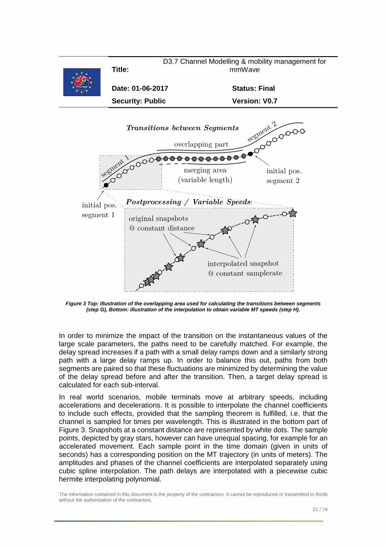

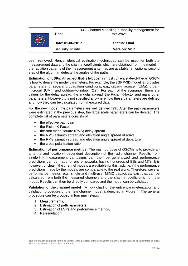
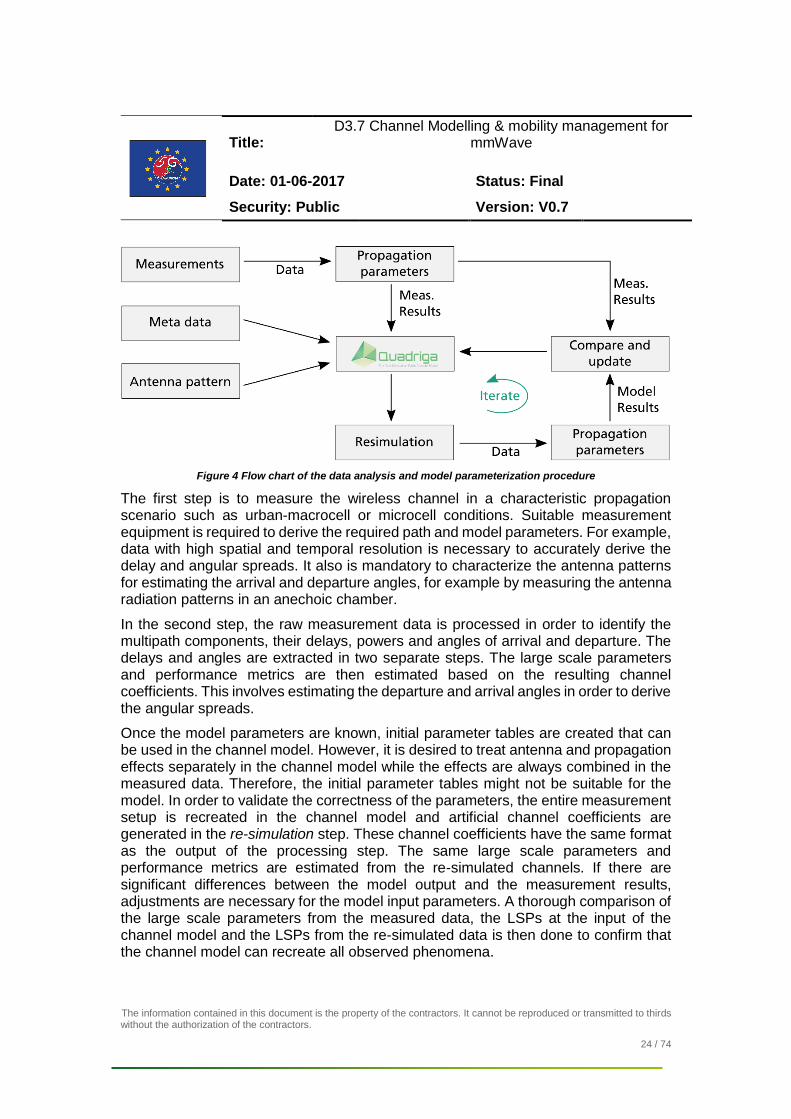
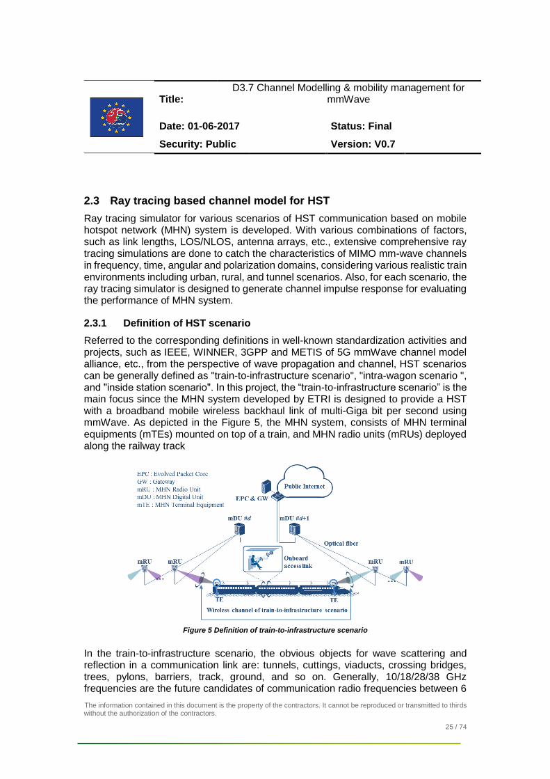

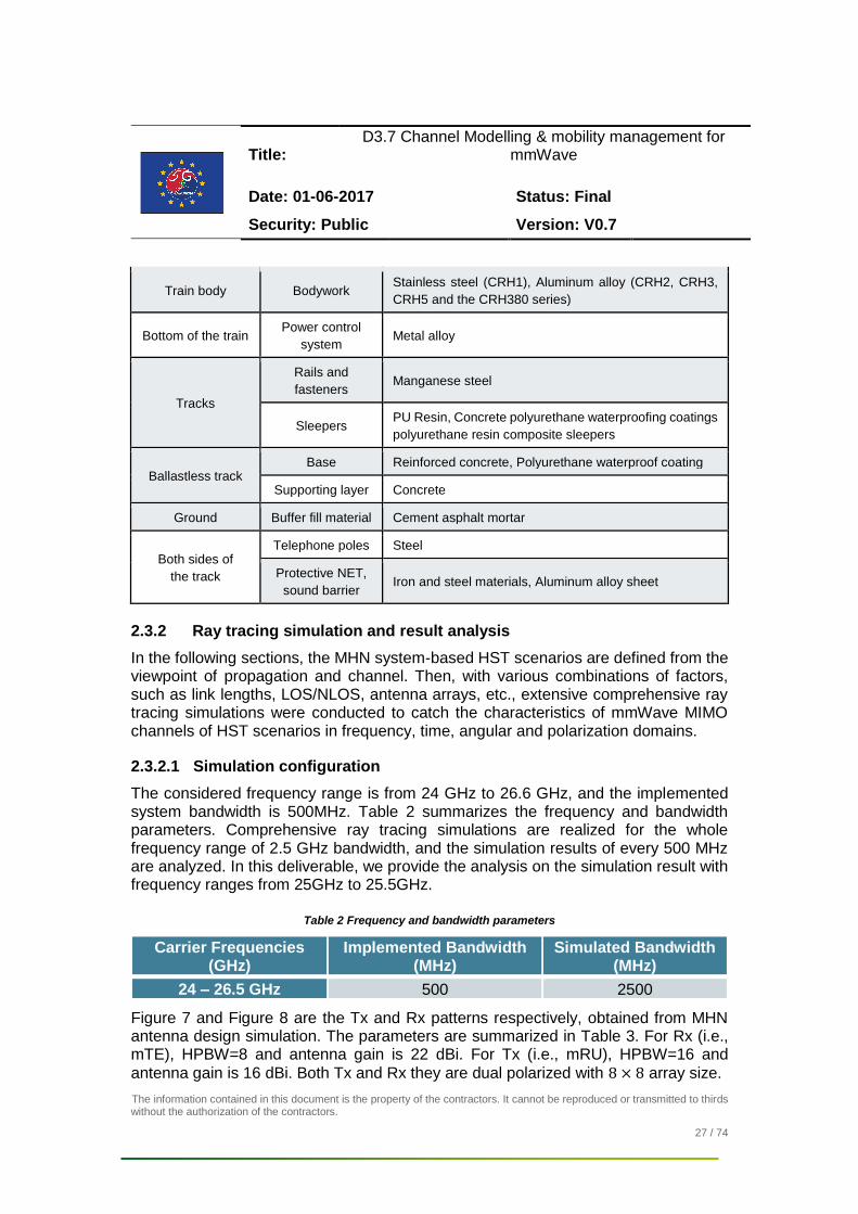
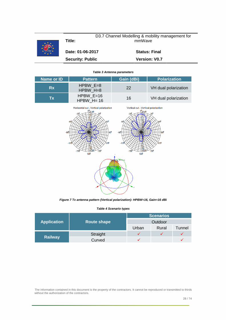
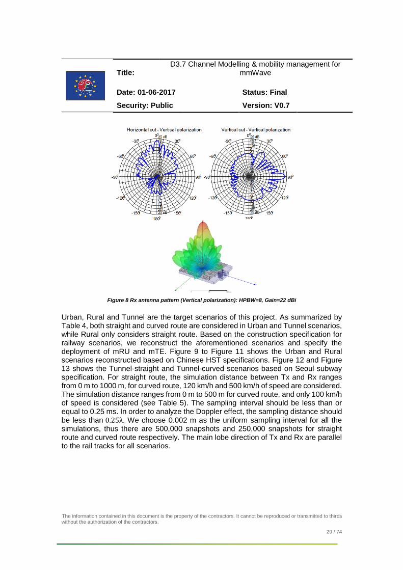
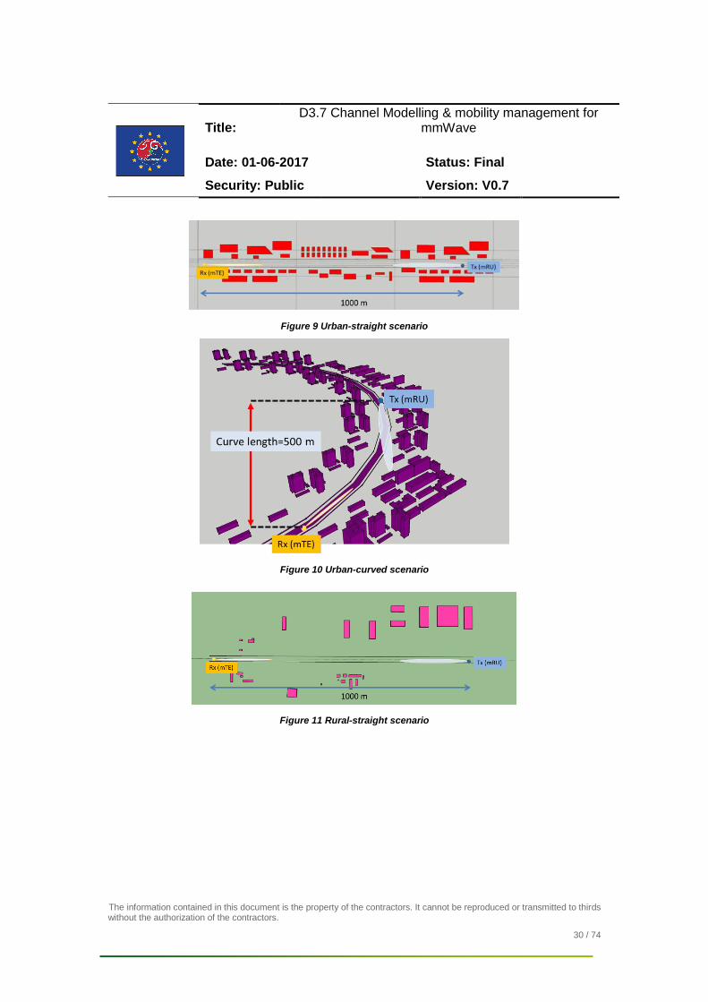

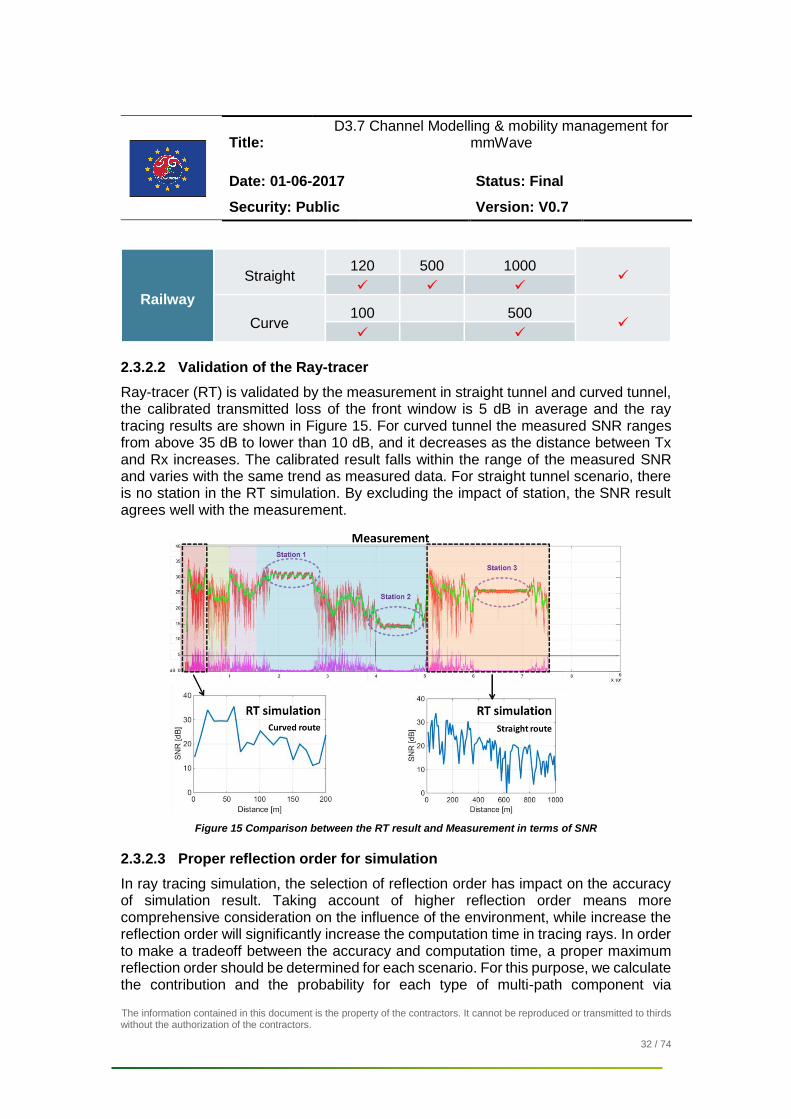


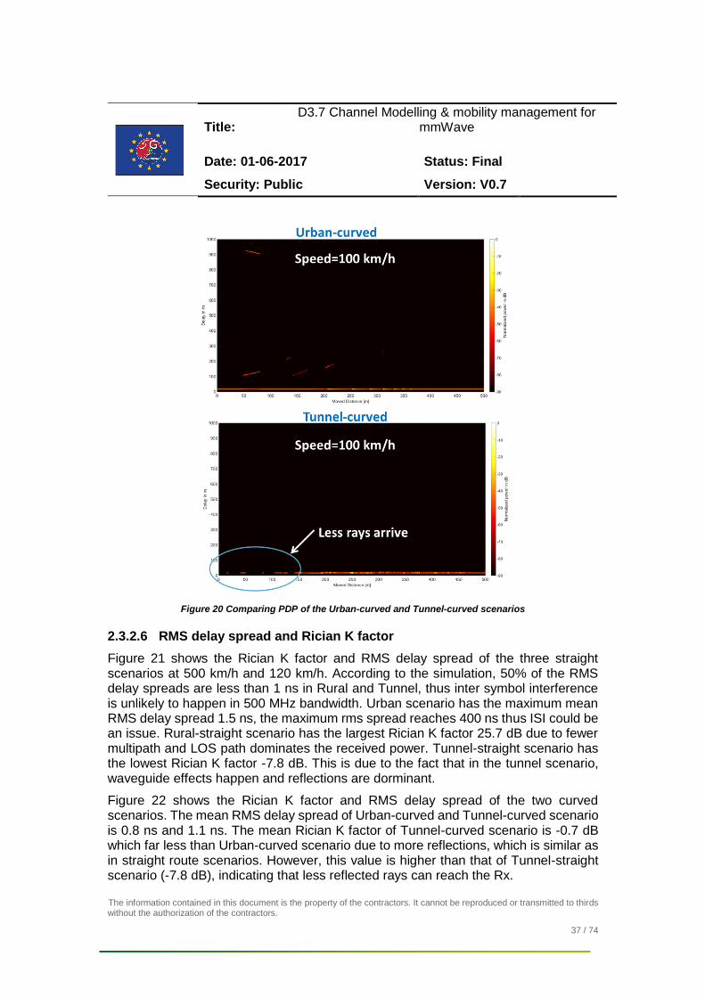
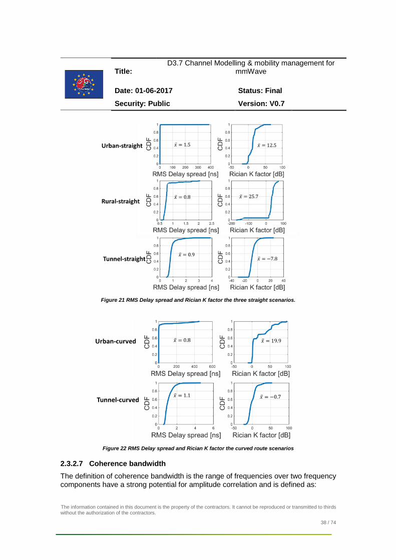


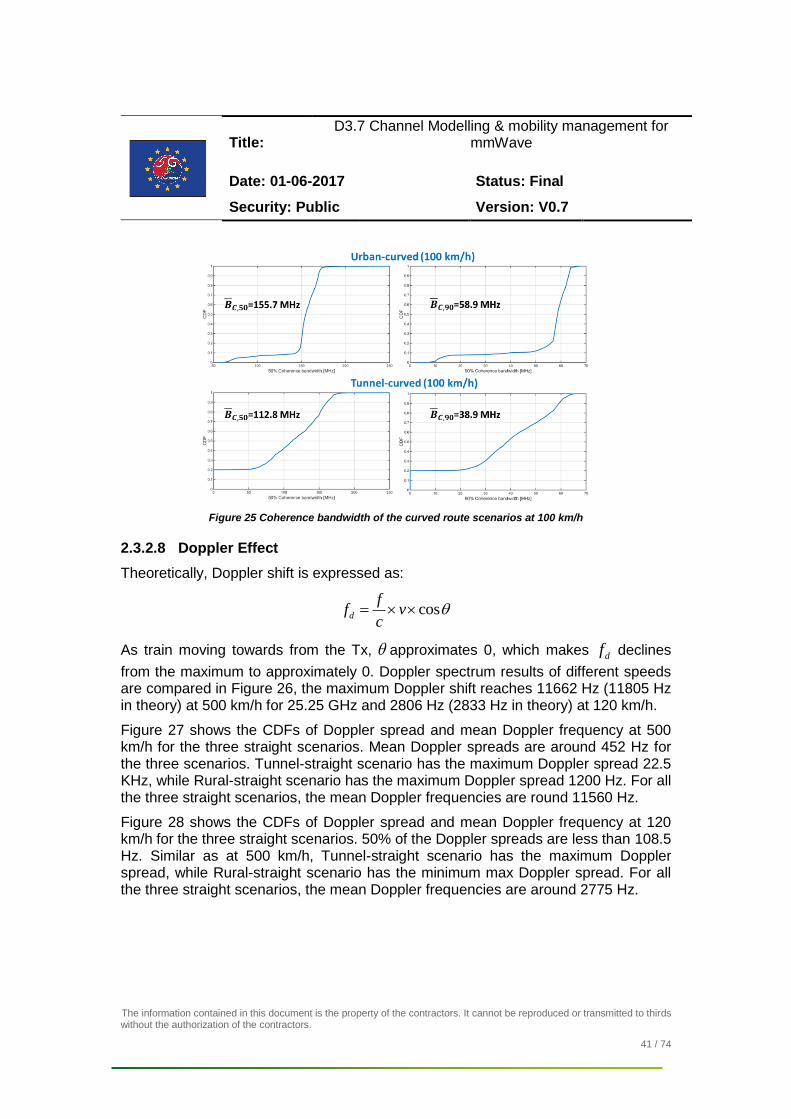
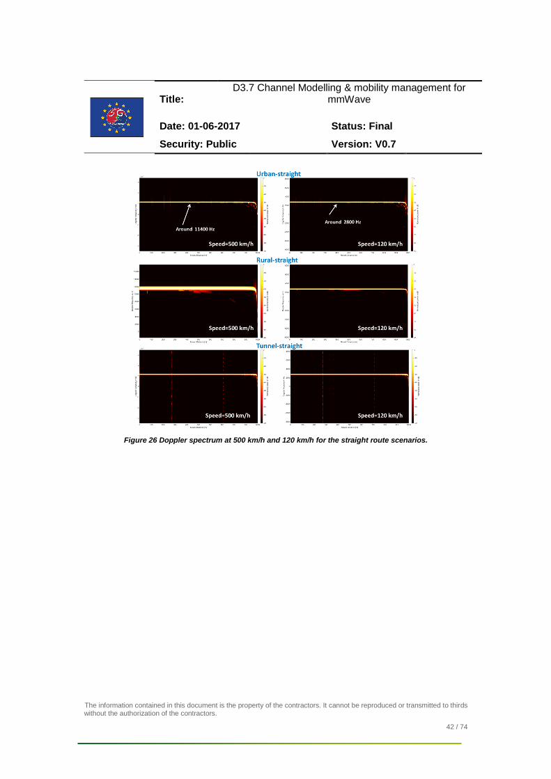
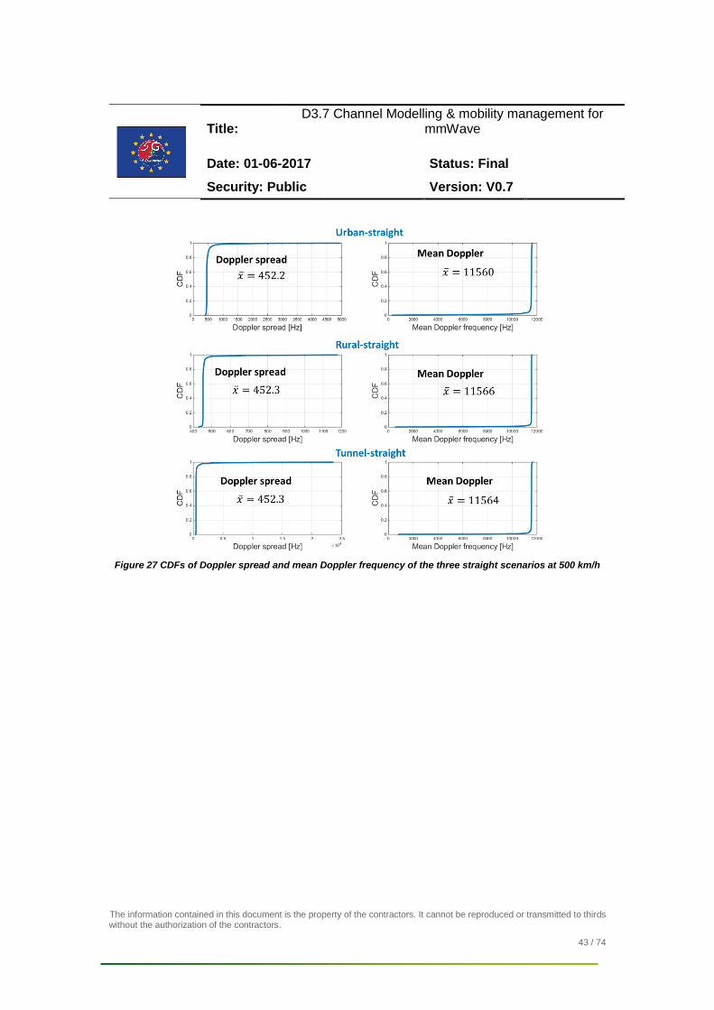
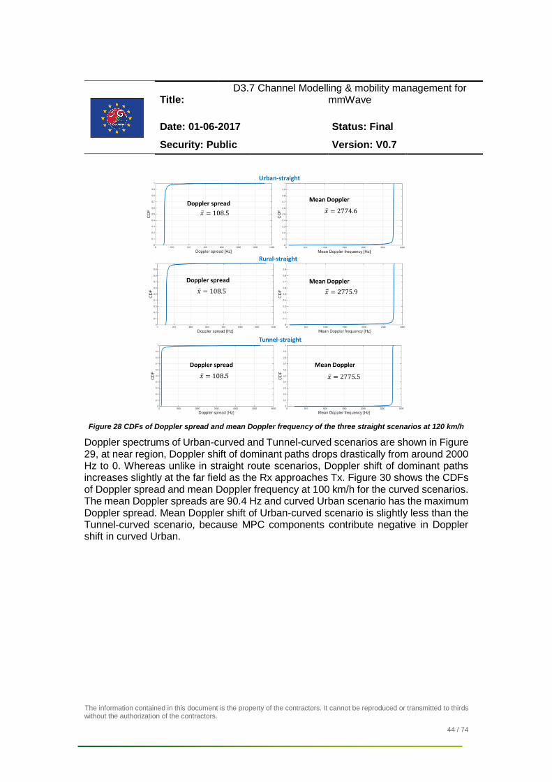

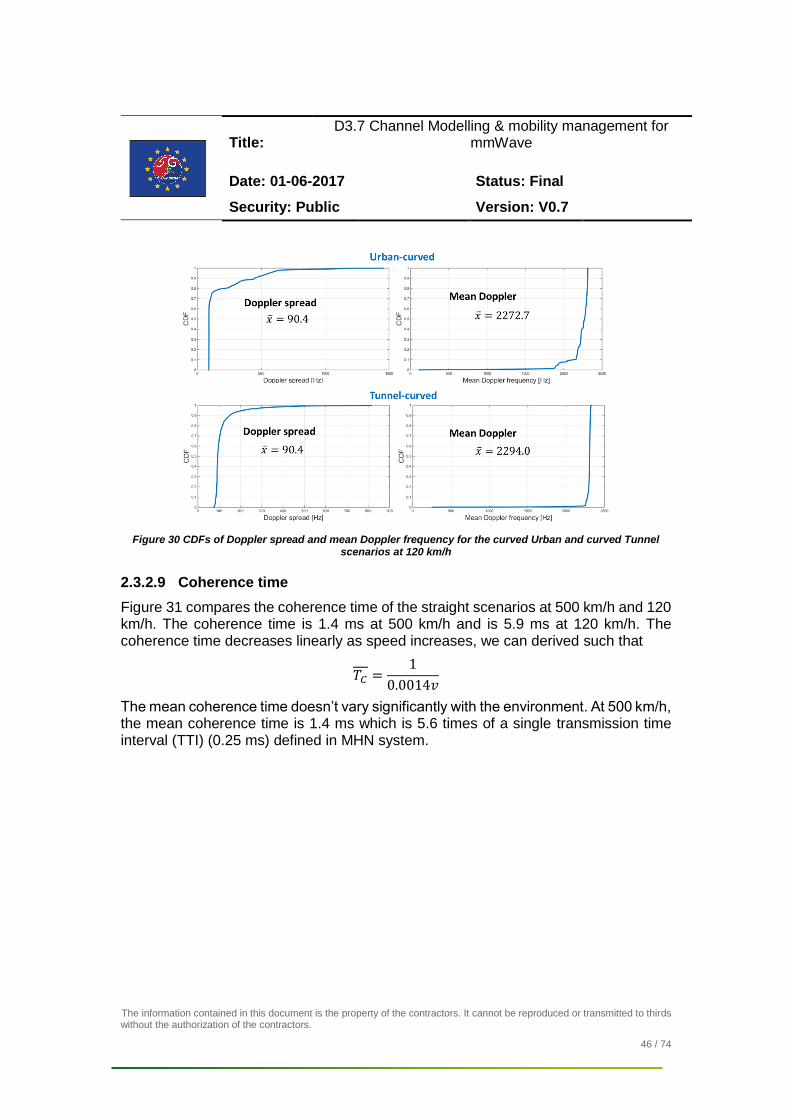
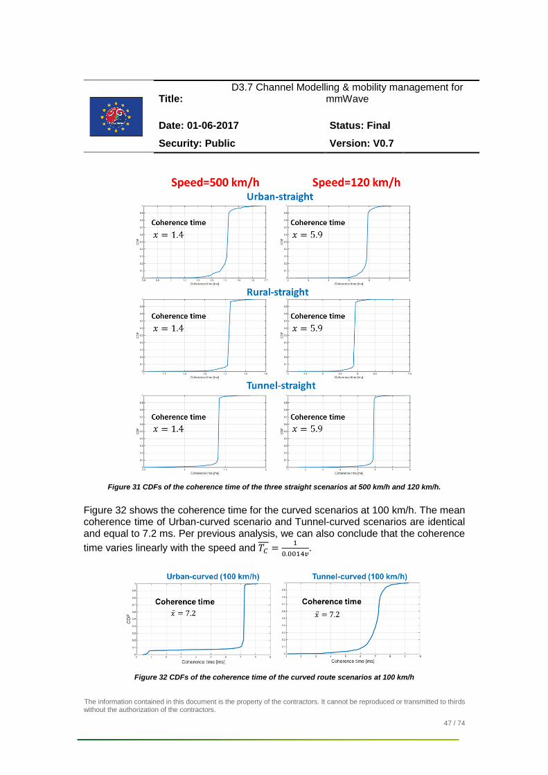

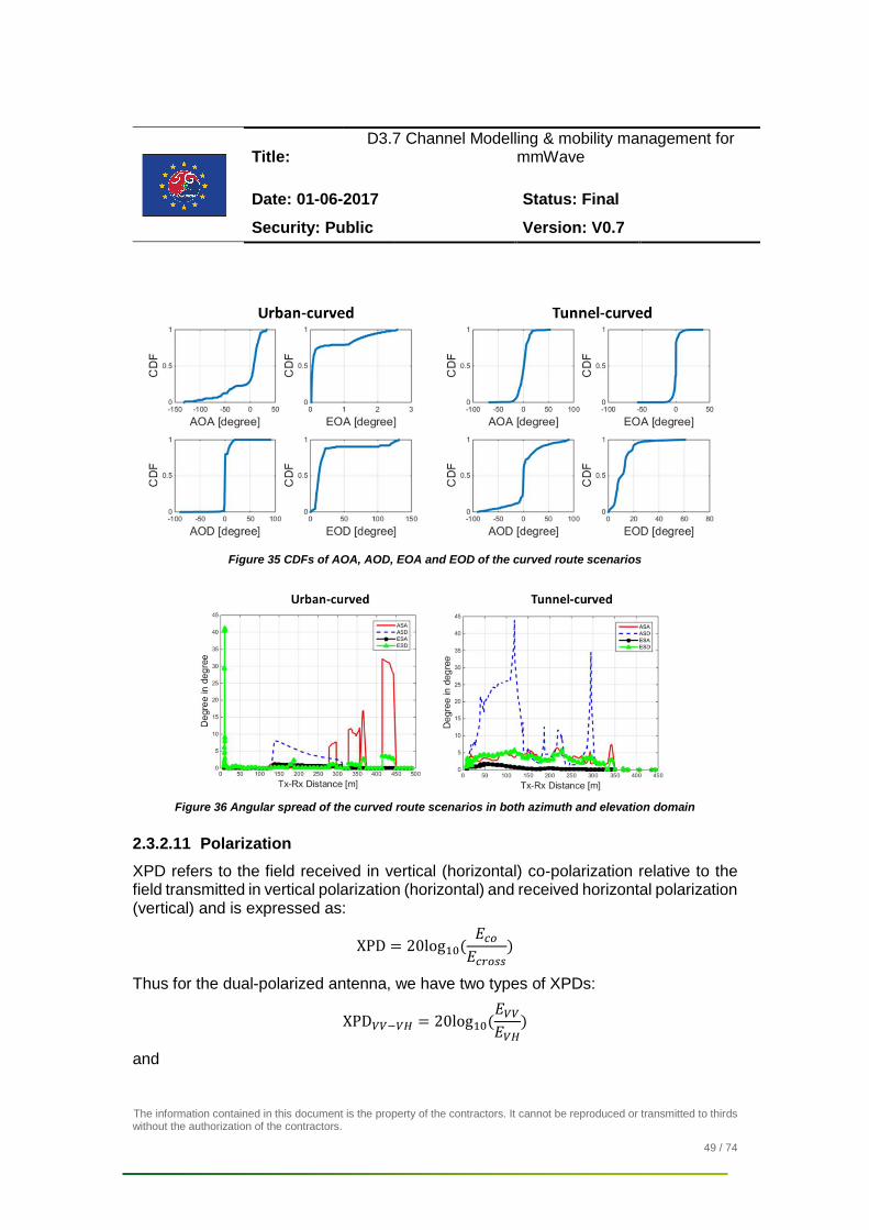

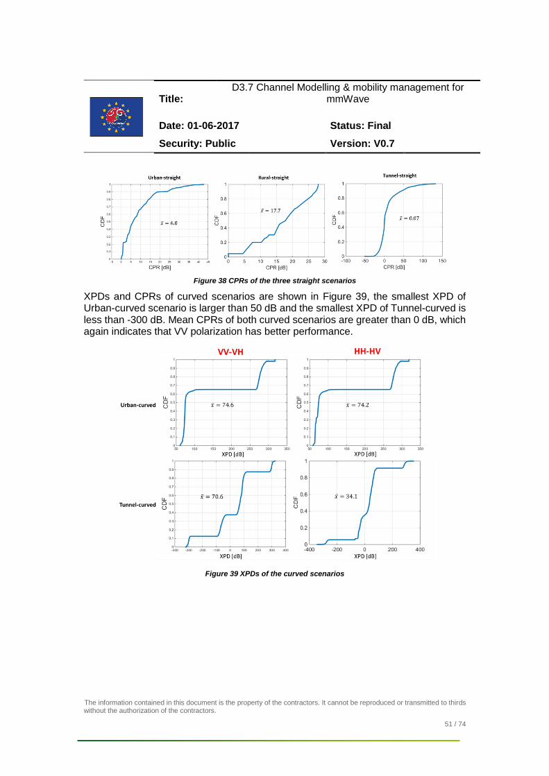
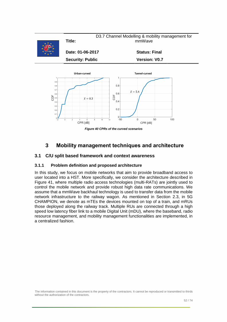
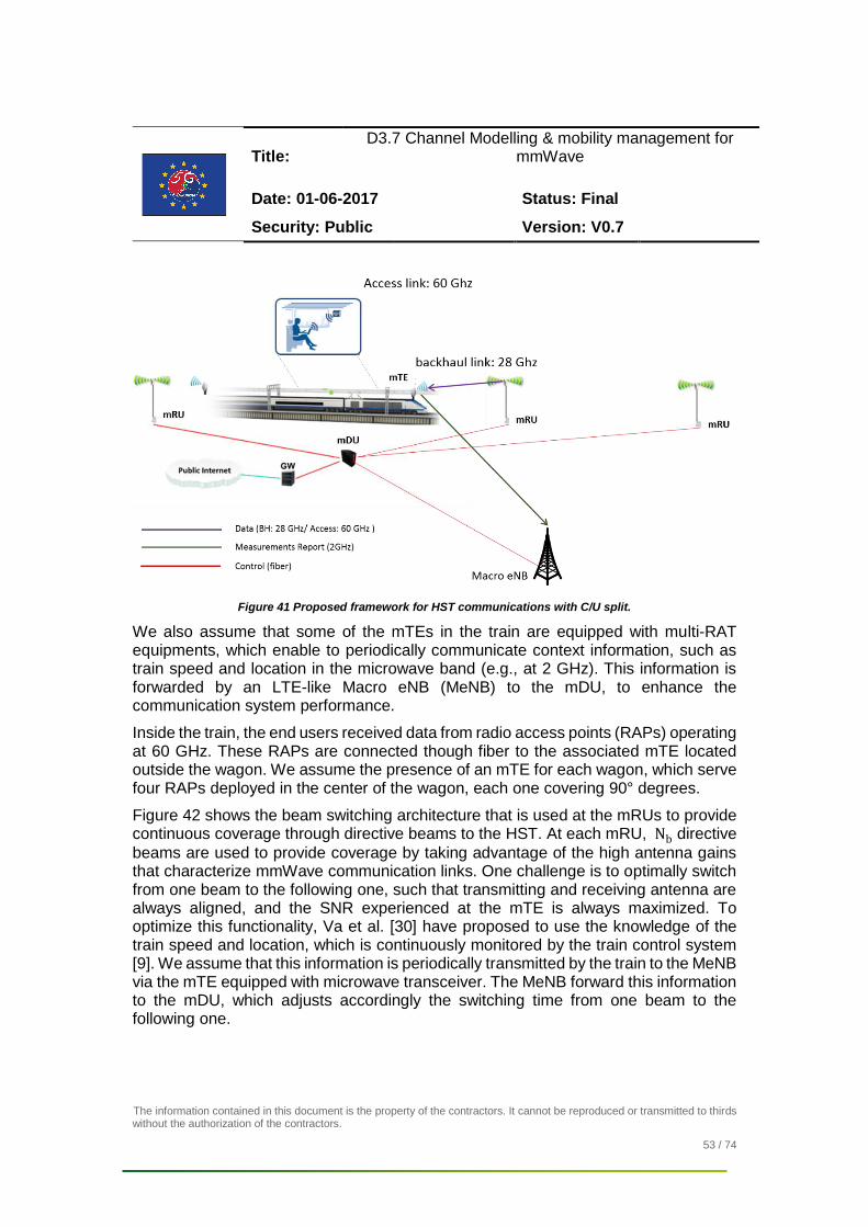
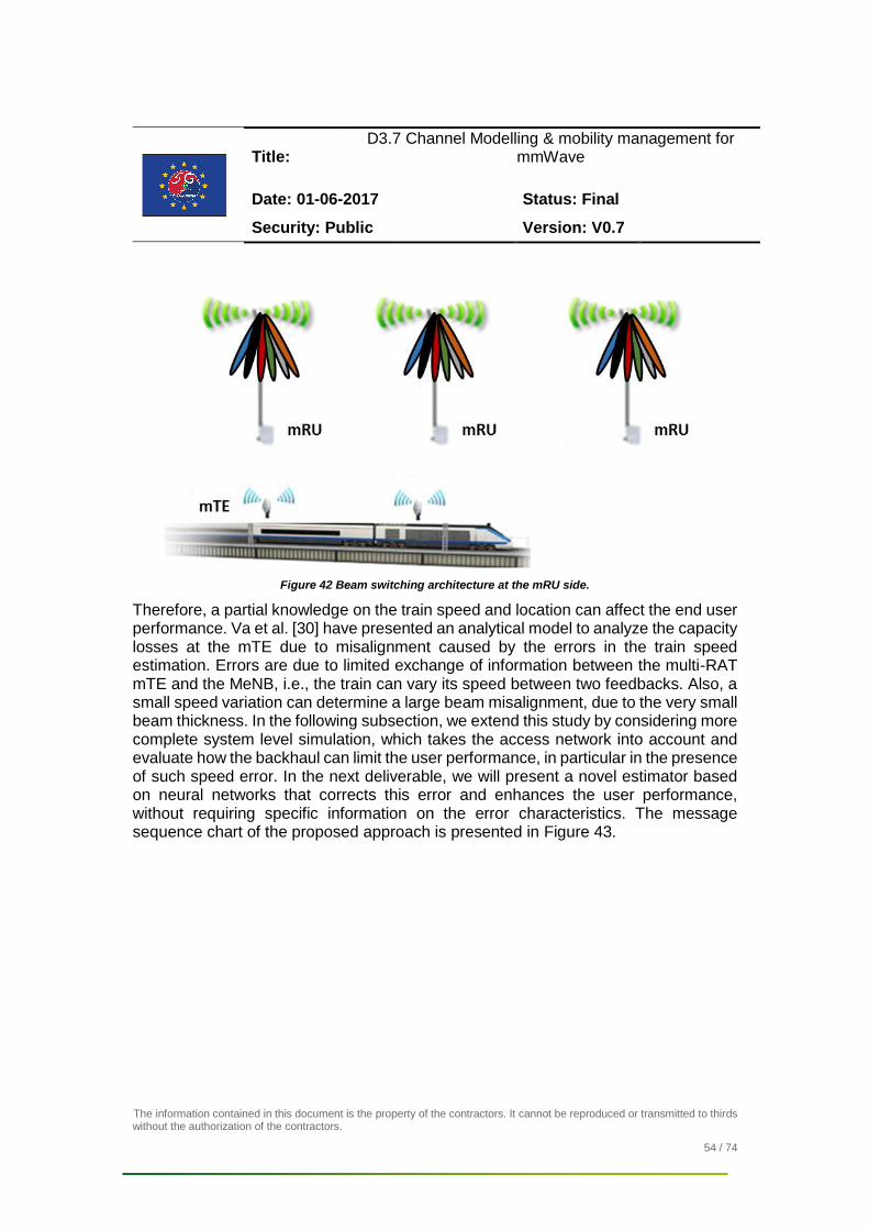
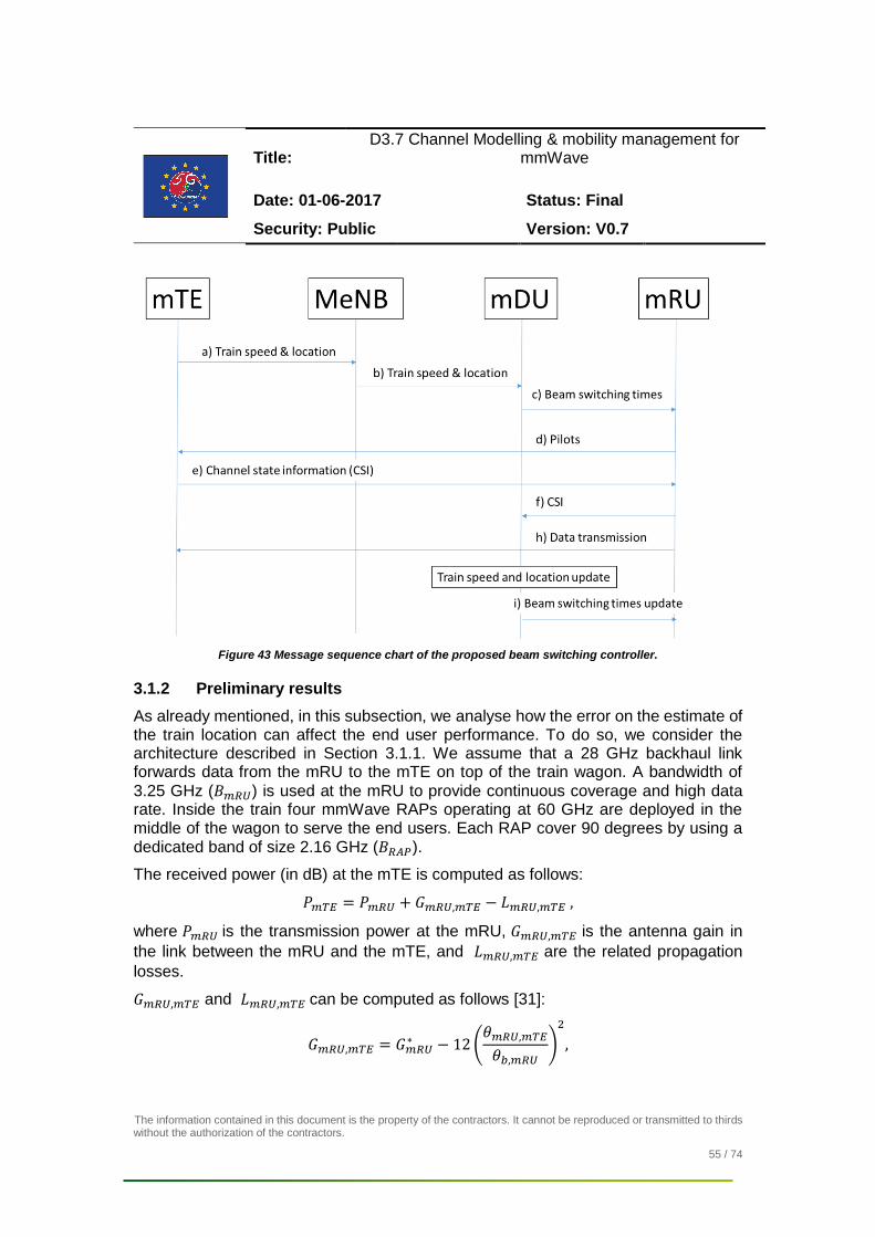
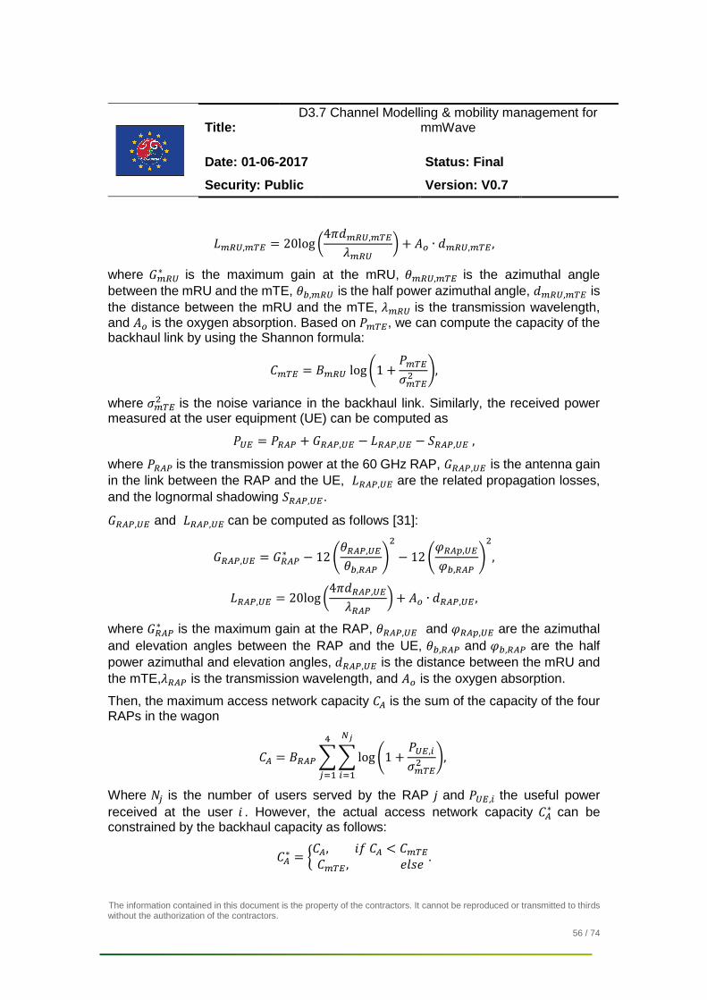

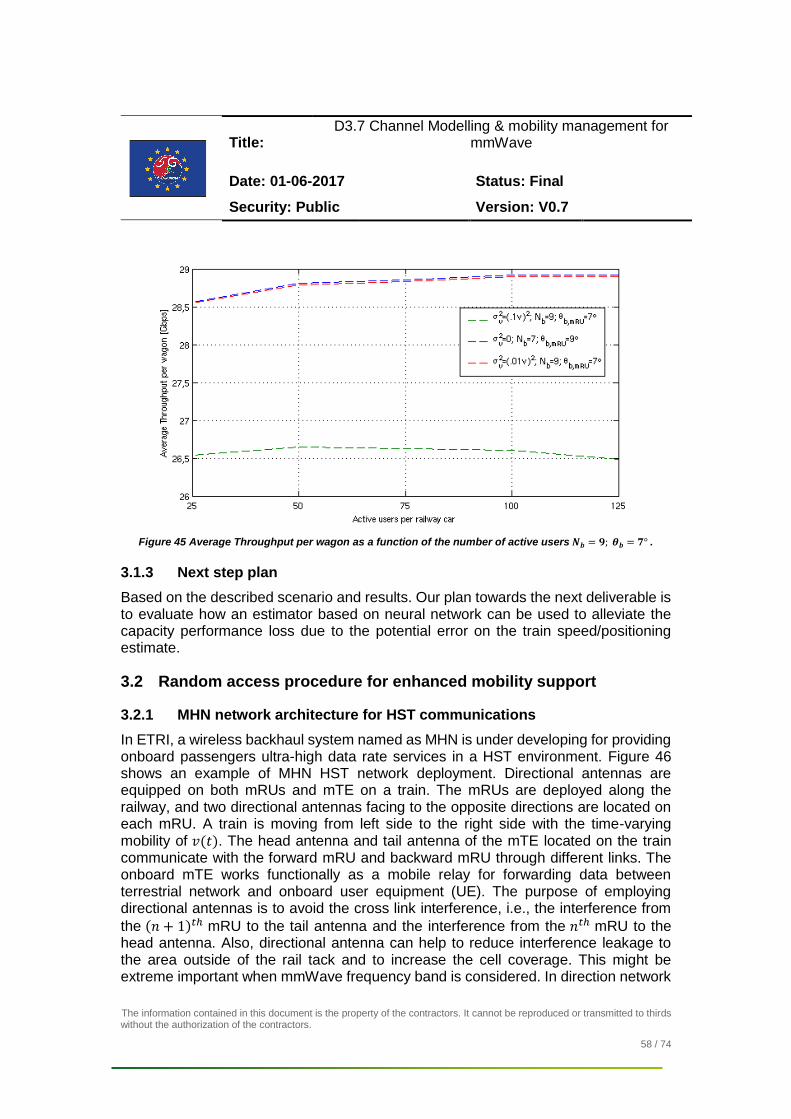


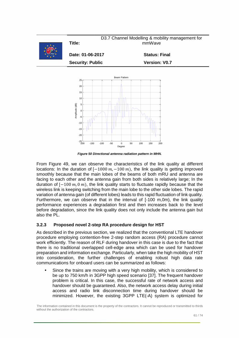


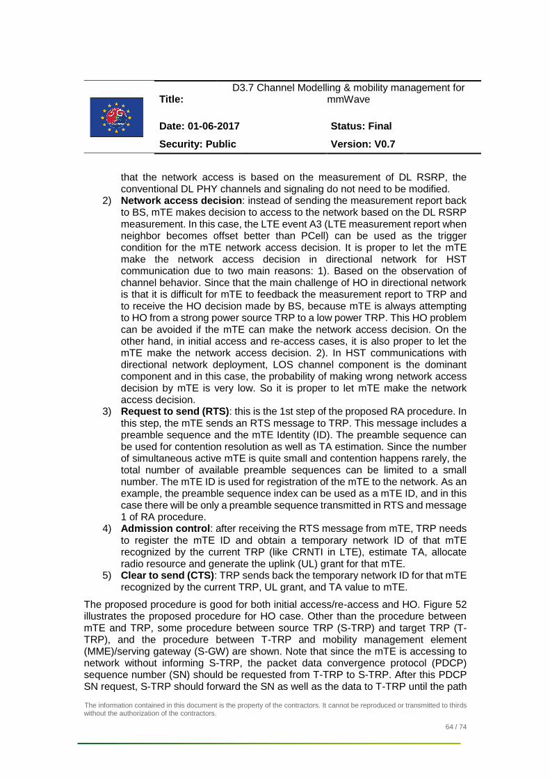
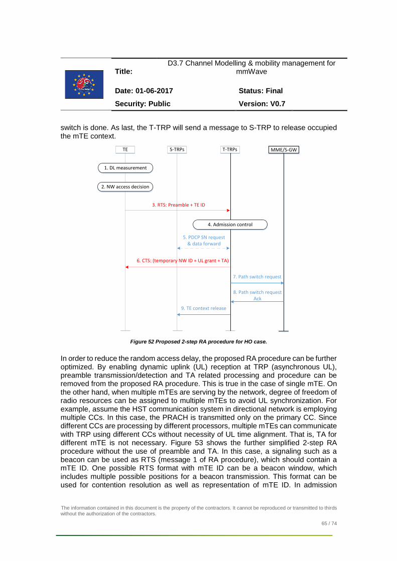
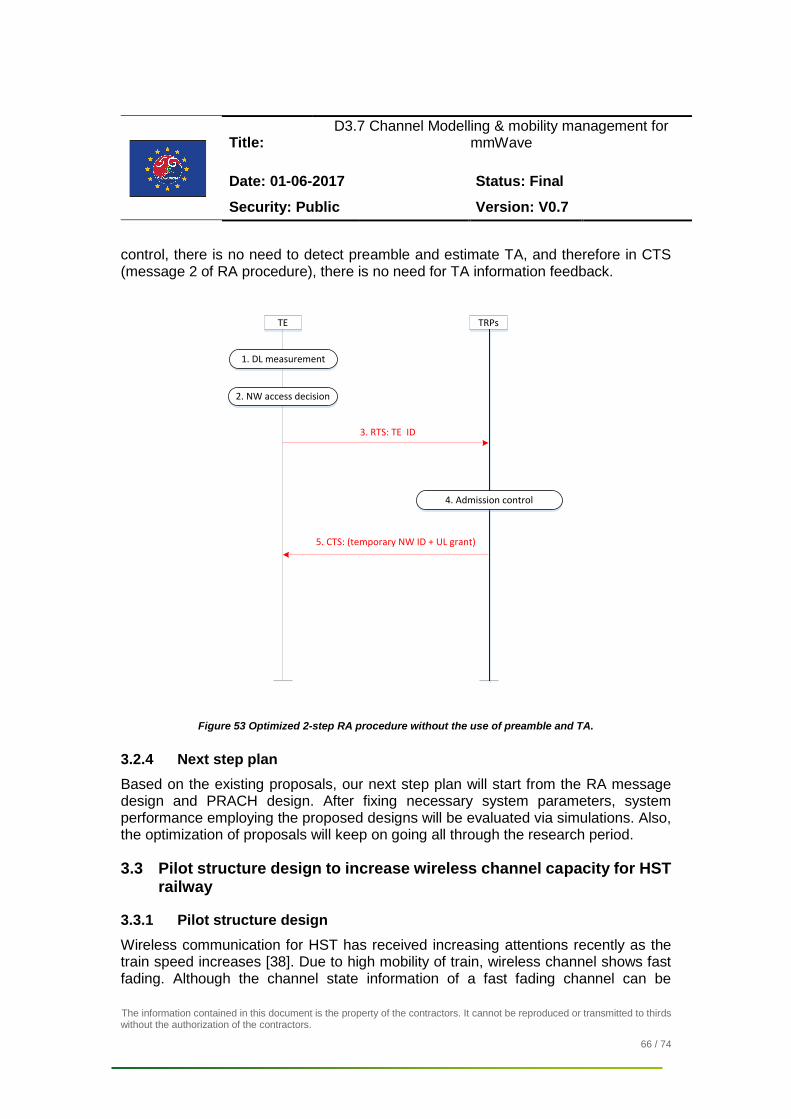
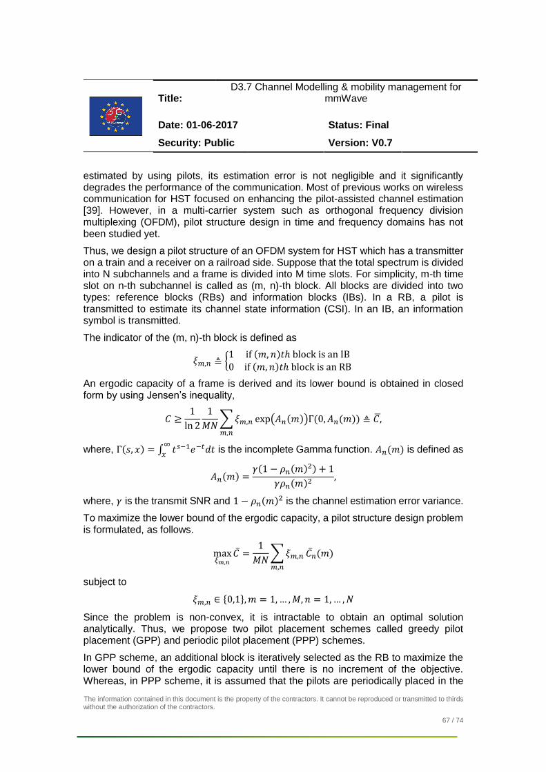
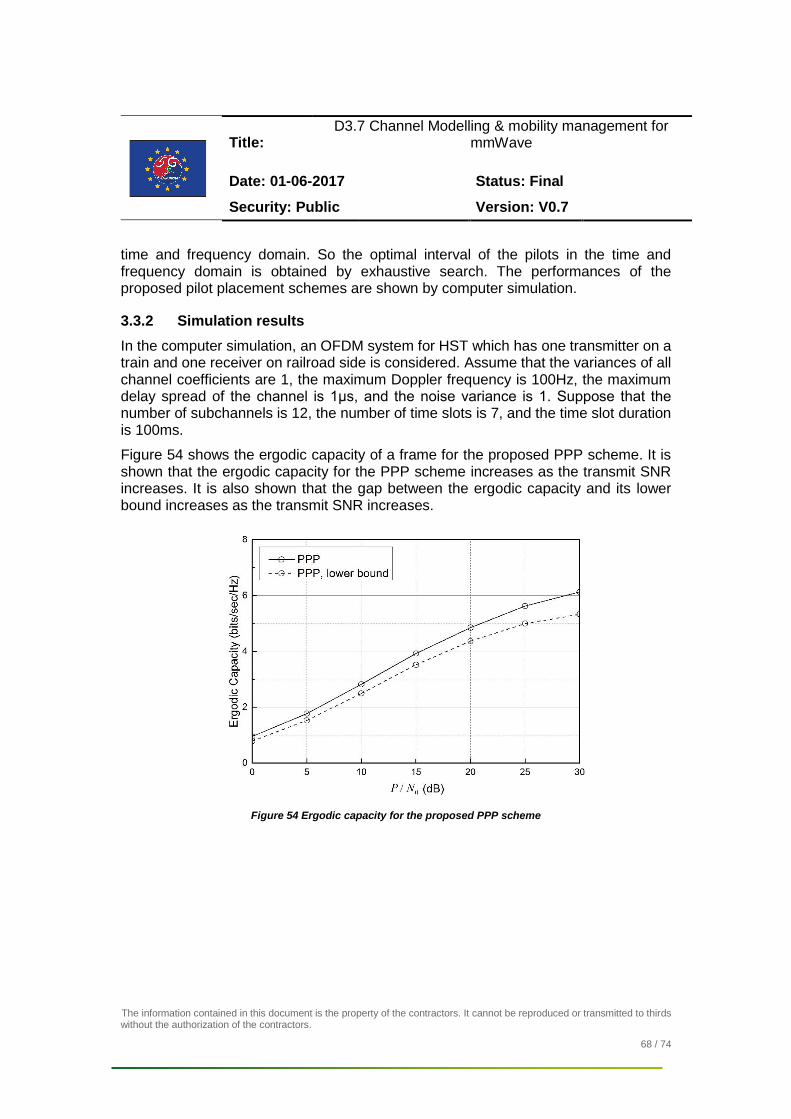
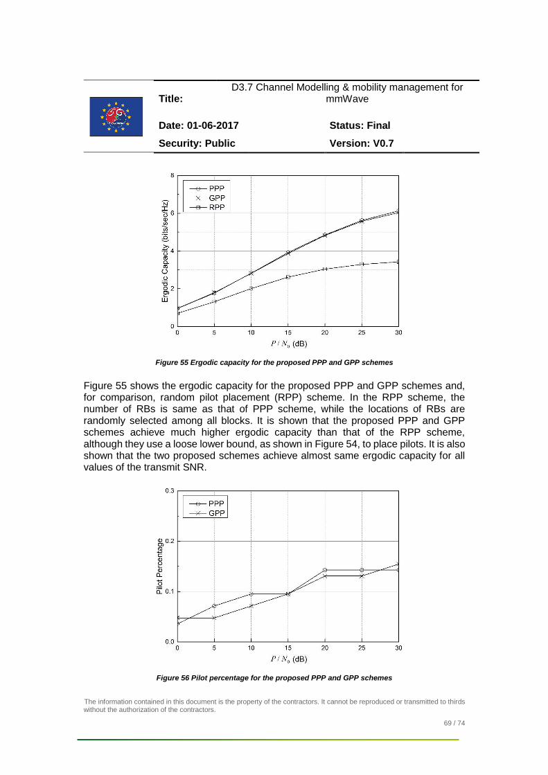


![D3.7: Proposal for an ethical framework for human …...D3.7: Proposal for an ethical framework for human enhancement [WP3 – Human Enhancement] Lead contributors Michael Kühler,](https://static.documents.pub/doc/80x56/60e47217d7cf2c579f492a00/d37-proposal-for-an-ethical-framework-for-human-d37-proposal-for-an-ethical.jpg)


