Deliverable D400€¦ · This project is co-funded by the European Union Deliverable D400.4 Impact...

www.eco-fev.eu

This project is co-funded

by the European Union

Deliverable D400.4

Impact assessment

version 19

dissemination Internal (then PU)

due date 15 May 2015

version date 08 June 2015

Impact assessment version 19

version date: 08 June 2015 ii

Contributions by

Authors

Bruno DALLA CHIARA (resp.)

Francesco DEFLORIO

POLITO

POLITO

Luca CASTELLO POLITO

Marco DIANA

Ivano PINNA

POLITO

POLITO

Miriam PIRRA

Camilla AUXILIA

POLITO

BLUETHINK

Valeria CANTELLO ENERGRID

Nadim EL SAYED TUB

Catrin GOTSCHOL FACIT

Luca BELLINO TECNOSITAF/MOBI-SERVICE

Maria Paola BIANCONI

Paolo BARGERO

CRF

BLUETHINK

Paolo GUGLIEMI POLITO

Fikret SIVRIKAYA TUB

Jean Christophe MAISONOBE CG38

Witold KLAUDEL REN


version date: 08 June 2015 iii

Revision and history chart

Version Date Comment

1 30.10.2014 Initial template

2 10.11.2014 First draft

3 01.12.2014 Comments and revisions from BLU plus updates

3R 02.12.2014 Text updates and assignment of specific sections to partners

4 08.12.2014 Extended version of the draft for ENERGRID

5 18.12.2014 Extended version of the draft for all and for POLITO and FACIT

6 21.01.2015 Updated v. by ENERGRID (business model) and POLITO (simulat. CWD)

7 02.02.2015 More details on CWD simulation and business plan (ENERGRID, POLITO)

8 03.04.2105 Updates by POLITO (MD) and FACIT (CG)

9-15 4-30.04.2015 Final contributions (POLITO; TUB), editing; ready for review

16-17 4.5.2015 Revision and comments by the two reviewers

18

19

20

14.5.2015

26.05.2015

08.06.2015

Final version after internal review

Amendments after programme officers’ review and comments on

the 25.5.2015

Final version

Project funding

7th Framework Programme

GC-ICT-2011.6.8: ICT for fully electric vehicles

Specific Targeted Research Project (STREP)

Grant Agreement No. 314411

Contact information

Coordinator

Dr. Massimiliano Lenardi

Hitachi Europe Limited

955 route des Lucioles “Ecolucioles B2”

06560 Valbonne Sophia-Antipolis France

phone: +33 (0)4 89 87 41 00

e-mail: [email protected]


version date: 08 June 2015 iv

Table of contents

Executive Summary 12

1. Introduction 13

2. Impact assessment of charging technologies 17

2.1. Impact assessment in parking areas for wired charging 18

2.1.1. Transport and traffic issues 18

2.1.2. Forecasts and energy issues relate to marker forecasts 19

2.2. Impact assessment of CWD on selected traffic flow scenarios 25

2.3. Impact assessment of CWD on motorways 26

2.3.1. CWD Business Model for Motorway Concessionaires 27

2.3.2. Simulation model for the EVSE management and scenario description 34

2.3.3. Main results of simulated scenarios 53

2.3.4. Use of scenario results for business model 63

2.3.5. Experimental results in a ring road scenario 65

2.3.6. Use of the simulation model for impact assessment of CWD on the power grid 69

2.4. Impact assessment of CWD in urban arterials 72

2.4.1. Data collection and modelling 73

2.4.2. Traffic flow calibration and model validation 75

2.4.3. Scenario explored 76

2.4.4. The CWD performance estimation 78

3. Impact assessment concerning service quality adopting performance

indicators 82

3.1. Key Performance Indicators 82

3.2. Evaluation of charging infrastructure 84

3.2.1. Interfaces and technologies of the architecture of the charging infrastructure system 85


version date: 08 June 2015 v

3.2.2. Technology impact assessment 88

3.3. Test site realisation in Grenoble 93

3.4. Installation and evaluation of inductive charging 97

3.4.1. Test site: installation and first trials at the test site in Italy 97

3.4.3. Scope of the evaluation 105

3.4.4. Description 105

3.4.5. Results 106

4. Impact assessment on mobility: general viewpoint and users 115

4.1. Mobility in a shared vision for FEV 115

4.1.1. New mobility paradigms: car sharing 115

4.1.2. Car pooling 119

4.1.3. Possible conflicts 120

4.1.4. Sharing economy trend 120

4.2. Economic viewpoint for the user 123

5. Demand analysis 126

5.1. Introduction 126

5.2. Expected sales evolution 127

5.3. Profiles of users, potential users and not users 129

5.4. Trip purposes and driving distances 133

5.5. Attitudes related to EV, especially before and after its use 134

5.6. Capital costs vs. operating costs and related subsidies 136

5.7. Concluding remarks and lessons learned for the take-up of eCo-FEV

technologies 139

6. Energy and environmental impact assessment 142

6.1. Overall energy assessment 142


version date: 08 June 2015 vi

6.1.1. Well-to-wheel index definition 142

6.1.2. WTW key points 143

6.1.3. Different types of EVs 144

6.1.4. WTW applied to EVs 146

6.1.5. WTW applied to fuel combustion vehicles 148

6.1.6. WTW calculation results 150

6.1.7. Conversion from gCO2 to Euro 152

7. Conclusions 156

8. References 158

8.1. General references 158

8.2. References for chapter 5 159

9. Annex 1 – Energy scenarios 162


version date: 08 June 2015 vii

List of Figures

Figure 1. Main reasons at the basis of WP 400 ......................................................... 14

Figure 2. Extract from EU White paper ................................................................. 14

Figure 3. Distribution of traffic flows by time of the day and days of the week. UK, 2013 ..... 29

Figure 4. EU27 Electric Vehicle Registrations in 2020 and 2030 ..................................... 30

Figure 5. Price of Electricity (pre-tax) by sector ...................................................... 31

Figure 6. Cost Components of Average Electricity Price ............................................. 32

Figure 7 .Scenario layout for CWD in a road with three lanes ....................................... 35

Figure 8 Scenarios explored for the electrical light-van in EMPTY CONDITIONS (2500 kg) ...... 38

Figure 9. Scenarios explored for the electrical light-van in FULL LOADED CONDITIONS (3500 kg)

............................................................................................................... 39

Figure 10. Influence of speed and LCD on the ∆SOC for an electrical city car for the adopted

EVSE settings, after 1 km ................................................................................. 41

Figure 11. Positive and negative energy for the empty electrical light-van (2500 kg) after 20

km in the charging lane, at different speeds for the selected CWD layout (LCZ= 20m, I=30m) 43

Figure 12. Several trajectories in the time-space diagram to trace the arrival times of different

vehicle types at consecutive nodes. .................................................................... 45

Figure 13. Example of a cooperative use case scenario for CWD applications [source:

elaboration on ETSI, 2011] ............................................................................... 46

Figure 14.The cases of single and multiple overtaking manoeuvres ................................ 49

Figure 15. Examples of vehicle SOC [kWh] along the CWD lane for five vehicles with different

starting status .............................................................................................. 51

Figure 16. Traffic of FEVs on CWD charging lane during the day at entrance section (node 0)

end exit section (node 20) in Reference scenario (REF) .............................................. 55


end exit section (node 20) in HTL scenario ............................................................ 56


end exit section (node 20) in LFT Scenario............................................................. 56


end exit section (node 20) Alternative scenario (ALT) ............................................... 57

Figure 20. Turin ring road with main secondary accesses ............................................ 65

Figure 21. Space-time relationship for "in" vehicles in scenario 1 .................................. 67

Figure 22. Space-time relationship for "in" vehicles in scenario 2 .................................. 67

Figure 23. Real and simulation environments of the urban arterial in Turin (Italy) .............. 74


version date: 08 June 2015 viii

Figure 24. Traffic control regulation at one simulation node ....................................... 75

Figure 25. Maximum stop time [s] for each FEV ....................................................... 79

Figure 26. Global charging time [s] for each FEV ..................................................... 80

Figure 27. Energy gains for FEV along the arterial .................................................... 81

Figure 28. Charging infrastructure System ............................................................. 86

Figure 29. Technologies of the Charging Infrastructure .............................................. 88

Figure 30. Test site area .................................................................................. 97

Figure 31. Static wireless recharging zone ............................................................. 98

Figure 32. Excavations .................................................................................... 98

Figure 33. Shelter .......................................................................................... 99

Figure 34. Area for the wireless recharging in motion ................................................ 99

Figure 35. ANPR .......................................................................................... 100

Figure 36. Exhisting builing ............................................................................. 100

Figure 37. Power Transformer ......................................................................... 101

Figure 38. Power Room ................................................................................. 101

Figure 39. Control room ................................................................................ 102

Figure 40. Work location ................................................................................ 102

Figure 41. Plug in ........................................................................................ 103

Figure 42. Prototypal structure for the laboratory test of the IPT CWD system (Politecnico di

Torino, energy area Laboratory, April 2015) ......................................................... 106

Figure 43. Efficiency calculation scheme ............................................................. 107

Figure 44. Turn ON of a transmitting coil with the presence of the vehicle ..................... 107

Figure 45. Turn OFF of a transmitting coil ........................................................... 108

Figure 46. Horizontal misalignment test.............................................................. 110

Figure 47. Vertical misalignment test ................................................................ 110

Figure 48. Procedure for vehicle identification through the DC/HF converter .................. 112

Figure 49. Measurement of the magnetic field induction during the operation of the system, at

the Energy Laboratory (Politecnico di Torino, Dept.DENERG) ..................................... 114

Figure 50. Expectations about the percentage of increase of electric car sales in the next 10

years (taken from Thiel et al. (2012)) ................................................................ 127

Figure 51. EV Market: Sales Estimates, Global, 2012–2018 (taken from Frost (2014)). ........ 129

Figure 52. EV Charging Infrastructure Marke t: Sales Estimates for Inductive Charging Stations

by Charging Capacity, Global, 2012–2020 (taken from Frost (2014)). ............................ 129


version date: 08 June 2015 ix

Figure 53. Probability of purchasing an electric car with its current average characteristics by

socioeconomic segment (taken from Thiel et al. (2012)). ......................................... 131

Figure 54. Degree of importance of factors that influenced the choice of an EV as perceived by

EV owners in Norway in 2014 (taken from Figenbaum et al. (2013)). ............................ 133

Figure 55. Level of agreement in percent to the questionnaire items. (taken from Bunce et al.

(2014)). ................................................................................................... 135

Figure 56: Cost of EVs compared to traditional cars in Norway, Sweden and Denmark

(Haugneland, 2014) ...................................................................................... 138

Figure 57. Values used for calculating the payback period and total cost of the EV in its

lifetime (taken from Lopes et al. (2014)). ........................................................... 139

Figure 58. WTW total expected GHG emissions for fuel combustion vehicles ................... 149

Figure 59. WTW GHG-emissions of different xEV as function of GHG intensity of the utilized

electricity ................................................................................................. 150

Figure 60.WTW GHG Emissions for xEVs .............................................................. 151

Figure 61. EU ETS carbon spot price .................................................................. 153

Figure 62. Final Energy Consumption (Mtoe) and GHG Emissions by Sector ..................... 163

Figure 63. GHG Emissions by Transportation Modes ................................................ 163

Figure 64. Length and Type of Ten-T Roads.......................................................... 164

List of Tables

Table 1. Electric light van data .......................................................................... 38

Table 2. Electric city car data ........................................................................... 40

Table 3. Different FEVs scenarios ....................................................................... 54

Table 4. ALT scenario: traffic counting along the CWD lane ........................................ 58

Table 5. ALT scenario: average headway on the CWD lane .......................................... 58

Table 6. ALT scenario: traffic counting along the CWD lane during the peak hour period (15h-

18h) with 5 minutes resolution .......................................................................... 59

Table 7. ALT scenario: maximum delay for charging vehicles ....................................... 59

Table 8. ALT scenario: speed during the day for the OUT vehicles ................................. 60

Table 9. ALT scenario: effect of the CWD on the vehicles average SOC ........................... 60

Table 10. ALT scenario: effect of the CWD on the low-SOC vehicles ............................... 61

Table 11. Energy received by FEVs between nodes during the 24 hour of the day in the

Reference scenario ........................................................................................ 61


version date: 08 June 2015 x

Table 12. Energy received by FEVs between nodes during the 24 hour of the day in the HTL

Scenario ..................................................................................................... 62

Table 13. Energy received by FEVs between nodes during the 24 hour of the day in the LFT

scenario ..................................................................................................... 62

Table 14. Energy received by FEVs between nodes during the 24 hour of the day in the

Alternative scenario ....................................................................................... 63

Table 15. Average SOC [kWh] of "in" vehicles, node by node, with a 1 min time resolution, for

scenario 1 ................................................................................................... 68

Table 16. Average SOC [kWh] of "in" vehicles, node by node, with a 1 min time resolution, for

scenario 2 ................................................................................................... 68

Table 17. Crossing flow (east-west) for each vehicle type ........................................... 76

Table 18. Crossing flow (west-east) for each vehicle type ........................................... 77

Table 19. Travel time (East-West) for each vehicle type ............................................ 77

Table 20. Travel time (West-East) for each vehicle type ............................................ 78

Table 21. List of performance metrics for eCo-FEV service quality assessment .................. 84

Table 22- Electricity pathways as indication for GHG intensity from electricity ............... 146

Table 23. WTW total expected GHG emissions for fuel combustion vehicles ................... 149

Table 24. Carbon prices around the world ........................................................... 154


version date: 08 June 2015 xi

List of Abbreviations

C/S Charging Station

C/S CU Charging Station Control Unit

CI Charging Infrastructure

CWD Charge While Drive

CZ Charging Zone

DENM Decentralised Environmental Notification Message

EV Electric Vehicle

EVSE Electric Vehicle Supply Equipment

FEV Fully Electric Vehicle

GDP Gross Domestic Product

HMI Human Machine Interface

ICE Internal Combustion Engine

ITS Intelligent Transport Systems

OBU On-Board Unit

POI Point of Interest

POTI Position and Time Information

RADIUS Remote Authentication Dial-In User Service

RSU Road Side Unit

SNMP Simple Network Management Protocol

SoC State of Charge (Battery)

SoH State of Health (Battery)

VDP Vehicle Data Provider

VRM Vehicle Relationship Message

WPT Wireless Power Transfer

version date: 08 June 2015 12

Executive Summary

The eCo-FEV project aims at achieving a breakthrough in Fully Electric Vehicle (FEV)

introduction by proposing a general service platform for integration of FEVs with different

infrastructure systems cooperating with each other – thus allowing precise FEV telematics

services and charging management services, based on real time information.

The general concept of eCo-FEV is based on the development of an innovative next generation

e-mobility infrastructure by mutual system cooperation among FEV and independent FEV-

related infrastructures being networked. The cooperative e-mobility infrastructure enables

information exchange between independent infrastructure systems in order to provide

efficient telematics and ITS services to FEV users. For this purpose, an eCo-FEV system is

defined and being developed by the consortium, which includes subsystems integrated at FEV,

at road side, at charging infrastructure and at backend to realise FEV assistance services

before and during a trip and charging.

The objective of this deliverable is to assess the impact of the whole eCo-FEV system. Based

on the use cases and requirements defined in WP200 and the WP300, it is related to demand

and supply matching having considered (WP410) the overall procedure for the verification and

validation of all systems being developed and integrated in WP300. The methodology defined

within WP410 has been applied throughout eCo-FEV tests in WP300 and WP430, for being

evaluated in WP440.

Given the twofold aim for the recharging system, to be useful both for wireless inductive

charging (CWD) and the conductive (wired, static) one, the impact assessment takes into

account also and in particular flexible infrastructures, both wired and wireless.


1. Introduction

WP400 aims at ensuring that the envisaged system is properly working (WP410-420-430) and at

assessing (WP440) whether it may have a positive impact on the transport system as a whole,

from the energy, environmental, motorised mobility viewpoints, including final user

perspective.

Particular emphasis is given to the definition and set up of the verification and validation plan,

measurement of the system performances, verification of the functionality, comparison with

different solutions, assessment of benefits, some quantification and characterisation of the

demand.

The main aims of all the WP400 are:

A. Definition and set up of the evaluation methodologies, including the verification and

validation plan;

B. Measurement of the system performances at the test sites;

C. Technical verification of the functionality of the system;

D. Comparison with different technological solutions;

E. Assessment of benefits of the eCo-FEV system in terms of overall energy consumption

and traffic flows;

F. Quantification and characterisation of the demand for FEVs related to the recharging

scenarios, by considering both the transport mode share and the market penetration.

The eCo-FEV system prototypes have been tested and evaluated, on the base of WP300

results within this project; yet this is out of the scope of this document being an aim of

D400.3.


The main basic reasons for the WP 400 are resumed in the following scheme.

Figure 1. Main reasons at the basis of WP 400

Figure 2. Extract from EU White paper


In particular, the WP 400 is structured as synthesised hereafter.

WP 400 - test and evaluation

• 410 - Evaluation methodology (M8 - M19, i.e. April 2013- March 2014)

• 420 - Test preparation and execution (M18 - M28, February 2013-December 2014)

• 430 - Technical evaluation (M21 - M31, May 2014-March/April 2015)

• 440 - Impact assessment (M21 - M31, as above)

As regards the Deliverable D400.1, “Evaluation Methodology, Test and Evaluation Plan”, it

was concluded on the 31st of January, with revision concluded by the 14th of March 2014.

We remember that the eCo-FEV project aims at achieving a breakthrough in FE) introduction

by proposing a general service platform for integration of FEVs with different infrastructure

systems cooperating with each other – thus allowing precise FEV telematics services and

charging management services based on real time information. The eCo-FEV system is defined

and being developed by the consortium, which includes subsystems integrated at FEV, at road

side, at charging infrastructure and at backend to realise FEV assistance services before and

during a trip and charging. The objective of the concluded deliverable D400.1 was then to

define the methodology for testing and verification of the whole eCo-FEV system and

functionality. Based on the use cases and requirements defined in WP200, it describes the

overall procedure for the verification and validation of all systems being developed and

integrated in WP300. The methodology defined here has been applied throughout eCo-FEV

tests in WP300 and WP400.

The verification has taken into account also, and in particular, flexible infrastructures, wired

and wireless, for both inductive and conductive recharging,.

As regards the Deliverable D400.2 "Evaluation Database Description", it was concluded by

the 28 February 2014, with revisions by the 25 April 2014.

As the first deliverable of this work package, D400.1 provided the testing and evaluation

guidelines for the technical verification and impact assessment of eCo-FEV systems and use

cases. The deliverable D400.2 complemented this by providing the dataset to be collected

during the tests for validation and evaluation purposes. Categorised by the high-level eCo-FEV

components of Backend, Transport Infrastructure, and On-Board Unit, the envisioned

evaluation datasets were presented in detail. Those are then visualised in the form of a


database schema that could be utilised for the implementation in the testing and evaluation

activities of the project (WP300, CRF). A generic data record template for logging the

experiments is also provided. The initial guidelines for test data collection in terms of the

required measurement frequency or the granularity of data are discussed wherever applicable.

The eCo-FEV system being developed throughout WP300 could be tested and evaluated in

WP400 (WP430), with two main objectives: on one hand, to ensure that the envisaged system

is properly working; on the other, to assess whether it may have a positive impact on the

transport system as a whole, from the energy, environmental, motorised mobility viewpoints,

including user acceptance.

The role of WP400 within the Impact assessment (resp. POLITO), through the WP440, can be

split as:

Consumption analysis

Charging and autonomy

Queuing problems

Parking areas

Charging network

Traffic analysis

Analysis of the demand

These goals will be reached through an evaluation that will cover the following aspects:

definition and set up of the evaluation methodologies, including the verification and

validation plan

measurement of the system performances at the test sites

technical verification of the functionality of the system

assessment of benefits of the eCo-FEV system in terms of overall energy consumption

and traffic flows

quantification and characterisation of the demand for FEVs related to the recharging

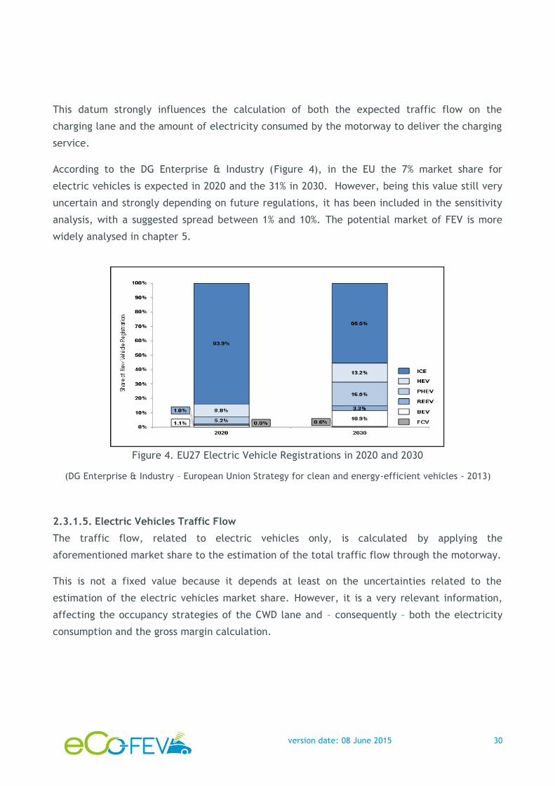
scenarios, by considering both the transport mode share and the market penetration.


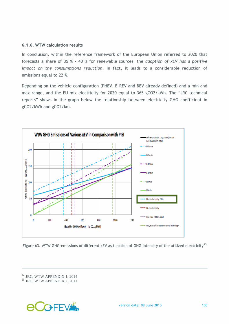
2. Impact assessment of charging technologies

Besides the evaluation of the eCo-FEV system based on experimental deployment and actual

testing, some components of the system are to be evaluated through simulations, as reported

in D400.1. Those simulation studies are focused mainly on the charging, energy consumption

and range aspects in electro-mobility, especially – yet not only - related to the use of charge

while drive concepts. A more specific analysis on the wired static charging, with related effect

on energy use, recharging time and generated queues in different conditions has been

reported in a specific report a part, for publication.

The input parameters for the simulation, characterising different configurations or test

scenarios, need to be well recorded together with simulation outputs for further analyses and

evaluation. It is also important to have synergies between the simulation study and actual

experimentation, so that:

the simulation parameters can be realistically set based on experiments and the actual

development;

the deployment can benefit from the simulation outputs and experiences.

The data recorded during the simulation studies are related to:

1. Analysis of electric vehicle usability. These data are related to the energy consumption of

different kinds of vehicles - private cars, light duty and heavy-duty ones - depending on the

mass and the type of vehicle. Together with that, the estimation of the range of energy

consumption and driving range are useful data. Here, we refer to typical distributions of

travels as those collected in literature in terms of frequency and distances run with private

cars; these data can be merged with analyses conducted by Politecnico di Torino,

concerning the use and distances daily covered by drivers. Given the estimated energy

consumption range, different aspects of the vehicle performances can be analysed.

2. Impact assessment of CWD performance in traffic flow scenarios concerning motorways

and urban applications.

3. Impact assessment of static electric charging on quality service in queues and energy

management. The main aim here is to assess the effect and sustainability of the static

charging as well as of the CWD.


The first point has been all explicated in one scientific paper1; the second and third points are

explained hereafter.

2.1. Impact assessment in parking areas for wired charging

2.1.1. Transport and traffic issues

This analysis has been faced in a deeper context with a specific report, which is not a

deliverable document, based on the impact assessment of static electric charging; this has

been analysed both on the quality service when queues are formed, and on the energy

management viewpoint.

The main aim here is to assess the effect and sustainability of the static electric charging on

traffic and queuing phenomena.

The model has been developed with the Matlab toolbox SimEvents, which provides blocks to

simulate discrete events, queues and servers. The model simulates a charging station with n

charging sockets during a complete day.

The first step has been to try to model the arrival of rechargeable vehicles - electric and plug

in hybrid ones - according to real patterns. The Matlab blocks generate entities following

common distribution functions, and with different characteristics, in terms of SoC, priority,

and the arrival hour. Depending on the arrival time a charging mode can be chosen. Then a

Matlab function takes over to calculate the necessary charging time based on the battery

capacity of the EV, besides the charging power and current, both direct or alternate, which

implies both solutions on board and with external charger.

This analysis has been focused on studying the possibility of using the hybrid or electric

vehicles in freight transport sector and concretely in urban distribution goods. The use of zero

emissions vehicles in urban freight distribution will suppose a considerable reduction in total

city emissions and therefore and improvement of air quality and a step to pursue with the

targets agreed in Europa 2020 strategy and other European directives. The first two chapters

are a review of the current state of electric vehicle technologies and the state of transport

sector in Italy, concretely the urban freight distribution. The following two are theoretical

1 See: Dalla Chiara B., Bottero M., Deflorio F.P., Filidoro I., “Competence Area of Electric Vehicles and Relevance of an ITS Support for Transport and Parking Issues”, in proceedings of the 21st ITS World Congress, Detroit, Michigan – USA, 7-11 September 2014.


researches, the first about the current competitiveness of electric vehicles for their use as

distribution vehicles, analysing different matters as current economic aspects and technical

characteristics, as well as future prospects. The second one about the potential impact of a

possible integration of electric vehicles into the grid.

Finally, a possible charging station model is simulated using MATLAB. In this model, behaviour

and schedules of different freight distribution vehicles is simulated in order to study the

potential and sustainability of a given charging station to supply an electric fleet. Times

needed to charging batteries and queuing phenomena are analysed with the purpose of

studying the competitiveness of these types of vehicles to perform goods distribution task

within time limits of the sector.

2.1.2. Forecasts and energy issues relate to marker forecasts

In order to provide a base for a forecast on future public charging stations, which will have to

be installed in the European Union by 20202, several studies have been examined, which offer

a wide range of forecasts.

Of course, areas where public charging stations have been installed will encourage possible

customers to purchase electric or a plug-in hybrid vehicle.

Some case studies have been analysed in order to identify the number of charging station

required: in particular a study of the consulting company Frost & Sullivan, one of the

University of Duisburg-Essen in 2012 for the city of Koln and surroundings.

2 Source: EC, COM(2010)186 final, A European strategy on clean and energy efficient vehicles; then o the 29th of September 2014, a new directive set a regulatory framework for the following fuels […]: “Electricity: The directive requires Member States to set targets for recharging points accessible to the public, to be built by 2020, to ensure that electric vehicles can circulate at least in urban and suburban agglomerations. Targets should ideally foresee a minimum of one recharging point per ten electric vehicles. Moreover, the directive makes it mandatory to use a common plug all across the EU, which will allow EU-wide mobility.” [http://ec.europa.eu/transport/newsletters/2014/10-03/articles/clean_fuels_en.htm]

http://ec.europa.eu/transport/newsletters/2014/10-03/articles/clean_fuels_en.htm

http://ec.europa.eu/transport/newsletters/2014/10-03/articles/clean_fuels_en.htm


1. A rather optimistic forecast has been performed by the consulting company Frost &

Sullivan.

It predicts the number of public charging points in Europe to reach 2 million by 2017. Frost &

Sullivan do not distinguish between the European Union and other European countries. It

therefore includes also European countries which are not part of the European Union.

Currently about 740 million people live in Europe, out of which 505.5 million live in the

European Union. According to the mentioned study, approximately 1.3664 million public

charging stations would be installed in the European Union by 20173. As the countries of the

European Union have a significantly larger average GDP per citizen than the European

countries which are not part of the Union, this number might be expected to be significantly

higher; as by 2017 electric vehicles will still be more expensive than vehicles with a

conventional engine and governments with high revenues from taxes (due to a higher GDP) are

more likely to subsidise the transition to electro-mobility. Therefore the number of public

charging stations in the European Union is (based on the findings of Frost & Sullivan) expected

to be about 1.7 million by 2017. As this forecast was performed in the year 2011 when less

than 10,000 public charging points were installed (using data from the year 2010), this would

mean that each year an average of about 282,000 new public charging stations would have to

be installed. Assuming that this trend continues until 2020 this would lead to approximately

2.5 million public charging points in the European Union.

2. A more conservative approach has been performed by the Berenberg Bank in co-

operation with the German “Hamburgisches Welt WirtschaftsInstitut”.

This study extrapolates the possible number of public charging stations in Germany to 10,000

by 2023, by adopting the same ratio ‘number of Charging station per citizen’ to the other EU

countries, the consequent total number of charging stations in the European Union can be

extrapolated to 53,350 or 0.053 million4.

3. The following scenario is similar to the results of a survey performed in Koln and

3 Deutsche Stiftung Weltbevolkerung 4 Nationale Plattform Elektromobilitat


surrounding cities in 2011 by the Chair of General Business Administration &

International Automotive Management by Professor Dr. Heike Proff of the University of

Duisburg-Essen.

About 2,600 citizens in six cities or rural districts in and around Koln have been questioned

(900 of those in the city of Koln) about their preferences concerning several issues, which are

of high importance for the transition to electro-mobility. One of these important issues is the

preference concerning the location to recharge an electric vehicle.

A study made on a questionnaire to Koln citizens found out that:

- 56.3 % of the questioned would charge their vehicle at home

- 67 % would recharge their vehicle at their working-place

- 49.1 % consider a public charging station as attractive

- 21.3 % would use a service comparable to today’s petrol stations.

The same trend has been detected for the other cities in which the survey has been

performed:

- The willingness to use public charging stations differs within the range of 39.2 % in

Bochum and 56.2 % in Duisburg;

- only 46.05 % of the questioned citizens in cities close to Koln consider the occasional

use of public charging stations as attractive;

- 54.2 % would prefer to charge their vehicle at home

- 62.65 % reported they would use charging stations at their workplace.

In rural areas this trend is even clearer:

- 26.3 % of the questioned citizens' found public charging stations attractive;

- 87.2 % would utilise the possibility to charge their vehicle at their workplace;

- 88.5 % would charge their vehicle at home.

This deviance can be explained by the higher percentage of citizens who own their own house

in rural areas.


For the providers of public charging stations the number of users who are likely to use their

offers on a regular basis is of high importance, as only such users make the installation of

charging stations – especially in residential areas – an economical attractive business.

To perform an approximation about the necessary number of public charging stations in the

analysed areas, the percentage values are therefore divided by two, as each user has on

average given two answers. However it is not likely to recharge an electric vehicle more than

once a day, given the average driving distance of about 43 km per day.

Therefore about 25 % of the questioned citizens are likely to use a public charging station on a

regular basis (assuming that within 2030 most EV will be sold and used in urban areas).

As it is likely that some users who would not use public charging stations on a regular basis

would still use public charging stations on the weekend or on a non-regular basis (e.g. when

visiting friends in other cities) it is assumed that on average 30 % of all electric vehicles would

be recharged at public charging stations on a normal day. It is there assumed that this number

might be representative for the whole European Union.

While users can charge their cars at home without facing major problems or costs and may also

be able to charge their car at their company’s or at semi-public charging stations (e.g.

supermarkets) in the near future, users who live in cities and therefore do not possess their

own parking place are dependent on the availability of public charging stations.

Economic impact assessment

According to the National Plattform Elektromobilitat, a 2011 study shows that the costs for

the installation of a public charging station are estimated from 4.700 to 9.000 Euro.

Another report made by AVERE - European Association for Battery, Hybrid and Fuel Cell

Electric Vehicles - shows the following data:

1) The current average price for a 2-plug (2 x (IEC 61851-1) Mode 3 plugs) charging station can

vary from 4.000€ to €5.000 depending on where in Europe and how smart the station is. A fast

charging station costs around €25.000.

2) The installation costs of a charging station will vary depending on:

- “building” costs (for example if digging is necessary)


- costs of the parking space, road signs, marking, communication, etc.

The costs of public charging infrastructure should be split into two elements: the actual costs

of the charging stations and the costs of installation of the charging stations that are variable

depending on location, availability of power, conduit size and labour.

Regarding the cost related to the parking space in city centres, this could be quite relevant,

for example in Slovenia it can be up to €15.000. The connection fees to the grid will also have

to be paid to the DSO (Distribution System Operator) and again this can be up to €1.000 per

plug.

Therefore the cost of the charging station itself is very often 1/2 or 1/3 or even 1/4 of the

overall costs. After installation, maintenance costs should also be taken into account and

these could be up to €2.000 per charging station per year.

While the costs for Domestic charging infrastructure should be as follows.

To estimate those costs, the number of predicted EVs should be multiplied by at least 2 to get

the number of plugs needed (at home, at work...). There are currently two possible solutions.

1) CEE16A-plug: The estimated total cost for a simple installation with a CEE16A- plug

including a protection device and a simple electronic device for communication lasting for 10

years is € 100.

2) Home Charge Device (Wall box solution): The estimated cost for a Home Charge Device /

Wall Box solution is a bit more expensive: around €400.

This installation would probably have to be replaced after 5 years following the technological

appliance obsolescence.

Another study has been performed by EURELECTRIC - Union of the Electricity Industry - where:

2 Plug Station (2x max. 22kW AC, Smart Charging compatible) ~ 5.300 €

2 Plug Station (2x max. 11kW AC) ~ 2.500 €

1 Plug Box (1x max. 22kW AC, Smart Charging compatible) ~ 1.900 €

1 Plug Box (1x max. 11kW AC) ~ 500 €


DC Fast Charging Station ~ 40.000 €

Connection Costs:

- AC Range: 1.850 € - 5.200 € (Depending on max. capacity and cable length up to 10m)

- DC Range: 4.000 € - 13.300 €

Recharging an electric vehicle means charging the battery. Hence the “fuelling” of an electric

vehicle will depend on the combination of:

• charging power (i.e. the voltage/amperage and the number of phases of the plug)

• battery characteristics

By considering the Frost and Sullivan study mentioned before that lead to approximately 2.5

million public charging points in the European Union by 2020 and multiplying it by the average

cost, then the investment needed follows here.

Considering that a Mode 3 charging station with two plug-ins cost from 4.000 to 5.000 € in

2011, thanks to economies of scales, it can be approximated to 3.000 €. Also the installation

and connection costs can decrease due to economies of scales up to 3.000 €.

Average cost for a 2 plug-in station = 3.000 € + 3.000 € = 6.000 €

2.5 million are public charging points: 2.5 / 2 = 1.25 million 2-plug charging stations.

The cost of the 2-plugs stations themselves is:

1.25 million * (6.000 €) = 7,5 Billion €

This is the investment required according to the basic calculus made on rough approximation,

but a quite good tool to work with.


2.2. Impact assessment of CWD on selected traffic flow scenarios

As mentioned, results for the impact assessment of a CWD service on traffic are based on

simulation. Two different scenarios have been simulated: the first (a) is related to a motorway

with a dedicated charging lane, whereas the other (b) explores the possibility to equip with a

CWD an urban arterial. A degraded solution, much easier to apply, is the charging in parking

areas similar to a “pit stop”, yet not analysed hereafter being a simpler case than the more

complex reported hereafter.

a. The Electric Vehicle Supply Equipment (EVSE) of the CWD technology is

macroscopically designed on the basis of a simplified model. The analysis could be applied to a

roadway scenario with three lanes, where the right-hand lane is reserved for the wireless

charging activities. Data are related to the CWD lane, a balance between the energy

consumed for vehicle motion and the energy provided by the charging zones in order to

evaluate the SOC of the vehicles batteries. The model used for estimating the vehicles

consumptions is based on the resistances to motion. The energy received from the vehicle by

a coil is strictly related to the dimension of the elements of the system (coil and on-board

device), to the power provided and to the occupancy time. During the simulation experiments,

a reference scenario is set according to the preliminary analysis reported in the section 2.3.2.2,

by individuating the most adequate layout for charging zones length, their inter-distance and

the power provided for the selected vehicle. Furthermore, a second scenario is explored in

order to analyse how the system performances could be affected by the increase of both the

FEV traffic and the minimum allowed technical headway on the CWD lane. After defining the

CWD layout, it is useful to estimate the quality level for the charging service and the type of

distribution of the electrical power, which should be supplied at each node. This implies an

implementation of the model for the simulation of the traffic flow along the road as defined

previously.

In the WP440 activities, traffic and energy results have been analysed in two different

operational scenarios.


The CWD system is also applied to a multilane ring road with several intermediate on-ramp

entrances, where the slowest lane is reserved for the charging activities, when authorised

vehicles are present; a similar case would be the use of the segregated lane for public

transport in a urban context, where electric public transport absorbs electric while operating

or during stops, at the bus stops or at the traffic lights, but even taxi-cabs or few other

electric vehicles might make use of this recharging opportunity.

A specific traffic model has been developed and implemented adopting a mesoscopic traffic

modelling approach (described in the section 2.3.2.5), where vehicle energy needs and

charging opportunities affect drivers’ behaviour. Overtaking manoeuvres, as well as new

entries in the CWD lane of vehicles that need to be charged, have been modelled by taking

into account a fully cooperative driving system among vehicles which manages an adequate

gap between consecutive vehicles. Finally, a speed control strategy in which vehicles can be

delayed to create an empty time-space slot in the CWD lane, is simulated at a defined node.

b. A method based on traffic micro-simulation on Charge-While-Driving systems for fully

electric vehicles in urban environments is applied for the impact assessment in this scenario.

The examined CWD solution is deployed by charging zones, which are installed before the

stopping lines at signalised intersections. The opportunity to charge an electric vehicle en

route is provided for almost stationary vehicle conditions, when it may be in queue for

junction control requirements. The analysed scenario refers to a 2-km urban arterial with

eight signalised intersections, where 10% of the traffic is assumed being electric vehicles. CWD

performance results are reported from the viewpoints of both driver and energy provider.

2.3. Impact assessment of CWD on motorways

To assess the CWD impact, a simulation scenario is performed to show its potential to enable

full electric mobility. From the motorway operator’s perspective, CWD might be an interesting

added service to be provided to customers, enabling them to use the motorway infrastructure

without worrying about charging issues. The implementation of the dynamic recharging

requires to identify and to develop an integrative operator platform able to connect and

exchange information with road IT infrastructure, road side infrastructure, On Board Units

(OBUs) integrated in the electric vehicles, and charging network operators. According to this


point of view, the motorway concessionaire could be the candidate both to manage the eCo-

FEV “operator platform” and to invest in the construction of the charging infrastructure.

The simulation tool, developed by POLITO, has been adapted to a possible future business

scenario and can receive input data as close as possible to real operating conditions (i.e. daily

distribution of traffic, number of FEVs circulating on the motorway, vehicle SOC levels,

charging strategies…).

Its main output can be, as well as traffic performance on the CWD lane, also the total energy

consumption required by the motorway to deliver the charging service on a certain time period.

The simulation covers one day and the extension for wider periods can be done using the

output results and extended traffic data. Starting from this datum, a preliminary analysis of

the gross margin - generated by the charging service – can be delivered. The aim of this study

is to assess the target of the maximum level of investment cost, allowing the adoption of the

CWD technology in the market, without either incentive policies or financial aids. It must be

noticed that, in a real business scenario, CWD might be enhanced through specific policies.

However this evaluation goes far beyond the scope of the present study and might be even

premature, because of the many uncertainties related to a non-market technology.

2.3.1. CWD Business Model for Motorway Concessionaires

A possible business model, enhancing the adoption of CWD technology by motorway

concessionaires, might be described as follows.

The CWD service is:

a. Provided by the motorway operator;

b. Managed through the eCo-FEV platform;

c. Delivered to each electric vehicle driver.

The motorway operator:

− owns and manages the CWD charging infrastructure integrated in the lane;

− owns and manages the eCo-FEV platform as a component of its own ITS system;

− manages the charging service (i.e. facility booking, electricity delivery, billing through

the toll payment);


− supplies electricity from the energy provider, acting at the aggregated level of the

motorway power grid.

On the perspective of the motorway concessionaire, it would be certainly useful to support

future investment decisions about CWD solution through the development a specific business

plan. However, at this step of the research, the CWD technology is still very far from a market

application and too many uncertainties are likely to deeply affect a precise economic

evaluation. A good business plan requires at least a certain knowledge about several input

data: investment costs, depreciation rates, ordinary and extraordinary maintenance plans,

revenues model, revenues cash flow, management and operational costs. Despite of these

limits, a first estimation of the CWD economic impact may still be useful, at least to provide

to motorway concessionaires a general picture about the future scenario. To this purpose, a

sensitivity analysis has been developed, with the aim to enlighten the most relevant

parameters affecting the CWD market development, as far as motorways are concerned. As

detailed in the following sections, the analysis will be based on the estimation of the gross

margin generated by the charging service and the evaluation of a possible upper limit in

investment costs.

2.3.1.1. Reference Period

The first issue to be addressed is the choice of the reference period, because - as explained in

the following sections – this information affects many other parameters (i.e. number of

electric vehicles driving through the motorway). Considering that the CWD technology is still a

non-market solution and its adoption in the motorways sector will easily require a wider

diffusion of electric vehicles, a 2020 - 2030 scenario should provide a proper business

landscape for developing the aforementioned sensitivity analysis.

2.3.1.2. Time Period

To properly assess the CWD economic feasibility, the reference time period is assumed to be

one year, based on a detailed representation of a typical daily traffic data. The level of time

resolution for traffic data profile can be assumed equal to 1 hour, as the availability of this

type of data is more frequent. An example of this traffic distribution can be found for the UK

roads and reported in Figure 3 where the average traffic index is depicted for various days.


Figure 3. Distribution of traffic flows by time of the day and days of the week. UK, 2013

2.3.1.3. Motorway typical scenario

A general road section of about 20 km of motorway has been considered, being this the

average distance between two motorway exits. The motorway section is assumed to have

three lanes, as mentioned: charging vehicles have to move to the farthest right lane, hosting

the CWD solution. The power transfer efficiency is assumed equal to 85%.

More detailed data on this scenario can be found in the section 2.3.2.1.

2.3.1.4. Electric Vehicles Market Share

In a 2020 scenario, where CWD technology is expected to enhance full electric mobility, the

percentage of electric vehicles driving through a motorway might be assumed equal to their

market share.

0

50

100

150

200

250

00:00 03:00 06:00 09:00 12:00 15:00 18:00 21:00

Ind

ex

: A

ve

rag

e h

ou

r o

f th

e d

ay

= 1

00

Time (hour beginning)

Monday

Midweek

Friday

Saturday

Sunday


This datum strongly influences the calculation of both the expected traffic flow on the

charging lane and the amount of electricity consumed by the motorway to deliver the charging

service.

According to the DG Enterprise & Industry (Figure 4), in the EU the 7% market share for

electric vehicles is expected in 2020 and the 31% in 2030. However, being this value still very

uncertain and strongly depending on future regulations, it has been included in the sensitivity

analysis, with a suggested spread between 1% and 10%. The potential market of FEV is more

widely analysed in chapter 5.

Figure 4. EU27 Electric Vehicle Registrations in 2020 and 2030

(DG Enterprise & Industry – European Union Strategy for clean and energy-efficient vehicles - 2013)

2.3.1.5. Electric Vehicles Traffic Flow

The traffic flow, related to electric vehicles only, is calculated by applying the

aforementioned market share to the estimation of the total traffic flow through the motorway.

This is not a fixed value because it depends at least on the uncertainties related to the

estimation of the electric vehicles market share. However, it is a very relevant information,

affecting the occupancy strategies of the CWD lane and – consequently – both the electricity

consumption and the gross margin calculation.


2.3.1.6. Electricity Consumed by the Motorway

The electricity consumed by the motorway is calculated by increasing the electricity

transferred to the electric vehicles (EV) of the average loss percentage assumed for the CWD

solution.

Having assumed – before having the results of tests in the laboratory of POLITO (§ 3.4.3) - the

CWD power transfer efficiency about 85%, the electricity consumed by the motorway (EM) is

assumed as follows:

EM = EV / 0,85

2.3.1.7. Electricity price (motorway concessionaire vs energy provider)

The average electricity price, applied by the energy trader to the motorway concessionaire

(PM), is calculated starting from the key findings of the study “EU Energy, Transport and GHG

Emissions – Trends to 2050” (European Union - 2014) (Figure 5).

As regards electricity pricing, this report provides relevant information, such as:

− the projection of the electricity bill, by sector and before taxes

− the projected breakdown of the average electricity cost.

The motorway concessionaire is likely to be included in the “Industry” sector with an expected

2020 pre-tax cost about 115 Euro/MWh.

According to the study, operational tax and VAT on electricity can be calculated as 13% of the

pre-tax price. Therefore, the average cost of electricity (after tax) can be about 130

Euro/MWh (Figure 5, Figure 6).

Figure 5. Price of Electricity (pre-tax) by sector

(European Union – EU Energy, Transport and GHG Emissions – Trends to 2050 - 2014)


Figure 6. Cost Components of Average Electricity Price (European Union – EU Energy, Transport and GHG Emissions – Trends to 2050 - 2014)

2.3.1.8. Electricity Cost

The total annual cost (C) paid by the motorway concessionaire to the energy provider is

calculated by applying the aforementioned electricity price (motorway concessionaire vs

energy provider) to the electricity annually consumed by the motorway.

C = PM * EM

2.3.1.9. Electricity Delivered through the CWD Service

The electricity delivered to the electric vehicles (EV) driving along the CWD lane is calculated

by the simulation tool. This result depends on several input data (traffic flows, the charging

strategies, power transfer efficiency…) and – together with the electricity consumed by the

motorway (EM) – it is one of the main points of the sensitivity analysis.


The result of the simulation tool is the amount of energy consumed during the average day (EV

Day). The total yearly amount is calculated applying this value to each day of the year, without

considering the effect of possible weekly / seasonal fluctuations.

EV = EV Day * 365

2.3.1.10. Electricity price (electric vehicles vs motorway concessionaire)

The average electricity price, applied by the motorway concessionaire to the CWD customers

(PV), is calculated starting from the key findings of the study “EU Energy, Transport and GHG

Emissions – Trends to 2050” (European Union - 2014).

The CWD customer might be represented either by “households”, i.e. passenger vehicles, or by

“services”, i.e. freight distribution services, or even by “industries”, i.e. corporate fleets.

Therefore, it is likely that the charging service will be offered according to different revenues

schemes and pricing levels, depending on the final customer. At the moment it is difficult to

foresee which criteria will be chosen by motorway concessionaires. A cautionary assumption

might be based on the estimation of the average price of electricity in 2020. According to the

study “EU Energy, Transport and GHG Emissions – Trends to 2050” (European Union - 2014)

(Figure 5), this pre-tax value might be expected at about 150 Euro/MWh.

As already mentioned, exercise tax and VAT on electricity can be calculated as 13% of the pre-

tax price. Therefore the average price of electricity (after tax) can be about 170 Euro/MWh

(Figure 6).

2.3.1.11. CWD Revenues

The annual revenues (R) generated by the CWD service are calculated applying the

aforementioned electricity price (PV) to the amount of electricity annually consumed by the

electric vehicles (EV).

R = PV * EV

2.3.1.12. CWD Gross Margin

The gross margin (G), generated by the CWD service, is calculated as the difference between

CWD Revenues and CWD Costs. Because of the many uncertainties on the investment side, it is

not possible to estimate the impact of ordinary maintenance costs, directly or indirectly

related to the CWD solution (i.e. maintenance of the coils, additional maintenance costs of the


motorway infrastructure…). Therefore, the following calculation might overestimate the gross

margin value:

G = R - C

2.3.1.13. CWD Depreciation Rate

To properly evaluate the investment cost according to the gross margin, the CWD depreciation

rate (DR) should be known or at least estimated. At the moment, it might be difficult to know

the technical duration of a CWD apparel. However, being this latter composed at least by two

different elements – the electric plant and the ICT system - a cautionary estimation might be

based on the depreciation rate usually applied to software solutions, equal to 20%.

2.3.1.14. CWD Investment Costs

At the moment, investment costs (I) are poorly documented because CWD technology is still a

non-market solution. According to recent studies, the investment can vary in the range

between few hundred thousand euros per kilometre and a few million euros per kilometre

(Elektroborse Smarthouse - Wirelessly Charge Electric Vehicles by Induction While Driving -

2014).

Because of the many uncertainties, the CWD investment cost is not an input datum but it is

calculated as a break-even value based on the gross margin generated by the CWD service in

the depreciation period:

I = G/ DR

It must be underlined that the real investment target might be lower than this value, because

an Internal Rate of Return higher than zero should be considered. On the contrary, yearly

fluctuations on commodity prices may have either positive or negative effects on the gross

margin.

The previous considerations have not been included in the study because, due to the many

uncertainties, the most significant output should only be the investment size and not its

precise value.

2.3.2. Simulation model for the EVSE management and scenario description

To provide a clear framework for possible applications of the presented analysis, the model

developed could be applied also to a freight distribution service, for example. The FEV traffic

http://www.elektroboerse-smarthouse.de/elektroinstallation/elektromobilitaet/artikel/104848/


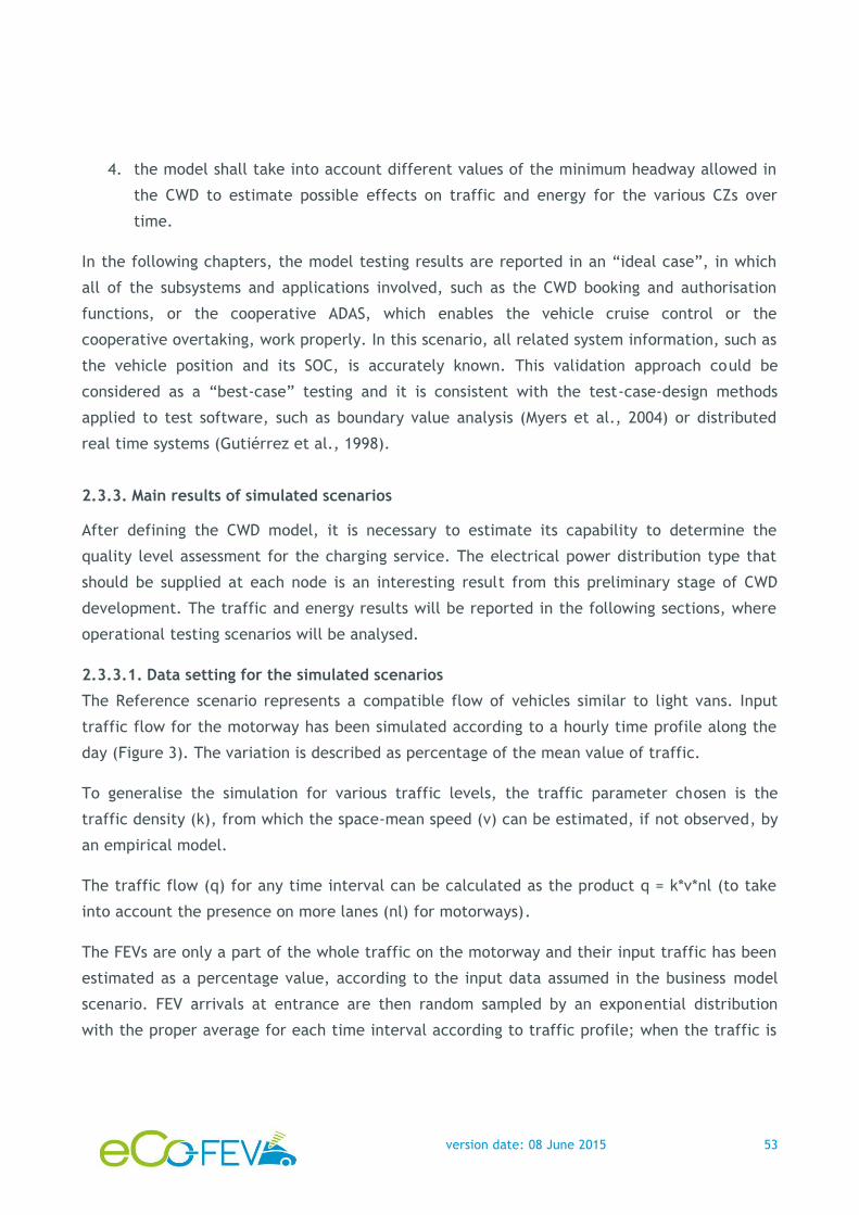
flow simulated here represents a fleet of light vans that could be generated by, or directed to,

a logistics centre for a distribution service. In the analysed case, the service can be planned

and vehicles can have a common route segment, although they can perform multiple

deliveries. The fleet management in this case could include the CWD usage in the common

route segment to allow vehicles to cover greater distances, avoiding slack time for a stationary

recharge .

2.3.2.1. Models for energy estimation

In the CWD lane, a balance between the energy consumed for vehicle motion and the energy

provided by the charging zones (CZs) should be established to monitor the SOC of the vehicle

batteries during the observation period. The vehicle types included in the traffic flow is

relevant because their mass and their aerodynamic parameters affect the energy consumption.

The analysis is applied to a 20 km roadway with multiple lanes scenario. The right-hand lane is

reserved for the charging activities. In an actual road infrastructure example, this solution

could be applied by allocating the slowest lane to CWD operations or by using the emergency

lane with dynamic lane management. Figure 7 shows a CWD lane scheme, with two CZs

represented. The EVSE includes inductive coils placed under the pavement surface, at a

relative distance, which generate a high frequency alternating magnetic field to which the coil

on the car couples and power is transferred to charge the battery.

Figure 7 .Scenario layout for CWD in a road with three lanes

The model used for estimating the vehicle energy consumption is based on the resistance to

motion. The total resistance (Rtot) is given by the following relationship:

Rtot = Rdrag + Rrolling + Racceleration + Rslope

LCZ I

Charging Lane


Where:

𝑅𝑑𝑟𝑎𝑔 =1

2∙ 𝜌 ∙ 𝑐𝑥 ∙ 𝐴 ∙ 𝑆2

ρ: air density [kg

m3]

cx: drag coefficient

A: cross sectional area [m2]

S: vehicle speed relative to the air [m

s]

𝑅𝑟𝑜𝑙𝑙𝑖𝑛𝑔 = 𝑚 ∙ (𝑓0 + 𝑓2 ∙ 𝑠2)

m: vehicle mass [kg]

f0: coefficient [m

s2] that considers the characteristics of the road surface

f2: coefficient [1

m]

s: vehicle speed [m

s]

𝑅𝑎𝑐𝑐𝑒𝑙𝑒𝑟𝑎𝑡𝑖𝑜𝑛 = 𝑚 ∙ 𝑎

a: vehicle acceleration [m

s2]

Rslope = m ∙ g ∙ p

g: gravity acceleration [m

s2]

p: average slope of the road

After calculating the resistance to motion, the power consumed is calculated as follows:

𝑃𝑒𝑙𝑒𝑐𝑡𝑟𝑖𝑐 =𝑅𝑡𝑜𝑡 ∙ 𝑠

η𝑑+ 𝑃𝑎𝑢𝑥

Where ηd is the driveline efficiency. Paux is the auxiliary power that includes all consumption

not related to the vehicle motion, such as the on-board electrical devices (e.g., lights and air

conditioning). The parameter values used in these scenarios are reported in next sections.

Finally, the energy consumed by the vehicle over time is obtained by multiplying the power

consumed by the duration. In our scenarios, for sake of simplicity, the average slope will be

assumed to equal zero.


The energy that the vehicle receives from a coil is strictly related to the system element

dimensions (CZs and on-board devices), the power provided per unit of length (Pcz) and the

occupancy time.

When the vehicle crosses a transmitting coil, it receives the energy according to a system

efficiency (ηs) that depends on the distance between the coil(s) of the on-board device and

the coil(s) of the CZ installed in the road pavement. A transition coefficient (Trk) is introduced

to account for the initial and final partial overlaps by decreasing the actual CZ charging length

(LCZ) as follows:

LCZeff = LCZ − Trk ∙ LCD

Trk accounts for the reduction in the actual energy received from each CZ. This energy

depends on the occupancy time (t) and is related to the vehicle speed on the CZ as follows:

En = t ∙ Pcz =LCZeff

s∙ Pcz ∙ LCD ∙ ηs

Each CZ is subdivided into coils that are excited only if a receiving - and authorised- vehicle is

above them. In this way, only the coils that are under the vehicle work, thus maintaining the

emitted power inside a shielded zone, corresponding to the vehicle occupancy.

2.3.2.2. Setting of CWD design parameters

The indicator used to design the layout of the charging infrastructure is the difference

between the final and the starting EV battery SOC5 (∆SOC) after 1 km in the CWD lane. Figure

8 and Figure 9 respectively show, for the considered light-van (vehicle parameters are

reported in Table 1), empty and full loaded conditions and how the energy variations (∆SOC)

are related with the changing of three main parameters: LCZ (from 10 to 50 m); I (from 20 to

100 m); and the EV speed (from 20 to 80 km/h). A CWD system efficiency ηs of 85% is here

assumed for any power level to simplify the analysis.

5 In literature, the term SOC is generally used to define the battery state of charge as percentage unit being a state or a ratio of charge. As a matter of fact, our analyses needed to deal with energy variations by monitoring the Level of Charging (LOC) or even a SOC, yet related to accumulated energy in a battery. This last corresponds to the energy stored expressed in kWh and not in %, a value that can be obtained by multiplying the SOC [%] by the battery Capacity [kWh], which is approximately a constant given a certain vehicle. This means that hereafter the SOC is actually a LOC or a kSOC or even an absolute SOC of a specific battery. We excuse ourselves for the confusion that this might arise to the Reader.


Table 1. Electric light van data

Variable Value Unit

Mass 2500 kg

Frontal area 4.9 m2

Cx 0.38

f0 0.12 m/s2

f2 0.000005 1/m

Driveline efficiency (η𝑑) 0.75

Auxiliary power (Paux) 0.8 kW

Figure 8 Scenarios explored for the electrical light-van in EMPTY CONDITIONS (2500 kg)

Taking into account the results obtained by the developed analysis, a correct design procedure

should consider, on the one hand, the service provider’s need to minimise the installation and

maintenance costs and, on the other hand, users’ acceptance of the travel time required for a

proper recharge in the CWD lane.


The speed has a relevant influence on the results. Considering the test vehicle in empty

conditions, the design hypothesis on the speed in the CWD lane assumes two different allowed

speeds in the CWD lane: the highest one allows the vehicle to maintain its entering SOC, while

the second one is a compromise between the recharge need of vehicles with a low SOC and a

minimum speed that can be accepted by the users. Assuming the highest speed is equal to 60

km/h, the equilibrium between the energy consumed and the energy provided by the coils is

obtained with a percentage of the equipped lane of 40% (LCZ = 20 m, I = 30m, ∆SOC = 11 Wh).

In this layout, assuming the lowest speed is equal to 30 km/h, after 1 km, the user obtains an

increase of the battery energy stored of 367 Wh, which means that to obtain an energy

increase of 1 kWh, the vehicle needs to cover approximately 2.7 km in the CWD lane.

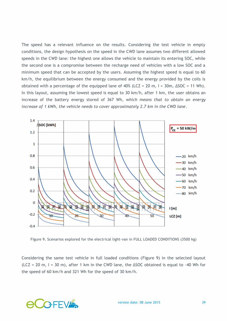
Figure 9. Scenarios explored for the electrical light-van in FULL LOADED CONDITIONS (3500 kg)

Considering the same test vehicle in full loaded conditions (Figure 9) in the selected layout

(LCZ = 20 m, I = 30 m), after 1 km in the CWD lane, the ∆SOC obtained is equal to -40 Wh for

the speed of 60 km/h and 321 Wh for the speed of 30 km/h.


2.3.2.3. Verification of the CWD system for an electrical city car

The setting of the CWD system parameters previously described has been defined according to

the characteristics of a light-van, as the charging system has been specifically designed for a

freight distribution service connecting the city and the logistic centre. However, the same

charging system may be used by different electric vehicles if they are equipped with a

compatible on-board device. For instance, city cars have lower masses, and the energy

balance between the consumption and the energy received from the road will consequently be

different. Therefore, an evaluation of the effects of the adopted CWD system on the ∆SOC of a

city car will be carried out, considering a vehicle whose characteristics are reported in Table

2.

Table 2. Electric city car data

Variable Value Unit

Mass 1600 kg

Frontal area 2.229 m2

Cx 0.336

f0 0.12 m/s2

f2 0.000005 1/m

Driveline efficiency (η𝑑) 0.75

Auxiliary power (Paux) 0.8 kW

Taking into account the smaller dimensions of the city car, perhaps an LCD of 1 m could not be

adopted, although this issue should be addressed in the future by car manufacturers. For this

reason, the analysis is developed by individuating the trend of the ∆SOC with various options

of LCD and different speeds (Figure 10), according to the EVSE settings previously defined (LCZ

= 20 m, I = 30 m, Pcz = 50 kW/m).


Figure 10. Influence of speed and LCD on the ∆SOC for an electrical city car for the adopted EVSE settings, after 1 km

Considering the higher design charging speed, which guarantees to the vehicle the maintaining

of its SOC, as previously defined, Figure 10 shows that almost the same energy variation

(∆SOC) results of the light-van can also be obtained for the city car, albeit driving at a higher

speed.

In detail, adopting the same value of the LCD (1 m) as the light-van, a ∆SOC of 18 Wh is

obtained for a speed of 80 km/h, while for the light-van, a ∆SOC of 11 Wh was obtained for 60

km/h.

However, considering the lower charging speed introduced for low SOC vehicles, a result for

the ∆SOC comparable with that of the light-van is obtained with a smaller increase in the

vehicle speed (a ∆SOC of 287 Wh for a speed of 40 km/h and a ∆SOC of 426 Wh for a speed of

30 km/h, while for the light-van, a ∆SOC of 367 Wh was obtained for a speed of 30 km/h). In

fact, as previously described, the relationship between the energy received by the vehicle and

its speed is linear because it depends on the CZ occupancy time, while the energy consumed

by the vehicle along the travel is proportional to the third power of its speed. In the case of


this new test vehicle, a reduction of the mass and an improvement of the aerodynamic

parameters (Cx and frontal surface) are introduced. Therefore, because of the non-linear

relationship between the vehicle consumption and its speed, these three parameters influence

sensibly the vehicle consumption for high speeds.

The non-linear relationship also affects the choice of different LCDs. If the same charging

speeds defined for the light-van would be adopted for the city car, the LCD could be reduced

to 0.5 m to maintain the SOC in the CWD lane driving at 60 km/h (∆SOC = -4 Wh after 1 km).

With this LCD value, however, after 1 km driving at 30 km/h, the ∆SOC obtained (164 Wh) is

about half that obtained by the light-van equipped with an on-board device of 1 m (321 Wh).

Alternatively, assuming, for example, an LCD of 0.9 m, the speeds can be increased up to 80

km/h to preserve the SOC (∆SOC = -1 Wh) and 50 km/h (∆SOC = 165 Wh) to obtain a relevant

charge.

2.3.2.4. Preliminary test of energy benefits for CWD in the selected design scenario

A proper design procedure should consider both the service provider’s need to minimise the

installation and maintenance costs and the users’ acceptance of the time required for a proper

recharge in the CWD lane. Taking into account the results obtained in the previous section

(more details are reported in [10]) for an electric light van, with a Pcz of 50 kW/m in the CZs

and adopting a ηs of 85% (from energy grid distribution to EV battery), the identified CWD

system can be described by the following technical requirements:

− Length of the charging zones (LCZ) = 20 m;

− Inter-distance (I) = 30 m;

− Longitudinal dimension of the on-board charging device (LCD) = 1 m.

To verify the charging infrastructure performance, it is useful to analyse how the energy

balance of the vehicles changes with their speed (Figure 11). Figure 11 illustrates that the

energy equilibrium is possible at 60 km/h, whereas at lower speeds the SOC gain is positive. To

avoid frequent potential collisions between vehicles and consequent overtake manoeuvres, the

speed on the CWD lane cannot be unrestricted. The speed should be set according to charging

and travel time needs. The average speed should be constant along the CWD lane, except for

local interactions. For this reason, even the acceleration resistance can be neglected. The two

following operational speeds can be defined for CWD: the highest speed (60 km/h) should

allow the vehicle to maintain its entering SOC, whereas the other speed (30 km/h) should be a

compromise between the recharge needs of vehicles with a low SOC and a minimum speed that


can be accepted by the users. In this layout, by driving at the lowest speed, after 20 km in the

CWD lane the SOC increases by more than 7 kWh. This last case has been defined as “emer”

status because this refers to a strategy applicable to emergency situations. The other charging

vehicles have been labelled with the “charge” status.

Figure 11. Positive and negative energy for the empty electrical light-van (2500 kg) after 20 km in the charging lane, at different speeds for the selected CWD layout (LCZ= 20m, I=30m)

2.3.2.5. Traffic modelling

The choice of the traffic modelling is derived from the specific requirements of the CWD

system (eCo-FEV, 2013) as synthesised below:

1. it has been assumed as installed only along the right-hand lane of the motorway

because that lane is generally used by slower vehicles; consequently the model

considers the lane disaggregation of traffic data;

2. the charging lane can be used for two different charging needs (“emer” or “charge”)

corresponding to two different vehicle speeds; consequently, the model must consider

different classes of vehicles.

One possible approach to effectively model this type of problem (multilane and multiclass)

could be micro-simulation, in which single vehicle trajectories are modelled with a small time

step resolution and with their interaction on the road. An extensive review of traffic modelling


approaches can be found in Hoogendoorn and Bovy (2001)[13], whereas a micro-simulation

model application example is reported by Barceló et al. (2005)[15]. Although the micro-

simulation approach meets the principal requirements of the traffic model for CWD, it does

not model vehicle behaviour according to their energy needs. The current SOC level of the

vehicles and the fleet operators' eventual SOC target requirements influence drivers’ decisions

concerning lane changing behaviour, i.e., vehicles try to enter into the charging lane or to exit

according to their needs. Therefore, specific rules must be defined and implemented to obtain

realistic results from the traffic model. In addition, the detailed rules implemented in a micro-

simulation model usually require an accurate calibration process, aimed at replicating actual

driver behaviour in traffic. However, the calibration process can be compromised in a CWD

scenario whenever various ADAS are available on-board because they affect driving and traffic

behaviour.

Consequently, a mesoscopic approach would be more accurate than a microscopic one,

because the latter is too detailed for this preliminary stage of CWD technology. Further

comments on this issue will be reported in Section 2.3.2.7.

A framework of mesoscopic traffic models can be found in Cascetta (2001)[16], whereas a

recent application of this type of model was proposed by Ben-Akiva et al. (2012)[17].

The developed model represents single vehicle trajectories without introducing a detailed

time resolution of the driving behaviour. It assumes that the CWD lane conditions can be

described knowing only the data related to consecutive points. The point spacing, typically

hundreds of meters, can be set based on the analysis required. For this reason, detailed traffic

information has been updated only at these defined points, defined as “detection points” or

“nodes”, where it is interesting to know the time series of traffic parameters and the energy

provided for the entire vehicle set detected in the related time period. The road segment

between the consecutive nodes will be defined as “road section” or “section”. Aggregated

traffic information, such as average headways, delays and the number of overtake

manoeuvres, can be estimated along the CWD lane for any road section. The logic scheme

adopted for two consecutive nodes of the traffic model is depicted in Figure 12.


Figure 12. Several trajectories in the time-space diagram to trace the arrival times of different vehicle types at consecutive nodes.

In the traffic model, the arrival time of a vehicle at the node (i) is first estimated based on its

arrival time at the node (i-1) and its desired speed. It is then adjusted, in a second step,

according to the feasible headway for vehicles in the lane (headway min). Because of safety

and possible technical reasons, a headway less than a threshold value between two vehicles in

the charging lane may not be allowed. If two vehicles detected at a certain node are too

close, in terms of headway, the following one has to slow down until its headway is equal to

the threshold. The headway verification and correction is therefore performed only at discrete

space steps, according to the mesoscopic modelling of vehicle behaviour. In an actual

scenario, it can be managed by drivers or by the cooperative system adapting the vehicle

speed along the entire section before the node where the headway adjustment is performed.


The battery SOC, monitored along the road at each node, plays a crucial role because it

influences drivers’ decisions to use the CWD service or not. It is also the parameter used to

divide the vehicles into different speed classes. In the model, the CWD lane entries are

managed according to the following cooperative behaviour: each vehicle requiring recharge

moves into the CWD lane at the node, creating the necessary gap in the vehicle flow by

slowing down the following vehicles.

The proposed scenario refers to a freight distribution service; the decision to charge may be

simplified because it depends not only on drivers and their final destinations, but primarily on

the fleet operator. To restart the delivery operations in the second part of the day, all of the

vehicles in the fleet may require an energy level adequate for their operation.

The analysis considers even the overtaking cases: a cooperative overtaking model at constant

speed is implemented and the vehicle does not recharge while it is outside the charging lane.

An example of a highway automation system cooperative scenario is the cooperative lane

change assistance presented in ETSI standard (2011) and reported in Figure 13.

Figure 13. Example of a cooperative use case scenario for CWD applications [source: elaboration on ETSI, 2011]

2.3.2.6. Functions for CWD modelling

The traffic simulator has been implemented by using Visual Basic programming language. The

algorithm generates an initial traffic state, consisting of a set of vehicles, and then it

iteratively analyses their arrival time and energy parameters node by node. At the generic

node (i), the algorithm operates according to the following scheme:

a. It verifies the vehicle headways at node (i-1) and, if unacceptable headways are

detected, it corrects the arrival times of the vehicles involved;

b. It classifies the vehicles that are overtaking on the node (i-1);


c. It calculates the average effective speeds of the vehicles along the section before the

node (i-1) and it evaluates the SOC of the vehicles at node (i-1);

d. It updates the vehicles SOC because of the overtake manoeuvres performed along the

section before node (i-1);

e. Based on the SOC at node (i-1), it defines the position (“in” or “out” of the charging

lane), the status (“no charge”, “emer” or “charge”) and consequently the free flow

speed of each vehicle at node (i);

f. It calculates the predicted arrival time at node (i).

This iterative process is performed at each node using the following functions.

A. Initial traffic state

The “Initial traffic state” function estimates the average speed in the unequipped lanes (“out”

vehicles) as a function of the input average and optimum densities and of the free flow speed.

From this value, the function generates a compatible traffic flow and consequently defines the

mean initial headway of the vehicles. Using a random algorithm, such as that reported in

Daganzo (1997)[19] that uses the mean value and the coefficient of variation or the standard

deviation of the random distribution, the function generates the initial headway and the SOC

of each vehicle. The SOC random distribution is limited at the lower end by positive values and

at the upper end by the battery size. According to the generated SOC and the defined SOC

thresholds, the function defines the vehicle position (“out” or “in”), status (“no charge”,

“charge” or “emer”) and speed.

B. Headway adjustment

The “Headway adjustment” function calculates the headways between the vehicles in the CWD

lane and compares them to the minimum technical headway. Unfeasible headways, such as

those resulting from entering manoeuvres, for CWD can be generated: if the headway between

two vehicles is less than the acceptable limit, the function adjusts the arrival time of the

following vehicle at the detection point.


C. Overtake in detection

The “Overtake in detection” function individuates the vehicles that are overtaking on the

detection point. For each vehicle, the function individuates the following vehicles that have

different speeds. If the headway between vehicles at different speeds is less than half of the

overtake manoeuvre duration, then the faster vehicle is overtaking. This function is useful to

detect the vehicles only if they actually cross the detection point on the CWD lane. More

realistic time profiles for the energy that should be provided by the CZ electric lines are

obtained.

D. Estimation of the energy stored on board (SOC)

The “SOC estimation” function calculates the average actual speed of any vehicle along the

last section after the slowdowns generated by the headways correction. The average actual

speed is then used to estimate the energy consumed by each vehicle along the section and the

energy received from the coils for the vehicle in the CWD lane. This energy balance provides

an evaluation of the energy stored SOC [kWh] for all of the vehicles at the detection point.

E. SOC update for overtake

For each vehicle in the CWD lane, the “SOC update for overtake” function first calculates the

time the vehicle remains outside the charging lane because of overtaking manoeuvres,

according to its average speed. If the headway between two slow vehicles does not allow the

overtaking vehicle to separately perform the two single and entire manoeuvres, then a

multiple overtaking manoeuvre of the two vehicles is introduced, as shown in Figure 14. In the

model, this case has been extended and implemented to a general scenario with more than

two slow vehicles.


Figure 14.The cases of single and multiple overtaking manoeuvres

Finally, the function updates the vehicle SOC by decreasing its value proportionally to the

overtaking time duration for all manoeuvres along the section.

F. Speed test

In cases of extremely high traffic, the “speed test” function verifies the consistency between

the average actual speeds of the vehicles, their headways and the minimum spacing that

avoids the overlap of two vehicles. The function returns an error message if an overlap case is

detected.

G. Status estimation next

The “Status estimation next” function returns the lane position and the status of each vehicle

in the downstream section, according to the updated SOC on a node. By defining the status,

the function assigns each vehicle its desired speed, which is the speed that the vehicle would

have in free flow conditions, according to the recharge speed set in the CWD lane.


H. Time estimation next

The “Time estimation next” function projects the vehicles at the following detection point,

estimating the arrival times at the next node according to their desired speeds.

2.3.2.7. Verification and Validation Process

This paragraph explains the model approach chosen, clarifying the reasons for the simplified

assumptions and introducing a short discussion on verification and validation issues.

Currently, the CWD system has been installed only in small test sites and, unfortunately,

there are no opportunities to observe driver behaviour in large-scale systems. Furthermore,

even fully cooperative driving systems are not completely deployed. An actual traffic scenario,

similar to that simulated, can be observed in long road tunnels in which vehicle spacing or

headway greater than a predefined threshold should be maintained and all vehicles travel in a

predefined speed range for safety reasons (e.g., the Mont Blanc tunnel). In such systems, the

vehicle behaviour is controlled by safety constraints, as in the CWD model. The behaviour in

tunnels is simpler because overtaking manoeuvres and new entries along the lane are not

allowed.

Another important issue that should be considered is that the CWD technological environment

will expand in the future. Therefore, it will involve another generation of vehicles, in which

V2V will be used and many cooperative functions will be activated to facilitate the drive. In

such a system, the observation of the current drivers’ behaviour is not relevant to model the

traffic because vehicle motions and interactions depend more on the settings of the ADAS

systems than on drivers’ decisions.

For these reasons and considering the current stage of CWD technology development,

calibration and validation operations based on empirical and on field observations are not

possible.

However, an extensive verification process can be performed by analysing, testing and

reviewing activities, according to the concepts defined in the ECSS (2009) standards. In

particular, a technical verification of the model response can be performed based on the

following three consecutive test cases, each one aimed to verify different aspects:


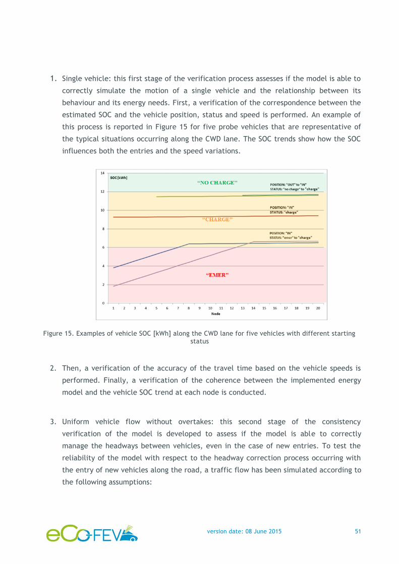
1. Single vehicle: this first stage of the verification process assesses if the model is able to

correctly simulate the motion of a single vehicle and the relationship between its

behaviour and its energy needs. First, a verification of the correspondence between the

estimated SOC and the vehicle position, status and speed is performed. An example of

this process is reported in Figure 15 for five probe vehicles that are representative of

the typical situations occurring along the CWD lane. The SOC trends show how the SOC

influences both the entries and the speed variations.

Figure 15. Examples of vehicle SOC [kWh] along the CWD lane for five vehicles with different starting status

2. Then, a verification of the accuracy of the travel time based on the vehicle speeds is

performed. Finally, a verification of the coherence between the implemented energy

model and the vehicle SOC trend at each node is conducted.

3. Uniform vehicle flow without overtakes: this second stage of the consistency

verification of the model is developed to assess if the model is able to correctly

manage the headways between vehicles, even in the case of new entries. To test the

reliability of the model with respect to the headway correction process occurring with

the entry of new vehicles along the road, a traffic flow has been simulated according to

the following assumptions:


a. identical speeds for “charge” and “emer” vehicles;

b. an average initial traffic headway shorter than the minimum technical headway

allowed in the CWD lane;

c. consequently, the interactions between vehicles are only related to the initial

traffic headway and to new vehicle entries. All headways between vehicles in

the CWD lane must be greater than the minimum technical headway.

4. Complex traffic interaction with overtaking manoeuvres: finally, the third stage aims to

assess the global interaction between vehicles, introducing overtaking manoeuvres. The

model has been tested in a scenario in which overtaking manoeuvres are feasible after

removing the previous simplified assumption 2.a. The number of overtaking manoeuvres

per section, the identification of the vehicles that are overtaking on the nodes, the

time required for the manoeuvres and its influence on the SOC trend because of the

missed recharge have been verified. In the third stage of the model verification

process, traffic results may be controlled by the following relevant parameters

affecting traffic behaviour:

− Input Traffic distribution (average headway, standard deviation and minimum

value);

− Vehicle Speed for the two CWD classes (in the CWD lane where the speed is

controlled and in the other lanes where the speed is derived from the density-speed

relationship);

− Overtake Management (duration, event detection, event activation, event recovery

and multiple overtakes);

− Vehicle Energy parameters (initial SOC, target SOC, SOC thresholds and energy

consumption);

− CWD parameters (system layout and power).

At this stage of the model development, the presented model has been validated by checking

the satisfaction of the established technical requirements, based on the System Engineering

approach (INCOSE, 2011). The main functional requirements for the model are the following:

1. the model shall estimate the number of vehicles in the CWD for any detection point;

2. the model shall consider possible random effects of input flow;

3. the model shall represent the traffic flow at any detection point and reveal if

concentration of traffic and congestion occur along the lane;


4. the model shall take into account different values of the minimum headway allowed in

the CWD to estimate possible effects on traffic and energy for the various CZs over

time.

In the following chapters, the model testing results are reported in an “ideal case”, in which

all of the subsystems and applications involved, such as the CWD booking and authorisation

functions, or the cooperative ADAS, which enables the vehicle cruise control or the

cooperative overtaking, work properly. In this scenario, all related system information, such as

the vehicle position and its SOC, is accurately known. This validation approach could be

considered as a “best-case” testing and it is consistent with the test-case-design methods

applied to test software, such as boundary value analysis (Myers et al., 2004) or distributed

real time systems (Gutiérrez et al., 1998).

2.3.3. Main results of simulated scenarios

After defining the CWD model, it is necessary to estimate its capability to determine the

quality level assessment for the charging service. The electrical power distribution type that

should be supplied at each node is an interesting result from this preliminary stage of CWD

development. The traffic and energy results will be reported in the following sections, where

operational testing scenarios will be analysed.

2.3.3.1. Data setting for the simulated scenarios

The Reference scenario represents a compatible flow of vehicles similar to light vans. Input

traffic flow for the motorway has been simulated according to a hourly time profile along the

day (Figure 3). The variation is described as percentage of the mean value of traffic.

To generalise the simulation for various traffic levels, the traffic parameter chosen is the

traffic density (k), from which the space-mean speed (v) can be estimated, if not observed, by

an empirical model.

The traffic flow (q) for any time interval can be calculated as the product q = k*v*nl (to take

into account the presence on more lanes (nl) for motorways).

The FEVs are only a part of the whole traffic on the motorway and their input traffic has been

estimated as a percentage value, according to the input data assumed in the business model

scenario. FEV arrivals at entrance are then random sampled by an exponential distribution

with the proper average for each time interval according to traffic profile; when the traffic is


low (less than 12 veh/h) the vehicle arrivals are uniformly distributed in the time interval.

Starting form a Reference scenario, also a High Traffic Level and a Low FEV traffic scenario

have been defined, changing, respectively, the average density and the percentage of FEV, as

shown in Table 3.

A further scenario (Alternative) will be explored to analyse how the system performance could

be affected by the minimum allowed technical headway in the CWD lane. In the Alternative

scenario, vehicles are generated closer than those in the Reference scenario, for the higher

traffic level, but they cannot stay too close while charging, thus creating a delay phenomenon

with vehicle platoons in queue. A critical density value of 30 veh/km/lane has been assumed

based on the generally adopted values for freeways under basic conditions (Daganzo, 1997)

[19]. Minimum headway values between 1.5 and 2.5 s have been chosen to consider the use of

ADAS (Yannis, 2004)[23] . Although some car manufacturers use the currently available

adaptive cruise control (ACC) to give the drivers the opportunity to manually choose the

minimal headway, they set the absolute minimum headway at 0.9 s (Hegeman, 2005) [24]. In

this study, a more prudent value of 1.0 s has been assumed.

According to the analysis reported in a previous study (Deflorio et al., 2013)[10], a vehicle

with a SOC less than 30% of its target is assumed in an emergency situation (state = “emer”)

and its desired speed along the CWD lane is set to 30 km/h; if the charging level is between

30% and 60% of the target value, then the vehicle is assumed to be charged in the CWD lane to

preserve its SOC (state =“charge”) and its desired speed is set to 60 km/h. Vehicles with a

current charge level greater than 60% of the target SOC are assumed “out” of the CWD lane

because they do not need to recharge. Their speed is then set according to the feasible speed

in the other lanes, which depend on the estimated traffic density.

Table 3. Different FEVs scenarios

ID SCENARIOS Average density

[Veh/km/lane]

Minimum headway

on CWD [s]

% of FEV Total Traffic

[veh/day]

REF Base (reference) 5 1 10 26086

HTL High Traffic Level 10

1 10 46380

LFT Low FEV Traffic 5 1 1 26086

ALT Alternative 10 3 10 46380


2.3.3.2. Primary traffic and energy results

In this section, a comparison of selected principal traffic results for simulated scenarios is

reported. Because all results depend on the random variables generated at the initial traffic

and energy states, multiple replications of this experiment should be examined to observe,

using statistical analysis, how the random effects influence the simulation results. However, to

better show the traffic and energy behaviour of the implemented simulation model, through

the reading of the calculated variables in identical conditions, the following the results will

focus on one selected replication that is close to the average value.

The first parameter analysed is the FEV traffic flow in the CWD lane. The minimum technical

headway set in the Reference scenario hypothesis (1 s) defines a maximum ideal flow in the

CWD lane of 3600 veh/h. As shown in Figure 16 the Reference scenario traffic flow in the CWD

lane has different time profiles along the lane, with concentration phenomena at the exit

section, although never reaching the ideal value of 3600 veh/h. In particular, based on the

values set for the parameters, an “emer” vehicle increases its SOC and, after reaching the SOC

threshold, it increases its speed according to the “charge” vehicles desired speed, whereas a

“charge” vehicle maintains a constant SOC over time. Consequently, no vehicle leaves the

CWD lane, whereas “out” vehicles can enter into the CWD lane during the simulation (Figure

18 ,Figure 19).

Figure 16. Traffic of FEVs on CWD charging lane during the day at entrance section (node 0) end exit section (node 20) in Reference scenario (REF)

0

50

100

150

200

250

0 1 2 3 4 5 6 7 8 9 10 11 12 13 14 15 16 17 18 19 20 21 22 23 24

FEVs/h

Time [h]

node 0

node 20


Figure 17. Traffic of FEVs on CWD charging lane during the day at entrance section (node 0) end exit section (node 20) in HTL scenario

Figure 18. Traffic of FEVs on CWD charging lane during the day at entrance section (node 0) end exit section (node 20) in LFT Scenario

0

50

100

150

200

250

300

350

400

0 1 2 3 4 5 6 7 8 9 10 11 12 13 14 15 16 17 18 19 20 21 22 23 24

FEVs/h

Time [h]

node 0

node 20

0

5

10

15

20

25

30

0 1 2 3 4 5 6 7 8 9 10 11 12 13 14 15 16 17 18 19 20 21 22 23 24

FEVs/h

Time [h]

node 0

node 20


Figure 19. Traffic of FEVs on CWD charging lane during the day at entrance section (node 0) end exit section (node 20) Alternative scenario (ALT)

Traffic hourly profile along the CWD lane is different from input traffic, due mainly to SOC

variation along the route. An example of the detailed traffic counting along the CWD lane is

reported in Table 4 for the ALT scenario, where the daily profile variation is clearly

represented along the road.

0

50

100

150

200

250

300

350

400

0 1 2 3 4 5 6 7 8 9 10 11 12 13 14 15 16 17 18 19 20 21 22 23 24

FEVs/h

Time [h]

node 0

node 20


Table 4. ALT scenario: traffic counting along the CWD lane

To give a complementary view of traffic variation, also the average headway [s] on the CWD

lane is reported in Table 5 over time and space.

Table 5. ALT scenario: average headway on the CWD lane

Count on CWD h

node 0 1 2 3 4 5 6 7 8 9 10 11 12 13 14 15 16 17 18 19 20 21 22 23 24 Total

1 27 15 11 15 35 84 180 240 245 223 215 217 219 220 212 234 260 273 209 146 106 84 60 34 3564

2 28 18 12 17 37 89 184 255 258 237 230 233 233 233 225 245 271 286 225 155 116 88 64 37 3776

3 30 22 13 18 40 92 195 267 275 251 242 243 242 245 243 256 290 296 233 164 120 91 68 41 3977

4 30 23 15 19 42 96 201 274 287 262 251 250 255 257 255 268 303 307 245 172 129 97 71 43 1 4153

5 30 23 16 19 43 98 212 287 300 269 260 257 262 264 265 278 308 315 256 179 135 102 75 44 1 4298

6 30 24 16 20 43 102 216 295 307 276 269 269 271 267 277 284 315 323 262 185 139 105 79 44 1 4419

7 30 25 16 20 43 105 218 296 325 283 275 274 276 273 287 289 324 328 272 193 140 108 80 46 2 4528

8 30 26 16 20 43 106 219 301 334 288 278 280 280 274 292 292 326 332 280 195 140 109 82 47 2 4592

9 30 26 17 21 43 107 226 295 348 290 282 285 280 279 294 292 331 337 280 197 140 111 83 48 2 4644

10 30 26 18 21 44 104 231 300 356 294 282 289 284 280 294 296 334 343 287 197 142 110 85 49 2 4698

11 31 26 18 20 44 104 231 296 361 298 284 292 286 287 288 299 337 349 286 199 143 107 89 48 3 4726

12 29 28 18 21 44 102 232 295 359 306 281 297 286 292 282 304 343 349 289 203 146 106 90 47 4 4753

13 28 29 17 22 43 101 228 300 356 312 277 302 281 297 278 306 345 349 292 206 150 104 90 47 6 4766

14 28 29 17 21 41 101 228 299 357 316 274 304 282 297 279 304 347 347 295 207 152 104 88 51 6 4774

15 28 29 17 20 42 99 227 300 357 315 269 309 278 301 280 299 352 347 295 209 152 106 88 49 9 4777

16 28 29 16 21 41 98 227 294 356 316 273 312 271 304 280 295 351 352 296 211 154 108 86 51 9 4779

17 27 30 16 20 42 96 220 298 356 316 274 308 275 304 273 304 343 355 295 212 156 108 90 51 10 4779

18 26 31 16 20 42 94 216 299 355 316 276 310 274 300 275 303 344 350 300 214 158 108 89 52 11 4779

19 26 31 16 20 42 92 215 296 355 315 277 307 276 301 276 304 343 344 308 209 164 107 91 52 12 4779

20 24 33 16 20 42 91 213 292 353 317 275 310 275 302 278 302 343 344 305 212 168 106 92 54 12 4779

Total 570 523 317 395 836 1961 4319 5779 6600 5800 5344 5648 5386 5577 5433 5754 6510 6626 5510 3865 2850 2069 1640 935 93 90340

Mean of HeadWay[s] h

node 0 1 2 3 4 5 6 7 8 9 10 11 12 13 14 15 16 17 18 19 20 21 22 23 24 Total

1 120 143 397 257 100 45 20 16 14 15 17 16 17 16 18 15 14 13 17 25 34 45 55 115 24

2 117 116 369 223 94 43 19 15 13 14 16 15 16 15 16 15 14 12 16 23 32 43 51 108 23

3 100 110 343 207 88 42 18 15 12 14 15 15 15 15 15 14 13 12 15 22 31 41 48 98 22

4 102 102 297 196 85 41 18 13 12 13 14 15 14 14 14 14 12 12 14 21 29 38 45 88 293 21

5 104 100 279 196 83 38 18 13 12 13 14 14 14 14 13 14 12 11 13 21 28 35 44 88 293 20

6 92 111 279 187 83 36 17 13 11 13 13 13 14 13 12 13 11 11 13 20 27 34 42 89 293 19

7 92 106 279 187 83 35 17 12 11 13 13 13 13 13 13 13 11 11 13 19 26 33 42 80 258 19

8 92 102 279 187 83 35 16 12 10 13 13 13 13 13 12 13 11 11 13 19 26 33 42 79 258 19

9 92 102 262 178 83 35 16 12 10 12 13 13 13 13 12 13 11 11 13 19 24 35 41 77 258 19

10 92 102 248 178 81 35 16 12 10 12 13 12 13 12 13 12 11 10 13 18 24 34 41 76 258 18

11 89 102 248 175 84 35 16 12 10 12 13 12 13 12 13 12 11 10 13 18 24 35 40 76 188 18

12 93 97 248 167 84 35 16 12 10 12 13 12 13 12 13 12 11 10 12 18 24 35 40 76 156 18

13 86 104 253 166 85 36 16 12 10 12 13 12 13 12 13 12 10 10 12 18 24 34 40 75 128 18

14 86 104 253 172 87 36 16 12 10 11 13 12 13 12 13 12 10 10 12 17 24 34 41 70 128 18

15 86 104 253 175 87 36 16 12 10 11 13 12 13 12 13 12 10 10 12 17 24 33 41 72 99 18

16 86 104 249 182 82 39 16 12 10 11 13 12 13 12 13 12 10 10 12 17 23 33 42 70 99 18

17 88 101 249 177 87 39 17 12 10 11 13 12 13 12 13 12 10 10 12 17 23 33 40 71 92 18

18 87 102 249 177 87 39 17 12 10 11 13 12 13 12 13 12 10 10 12 17 23 34 40 70 90 18

19 87 102 249 177 87 40 17 12 10 11 13 12 13 12 13 12 11 10 12 17 22 34 40 68 92 18

20 92 97 249 177 87 40 17 12 10 11 13 12 13 12 13 12 10 10 12 17 21 34 39 67 92 18

Total 94 104 272 186 86 38 17 13 11 12 14 13 13 13 13 13 11 11 13 19 25 35 42 79 124 19


For the same scenario (ALT) a more detailed representation during the peak hour period within

the 15h – 18h is reported in Table 6 for a higher time resolution (5 minutes).

Table 6. ALT scenario: traffic counting along the CWD lane during the peak hour period (15h-18h) with 5 minutes resolution

From this figure, FEVs distribution along the motorway shows some concentration phenomena

due to random arrival and SOC variations. However, the delay for charging vehicles, which is

concentrated in the first part of the motorway, is not relevant because, the maximum value

detected during simulation is 7s, as shown in Table 7.

Table 7. ALT scenario: maximum delay for charging vehicles

Count on CWD h

180 181 182 183 184 185 186 187 188 189 190 191 192 193 194 195 196 197 198 199 200 201 202 203 204 205 206 207 208 209 210 211 212 213 214 215 216 217 218 219 220 221 222 223 224 225 226 227

node 15 15 15 15 15 15 15 15 15 15 15 15 16 16 16 16 16 16 16 16 16 16 16 16 17 17 17 17 17 17 17 17 17 17 17 17 18 18 18 18 18 18 18 18 18 18 18 18

1 13 23 25 24 23 23 18 25 19 36 5 36 22 25 25 18 21 23 30 24 31 5 22 31 25 27 22 25 26 32 33 29 1 14 27 20 16 21 25 21 23 21 21

2 10 23 23 28 24 26 20 26 18 31 16 31 26 22 25 20 21 23 33 24 34 12 12 33 29 27 24 27 26 37 33 26 12 12 28 23 15 20 32 22 22 22 23 6

3 7 21 27 28 25 31 16 26 19 32 24 17 33 28 25 24 23 25 35 28 32 19 1 8 33 27 32 27 28 22 39 30 33 17 4 28 28 19 19 30 24 23 25 20 13

4 4 16 31 27 27 33 22 24 25 28 28 3 10 34 29 28 28 23 26 35 31 32 25 2 6 28 36 29 29 31 18 43 27 37 20 3 4 24 28 24 20 25 30 24 26 24 16

5 17 28 27 29 36 27 22 25 25 37 5 42 25 32 28 24 25 33 34 32 29 4 27 39 28 31 31 26 35 30 38 26 4 2 23 26 24 25 22 32 29 21 31 21

6 14 25 26 32 31 32 18 34 21 40 11 39 24 32 30 23 27 34 33 32 31 10 1 20 38 30 34 30 29 29 40 33 36 3 1 20 27 28 20 25 35 25 25 28 26 2

7 12 25 25 29 33 33 24 32 23 32 21 2 32 29 29 29 26 31 25 39 29 37 16 1 15 34 37 33 29 31 27 44 32 34 11 1 16 28 29 24 22 38 25 25 25 32 7

8 9 21 30 27 32 34 26 28 26 32 27 2 20 34 31 31 30 23 31 37 31 36 20 3 11 33 37 31 33 33 21 41 37 35 17 3 7 31 31 28 22 36 28 24 26 30 14

9 6 18 33 28 28 36 27 26 32 29 29 6 12 37 30 32 33 24 29 37 33 35 23 4 9 28 40 31 34 35 21 42 31 37 25 2 7 26 27 32 22 32 33 25 27 27 20

10 2 2 18 30 31 28 38 30 24 31 26 36 7 2 44 28 34 33 27 28 33 38 35 25 8 3 28 40 29 34 36 27 35 34 40 29 3 4 27 27 29 29 26 37 27 23 30 25

11 8 2 15 27 30 30 35 31 22 36 21 42 11 2 40 27 33 33 26 30 33 36 33 33 11 3 21 37 33 36 32 31 30 41 38 36 3 23 31 32 25 26 40 25 25 28 28

12 17 15 26 29 31 34 32 27 34 25 34 21 2 33 32 28 34 27 33 26 40 29 38 15 2 16 34 39 33 33 33 29 44 36 35 11 18 30 31 27 23 42 25 26 26 30

13 23 1 12 21 31 32 32 35 27 31 27 34 26 3 20 36 32 31 33 27 31 38 31 37 19 4 11 33 37 35 35 35 22 44 37 37 17 2 9 31 33 30 23 36 30 26 26 29

14 26 1 7 18 33 33 29 37 27 28 33 32 28 7 12 37 32 32 36 27 30 37 33 36 24 4 9 28 41 34 35 36 22 42 32 40 25 2 8 26 29 34 23 32 35 26 28 27

15 29 3 3 18 30 32 30 38 29 27 32 28 36 7 2 44 29 35 33 29 30 33 37 37 25 8 3 28 40 31 36 36 29 35 35 41 29 3 3 28 27 30 29 26 37 29 23 31

16 29 9 2 16 27 31 32 35 31 23 38 22 42 11 2 40 28 33 33 28 31 33 36 34 33 11 3 21 37 35 38 33 32 30 41 38 36 3 23 31 32 25 26 40 26 26 28

17 32 17 15 26 29 32 34 32 27 35 25 34 21 2 33 32 29 34 28 34 26 40 30 38 15 2 16 34 40 34 34 33 29 44 36 35 11 18 30 31 27 23 42 26 26 26

18 30 23 1 12 21 31 32 32 35 27 32 27 34 26 3 20 36 33 31 33 28 31 38 31 37 19 4 11 33 37 35 35 36 22 44 37 37 17 2 9 31 33 30 23 36 30 26 26

19 32 26 1 7 18 33 33 29 37 27 28 33 32 28 7 12 37 32 32 36 27 30 37 33 36 24 4 9 28 41 34 35 37 22 42 32 40 25 2 8 26 29 34 23 32 35 26 28

20 31 29 3 3 18 30 32 30 38 29 27 32 28 36 7 2 44 29 35 33 29 30 33 37 37 25 8 3 28 40 31 36 37 29 35 35 41 29 3 3 28 27 30 29 26 37 29 23

Max di Delay h

node 0 1 2 3 4 5 6 7 8 9 10 11 12 13 14 15 16 17 18 19 20 21 22 23 24 Total

1 0.0 0.0 0.0 0.0 1.0 0.0 6.0 3.0 3.0 3.0 3.0 3.0 3.0 3.0 2.0 3.0 3.0 3.0 3.0 3.0 0.0 0.0 0.0 0.0 6.0

2 0.0 0.0 0.0 0.0 0.0 2.0 3.0 3.0 5.0 6.0 3.0 3.0 5.0 3.0 3.0 3.0 6.0 3.0 3.0 3.0 2.0 3.0 0.0 0.0 6.0

3 2.0 0.0 0.0 0.0 2.0 3.0 3.0 3.0 4.0 4.0 3.0 3.0 3.0 3.0 3.0 4.0 3.0 5.0 3.0 3.0 3.0 3.0 0.0 0.0 5.0

4 0.0 0.0 0.0 0.0 1.0 2.0 3.0 4.0 3.0 4.0 3.0 5.0 5.0 3.0 3.0 4.0 3.0 7.0 5.0 3.0 3.0 3.0 0.0 1.0 0.0 7.0

5 0.0 0.0 0.0 0.0 1.0 1.0 3.0 5.0 4.0 3.0 3.0 3.0 6.0 3.0 3.0 3.0 3.0 3.0 4.0 3.0 2.0 3.0 0.0 0.0 0.0 6.0

6 0.0 1.0 0.0 0.0 0.0 0.0 3.0 3.0 3.0 3.0 3.0 3.0 3.0 4.0 3.0 6.0 3.0 3.0 3.0 2.0 3.0 1.0 0.0 0.0 0.0 6.0

7 0.0 3.0 0.0 0.0 0.0 3.0 3.0 3.0 3.0 3.0 3.0 2.0 3.0 3.0 3.0 3.0 3.0 3.0 3.0 3.0 2.0 2.0 0.0 0.0 0.0 3.0

8 0.0 0.0 0.0 0.0 2.0 1.0 3.0 3.0 4.0 3.0 3.0 2.0 3.0 3.0 2.0 3.0 3.0 3.0 3.0 3.0 0.0 0.0 0.0 0.0 0.0 4.0

9 0.0 0.0 0.0 0.0 0.0 2.0 3.0 2.0 3.0 3.0 3.0 1.0 2.0 3.0 2.0 2.0 3.0 3.0 3.0 3.0 0.0 0.0 0.0 1.0 0.0 3.0

10 0.0 0.0 0.0 0.0 0.0 0.0 3.0 6.0 3.0 0.0 2.0 3.0 3.0 3.0 3.0 3.0 2.0 3.0 3.0 1.0 3.0 3.0 0.0 0.0 0.0 6.0

11 0.0 0.0 0.0 0.0 0.0 1.0 3.0 0.0 3.0 1.0 3.0 2.0 3.0 3.0 3.0 2.0 3.0 3.0 3.0 1.0 0.0 3.0 0.0 0.0 0.0 3.0

12 0.0 0.0 0.0 0.0 0.0 0.0 2.0 2.0 0.0 3.0 1.0 0.0 2.0 2.0 3.0 3.0 3.0 3.0 2.0 3.0 0.0 0.0 0.0 0.0 0.0 3.0

13 0.0 0.0 0.0 0.0 0.0 0.0 2.0 2.0 3.0 0.0 2.0 0.0 2.0 1.0 0.0 0.0 1.0 1.0 0.0 2.0 0.0 0.0 0.0 0.0 0.0 3.0

14 0.0 0.0 0.0 0.0 0.0 0.0 0.0 0.0 0.0 3.0 0.0 0.0 3.0 3.0 0.0 1.0 0.0 0.0 0.0 0.0 1.0 0.0 0.0 0.0 0.0 3.0

15 0.0 0.0 0.0 0.0 0.0 0.0 0.0 0.0 0.0 0.0 0.0 0.0 3.0 0.0 0.0 0.0 0.0 0.0 0.0 0.0 0.0 0.0 0.0 0.0 0.0 3.0

16 0.0 0.0 0.0 0.0 0.0 0.0 0.0 0.0 0.0 0.0 0.0 0.0 0.0 0.0 0.0 0.0 0.0 3.0 0.0 0.0 0.0 0.0 0.0 0.0 0.0 3.0

17 0.0 0.0 0.0 0.0 0.0 0.0 0.0 0.0 0.0 0.0 0.0 0.0 0.0 0.0 0.0 0.0 0.0 0.0 0.0 0.0 0.0 0.0 0.0 0.0 0.0 0.0

18 0.0 0.0 0.0 0.0 0.0 0.0 0.0 0.0 0.0 0.0 0.0 0.0 0.0 0.0 0.0 0.0 0.0 0.0 0.0 0.0 0.0 0.0 0.0 0.0 0.0 0.0

19 0.0 0.0 0.0 0.0 0.0 0.0 0.0 0.0 0.0 0.0 0.0 0.0 0.0 0.0 0.0 0.0 0.0 0.0 0.0 0.0 0.0 0.0 0.0 0.0 0.0 0.0

20 0.0 0.0 0.0 0.0 0.0 0.0 0.0 0.0 0.0 0.0 0.0 0.0 0.0 0.0 0.0 0.0 0.0 0.0 0.0 0.0 0.0 0.0 0.0 0.0 0.0 0.0

Total 2.0 3.0 0.0 0.0 2.0 3.0 6.0 6.0 5.0 6.0 3.0 5.0 6.0 4.0 3.0 6.0 6.0 7.0 5.0 3.0 3.0 3.0 0.0 1.0 0.0 7.0


As for the OUT vehicles, their speed during the day (Table 8) follows the trend assumed for the

traffic profile and the speed-density relationship assumed.

Table 8. ALT scenario: speed during the day for the OUT vehicles

The effect of CWD on SOC for vehicle is shown in Table 9 where average values of the various

vehicles are reported.

Table 9. ALT scenario: effect of the CWD on the vehicles average SOC

AvSpeed [km/h] (OUT) h

node 0 1 2 3 4 5 6 7 8 9 10 11 12 13 14 15 16 17 18 19 20 21 22 23 Total

1 110 110 110 110 110 108 102 92 91 97 98 97 97 97 96 95 90 89 98 105 107 108 109 110 110

2 110 110 110 110 110 108 102 92 91 97 98 97 97 97 96 95 90 89 98 105 107 108 109 110 110

3 110 110 110 110 110 108 102 92 91 97 98 97 97 97 96 95 90 89 98 105 107 108 109 110 110

4 110 110 110 110 110 108 102 92 91 97 98 97 97 97 96 95 90 89 98 105 107 108 109 110 110

5 110 110 110 110 110 108 102 92 91 97 98 97 97 97 96 95 90 89 98 105 107 108 109 110 110

6 110 110 110 110 110 108 102 92 91 97 98 97 97 97 96 95 90 89 98 105 107 108 109 110 110

7 110 110 110 110 110 108 102 92 91 97 98 97 97 97 96 95 90 89 98 105 107 108 109 110 110

8 110 110 110 110 108 102 92 91 97 98 97 97 97 96 95 90 89 98 105 107 108 109 110 110

9 110 110 110 110 102 92 91 97 98 97 97 97 96 95 90 89 98 105 108 109 110 110

10 110 110 102 92 91 97 98 97 97 97 96 95 90 89 98 105 109 110

11 110 102 92 91 97 98 97 97 97 96 95 90 89 98 105 110

12 102 92 91 97 97 97 95 90 89 98 105 105

13 92 91 97 95 90 89 97

14 92 91 97 89 97

15 91 89 91

Total 110 110 110 110 110 108 102 92 91 97 98 97 97 97 96 95 90 89 98 105 107 108 109 110 110

Mean of SoC [kWh] h

node 0 1 2 3 4 5 6 7 8 9 10 11 12 13 14 15 16 17 18 19 20 21 22 23 24 Total

1 8.0 8.4 9.2 8.5 8.2 8.6 8.5 8.3 8.4 8.6 8.6 8.4 8.5 8.4 8.6 8.5 8.3 8.6 8.3 8.6 8.2 8.5 9.0 8.1 8.5

2 8.1 8.9 9.4 8.8 8.4 8.8 8.6 8.5 8.6 8.8 8.8 8.7 8.7 8.6 8.8 8.7 8.4 8.8 8.6 8.8 8.5 8.7 9.2 8.4 8.7

3 8.4 9.4 9.6 9.0 8.7 8.9 8.8 8.7 8.8 8.9 9.0 8.8 8.8 8.7 9.0 8.8 8.7 8.9 8.7 9.0 8.6 8.8 9.3 8.7 8.8

4 8.5 9.5 9.8 9.1 8.9 9.0 8.9 8.8 8.9 9.1 9.1 8.9 9.0 8.9 9.2 9.0 8.8 9.0 8.9 9.1 8.8 9.0 9.4 9.0 5.9 9.0

5 8.5 9.5 9.9 9.1 9.0 9.2 9.0 9.0 9.0 9.2 9.2 9.0 9.1 9.0 9.3 9.1 8.9 9.1 9.0 9.3 9.0 9.2 9.4 9.1 6.2 9.1

6 8.8 9.3 9.9 9.3 9.1 9.3 9.1 9.0 9.1 9.2 9.3 9.1 9.2 9.0 9.4 9.1 9.0 9.2 9.0 9.3 9.1 9.3 9.5 9.1 6.6 9.2

7 8.8 9.4 9.9 9.3 9.1 9.4 9.2 9.2 9.2 9.3 9.3 9.2 9.3 9.1 9.5 9.2 9.0 9.2 9.1 9.4 9.2 9.3 9.5 9.3 6.6 9.2

8 8.8 9.5 9.9 9.3 9.1 9.4 9.2 9.2 9.3 9.3 9.4 9.2 9.3 9.1 9.5 9.3 9.1 9.3 9.2 9.5 9.2 9.3 9.5 9.4 6.6 9.3

9 8.8 9.5 10.0 9.4 9.1 9.5 9.3 9.3 9.3 9.4 9.4 9.2 9.3 9.2 9.5 9.3 9.1 9.3 9.2 9.5 9.3 9.3 9.6 9.4 6.6 9.3

10 8.9 9.6 10.1 9.4 9.2 9.5 9.3 9.3 9.3 9.4 9.5 9.3 9.3 9.2 9.5 9.4 9.1 9.3 9.2 9.6 9.2 9.3 9.6 9.5 6.6 9.3

11 8.9 9.6 10.1 9.4 9.3 9.5 9.4 9.4 9.3 9.4 9.5 9.3 9.4 9.3 9.6 9.4 9.2 9.3 9.3 9.6 9.2 9.3 9.6 9.5 7.6 9.4

12 8.8 9.7 10.1 9.5 9.3 9.6 9.4 9.4 9.3 9.5 9.5 9.3 9.4 9.3 9.6 9.5 9.2 9.3 9.3 9.6 9.2 9.4 9.6 9.6 7.7 9.4

13 8.9 9.7 10.3 9.4 9.3 9.6 9.4 9.4 9.3 9.5 9.5 9.3 9.4 9.3 9.6 9.5 9.3 9.3 9.3 9.6 9.2 9.4 9.6 9.6 7.7 9.4

14 8.9 9.7 10.3 9.3 9.4 9.6 9.4 9.4 9.3 9.5 9.5 9.4 9.5 9.3 9.6 9.5 9.3 9.3 9.4 9.6 9.3 9.4 9.7 9.6 7.7 9.4

15 8.9 9.7 10.3 9.2 9.5 9.6 9.5 9.4 9.3 9.5 9.5 9.4 9.5 9.3 9.7 9.5 9.3 9.3 9.3 9.6 9.3 9.5 9.7 9.6 8.4 9.4

16 8.9 9.7 10.4 9.2 9.6 9.6 9.5 9.5 9.3 9.6 9.5 9.4 9.5 9.3 9.6 9.5 9.3 9.3 9.4 9.6 9.3 9.4 9.7 9.6 8.4 9.5

17 8.8 9.8 10.4 9.3 9.5 9.5 9.5 9.5 9.3 9.6 9.6 9.3 9.6 9.3 9.6 9.5 9.3 9.4 9.4 9.6 9.3 9.4 9.8 9.6 8.2 9.5

18 8.8 9.8 10.4 9.3 9.5 9.6 9.5 9.5 9.3 9.6 9.6 9.3 9.6 9.3 9.7 9.6 9.3 9.4 9.4 9.6 9.3 9.5 9.7 9.6 8.5 9.5

19 8.8 9.8 10.5 9.4 9.5 9.6 9.5 9.6 9.3 9.7 9.6 9.3 9.6 9.3 9.7 9.6 9.3 9.4 9.4 9.6 9.3 9.5 9.8 9.5 8.8 9.5

20 8.7 9.8 10.5 9.4 9.5 9.6 9.5 9.6 9.3 9.6 9.6 9.4 9.6 9.3 9.7 9.6 9.3 9.4 9.4 9.6 9.3 9.5 9.8 9.5 8.8 9.5

Total 8.7 9.6 10.1 9.2 9.2 9.4 9.2 9.2 9.2 9.4 9.4 9.2 9.3 9.1 9.5 9.3 9.1 9.2 9.2 9.4 9.1 9.3 9.6 9.3 8.1 9.3


To show the advantage of CWD service for the low-SOC vehicles (in emergency cases) also their

minimum value is reported over time and space (Table 10).

Table 10. ALT scenario: effect of the CWD on the low-SOC vehicles

As relevant output from simulation, also the total energy provided to FEV has been estimated

along the motorway over the whole day for the selected 4 scenarios. Results for the simulated

scenarios are reported in Table 11, Table 12, Table 13 and Table 14.

Table 11. Energy received by FEVs between nodes during the 24 hour of the day in the Reference scenario

Min of SoC [kWh] h

node 0 1 2 3 4 5 6 7 8 9 10 11 12 13 14 15 16 17 18 19 20 21 22 23 24 Total

1 2.2 4.5 5.8 4.4 3.1 2.6 1.8 1.8 1.8 1.8 1.8 2.9 1.8 1.8 1.8 2.7 2.4 2.5 2.5 2.2 1.8 2.0 4.4 4.7 1.8

2 2.5 4.9 6.2 4.8 3.5 2.9 2.2 2.2 2.2 2.2 2.2 3.3 2.2 2.2 2.2 3.1 2.8 2.9 2.9 2.6 2.2 2.4 4.7 5.1 2.2

3 2.9 5.2 6.5 5.2 3.8 3.3 2.6 2.6 2.6 2.6 2.6 3.6 2.6 2.6 2.6 3.4 3.1 3.3 3.2 3.0 2.6 2.8 5.1 5.4 2.6

4 3.3 5.6 6.5 5.5 4.2 3.7 2.9 2.9 2.9 2.9 2.9 4.0 2.9 2.9 2.9 3.8 3.5 3.6 3.6 3.3 2.9 3.1 5.5 5.8 5.9 2.9

5 3.6 6.0 6.6 5.9 4.6 4.0 3.3 3.3 3.3 3.3 3.3 4.4 3.3 3.3 3.3 4.2 3.9 4.0 4.0 3.7 3.3 3.5 5.7 6.2 6.2 3.3

6 4.4 4.0 6.6 6.2 4.9 4.4 3.7 3.7 3.7 3.7 3.7 4.7 3.7 3.7 3.7 4.6 4.2 4.4 4.3 4.1 3.7 3.9 6.0 6.2 6.6 3.7

7 4.8 4.4 6.6 6.2 5.3 4.8 4.0 4.0 4.1 4.0 4.0 5.1 4.0 4.0 4.0 4.9 4.6 4.7 4.7 4.4 4.0 4.2 6.2 6.2 6.6 4.0

8 5.2 4.7 6.6 6.2 5.7 5.1 4.4 4.4 4.4 4.4 4.4 4.4 4.4 4.4 4.4 5.3 5.0 5.1 5.1 4.8 4.4 4.6 6.3 6.2 6.6 4.4

9 5.5 5.1 6.6 6.2 6.0 5.5 4.8 4.8 4.8 4.8 4.8 4.8 4.8 4.8 4.8 5.7 5.4 5.5 5.4 5.2 4.8 5.0 6.3 6.2 6.6 4.8

10 5.9 5.5 6.6 6.2 6.2 5.9 5.2 5.1 5.2 5.1 5.1 5.1 5.1 5.1 5.1 5.7 5.7 5.8 5.8 5.5 5.1 5.3 6.3 6.3 6.6 5.1

11 6.1 5.8 6.6 6.2 6.2 6.2 5.5 5.5 5.5 5.5 5.5 5.5 5.5 5.5 5.5 6.1 6.1 6.1 6.0 5.9 5.5 5.7 6.3 6.3 6.6 5.5

12 6.2 6.2 6.6 6.3 6.2 6.2 5.9 5.9 5.9 5.9 5.9 5.9 5.9 5.9 5.9 6.0 6.1 6.1 6.1 6.3 5.9 6.1 6.3 6.3 6.7 5.9

13 6.2 6.6 7.4 6.3 6.2 6.2 6.3 6.1 6.2 6.1 6.1 6.1 6.1 6.1 6.2 6.2 6.1 6.1 6.1 6.4 6.1 6.4 6.3 6.3 6.5 6.1

14 6.2 6.6 7.4 6.3 6.2 6.2 6.3 6.1 6.2 6.2 6.1 6.1 6.1 6.1 6.2 6.2 6.1 6.1 6.1 6.4 6.1 6.4 6.3 6.3 6.5 6.1

15 6.2 6.6 7.4 6.3 6.2 6.2 6.3 6.1 6.2 6.2 6.1 6.1 6.1 6.1 6.3 6.2 6.1 6.1 6.1 6.4 6.1 6.4 6.3 6.3 6.5 6.1

16 6.2 6.6 7.4 6.3 6.2 6.2 6.3 6.1 6.3 6.2 6.1 6.1 6.1 6.2 6.3 6.2 6.1 6.1 6.1 6.4 6.1 6.4 6.3 6.3 6.5 6.1

17 6.2 6.6 7.4 6.3 6.2 6.3 6.3 6.1 6.3 6.2 6.1 6.1 6.1 6.2 6.3 6.2 6.1 6.1 6.1 6.5 6.1 6.4 6.4 6.6 6.3 6.1

18 6.2 6.6 7.4 6.3 6.3 6.3 6.3 6.1 6.3 6.2 6.1 6.1 6.1 6.2 6.3 6.2 6.1 6.1 6.1 6.5 6.1 6.4 6.4 6.6 6.3 6.1

19 6.2 6.6 7.4 6.3 6.3 6.3 6.3 6.2 6.1 6.2 6.1 6.2 6.1 6.2 6.3 6.2 6.1 6.1 6.1 6.5 6.1 6.5 6.4 6.6 6.4 6.1

20 6.2 6.6 7.4 6.3 6.3 6.3 6.4 6.2 6.1 6.2 6.1 6.2 6.2 6.2 6.3 6.2 6.1 6.2 6.1 6.4 6.2 6.5 6.4 6.4 6.4 6.1

Total 2.2 4.0 5.8 4.4 3.1 2.6 1.8 1.8 1.8 1.8 1.8 2.9 1.8 1.8 1.8 2.7 2.4 2.5 2.5 2.2 1.8 2.0 4.4 4.7 5.9 1.8

EnPosReceived

InSection[kWh] h

node 0 1 2 3 4 5 6 7 8 9 10 11 12 13 14 15 16 17 18 19 20 21 22 23 24 Total

1 3.8 2.4 2.4 2.2 5.7 13.3 28.1 39.6 42.0 36.9 34.1 32.8 35.6 39.0 37.2 37.8 45.1 40.5 33.1 23.0 15.2 13.8 9.0 6.7 579.2

2 3.8 2.7 2.4 2.2 5.8 13.7 28.6 41.0 42.5 37.6 35.3 33.5 36.9 39.8 38.4 40.0 46.7 42.6 34.9 23.7 16.2 14.1 9.1 6.7 598.1

3 4.1 3.4 2.6 2.4 5.4 15.6 30.0 45.5 44.9 40.1 37.9 36.6 39.5 42.3 41.1 42.2 50.5 46.2 38.0 25.4 17.5 15.4 9.8 6.9 643.2

4 4.5 3.5 2.7 2.7 5.6 16.6 31.7 46.8 47.1 41.0 39.1 38.1 40.0 42.4 41.1 42.7 53.1 48.4 39.7 26.7 19.1 15.9 10.4 6.9 665.7

5 4.0 3.5 2.7 2.8 5.6 17.2 33.4 46.7 49.3 42.7 39.3 37.9 40.1 41.8 41.6 44.2 52.4 50.2 40.8 27.0 19.4 16.0 10.4 7.1 676.1

6 4.0 3.2 3.0 2.4 5.9 16.8 32.8 48.5 50.7 43.7 40.2 39.6 41.4 41.8 42.6 44.2 53.2 51.4 41.2 27.5 19.1 16.0 10.4 7.4 687.1

7 4.0 3.2 2.4 2.7 5.4 16.4 33.4 49.5 51.5 43.4 40.4 41.0 42.7 42.5 42.6 43.6 54.9 53.1 40.5 28.1 19.0 15.8 10.3 7.8 694.1

8 4.2 3.2 2.4 2.7 5.5 16.4 33.4 50.5 51.1 44.4 40.5 41.3 43.5 42.5 43.4 41.7 56.6 53.7 42.0 28.3 19.4 15.8 10.6 7.8 701.0

9 4.3 3.0 2.4 2.7 5.4 16.8 32.9 51.1 50.3 45.2 41.2 40.8 43.6 42.9 43.6 42.0 57.2 54.2 43.7 28.1 19.3 16.2 10.9 7.5 705.2

10 4.0 3.2 2.4 2.8 5.1 16.7 32.9 50.8 50.9 45.2 41.4 40.9 44.5 42.7 44.4 41.0 58.7 54.5 42.7 28.5 18.5 16.9 10.8 7.5 707.2

11 4.0 3.2 2.4 3.0 5.1 16.1 32.1 52.2 50.2 45.7 40.2 41.3 46.1 42.5 44.5 39.5 60.5 54.7 42.5 28.8 17.9 17.4 10.5 7.3 0.5 708.1

12 4.0 3.0 2.7 2.7 5.1 16.2 31.4 53.0 49.7 46.5 39.1 42.5 46.3 41.9 44.9 38.6 61.8 54.6 42.1 29.3 16.7 18.7 10.5 7.0 0.5 709.0

13 3.8 3.2 2.7 2.7 4.8 16.4 30.7 53.0 49.5 46.3 39.3 42.5 47.4 41.1 44.4 39.0 62.4 54.0 42.3 29.3 17.0 18.4 10.2 7.3 0.8 708.6

14 3.8 3.2 2.7 2.7 4.8 15.6 31.2 52.4 48.7 46.3 39.7 43.8 47.9 40.0 43.9 40.4 62.3 53.3 42.0 29.9 17.5 18.6 9.7 7.8 0.8 708.8

15 3.8 3.2 2.4 3.0 4.8 15.1 31.2 52.5 47.6 46.0 40.6 44.1 48.2 38.8 44.4 39.6 61.9 54.1 42.5 28.8 18.6 18.6 9.4 7.8 0.8 707.9

16 3.8 3.2 2.4 3.0 4.8 15.1 31.0 51.4 47.4 47.1 40.1 45.2 47.6 39.0 43.9 38.5 63.5 53.8 42.3 28.8 19.4 18.3 9.7 7.8 0.8 707.9

17 3.8 3.2 2.4 3.0 4.8 14.5 31.2 49.5 49.3 46.0 41.2 45.2 47.1 39.3 42.8 40.1 62.7 53.6 42.5 29.1 19.4 18.8 9.4 7.8 1.1 707.9

18 3.8 3.2 2.4 3.0 4.8 14.5 30.4 49.8 49.8 45.2 41.5 45.2 47.4 39.0 42.0 39.8 62.2 54.9 43.1 28.3 20.2 18.6 9.4 8.3 1.1 707.9

19 3.2 3.8 2.4 3.0 4.8 14.3 30.4 49.0 49.8 45.5 41.5 45.2 47.6 38.5 41.7 40.1 62.2 54.6 43.1 28.5 21.0 18.8 8.9 8.6 1.3 707.9

20 3.2 3.5 2.7 2.7 4.8 14.3 29.6 48.7 50.3 45.8 41.5 44.4 47.4 39.0 42.5 39.8 61.4 54.4 43.3 29.3 20.7 19.4 9.2 8.3 1.6 707.9

Total 77.8 64.2 50.8 54.2 104.3 311.7 626.5 981.4 972.6 880.6 794.1 822.0 880.8 816.8 851.1 814.8 1149.3 1036.9 822.0 556.4 371.0 341.4 198.6 150.2 9.4 13 738.82


Table 12. Energy received by FEVs between nodes during the 24 hour of the day in the HTL Scenario

Table 13. Energy received by FEVs between nodes during the 24 hour of the day in the LFT scenario

EnPosReceived

InSection[kWh] h

node 0 1 2 3 4 5 6 7 8 9 10 11 12 13 14 15 16 17 18 19 20 21 22 23 24 Total

1 8.6 3.8 3.8 3.7 12.3 20.0 49.6 71.3 69.4 62.1 56.2 62.8 64.4 62.6 63.7 68.2 70.1 70.2 57.4 43.4 31.5 26.5 16.9 12.0 1010.3

2 8.8 4.1 4.1 4.2 12.4 22.0 51.8 73.2 71.0 64.2 58.8 62.8 67.2 63.4 66.2 70.9 72.0 73.9 58.6 44.5 32.5 26.5 17.7 12.4 1043.0

3 9.3 4.7 4.5 5.1 13.4 24.7 56.3 77.8 75.7 69.2 63.9 68.5 70.9 68.6 68.1 75.0 75.7 81.3 61.9 48.4 35.0 27.6 19.0 13.8 1118.4

4 9.5 5.2 3.6 5.7 12.7 27.4 58.0 79.0 79.1 72.1 67.5 71.4 72.2 70.6 70.8 77.7 78.9 83.3 65.4 50.4 36.3 28.8 20.1 14.3 1160.1

5 9.8 5.3 4.2 5.7 12.2 28.3 59.3 79.4 80.5 73.5 69.7 72.1 73.7 70.8 72.5 79.6 82.1 83.9 67.7 50.5 36.6 29.5 21.0 14.2 1182.3

6 9.4 5.8 4.2 6.3 12.1 28.9 60.0 81.3 82.3 75.8 71.7 72.6 75.8 70.4 76.6 80.0 81.8 86.8 70.7 50.6 38.3 29.4 21.9 13.6 1206.4

7 9.2 5.4 4.6 6.4 12.1 29.3 59.7 85.3 83.7 76.9 73.4 73.4 77.2 73.3 79.0 80.6 83.7 88.2 73.0 51.9 38.2 29.7 22.1 12.9 0.5 1229.5

8 9.2 5.1 4.8 6.8 11.6 29.5 60.2 85.1 86.4 76.9 74.2 75.1 76.9 75.0 80.8 82.0 85.9 90.9 73.4 52.2 38.4 30.0 22.2 12.7 0.8 1246.1

9 9.2 5.1 4.8 6.9 11.3 29.9 60.6 85.1 88.2 77.1 75.4 75.9 76.7 75.4 80.1 82.6 85.7 91.5 75.6 53.2 38.0 30.8 22.0 12.4 1.1 1254.6

10 9.2 5.1 4.8 6.7 11.3 30.2 60.1 85.2 89.1 78.7 76.1 76.0 77.7 75.7 80.9 82.6 85.4 93.2 75.4 53.7 38.4 30.1 22.5 12.4 1.3 1261.9

11 9.3 5.1 4.8 6.7 10.4 31.1 60.0 85.5 88.3 80.0 77.7 76.6 78.1 75.3 81.3 84.1 85.3 94.7 76.3 53.8 37.5 30.4 23.6 12.5 1.3 1269.8

12 9.2 5.4 4.6 7.0 10.2 30.8 60.1 85.3 89.6 80.4 79.1 75.6 79.0 75.3 82.4 84.4 86.4 95.9 78.0 53.8 37.0 30.7 24.0 12.5 1.6 1278.1

13 8.9 5.4 4.8 7.0 9.7 31.2 59.4 84.6 90.8 80.3 78.7 76.6 80.7 75.1 83.0 83.2 86.0 96.1 79.1 55.2 36.5 30.3 25.0 12.4 1.6 1281.7

14 8.9 5.4 4.6 7.3 9.4 31.0 59.2 83.6 91.2 80.5 79.1 76.4 81.5 75.1 83.9 82.3 86.1 96.4 78.9 56.4 36.3 31.0 24.0 12.9 2.2 1283.4

15 8.6 5.7 4.6 7.3 9.2 30.7 58.7 83.7 89.0 82.2 80.2 76.9 80.5 76.1 83.4 81.6 86.7 96.3 78.8 57.1 37.7 30.4 24.0 13.5 1.9 1284.3

16 8.6 5.7 4.6 7.3 9.2 30.7 57.3 82.5 89.9 82.6 80.9 77.4 80.5 74.3 85.3 81.3 85.9 97.1 78.9 57.3 38.5 29.9 24.5 13.7 1.9 1285.7

17 7.8 5.9 5.1 7.3 9.2 30.1 56.5 82.1 90.4 83.2 80.5 77.8 80.2 74.3 85.3 81.0 85.6 97.4 80.2 56.5 38.8 30.4 24.5 13.7 2.4 1286.3

18 7.5 6.2 5.1 7.0 9.2 29.6 56.0 81.6 90.2 84.2 78.9 79.4 79.1 75.4 83.4 81.3 85.9 97.2 81.3 57.6 39.0 30.1 24.5 13.7 3.0 1286.3

19 7.3 6.2 5.4 7.0 9.2 29.3 54.1 82.6 89.6 84.2 78.1 79.9 79.7 75.6 82.9 80.8 85.9 98.0 81.3 57.6 39.0 31.0 24.5 14.0 3.2 1286.3

20 7.3 6.2 4.8 7.3 9.4 29.1 53.0 81.6 88.8 85.1 79.1 80.8 78.9 75.9 82.4 79.9 85.9 98.5 81.3 58.9 39.0 30.7 24.8 14.5 3.2 1286.3

Total 175.3 106.7 91.9 128.6 216.2 573.8 1150.0 1635.7 1703.1 1549.2 1479.1 1488.0 1531.0 1458.2 1572.1 1599.1 1660.8 1810.6 1473.2 1063.2 742.4 593.9 448.6 264.1 26.1 24540.8

EnPosReceived

InSection[kWh] h

node 0 1 2 3 4 5 6 7 8 9 10 11 12 13 14 15 16 17 18 19 20 21 22 23 24 Total

1 0.3 0.3 0.3 0.3 0.8 1.1 3.0 6.2 3.2 3.8 4.0 4.0 4.0 3.2 4.0 4.0 3.8 4.6 3.0 2.2 1.6 1.3 1.3 0.3 0.5 61.1

2 0.3 0.3 0.3 0.3 0.8 1.1 3.0 6.2 3.3 3.9 4.5 4.0 4.1 3.2 4.0 3.5 4.3 4.7 3.2 2.2 1.6 1.3 1.3 0.3 0.5 62.3

3 0.3 0.4 0.3 0.3 0.8 1.1 3.3 6.0 3.6 4.6 5.0 4.3 4.5 3.4 4.1 3.5 4.4 5.0 3.7 2.4 1.6 1.3 1.6 0.3 0.5 66.4

4 0.3 0.5 0.3 0.3 0.8 1.2 3.5 6.2 3.9 4.4 4.8 4.5 4.6 3.7 4.4 3.4 4.4 4.8 3.8 2.7 1.6 1.5 1.6 0.3 0.3 67.5

5 0.3 0.5 0.3 0.3 0.8 1.3 3.2 6.0 4.2 4.3 4.8 4.5 4.3 3.8 4.3 3.4 4.9 4.9 3.5 2.7 1.6 1.6 1.3 0.3 0.3 67.4

6 0.3 0.3 0.5 0.3 0.8 1.3 3.4 5.7 4.5 4.3 4.8 4.7 4.0 3.8 4.3 3.0 6.0 5.3 3.5 2.7 1.6 1.5 1.1 0.7 0.3 68.5

7 0.3 0.3 0.5 0.3 0.8 1.3 3.5 5.3 4.9 4.3 4.8 4.8 4.0 4.0 4.4 3.0 6.2 5.4 3.9 2.7 1.8 1.3 1.3 0.8 0.3 70.3

8 0.3 0.3 0.5 0.3 0.8 1.5 3.5 5.3 5.1 4.3 4.8 4.8 4.0 4.3 4.5 2.8 6.5 5.4 4.1 2.7 1.9 1.3 1.3 0.8 0.3 71.5

9 0.3 0.3 0.5 0.3 0.8 1.6 3.2 5.1 5.1 4.3 4.8 4.6 4.2 3.8 5.1 3.1 6.1 5.3 4.3 2.7 1.9 1.3 1.3 0.8 0.3 71.1

10 0.3 0.3 0.5 0.3 0.8 1.6 3.2 5.1 4.8 4.6 4.8 4.3 4.3 3.5 5.1 3.2 6.2 5.1 4.3 2.4 2.2 1.3 1.1 0.8 0.3 70.6

11 0.3 0.3 0.5 0.3 0.8 1.3 3.2 5.1 4.8 4.6 4.6 4.3 4.3 3.7 5.1 3.4 5.9 5.8 4.3 2.4 1.9 1.6 1.1 0.8 0.3 70.7

12 0.3 0.3 0.5 0.3 0.8 1.3 3.2 5.1 4.8 4.6 4.3 4.3 4.3 3.8 4.8 3.2 6.2 5.9 4.3 2.4 1.9 1.6 1.1 0.8 0.3 70.5

13 0.3 0.3 0.5 0.3 0.8 1.3 3.2 5.1 4.8 4.6 4.0 4.6 4.3 3.8 4.8 3.2 6.2 5.9 4.3 2.4 1.9 1.6 1.1 0.8 0.3 70.5

14 0.3 0.3 0.5 0.3 0.8 1.3 3.2 5.1 4.8 4.6 4.0 4.3 4.6 3.8 4.8 3.2 6.2 5.9 4.3 2.2 2.2 1.6 0.8 1.1 0.3 70.5

15 0.3 0.3 0.5 0.3 0.5 1.3 3.2 5.1 4.8 4.6 4.0 4.0 4.8 3.8 4.8 3.2 5.7 6.5 4.3 2.2 2.2 1.6 0.8 1.1 0.3 70.3

16 0.3 0.3 0.5 0.3 0.5 1.3 3.2 4.6 5.1 4.8 4.0 4.0 4.8 3.2 5.4 3.2 5.1 7.0 4.3 2.2 2.2 1.6 0.8 1.1 0.3 70.3

17 0.3 0.3 0.5 0.3 0.5 1.3 3.2 4.6 5.1 4.6 4.3 4.0 4.8 3.2 5.4 3.0 5.1 7.3 4.3 2.2 2.2 1.6 0.8 1.1 0.3 70.3

18 0.3 0.3 0.5 0.3 0.5 1.3 3.2 4.6 5.1 4.3 4.3 4.3 4.8 3.2 5.4 3.0 5.1 7.3 4.3 2.2 2.2 1.3 1.1 1.1 0.3 70.3

19 0.3 0.3 0.5 0.3 0.5 1.3 3.2 4.6 5.1 4.3 4.3 4.3 4.8 3.2 5.4 3.0 5.1 7.3 4.3 2.2 2.2 1.3 1.1 1.1 0.3 70.3

20 0.3 0.3 0.5 0.3 0.5 1.1 3.5 4.6 5.1 4.3 4.3 4.0 5.1 3.2 5.4 3.0 5.1 7.0 4.6 1.9 2.2 1.6 1.1 1.1 0.3 70.3

Total 5.4 6.1 9.4 5.4 14.5 26.4 65.3 105.6 92.5 88.0 89.5 86.8 89.0 71.5 95.7 64.2 108.5 116.3 80.6 47.4 38.1 29.6 23.1 15.2 6.2 1 380.41


Table 14. Energy received by FEVs between nodes during the 24 hour of the day in the Alternative scenario

From these estimated values of energy received from FEVs then the energy provided by the

operator can be calculated dividing by the performance factor assumed for the electric power

transfer in CWD (0.85) [see § 3.4.3].

2.3.4. Use of scenario results for business model

The greatest concern, on the motorway concessionaire’s side, is that the electricity

consumption might not be sufficient to cover the CWD investment.

At this stage of the project, it has been judged useful to attempt the simulation of a real

business scenario, with the aim to find out the economic “size” of the CWD investment and its

potential applications.

Starting from the daily energy (EV), simulated for each scenario, the following formula have

been applied:

EV [MWh] = EV Day * 365

EM [MWh] = EV / 0,85

R [Euro] = EV [MWh] * 170 [Euro/MWh]

C [Euro] = EM [MWh] * 130 [Euro/MWh]

G [Euro] = R – C

I [Euro] = G / DR

EnPosReceived

InSection[kWh] h

node 0 1 2 3 4 5 6 7 8 9 10 11 12 13 14 15 16 17 18 19 20 21 22 23 24 Total

1 8.0 4.6 3.2 4.3 11.3 24.6 52.1 69.4 69.2 62.4 60.3 60.7 62.6 63.1 60.5 67.6 73.0 76.3 60.7 42.7 32.1 24.8 16.6 10.3 1020.3

2 8.2 5.0 3.4 4.6 11.3 25.2 52.8 73.1 71.6 64.2 62.3 63.5 65.3 64.9 62.4 68.4 75.5 78.9 62.5 43.7 33.9 25.3 17.1 10.9 1053.8

3 8.8 6.2 3.6 5.0 12.6 26.8 56.0 77.1 76.3 69.0 66.9 67.3 68.4 68.7 67.3 72.4 80.3 82.1 65.5 45.9 35.6 26.3 18.3 12.0 1118.4

4 9.2 6.6 3.8 5.3 13.3 27.7 57.5 77.6 78.7 73.1 68.5 69.3 70.7 72.0 69.8 73.6 83.1 85.2 68.0 48.7 36.8 27.6 19.1 12.4 0.5 1158.0

5 8.6 6.6 4.2 5.4 12.6 27.5 57.8 78.5 82.0 73.2 70.8 69.6 72.5 72.6 72.5 76.4 83.7 85.1 69.6 49.8 37.8 27.9 20.6 12.5 0.5 1178.2

6 8.2 7.2 4.3 5.5 12.8 28.1 59.0 80.9 82.2 76.0 72.9 71.9 73.0 72.9 74.6 77.5 85.0 86.7 71.4 50.6 38.8 28.7 21.3 12.4 0.5 1202.5

7 8.3 7.1 4.3 5.7 12.1 29.0 59.5 80.4 86.8 77.2 74.4 73.4 74.3 73.3 76.5 77.3 88.0 87.9 73.7 53.0 38.4 30.0 22.0 12.0 0.5 1225.1

8 8.3 7.0 4.3 5.4 12.0 29.3 59.3 81.4 90.2 77.5 75.3 75.4 75.8 74.1 78.2 79.0 88.3 89.5 75.7 52.7 38.0 30.0 22.0 12.5 0.5 1241.7

9 8.3 7.3 4.5 5.5 12.0 29.5 60.8 79.4 94.1 78.1 77.1 76.6 75.5 74.7 79.1 78.2 89.3 90.9 75.8 53.4 37.7 30.4 22.2 12.8 0.5 1253.8

10 8.3 7.3 4.7 5.7 12.1 28.5 62.0 80.2 96.0 79.1 76.3 78.3 76.6 75.1 79.3 79.5 89.7 92.5 77.3 53.6 38.4 29.6 22.9 13.1 0.5 1266.8

11 8.5 7.3 4.8 5.4 11.8 28.6 62.0 79.2 97.4 80.2 76.5 79.1 76.9 77.1 77.8 80.7 90.8 93.6 77.2 54.5 38.6 29.0 23.8 12.9 0.8 1274.8

12 8.0 7.8 4.8 5.5 11.8 27.8 62.5 79.3 96.7 82.5 75.6 80.5 77.1 78.3 75.3 81.8 92.4 93.5 77.9 55.1 39.6 28.5 24.2 12.7 1.1 1280.4

13 7.5 8.0 4.6 5.9 11.6 27.2 61.3 80.8 96.4 83.9 74.8 81.8 75.6 79.6 75.0 82.2 92.7 93.8 78.5 55.7 40.4 28.2 24.2 12.7 1.6 1283.9

14 7.5 7.8 4.6 5.7 11.0 27.2 61.6 80.0 96.2 85.0 73.9 82.1 76.0 80.0 75.4 81.8 93.2 93.4 79.4 55.7 41.1 28.0 23.7 13.7 1.6 1285.5

15 7.5 7.8 4.6 5.4 11.3 26.6 61.1 80.6 96.1 84.8 72.4 83.2 74.7 81.0 75.4 80.5 94.7 93.4 79.4 56.3 40.9 28.5 23.7 13.2 2.4 1285.5

16 7.5 7.8 4.3 5.7 11.0 26.4 61.1 79.1 95.7 85.1 73.5 84.0 72.9 81.8 75.4 79.4 94.5 94.7 79.7 56.8 41.5 29.1 23.1 13.7 2.4 1286.2

17 7.3 8.1 4.3 5.4 11.3 25.8 59.2 80.2 95.8 85.1 73.8 82.9 74.0 81.8 73.5 81.8 92.3 95.6 79.4 57.1 42.0 29.1 24.2 13.7 2.7 1286.3

18 7.0 8.3 4.3 5.4 11.3 25.3 58.1 80.5 95.6 85.1 74.3 83.4 73.8 80.8 74.0 81.6 92.6 94.2 80.8 57.6 42.5 29.1 24.0 14.0 3.0 1286.3

19 7.0 8.3 4.3 5.4 11.3 24.8 57.9 79.7 95.6 84.8 74.6 82.6 74.3 81.0 74.3 81.8 92.3 92.6 82.9 56.3 44.1 28.8 24.5 14.0 3.2 1286.3

20 6.5 8.9 4.3 5.4 11.3 24.5 57.3 78.6 95.0 85.3 74.0 83.4 74.0 81.3 74.8 81.3 92.3 92.6 82.1 57.1 45.2 28.5 24.8 14.5 3.2 1286.3

Total 158.7 145.0 85.2 107.3 236.1 540.3 1179.0 1576.0 1787.5 1571.6 1448.0 1529.0 1463.8 1514.1 1471.0 1562.9 1763.8 1792.4 1497.5 1056.0 783.4 567.4 442.3 256.1 25.8 24560.4


ID SCENARIOS Average density

[Veh/km/lane]

Minimum headway

on CWD [s]

% of FEV

REF Base (reference) 5 1 10

HTL High Traffic Level 10

1 10

LFT Low FEV Traffic 5 1 1

ALT Alternative 10 3 10

ID SCENARIOS EV

[MWh/year]

EM

[MWh/year]

Revenues

[Euro/year]

Costs

[Euro/year]

Gross Margin

[Euro/year]

Investment

[Euro]

REF Base

(reference)

5.015 5.900 852.494 766.949 85.544 427.722

HTL High Traffic

Level

8.957 10.538 1.522.757 1.369.954 152.803 764.013

LFT Low FEV

Traffic

504 593 85.654 77.059 8.595 42.975

ALT Alternative 8.965 10.547 1.523.973 1.371.048 152.925 764.627

Even if the result of the study is a pure estimation, affected by many uncertainties, it must be

noticed that the CWD economic feasibility strictly depends on:

- The traffic density

- The EVs market diffusion

As shown in the reference scenario (REF), the gross margin related to the CWD solution might

be less than 100.000 Euro/year, with a challenging target as regards the maximum level of

investment costs allowed.

It must be noticed that in the reference scenario the expected market share of EVs is about

10%, corresponding to the successful implementation of the policies supporting electric

mobility. If these conditions were not met, the EVs market share would be likely to remain

very low and, according to the LFT scenario, the CWD solution could not generate significant

gross margins to enhance future investments.

On the contrary, the application perspective is far more interesting when both the average

traffic density and the EVs market share reach high values (HTL). As shown by the ALT


scenario, the minimum headway on CWD is not a significant parameter, if compared with the

impact coming from traffic levels and EVs market share.

From the simulation results, the CWD technology might be an interesting technology mainly for

those motorways meeting the requirements of the HTL scenario. This might be the case of

motorways connecting two nearby cities, because they could benefit from:

− high traffic levels, typical of urban hinterlands;

− significant number of EVs vehicles, travelling between the two city centres. This is due to

the low competition of other transport modes (i.e. railways), relevant on long distances.

The results, coming from the previous analysis, might be further improved by adopting

different criteria in the PV calculation. For example the revenue model could be based on the

difference between the Euros/km spent with the traditional fuel and the Euros/km spent with

a FEV. This reasoning is linked to a more commercial reasoning related to how much the EV

driver would be willing to spend to gain full access to the highway system.

2.3.5. Experimental results in a ring road scenario

The model is also applied to a possible case of a freight distribution service in the city of

Turin. In this scenario, after completing their routes, vehicles have to come back to the depot

to start a new service in a second time. For this reason, the CWD system is here implemented

on the ring road of Turin (Figure 20), reserving the slower lane to charging activities.

Figure 20. Turin ring road with main secondary accesses


The considered part of the ring road is characterised by the primary stream and four secondary

on ramps, for an overall distance of 18 km. In the road model, all the road sections between

nodes have identical lengths, set as 1 km. The first section in the road model, divides the

traffic flow between “in” and “out” vehicles and it is not equipped with coils.

For each on ramp, an entering traffic flow will be simulated thus increasing the number of

vehicles that use the CWD service toward the depot.

The battery SOC for each vehicle, monitored along the road at each node, plays a crucial role

because it influences drivers’ decisions whether to use the CWD service or not according to

their destinations. For the analysed freight distribution service, this process can be simplified,

because all the vehicles have the identical destination and the decision about charging does

not depend on drivers, but on the fleet operator. Indeed, to restart the delivery operations in

the second part of the day, all the vehicles of the fleet may require an energy level adequate

for their operations. Vehicle SOC is also the parameter used to divide vehicles into different

speed classes, according to their recharging needs.

The CWD system model has been tested in several traffic scenarios to reveal its capability in

simulating relevant effects interesting for CWD operations. The traffic along the CWD lane

depends also from the demand structure and therefore from the input flows entering at the

various on ramps of the ring road. For this reason, we have assumed two reference scheduling

plans of the freight distribution service, according to different possible fleet management

strategies:

a. The first one refers to the case where all vehicles distributing or picking parcels in the

various zones of the city centre complete their services almost contemporary (Figure 21).

In this case, interactions along the ring road will be less relevant and arrivals to the depot

will be distributed over a wide time period, because vehicles start to enter into the ring

road almost simultaneously, but in different spaced nodes. This strategy may be

representative of vehicle delivery missions with almost identical durations for the various

zones of the city.

b. In the second scenario, the service management strategy is oriented to concentrate all

return trips with a time of arrival to depot in a small time window (Figure 22). In this case,

vehicles coming from farther zones will enter into the ring road earlier than closer

vehicles. Adopting this strategy, vehicle delivery missions are on average longer for the

closer zones of the city, because FEVs can come back to the depot in a shorter time.


Figure 21. Space-time relationship for "in" vehicles in scenario 1

Figure 22. Space-time relationship for "in" vehicles in scenario 2

To show the possible differences between the two scenarios also from the energy point of

view, the average SOC of the entire fleet is monitored node by node every minute ( Table 15

and Figure 15). This analysis is not focused on a single replication but it is averaged on 50

replications to obtain a more stable result.

0

500

1000

1500

2000

2500

0 1 2 3 4 5 6 7 8 9 10 11 12 13 14 15 16 17 18

Time [s]

Node

0

500

1000

1500

2000

2500

0 1 2 3 4 5 6 7 8 9 10 11 12 13 14 15 16 17 18

Time [s]

Node


Table 15. Average SOC [kWh] of "in" vehicles, node by node, with a 1 min time resolution, for scenario 1

Table 16. Average SOC [kWh] of "in" vehicles, node by node, with a 1 min time resolution, for scenario 2

Although in scenario 2 the final SOC of the fleet at depot - node 18 - is higher on average with

respect to scenario 1 - 8.9 kWh instead of 8.6 kWh - a detailed analysis reveals that in scenario

2 more cases of vehicles with low SOC occur from minute 22 to minute 29. Indeed in Scenario 1

only in minutes 19 and 20 vehicles arrive with an average SOC less than 6 kWh. Different fleet

SOC at the depot can be managed by the distribution service planner by assigning a proper task

and maybe related route to various vehicles according to their SOC.

More details on this scenario can be found in Deflorio and Castello (2014).[11]

Position IN

Average SoC [kWh] Time [min]

Node 0 1 2 3 4 5 6 7 8 9 10 11 12 13 14 15 16 17 18 19 20 21 22 23 24 25 26 27 28 29 30 31 32 33 Total

0 7.1 7.2 9.0 7.1

1 8.8 6.8 3.5 6.9

2 11.4 9.0 8.9 3.9 3.8 7.2

3 11.4 9.2 8.9 6.4 4.2 4.2 7.5

4 11.5 11.4 9.3 9.0 6.7 6.5 4.5 4.5 7.8

5 11.4 11.4 9.4 9.0 6.7 6.6 6.6 4.9 4.6 8.0

6 11.4 11.4 9.4 9.1 6.7 6.6 6.6 6.6 5.0 4.8 8.2

7 11.4 11.4 11.4 9.4 9.1 6.7 6.6 6.6 6.6 6.6 5.1 4.9 8.4

8 7.0 7.2 11.4 11.4 11.4 9.4 9.1 6.7 6.6 6.6 6.6 6.6 6.6 5.3 5.1 7.9

9 9.2 6.6 3.5 11.4 11.4 11.5 9.4 9.1 6.8 6.6 6.6 6.6 6.6 6.6 6.5 5.4 5.3 8.0

10 7.1 7.1 9.4 9.2 3.7 3.9 11.4 11.4 11.4 11.5 9.4 9.1 6.8 6.6 6.6 6.6 6.6 6.6 6.6 6.6 5.7 5.5 7.9

11 9.2 7.1 7.9 9.2 6.6 4.0 4.3 11.4 11.4 11.5 9.4 9.1 6.8 6.6 6.6 6.6 6.6 6.6 6.6 6.6 6.6 5.9 5.8 8.1

12 11.4 9.3 9.4 7.8 7.4 6.6 6.5 4.4 6.9 11.5 11.5 9.4 9.1 6.8 6.6 6.7 6.6 6.6 6.6 6.6 6.6 6.6 6.6 6.1 6.0 8.3

13 7.0 6.9 11.4 9.5 9.6 9.4 7.3 4.3 6.5 9.3 6.4 8.3 11.5 9.5 9.1 6.8 6.6 6.7 6.7 6.6 6.6 6.6 6.6 6.6 6.6 6.6 6.3 6.3 8.1

14 7.0 7.9 6.6 5.7 9.6 9.6 9.5 9.0 4.3 4.9 9.8 10.2 7.5 8.4 9.5 9.1 6.8 6.7 6.7 6.7 6.6 6.7 6.6 6.6 6.6 6.6 6.6 6.5 6.6 6.6 8.0

15 9.1 7.9 7.3 5.9 8.4 9.7 9.5 9.0 6.6 5.1 6.6 10.2 10.6 7.6 8.6 9.2 6.8 6.7 6.7 6.7 6.7 6.7 6.6 6.6 6.6 6.6 6.6 6.6 6.6 6.6 8.2

16 11.4 9.4 9.3 7.5 6.7 8.1 8.2 9.5 9.0 6.6 7.8 6.5 7.5 10.6 10.7 8.3 8.3 6.8 6.7 6.7 6.7 6.7 6.7 6.6 6.6 6.6 6.6 6.6 6.6 6.6 6.6 8.3

17 11.4 9.6 9.4 9.4 7.2 8.4 8.1 8.2 9.0 6.7 8.1 9.4 7.3 8.3 10.7 9.3 8.0 4.8 6.7 6.7 6.7 6.7 6.7 6.6 6.6 6.6 6.6 6.6 6.6 6.6 6.6 8.5

18 11.4 11.4 9.7 9.4 9.5 10.3 8.5 8.2 8.1 7.7 7.1 8.4 9.4 9.5 8.1 8.5 9.3 9.1 4.8 5.1 6.7 6.7 6.7 6.7 6.6 6.7 6.6 6.6 6.6 6.6 6.6 6.6 8.6

Total 7.0 8.1 8.0 8.5 8.4 8.6 8.4 8.5 8.3 8.3 8.2 8.2 8.2 8.5 8.3 8.5 8.2 8.2 8.0 7.4 5.9 6.0 6.4 6.4 6.5 6.4 6.5 6.5 6.6 6.6 6.6 6.6 6.6 6.6 8.1

Position IN

Average SoC [kWh] Time [min]

Node 0 1 2 3 4 5 6 7 8 9 10 11 12 13 14 15 16 17 18 19 20 21 22 23 24 25 26 27 28 29 30 31 32 33 Total

0 7.1 6.9 7.0

1 8.8 6.7 3.4 6.8

2 11.4 9.0 8.8 3.9 3.7 7.1

3 11.4 9.3 8.8 6.2 4.2 4.1 7.5

4 11.4 11.4 9.4 9.0 6.6 6.5 4.6 4.4 7.7

5 11.4 11.4 9.4 9.0 6.6 6.6 6.6 4.8 4.5 8.0

6 11.4 11.4 9.4 9.0 6.6 6.6 6.6 6.6 4.9 4.7 8.2

7 11.3 11.4 11.4 9.4 9.0 6.6 6.6 6.6 6.6 6.6 5.0 4.9 8.4

8 11.4 11.4 11.4 7.9 7.8 7.0 6.6 6.6 6.6 6.6 6.6 5.2 5.2 7.8

9 11.4 11.4 11.5 9.3 7.9 4.1 6.0 6.6 6.6 6.6 6.6 6.6 5.4 5.3 8.0

10 11.4 11.4 11.4 11.5 8.3 8.3 7.5 4.1 6.2 6.6 6.6 6.6 6.6 6.6 5.7 5.5 7.9

11 11.4 11.4 11.4 11.5 9.4 8.5 7.9 4.4 4.2 6.2 6.6 6.6 6.6 6.6 6.6 5.8 5.8 8.1

12 11.4 11.4 11.4 11.5 9.5 9.4 8.1 4.9 4.5 4.4 6.2 6.6 6.6 6.6 6.6 6.5 6.1 6.0 8.3

13 11.4 11.4 11.4 11.5 8.9 8.4 8.6 7.9 4.7 4.6 4.6 6.2 6.6 6.6 6.6 6.6 6.6 6.3 6.3 8.2

14 11.4 11.4 11.4 11.4 11.5 8.7 8.5 8.4 8.9 7.3 4.9 4.7 4.6 6.2 6.6 6.6 6.6 6.6 6.6 6.6 6.6 8.3

15 11.4 11.4 11.4 11.5 11.5 9.6 8.9 8.6 8.7 7.9 4.8 5.0 4.8 4.6 6.2 6.6 6.6 6.6 6.6 6.6 6.6 8.4

16 11.4 11.4 11.4 11.5 11.5 9.7 9.6 8.9 8.9 7.9 5.5 4.8 5.1 4.9 4.7 6.3 6.6 6.6 6.6 6.6 6.6 8.6

17 11.5 11.4 11.4 11.4 11.5 11.5 9.8 9.6 9.5 9.2 8.2 5.5 5.2 4.9 5.2 4.9 4.9 6.2 6.6 6.6 6.6 6.6 8.7

18 11.4 11.4 11.4 11.5 11.5 11.5 9.9 9.7 9.5 9.7 8.5 5.9 5.1 5.2 5.0 5.2 5.0 4.9 6.3 6.6 6.7 6.6 8.9

Total 7.1 7.8 7.8 8.2 8.4 8.6 8.8 8.9 8.3 8.6 8.4 8.6 8.8 8.8 8.6 8.7 8.8 8.9 8.6 8.5 8.0 7.7 6.7 5.5 5.2 5.4 5.4 5.5 5.8 5.9 6.6 6.6 6.6 6.6 8.3


2.3.6. Use of the simulation model for impact assessment of CWD on the power grid

After reporting the simulation results for the energy required by electric vehicles along the

CWD lane and their SOC at the selected detection points, a global energy analysis is described

hereafter, in order to assess a possible impact of the CWD service on the power grid.

Cumulative power profiles can be simulated for the Reference and the Alternative scenarios

for estimating the power a single energy provider should supply along the entire CWD system.

To obtain complete information about all of the CZs (charging zones), a higher resolution of

simulation sections is required. An additional experiment has been reported, simulating 500

FEVs along the 20 km. The analysed nodes were set at a distance of LCZ+I, equal to 50 m. More

details on these experiment can be found in Deflorio et al (2015). Figure 23 reports the

cumulative number of coil on/off switching during the simulation. Because the scale of this

representation, it does not allow the depiction of detailed CWD energy behaviour, identical

information is also reported in Figure 24, using a higher resolution for a 20 s time widow [1500

– 1520 s].

Figure 23. Cumulative count of on/off switching for all the CZs of the CWD lane


Figure 24.Cumulative count of on/off switching for all the CZs of the CWD lane during 20 s

As shown in Figure 23, the local trend of the switching on in the selected window is identical

to the switching off, but with a time offset equal to the average occupancy time of the CZs

estimated for an identical time window. The variability of the power provided, as estimated

by simulation, is evident in the chart in Figure 24 in which the instantaneous number of CZs in

the “ON” state changes in a few seconds.

The maximum number of CZs in the “ON” state is estimated to equal 181 CZs at the simulation

time of 1763.2 s. To better observe the energy variability, the simulated instantaneous power

provided for the entire 20 km CWD lane is also reported in Figure 25. The minimum and

maximum power provided can be clearly identified, by multiplying the number of CZs in the

“ON” state by the nominal power provided (Pcz), according to LCD. In addition, a detailed

chart of the power provided for the entire CWD lane is presented in Figure 26 for an identical

20 s time window to show the typical pattern.


Figure 25.Instantaneous power provided [MW] for the entire 20 km CWD lane

Figure 26.Instantaneous power provided [MW] for the 20 s time window for the entire 20 km CWD lane

From the energy point of view, the analyses presented above demonstrate that the traffic also

has a relevant effect on the energy that should be supplied by an energy provider. In the


scenario simulated and presented, characterised by good traffic conditions, the maximum

power that should be supplied for the entire road is approximately 9 MW. This result is even

more relevant considering that the total switching on number is very high.

2.4. Impact assessment of CWD in urban arterials

In large cities, vehicles are frequently stopped because of the interactions among different

traffic flows. Signalised intersections cause frequent interruptions in traffic flows and

generate local queues next to junctions in the best cases. During peak hours, extended areas

may also be involved with spill-back events and oversaturation cases because of the

interactions among consecutive junctions. Thus, the installation of CZs next to the stopping

lines at signalised intersections can both minimise the installation costs and provide a proper

recharging time to FEVs. For example, a vehicle receives identical energy if it is stopped for 20

s on a CZ or if it crosses five CZs of 40 m travelling at 36 km/h.

Given the current status of this technology, direct measurements of the energy provided by a

CWD system or received by the charging vehicle remain impossible. Within eCo-FEV project

activities, a test site near Turin (Italy) has been realised to study the system behaviour,

besides in the laboratories, which is composed of only one CZ because of budget reasons.

Instead, in the described problem, an extended system along an urban road arterial must be

assessed, where different electric powers may be explored.

The same model can also be used to explore traffic variation effects on the electric grid.

The effectiveness of the proposed solution should be tested according to two primary issues:

FEV recharging probability and FEV energy balance in the considered road network. These

assessments can be performed only in a serial system, considering the CZs crossed by each

vehicle according to its O/D path and its stop times during the route. Therefore, the analysis is

performed based on single-vehicle information. Microsimulation is the most adequate approach

to provide the required information because in microsimulation, the single-vehicle trajectories

and interactions are modelled with a small time step resolution. The reliability of the analysis

results depends on the accuracy of the data used to reproduce traffic flows from both traffic

and vehicle performance viewpoints. The CZs should be placed where vehicles frequently stop,

and an erroneous estimation of the flow distributions can lead to an inaccurate CZ positioning.


Furthermore, an imprecise calibration may also lead to incorrect CZ occupancy times and an

inaccurate estimation of the service rate and the energy provided by the CWD system. In the

next sections, the model realisation process and the traffic demand calibration and

characterisation are described.

2.4.1. Data collection and modelling

Before modelling the road network of the selected scenario, preliminary observations of the

test area were performed. The first inspection observed the traffic flows, their regulation

using traffic lights and road signs and the vehicle distribution on the roads; the relevant

interactions that could affect the vehicle behaviours were identified. Subsequently, other on-

site inspections during weekday peak hours were performed for video recording. Four different

sites along the itinerary were selected: three at the primary input/output junctions and one at

an intermediate signalised intersection. The site positions are represented with dots in Figure

27. The analysed urban arterial in the city of Turin is characterised with three primary

accesses, that are regulated using signal controls and several secondary accesses, two of which

were signalised. The choice of video recording allows the estimation of different parameters,

e.g., traffic flow quantification and composition; vehicle average speeds; average queues at

intersections, which were used for calibration and validation activities.


Figure 27. Real and simulation environments of the urban arterial in Turin (Italy)

The microsimulation was developed using a commercial tool (AIMSUN). Basically, the network

model is composed of road sections and nodes. For each road section, the number of lanes per

direction is defined according to the observed vehicle behaviour in traffic: large road sections

allow vehicles to proceed as if there were more lanes. When observed, local lane

enlargements are introduced before intersections to reproduce the lateral displacements of

those vehicles that must turn. The CZs are modelled with single sections of the desired length,

and their distribution along the arterial is reported in Figure 27. Finally, the bus stops are

modelled according to their effects on traffic: if the bus blocks the traffic flow, its stop is

modelled in the roadway, whereas if vehicles can overtake because of the road width, the bus

stop is realised outside the road section as a bay area. Road sections are connected with

nodes. For each node, the turning manoeuvres are modelled following the observed vehicle

trajectories. The reproduction of the real trajectories is fundamental to locate the collision

points. At signalised intersections, the traffic control reproduces the observed one for both


cycle and single-phase durations. The traffic control operates at eight signalised intersections

along the entire road network (five on the arterial). One of the most complex controlled

junctions has three adjacent nodes. Figure 28 shows the simulated junction geometry and the

phase composition of one of its cycles.

Figure 28. Traffic control regulation at one simulation node

2.4.2. Traffic flow calibration and model validation

In the microsimulation the traffic flow calibration is essential to obtain reliable estimates.

Therefore, traffic measurements were performed to support the model building and

calibration, which was used to assess the electric vehicle behaviour and CWD operations. In

this particular application, the demand calibration directly affects the vehicle-recharging

times at traffic lights and should be accurately performed. Four different O/D matrices were

estimated to accurately reproduce the flow fluctuations during the simulation period, each of

which referred to a 15-minute time period. Specific traffic demands were defined for each

vehicle type, i.e., passenger cars, FEVs and trucks, whereas buses were simulated according to

their routes and schedules.


2.4.3. Scenario explored

To reproduce a possible implementation of the CWD system, during the experiments, the CZs

are assumed to be installed in the arterial in the last 40 m before the stopping lines at

signalised intersections.

This length simultaneously ensures a relevant probability to find a proper number of stationary

vehicles and limits the installation cost. In this section length, approximately 8 vehicles can be

in a queue, although not all vehicles are electric or need to charge. An efficient CWD

installation should require a detailed local analysis of the queue formation at each signalised

intersection to adapt the CWD system layout to the actual traffic conditions. However, for

simplicity, in the simulated system, an identical CWD extension was set for most equipped

sections. A longer CWD installation was only set for the sections where congestion frequently

occurred (CZ7, CZ8 and CZ9).

The traffic demand in the network was simulated using O/D matrices for 3 vehicle types,

assuming a 10% FEV penetration rate on the market. To provide a synthetic description of the

resulting traffic flows that cross the network for different vehicle types, Table 17 reports the

stream values from east to west direction, whereas the flow of the opposite direction is

reported in Table 18.

Table 17. Crossing flow (east-west) for each vehicle type

time Flow SRC car [veh/h]

Flow SRC FEV [veh/h] Flow SRC truck [veh/h]

17:10:00 606 78 18

17:20:00 732 30 24

17:30:00 636 96 30

17:40:00 504 42 6

17:50:00 504 54 6

18:00:00 654 66 18

Global value 606 61 17


Table 18. Crossing flow (west-east) for each vehicle type

time Flow SRC car

[veh/h] Flow SRC FEV [veh/h] Flow SRC truck [veh/h]

17:10:00 504 42 12

17:20:00 468 48 30

17:30:00 618 66 12

17:40:00 456 78 30

17:50:00 720 66 12

18:00:00 510 72 18


The data in the tables confirm that traffic is not constant over the simulation period with an

increase in the second part. The tables also show that the following results refer to the traffic

demand of the observed scenario with an FEV penetration rate of 10%. The flow variation over

the simulation period is also confirmed with the traffic quality parameters. Table 19 and Table

20 report the travel time data. These traffic results show that the congestion levels of the two

directions are not identical because on average, the travel time from east to west is greater

than 6 minutes, whereas it is less than 5 minutes in the other direction. In particular, in the

west-east direction, the average travel time for cars is 4’35”, which is almost identical to the

value for calibration, which was obtained after 10 replications. Thus, the analysed replication

can be considered representative of the average values.

Table 19. Travel time (East-West) for each vehicle type

time Travel Time SRC car [s] Travel Time SRC FEV [s] Travel Time SRC truck [s]

17:10:00 331 335 362

17:20:00 387 411 367

17:30:00 340 359 341

17:40:00 435 442 432

17:50:00 482 453 632

18:00:00 467 446 454



Table 20. Travel time (West-East) for each vehicle type

time Travel Time SRC car [s] Travel Time SRC FEV [s] Travel Time SRC truck [s]

17:10:00 237 225 191

17:20:00 271 267 263

17:30:00 314 308 285

17:40:00 274 289 268

17:50:00 285 277 390

18:00:00 257 273 271


2.4.4. The CWD performance estimation

According to the CWD assumptions, the charging process can be activated only when the FEV is

in queue, stopped or at a noticeably low speed. In the microsimulation, the statistical variable

to detect the charging opportunities is the “Stop time”. This parameter can be observed for

different network levels from the entire system to any selected section; however, to assess

the vehicle-related information on charging, it should be observed as related to the vehicle

trip.

From the user’s viewpoint, the primary results are related to the actual probability that he

must charge his electric vehicle along the arterial and its energy stored gain because of the

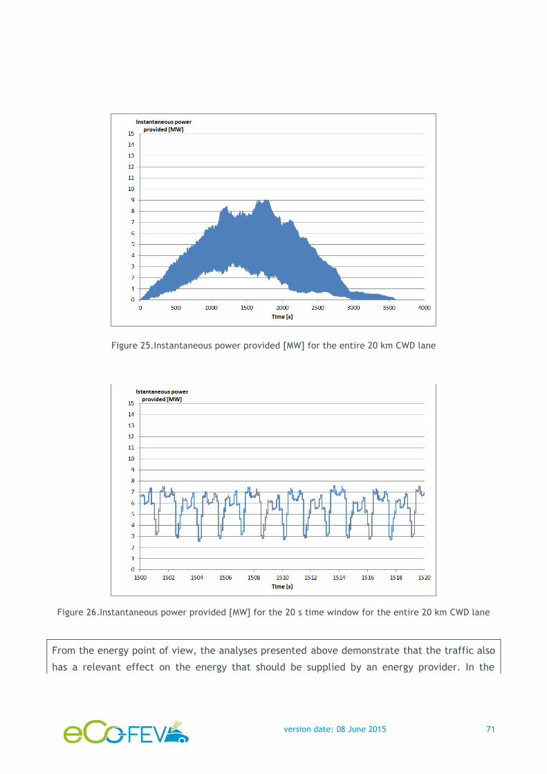
CWD system. The total time spent in the “en route” charging process can be estimated by

observing in the microsimulation all stopping events for all electric vehicles on the CZs. The

time is easily converted into energy by assuming an electric power for the CWD system.


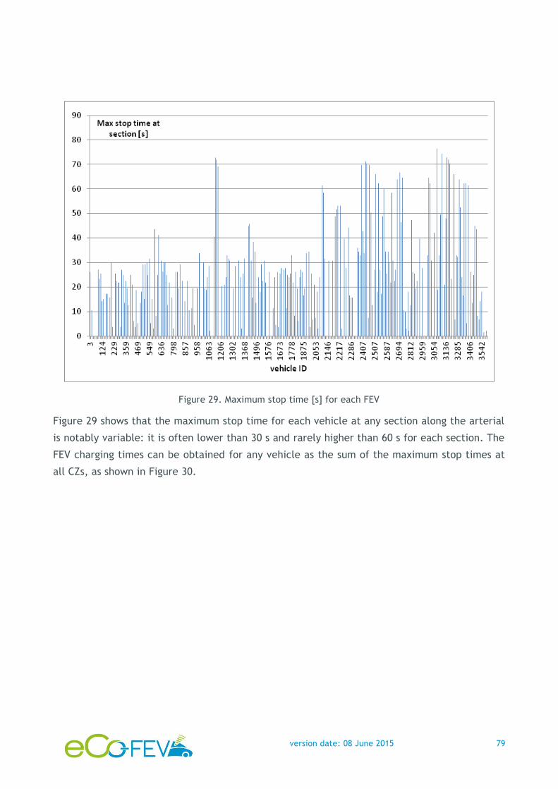
Figure 29. Maximum stop time [s] for each FEV

Figure 29 shows that the maximum stop time for each vehicle at any section along the arterial

is notably variable: it is often lower than 30 s and rarely higher than 60 s for each section. The

FEV charging times can be obtained for any vehicle as the sum of the maximum stop times at

all CZs, as shown in Figure 30.


Figure 30. Global charging time [s] for each FEV

Focusing on the energy gain provided by the CWD system, the energy consumed along various

routes in the road network should be compared to the energy received from various CZs.

The stop time values at CWD sections are converted into electric energy by assuming two

different powers (Pcz = 22 kW and Pcz = 50 kW).

To show the differences in energy balance for the two cases of provided electric power, in

Figure 31, a frequency analysis for both powers is reported for only the vehicles that crossed

the entire arterial. For the power of 22 kW, 50% of the vehicles had a negative balance, i.e.,

less than 100 Wh, which was calculated as the difference between the energy received from

the CWD system and the energy consumed. For this power, approximately 23% of the vehicles

had a positive energy balance, i.e., greater than 100 Wh along the arterial. As expected, for

the higher power of 50 kW, only 17% had a negative balance, whereas 58% might gain energy

after crossing the arterial.


Figure 31. Energy gains for FEV along the arterial

More details on this CWD scenario concerning an urban arterial application can be found in

Deflorio and Castello (2015).


3. Impact assessment concerning service quality adopting performance indicators

3.1. Key Performance Indicators

In the deliverable D400.2 a list of performance indicators was defined in order to be able to

evaluate the performance of the eCo-FEV system. Furthermore many lists of evaluation

datasets were defined that lead to the deduction of the performance indicators. During the

tests done in WP 420, and also with many lab tests, the validation and performance evaluation

were described in the deliverable D400.3. The following table shows a list of the deducted

performance indicators as result of the performance evaluation.

Performance Indicator

Description Target Value / Range

Observed Value or Behaviour

eCo-FEV Backend Message process latency

Average time difference of probe management database update time and VRMessage time stamp

10 s

2 seconds + network latency

eCo-FEV Backend Message process rate

Average time interval of probe management database update

60 10 s < 20 ms

Route search latency

Average time interval between route search request time stamp and KML time stamp

10 s The route calculation time depends on a number of factors: route length, number of charging stations needed up to the destination.

E.g. For a 200km route that uses 2 charging station out of a set of 50 charging stations: this metric is 6 seconds


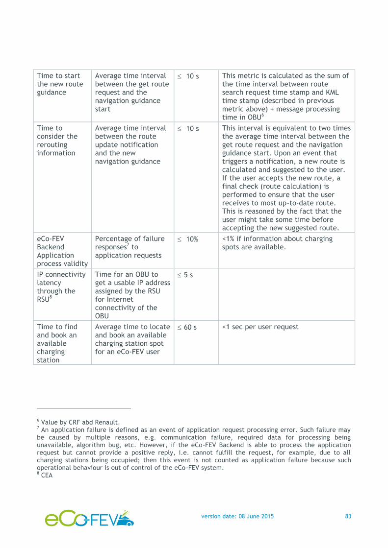
Time to start the new route guidance

Average time interval between the get route request and the navigation guidance start

10 s This metric is calculated as the sum of the time interval between route search request time stamp and KML time stamp (described in previous metric above) + message processing time in OBU6

Time to consider the rerouting information

Average time interval between the route update notification and the new navigation guidance

10 s This interval is equivalent to two times the average time interval between the get route request and the navigation guidance start. Upon an event that triggers a notification, a new route is calculated and suggested to the user. If the user accepts the new route, a final check (route calculation) is performed to ensure that the user receives to most up-to-date route. This is reasoned by the fact that the user might take some time before accepting the new suggested route.

eCo-FEV Backend Application process validity

Percentage of failure responses7 to application requests

10% <1% if information about charging spots are available.

IP connectivity latency through the RSU8

Time for an OBU to get a usable IP address assigned by the RSU for Internet connectivity of the OBU

5 s

Time to find and book an available charging station

Average time to locate and book an available charging station spot for an eCo-FEV user

60 s <1 sec per user request

6 Value by CRF abd Renault. 7 An application failure is defined as an event of application request processing error. Such failure may be caused by multiple reasons, e.g. communication failure, required data for processing being unavailable, algorithm bug, etc. However, if the eCo-FEV Backend is able to process the application request but cannot provide a positive reply, i.e. cannot fulfill the request, for example, due to all charging stations being occupied; then this event is not counted as application failure because such operational behaviour is out of control of the eCo-FEV system. 8 CEA


Time to authenticate for charging

Average time that elapses from the initiation of charging request to the reception of authentication (before the start of energy flow).

5 s The average time for inductive charging is 2,5 to 3,5 seconds including the ANPR detection

For the conductive charging over a narrow GPRS connection, the average time is 4 - 6 seconds (not crucial for the conductive charging use case).

Accuracy and timeliness of charging status accessibility information

Success (correctness) ratio of available/ busy status indicators for EVSEs provided by eCo-FEV to the user (ability to cope with accessibility changes)

95% 99.9%

The availability information is up-to-date and always pushed to the backend when a change occurs to any charging station.

Table 21. List of performance metrics for eCo-FEV service quality assessment

The results listed in Table 21 show that most targets of the performance indicators for the

eCo-FEV system are met.

The following sections focus on the charging infrastructure implemented in eCo-FEV. After a

short recall of its implementation architecture, the impact of the technology decision made in

the course of the project are discussed. Then it follows a description of the test-site where

conductive charging technology has been deployed. The last section describes in more detail

the evaluation of the inductive charging technology as a major development result of eCo-FEV.

After a description of the test-site where this technology was deployed, a detailed evaluation

of different electrical aspects of the inductive charging technology is conducted. This

evaluation considers the efficiency of the system, the security and EMF shielding, and the

behavior in case of misalignment. Thus this chapter covers the ICT aspects of the charging

infrastructure as well as the electrical power transmission aspects for the IPT.

3.2. Evaluation of charging infrastructure

The Service quality is affected by the very nature of the used and developed technologies on

one hand, and by the performance indicators gained from the validation and evaluation of

these technologies on the other hand. With focus on charging infrastructure system this


chapter discusses the impacts and side effects of the used technologies in the charging

infrastructure subsystem as described in the results of the WP300, while considering the

results of the evaluation from the WP430.

We recall that the Charging infrastructure System in eCo-FEV covers two power transfer

technologies - conductive power transfer and inductive power transfer - that contain inherent

differences not only regarding the power transfer itself, but also regarding the consequences

on the ICT systems operating the different technologies. At the same time the different

technologies need to exhibit analogical functionalities and services provided to the e-mobility

stake holders, such as user and / or Fully Electrical Vehicle (FEV) authentication and

authorisation, charging session accounting of the users or the FEV and then reporting the

Charging Data Records (CDR) to the respective energy provider, reservation services for users

and or electro mobility providers, and monitoring of the Electric Vehicle Supply Equipment

(EVSE), on one hand for the owner or operator of the EVSE, to make sure that the equipment is

working correctly and to be informed if it is not the case, and on the other hand to inform the

other electro mobility stake holders about the status of the EVSE such as availability

information and necessary technological parameters for the service provision.

These services are provided by the charging infrastructure system over different chains of

interfaces using different technologies. Thus the overall quality of the services is then

dependent on the performance of these interfaces and technologies used. Since the

architectural choices of the charging infrastructure system define and describe these

interfaces and technologies, a short recall of the architecture as described in D300.5 is

revised. Afterwards the impact of the technologies and the performance of the interfaces will

be discussed.

3.2.1. Interfaces and technologies of the architecture of the charging infrastructure system

This section provides a short revision of the architecture of the charging infrastructure system

as described in the deliverable D300.5, with an emphatisation on the interfaces and the

technological decisions involved in providing the afore mentioned services (also described in

deliverable D200.3) for the two different charging technologies deployed on the different test-

sites in eCo-FEV.


The charging infrastructure depicted in Figure 32 is composed of two different components the

Charging Station Control Unit (CSCU) and the Electric Vehicle Supply Equipment Operator

(EVSE-Operator). The CSCU is a hardware installed on site at the EVSE and the EVSE-Operator

is merely a service (more precisely a set of services) deployed in a server infrastructure. These

two components cooperate together to provide the different services such as Authentication,

Authorization and Accounting (AAA), Monitoring (both technical monitoring and availability

monitoring), and Booking (reservations of charging facility for EV users).

Figure 32. Charging infrastructure System

The EVSE-Operator communicates to the different CSCUs on the different Sites on one hand

and in his turn, provides a set of services for the eCo-FEV Back End over a Representational

State Transfer (REST) Web Service. Although the interface to the eCoFEV Back End is unified,

the communication to the CSCU depends on the different charging technology for which the

CSCU has been developed.

In general the CSCU needs to interface with the EV or its user for authentication and

authorisation triggering when the EV or EV’s user requests to charge. This is both the case for

inductive and conductive charging. Furthermore it is useful that the CSCU has a

communication link to the EVSE-Operator9 in order to check the AAA data of the EV user

requesting the charging service. The communication to the EVSE Operator is also needed to

provide information about the status of the EVSE especially for the operating staff of the EVSE-

9 Except the case were a white list of authorized EV or EV users is kept at the CSCU and no accounting information is also saved locally. This information has to be gathered manually by the operating staff of the EVSE-Operator.


Operator10 but also for providing the E-mobility providers with accessibility and availability

information. Last not least the interface between the EVSE-Operator and the EVSE is needed

for propagating reservations for certain EV users. The technologies used to provide these

different services over the CSCU-EVSE-Operator interface differ between the two test sites,

since they were developed for the two different technologies. Moreover the CSCU performs the

operations and services related to the control of the power transfer transparently to the user

however in coordination with the power electronics installed in the EVSE.

For the inductive charging technology on the Susa test-site, the CSCU has been developed in

eCo-FEV from scratch. Thus there were no specific limitations on the interface(s) between the

EVSE-Operator and CSCU, nor any limitations on the technologies used over these interfaces.

As described in D300.5 the CSCU at Susa test-site for inductive charging uses Remote

Authentication Dial In User Service (RADIUS) protocol for AAA, and Simple Network

Management Protocol (SNMP) for Monitoring and Booking. Aside of the CSCU – EVSE-Operator

interface, the CSCU, on Susa test-site, interfaces with the EV and the Power Electronics over a

serial CAN-Bus interface. This interface is not only used for the Charging Procedure Control

(CPC), but also used by the EV to trigger the charging request.

In contrary, for the conductive charging solution deployed in Grenoble test-site, a commercial

solution was installed. This means that the CSCU represents the microcontroller inside the

commercial EVSE, which transparently handles the CPC once an EV is charging. Nonetheless to

start a charging session the CSCU interfaces with the user that needs to hold the Radio

Frequency Identification (RFID) badge in from of the CSCU’s (or EVSE’s) reader. Furthermore

the commercial EVSE has a single interface that uses Open Charge Point Protocol (OCPP)

currently in the version 1.5, over which the EVSE-Operator can communicate to the EVSE’s

CSCU to provide all the services described before. E.g. for authenticating a users RFID trigger,

the ID of the RFID is then communicated by the CSCU to the EVSE-Operator, over the OCPP

interface. The OCPP interface further sends status information and Meter Values for the

ongoing charging sessions.

10 Otherwise the EVSE-Operator staff needs to check personally each EVSE in regular intervals to ensure correct operation.


Even though the CSCUs use different technologies the functionalities are analogic(al). The

EVSE-Operator has to implement the counter parts of these technologies to provide the

functionalities and services of the CSCUs. Furthermore the different technologies used by the

different CSCUs when communicating with the EVSE-Operator, are then aggregated at the

EVSE-Operator that implements a single REST-base interface, over which E-mobility providers

(such as eCo-FEV back End) can access the services of the charging infrastructure.

Figure 33. Technologies of the Charging Infrastructure

Figure 33 shows a summary of the different technologies implemented at the EVSE-Operator.

In the following section the impact of using different technologies will be analysed.

3.2.2. Technology impact assessment

As described, the technologies used and developed in WP300 are diverse, not only since

different charging technologies are considered but also from the point of view of the ICT

technologies used. This allows a comparison of these technologies for providing the different

services and under consideration of different aspects. Mainly the technologies used on the

CSCU-EVSE-Operator interface are different but also the CSCU’s EV user interface is

considered. On the CSCU-EVSE-Operator interface we have on one side OCPP, a Simple Object

Access Protocol (SOAP) based protocol for AAA, Monitoring and Booking, opposed by a

combination of SNMP and RADIUS protocols on the other hand.


3.2.2.1. Impact on the System modularity and the disintegration of the value chain under

consideration of the different roles in the e-mobility landscape

The services of the charging infrastructure map to different roles in the e-mobility landscape

regardless of the business model that will be in place once e-mobility is vastly deployed.

Following is a sketch of the some possible stakeholders in the e-mobility landscape:

EVSE manufacturer: knows the internals of the EVSE, is accountable for the correct

functioning and the secure operation of the power transfer.

EVSE maintainer: has maintenance staff that needs to be informed in case of faults.

EVSE owner: probably the landlord who invested in the EVSE, and probably expects

some revenue, or at least needs to know the usage and status of his EVSE.

Energy provider: needs to know to whom it provided how much energy

E-Mobility provider: who provided charging services to EV-users on “foreign EVSE”

Without claiming that this list is final and definitive, since the final business cases of e-

mobility are not completely set yet, but it is obvious that the data of the EVSE and the EVSE

users will be needed but rather many (theoretically independent) stakeholders then by only

one. Furthermore in case many stakeholders can access the EVSE for controlling and

monitoring, it is important to avoid conflicts and to keep sensible information from misuse.

Here comes the importance of the technological choices for meeting this requirement.

While OCPP protocol (per definition) does not foresee more than one endpoint, the EVSE will

communicate with only one stakeholder which avoids conflicts in policies and mitigates the

Information security risks given adequate IP security measures (IP security is considered in

later section). Furthermore using OCPP on the EVSE means the party implementing the OCPP

Central System (i.e. EVSE-Operator) has an advantage over other e-mobility stakeholders in

regard to the use of the specific EVSE. On the other hand in case the OCPP central system

fails, all connected EVSEs are affected. And all connected stakeholder loose the services at

these EVSEs.

The other solution implemented on the CSCU for inductive charging uses Simple Network

Management Protocol (SNMP) and Remote Authentication Dial In User Service (RADIUS). This

combination inherently foresees a fundamental separation between the use cases of the EVSE.

Status data acquisition, technical monitoring, and user authentication, authorisation, and

accounting could be done simultaneously by different parties. This is possible due to the


inherent properties of SNMP and RADIUS. SNMP, organises information in Management

Information Bases (MIBs). Each MIB has a tree structure for holding the information. For each

subtree, different access rights could be assigned to differentstakeholders. This allows the

simultaneous, conflict free access to the information on the EVSE. RADIUS configuration on the

EVSE not only allows the separation services but also allows setting a failover Authentication

server which increases the service availability.

3.2.2.2. Technology Impact on the IP networking and IP security related setup

The functionalities described above require a bidirectional communication between the EVSE’s

CSCU and the service’s counterpart. Yet there are differences between the two solutions in

this regard. Commonly the EVSE might be installed at some location where wired broadband

access is not necessarily available (e.g. the eCo-FEV test sites). For this reason, many EVSE

foresee the use of mobile broadband. Now while this technology reaches higher and higher

bandwidths the IP addresses (IPv4) are not fixed, either the mobile broadband ISP uses

carrier grade Network Address Translation (NAT) because of the restricted number of IPv4

addresses, putting the EVSE behind a firewall, or the ISP does provide a public IPv4 address,

but, it might dynamically changes.

Using IPv6 could be a solution although many mobile broadband ISP are reluctant in providing a

public IPv6 address to a SIM card, which inherently exposes the User Equipment (UE) to the

Internet, risking, not only attacks, but simply a so-called ping of death, i.e. pinging the known

IPv6 address of the UE until the battery is drained.

Assuming the use of public IPv4 addresses, the OCPP foresees that the EVSE includes its

current IP address in the SOAP messages, so that the central system knows how to reach the

EVSE for the bidirectional communication. How this is done depends on the implementation of

the OCPP protocol on each different EVSE. Another solution would be to use a Dynamic Domain

Name Service (DynDNS) service, this way the bidirectional communication will be using the

DNS name of each EVSE.

Both solutions assume the presence of a public IP address. The contracts with public IPv4

addresses tend to be more expensive then the one where NAT is used. In fact the connectivity

on the eCoFEV test sites does not use any public IP address, instead the EVSE is builds a Virtual

Private Network (VPN) connection over its uplink. This eliminates the problem of bidirectional

communication for both solutions.


Another important question when choosing the technology for future E-mobility infrastructure

is the bandwidth costs. Although the costs are gradually dropping for the costs of mobile

bandwidth, as the number of EVSEs grows, the bandwidth consumption might get relevant on

the EVSE’S counterpart. In case of OCPP, the central system will be the single counterpart. In

the version 1.5 and also in the version 2.0 OCPP uses a separate TCP connection for each

message. This includes a TCP connection setup and disconnection for each message by each

EVSE. On the other hand, SNMP and RADIUS use UDP, where no connection setup and turn

down are needed. This reduces the bandwidth needs by roughly by one eighth. OCPP could

increase the bandwidth efficiency by keeping one TCP connection open for sending multiple

messages instead of a connection setup and tear down for each one. The bandwidth effects

are very relevant when the uplink is very narrow like with GPRS.

The chosen technology impacts the possibilities of IP security measures. While OCPP foresees

the use of Transport Layer Security (TLS) by enabling secure Hyper Text Transfer Protocol

(HTTPS), for transporting the authentication Data, RADIUS supports flexible Authentication

methods using RADIUS Extensible Authenticating Protocol (EAP) supporting about 40 EAP

methods. Furthermore RADIUS inherently foresees forwarding AAA packets to another RADIUS

Server. In case the EV user’s data are not available at the serving RADIUS server the request is

forwarded to the EV user home server. This allows a discrimination free access to charging

services, with no additional implementation.

3.2.2.3. Technology Impact on the monitoring performance and validity

As regards the monitoring information, SNMP and OCPP differ in the information flow

direction: while SNMP allows querying the EVSE about its state, OCPP sends a (usually once)

message upon a state change. In case the message is not received by the Central System (e.g.

in case it is temporarily down) some implementations of OCPP on the EVSE cache the OCPP

messages in a backlog until the Central System is reachable again. If the EVSE do not cache the

messages and the Central System software crashes for any reason, the monitoring information

might not be valid anymore. Even if the EVSE caches OCPP Messages that has not been

received by the central system, the central system has persistently keep track of the

chronological state changes of each EVSE for instance in a local database.


Another issue with the validity of the monitoring information is the information about the

availability, especially for the conductive charging. When an EVSE reports that it is available,

this does not necessarily means that an EV user can charge at this same EVSE, if the parking

spot in front of the EVSE is used by another vehicle.

On the Grenoble Test Site parking sensor has been placed at the parking spots usually reserved

for charging EVs. For the inductive charging, the coil on the ground can detect if an EV is

above it or not, thus this problem is then automatically solved.

3.2.2.4. Technology impact on the implementation costs

In regards to the costs of the two different technologies, RADIUS and SNMP are Internet

Standards, described by RFCs of the IETF. Furthermore they are widely implemented and used.

Also there is a variety of free open source, as well as commercial implementations available

for those two protocols. The OCPP protocol specification – in contrast to what the name

suggests – is owned by a private company (e-laad.nl). It is available at the Open Charge

Alliance, and used to be openly accessible. Currently it is accessible upon registration, and

there is no real guarantee that it will stay under a cost-free license. Otherwise it uses SOAP

technology which is very much in trend especially in enterprise environments.


3.3. Test site realisation in Grenoble

Since March until September 2014, CG38 (since April 2015, renamed as “Le Département de

l'Isère”) defined the charging station specifications of eCo-FEV system and equipped the test

site with the adequate facilities.

A major issue was to specify the charging stations with the required characteristics, as

specified hereafter.

- To supply charging services for all users of this specific park ride, and particularly

o To supply all charging mode 1, charging mode 2 and charging mode 3.

o To supply both standard and accelerated charging modes

- To be operated on public domain

- To easily communicate with advanced services platform as eCo-FEV platform thanks to

adequate communication interfaces and to be easily integrated into V2X system

- To comply with sustainable scalable requirements, from an energy management point

of view.

The charging stations were installed in September 2014.

The charging station was equipped with E/F and T3/T2S socket and could support all charging

modes: mode 1, mode 2, mode 3 and could therefore supply electricity to a large range of

vehicles: different models of electrical cars but also vehicles like bike, tricycle, four-wheels-

cycle.

The charging stations can supply different levels of power: 3, 7, 11, 22 kW, according to the

owner; it we expect implictly that in general it should be capable to deliver all the power

levels in the range below 22 kW, not only those indicated

Consequently different use cases could be experimented.

- The standard (slow) charging mode at 3kW is adapted for EV users who park their

electrical vehicle during a day or half a day and who use express bus lines, car sharing

or cycle track to reach Grenoble area (for work, business, shopping, hobby purposes)

- The accelerated charging mode at 7, 11, 22 kW is adapted for EV users who park their

electrical vehicle for one or a few hours (for example for hobby on interurban

bikeways). Partial quicker EV charging (around a few tens of minutes on 22 KW) can be

used if needed.

- It is important to outline that this possibility of several charging modes lead to

substantially enrich the eCo-FEV advanced services experimentation: different

scenarios are possible for the use cases experimentation; according to the choice of


charging mode, different battery autonomy strategies and routing strategies are

proposed and more diversified EV user needs can be targeted.

To operate on the public domain, charging stations are equipped with RFID card access system,

anti-vandalism mechanism and can be controlled by a supervisory system. Signs enable to keep

two park slots for EV charging in a car park ride which is much used on a daily basis.

Issues are essential: the car park ride is relatively isolated in a suburban area: more precisely

it is located just at the entry of the Grenoble urban area; from this point, and in case of

traffic congestion, car park users may catch express buses allowed to use dedicated lines or

they may use cycle track. Therefore, this type of location required to be managed. Access

management and anti-vandalism are particularly required.

The French test site include:

- Charging stations equipped with a communication interface

- A road side unit which ensures the connectivity of the vehicle, by using 802.11.p

protocol.

- An internet router which ensures the internet connectivity of the site (4G cellular

network)

- An Ethernet LAN (Local Area Network) to connect together charging stations, router and

road side unit.

The communication interface :

- Communication with eCo-FEV backend is supported by OCPP 1.5 protocol thanks to

adequate interface. Ethernet interface enables to connect charging stations to the LAN

(The including a router which ensures internet communication with eCo-FEV back-end

platform. A LAN is required to also ensure the internet connectivity of vehicle through

Road Side Unit.)

- Communication with a specific energy management system is supported by specific

Modbus protocol

- A possible evolution with ISO-15118 standard is specified, such an evolution should be

implemented according to ISO-15118 achievement status and eCo-FEV achievement

status.

Status of the work progress done between March and August 2014:

- The different specifications for charging stations were elaborated: technical

specifications were achieved.

- Communication interfaces were discussed and specified. A consensus between the

partners was elaborated.


- A pre commercial mode of charging station was identified. These charging stations have

the following characteristics:

o Compliance with the technical specifications

o Innovative design for operation on public domain

o Required communication interfaces

o Upgradeable for participation to Eco-FEV experimentation

- A contract was signed for supply and installation of these charging stations. The

contract includes technical and administrative specifications. It enables to procure pre-

commercial charging station, which are both industrially mature and innovative

upgradeable enough for complying with the eCo-FEV experimentation requirement.

- The connection to electrical distribution grid was done. A 36 kVA energy access point

was chosen. Energy management system enables to propose up to 22KW charging mode

as limiting the power demand if necessary. This power level enables to limit the

connection costs (“blue grid connection traffic in France”). Moreover from a high

scalability point of view, such a strategy enables to limit the economic costs of grid

investment and to limit the contribution to local and national electrical load peak.

- The laboratory communication tests between eCo-FEV platform and charging station

from charging station supplier laboratory were done to test OCPP1.5 communication

protocol.

- The architecture and component of local area network were defined, a consensus was

built. There are still discussions about IPv4 and IPv6

During September 2014:

- The location of charging stations was definitively defined.

- The Civil engineering works (including concrete platform building, electrical and

communication cable arrangement) were achieved to make the charging station

installation possible

- Horizontal and vertical marking are achieved

- The installation and test of charging station are in progress.

Test of charging stations on the French test site were carried out successfully in 2014

(19.11.14).

The two charging stations have been tested for the correct operation.

- A charging station works for normal or lightly accelerated EV charge 3 or 7 kW


(supplying two charging points);

- A charging station works for accelerated EV charge 11 or 22 kW (supplying two charging

points)

The test carried out have enabled to validate:

- Materials and civil working;

- Energy supply, RFID card access and optionnal Schneider supervision (for data

collection and EVSE management in public domain

Simultaneous charging of four vehicles - including 2 ZOEs, 1 Kangoo and 1 Fluenze - were

successfuly implemented.The OCPP1.5 tests have been successfully implemented in 2015.

Similar tests as those carried out in August 2014 were successfully completed in Schneider

labs, by using a CG38 IPv4 router, as required by the company itself . The same company

implemented the procedure to configure the charging, illstarting this to the manager of the

systems.

- In 2015:

o Schneider implemented the procedure to configure charging station (OPCC1.5 or

classical supervision) for confirm subsequent tests;

o CG38 / the Département de l'Isère and CEA supplied the needed SIM card for

internet access on French test site (VPN or static IP address, as decided

subsequently).

o TUB finalised the software details (“change and get configuration”)

o CG38/ the Département de l'Isère operated on the electrical vehicle

- Aa final test with OCPP1.5 configuration has been foreseen and carried out, with at

least one real Electrical Vehicle, with at least a router (CG38), though possibly with

aCEA router as support: the procurement of charging station would be achieved.

- After the availability of the charging station for eCo-FEV and related advanced tests,

experimentations were thereafter possible for the final demo in Genoble (May 2015).


3.4. Installation and evaluation of inductive charging

3.4.1. Test site: installation and first trials at the test site in Italy

Since March until June 2014, TECNOSITAF, with POLITO and CRF support, completed the

planned works (Figure 34) concerning the implementation of a test site in accordance with the

eCo-FEV project requirements. It is worthy to underline the works have been completed in

accordance with the eCo-FEV Gannt: in fact, at the end of June 2014, TECNOSITAF staff

finished its job, in order to permit the start of the activities (installation and integration) of

the other Partners. The lists of work follows hereafter.

Figure 34. Test site area

3.4.1.1. External works

- Renovation and cleaning of the area dedicated for the test site

- Definition of the requirements of the test site:

o Performances in term of electric charging

o Integration with the existing Safety Track

- Planning of the civil works

- Concrete paving to create a Parking for the Static Recharge


Figure 35. Static wireless recharging zone

- Several excavations were made to place the cables dedicated to the interconnection

between Control Room, Power Room, Charge Zone and all Components of the test site

- Installation of several manholes along the excavations route were made to facilitate the

cable inspection

Figure 36. Excavations

- Laying of Power cables and FTP cables

- Small concrete paving for the shelter installation

- Installation of the Shelters, one for the Static Recharge and one for Dynamic Recharge


Figure 37. Shelter

- Cuts of the pavement (asphalt) to connect the shelters to the Recharge Coils; one cut on

the Park (Static Recharge) and one on the road (Dynamic Recharge)

- Installation of a manhole in the centre of the Park for coils connection (Static Recharge)

- Installation of a manhole at the end of the asphalt cut for coils connection (Dynamic

Recharge)

Figure 38. Area for the wireless recharging in motion

- Connection the test site to the Network by ICA-NET solution11; installation of: Antenna,

switch, WiFi router and cable

- Installation of the ANPR Camera

11 http://www.ica-net.it/chisiamo.asp

http://www.ica-net.it/chisiamo.asp


Figure 39. ANPR

3.4.1.2. Internal works

- Renovation of the existing building in order to accommodate the Control and Power

Room

Figure 40. Exhisting builing

3.4.2. Power Room

- Renovation of the existing Power Room

- Renovation and cleaning of the existing Power Transformer

- Study and planning the electric works

- Installation of the new Power Transformer dedicated to the coils power supply


- Installation of the ducts to connect all cables

- Laying the cables to connect the Power Room with the Control Room and the Recharge

Zone

- Installation of the electric panels to manage the power supply

Figure 41. Power Transformer

Figure 42. Power Room

3.4.2.1. Control Room

- Renovation and cleaning of the existing Room to accommodate the ECo-FEV Control

Room


- Study and planning the electric and hydraulic works

- Tinting the walls

- Change the lighting system

- Installation of the ducts for cables connection

- Laying the cables to connect the Control Room with the Power Room, the ANPR

Camera, the Internet Antenna and the Recharge Zone

- Installation of the electric panels to manage the power supply

- Installation of the UPS system

- Connect the office lighting, office sockets and electronic management line to UPS

- Installation of the air condition/heating system

- Provide the Control Room furniture

- Predisposition of several work locations

- Hydraulic work to repair the existing toilet

- Installation of a boiler in order to provide the hot water

Figure 43. Control room

Figure 44. Work location


3.4.2.2. Vehicles Recovery

- Renovation and cleaning the existing Garage dedicated to recovery the ECo-FEV

vehicles

- Installation of a Power Plug-in to recharge the electric vehicles

- Installation of an electric panel to manage the Plug-in recharge

Figure 45. Plug in

3.4.2.3. ANPR SOLUTION

Automatic Number Plate Recognition – ANPR, also called Automatic License Plate Recognition –

ALPR, is an enforcement technology that optically scans vehicle license plates in order to

design an efficient automatic authorized vehicle identification system by using the vehicle

number plate.

The developed system first detects the vehicle and then captures the vehicle image. Vehicle

number plate region is extracted using the image segmentation in an image. Optical Character

Recognition – OCR technique is used for the character recognition. The resulting data is then

used to compare with the records on a database so as to come up with the specific information

like the vehicle owner, place of registration, address, etc.

This rapidly deployable, scalable solution uses rugged infrared cameras that connect to

leading-edge optical character recognition technology software, allowing to conduct

surveillance under varied lighting and weather conditions.

ANPR / ALPR process is useful in many scenarios, for example:

- Automatically opening gates / doors for authorized vehicles

- Traffic monitoring and recognition

- Toll collection systems

- Car Park usage monitoring


The Automatic Number Plate Recognition – ANPR includes the following processes:

- Image Handler. It is responsible for getting raw live images from the IR or color

cameras and transforming them into GIF, TIF or JPEG formats used by the OCR

process. The Image Handler also sends non-transformed images to ANPR

manager process.

- OCR. This process finds the plate numbers of the observed vehicle. These

results are sent to ANPR Manager process for further handling.

- ANPR Manager Process. This module transforms the live images to the images

formats used by the Web Server Process and sends them to it. It is responsible

for checking whether the found number plate matches the ones given into the

black and white verification lists of Data Base.

3.4.2.4. ICA-NET SOLUTION

ICA-NET is an Internet Provider that work in the Susa Valley Area.

Their solution is based on the Point to Multipoint Communication and it is the only provider

that guarantee the Internet requirements in the test site area in accordance with the project.

ICA-Net provide us the following equipment:

- Antenna

- Power supply and FTP cables for the Antenna

- WiFi router

3.4.2.5. Futrther steps

A list of the TECNOSITAF subsequent steps to complete the test site work in accordance with

the project follows hereafter:

- Support POLITO and CRF in their HW installation (in accordance with Polito and

CRF work plan).

- Cabling of the CRF and Polito equipment (in accordance with Polito and CRF

work plan).

- Installation of a surveillance system to guarantee the control inside the test

site area


- The safety procedures to guarantee the safety work for the tester have been

defined. The editing of the document collecting the procedures is work in

progress

- Hang up some ECo-FEV banners inside the test site area

3.4.3. Scope of the evaluation

The test on the inductive power transfer system in CWD have had several purposes, summarised

in the following list:

Evaluation of the overall efficiency of the IPT CWD system;

Evaluation of the behaviour in misalignment conditions;

Test of the effectiveness of the adopted power electronic structure and individuation of

criticisms;

Tests on the shielding system for human being EMF protection.

All this part is resumed in this document as far as useful for the overall evaluation while the

D.400.3 is the main destination of its more detailed analysis and reporting.

3.4.4. Description

The structure depicted in Figure 46 has been built in order to test the CWD prototype in indoor

condition.

The structure is composed by a fixed part - which emulates the ground pavement and over which

three transmitting coils are placed - and a movable structure, emulating the vehicle.

The movable structure sustains the receiving structure with the aluminium shield, allowing the

reproduction of different conditions of positioning, in three directions.

The system has been supplied through the same power electronics structures adopted for the

eCo-FEV test site, in Susa (Torino) .

The measurement of the magnetic field inductance has been conducted using an isotropic

exposure level tester ELT-400 shown in the Figure 46.


Figure 46. Prototypal structure for the laboratory test of the IPT CWD system (Politecnico di Torino, energy area Laboratory, April 2015)

3.4.5. Results

3.4.5.1. Evaluation of the overall efficiency of the IPT CWD system

The overall efficiency of the system has been evaluated on the passage over three transmitting

coils measuring the efficiency from DC side (AC/DC converter output) to DC side (HF/DC

converter output) as depicted in Figure 47.


Figure 47. Efficiency calculation scheme

The power transfer start is characterised by the shape of the current shown in Figure 48 where

it is visible a transient overshoot of the typical of the turn on phase of each transmitting coil.

The turn off phase that is commanded when the vehicle is passing over the transmitting coil, is

faster than the turn off phase as visible in Figure 49.

Figure 48. Turn ON of a transmitting coil with the presence of the vehicle


Figure 49. Turn OFF of a transmitting coil

The efficiency is evaluated as the mean efficiency measured over the complete charge

procedure and is resulted so far (end of April 2015) equal to

η = 84.3 %

This value is not effected by the speed of the vehicle because the power transfer is related only

to the electromagnetic parameters of the transmitting and receiving structures; the speed of the

vehicle is negligible respect to the typical time/frequency of the electromagnetic phenomena.

This means that the power transfer and the transient phases of turn on and turn off remain

independent by the vehicle speed.

Nevertheless, the speed of the vehicle represents a limit in relation with two aspects:

The power needed by the vehicle increases in a cubic way with the speed so there is a

speed limit after that the absorbed power from the battery starts to exceed the power

transferred through the IPT CWD system. This means that, the energy balance at the end

of the charge process becomes negative.


This speed depends by the vehicle weight and by the efficiency of the vehicle power train

and, in the case of the electric Daily adopted in the eCo-FEV project this limit is of about

50 km/h for the test site coil positioning.

The control of the DC/HF converter that supplies the transmitting coils becomes difficult

if the speed of the vehicle is too high. This difficulty is related to the actual architecture

of the power electronics that shares an “inverter leg” for two consecutive coils. The

passage of the vehicle from one coil to the next one asks for the change of the supplied

coil. This means to change the involved legs of the converter maintaining one leg shared.

While this solution is suitable for low speed and it represents a strong reduction of the

costs, it was revealed not so robust if the speed of the vehicle exceed 30 km/h. After this

limit point the fast turn-off/turn on operations causes big oscillations in the power

absorbed by the electrical network and it is not so tolerable by the power electronic on

vehicle board.

This is one of the most important results of the experimental tests because it provided

important information that will be the basis for future improvement in the design of

new power electronic structures with a more robust control.

3.4.5.2. Evaluation of the behaviour in misalignment conditions

The misalignment changes the power transfer capability and the efficiency of the system. This

dependency was tested and the main results are depicted in Figure 50 and Figure 51. The tests

were provided in static condition with the receiver centred respect to the middle transmitting

coil.


Figure 50. Horizontal misalignment test

Figure 51. Vertical misalignment test

These tests demonstrated the dependency of the power transfer capability and efficiency by the

misalignment respect to the nominal position conditions.


The misalignment causes a variation of the magnetic coupling between the receiving and

transmitting coils that is the main physical quantity involved in the inductive power transfer.

This aspect is object of present studies, that are trying to manage and control this variation

adopting an active converter system also on vehicle board instead of the simple diode bridge

proposed in the eCo-FEV prototype.

3.4.5.3. Test of the effectiveness of the adopted power electronic structure and

individuation of criticisms

The power electronics that supplies the transmitting coils and the converter on vehicle board

were tested to demonstrate their functionality and point out some aspects that need

improvement.

In addition to the previous underlined aspects, there are some other good results and opened

problem derived from the test that are here briefly summarised.

The eCo-FEV system implemented a procedure for the identification of the presence of

the vehicle only through the power electronic on ground. The proposed technique is well

functioning but it is the principal cause of the difference in the efficiency with respect to

the static charge and with respect to the dynamic one.

Static charge takes place in condition of good alignment with the presence of the vehicle

that can be confirmed with more accurate methods, according to the slow speed of the

operation.

In this case, the tested overall efficiency is about 87.3% (as visible in Figure 50 and

Figure 51 at the nominal distance of the two coils of 20 cm).

In the dynamic charge, all these aspects are deputised to the power electronic. As shown

in Figure 52, in case of absence of the vehicle a huge current is provided by the power

electronic without power transfer. This means that all this current generates losses over

the electronic switches and the coil resistance.


Figure 52. Procedure for vehicle identification through the DC/HF converter

This technique can be improved and it will be related with the future design process.

It is confirmed that the proposed structure, with a constant voltage on the transmitting

side, is a powerful choice. Its characteristic of efficiency, good controllability and

cheapness has been confirmed.

More efforts have to be spent in the future in order to improve the control in the passage

of the vehicle to one coil to the closer one. In the present phase, the same technique of

individuation of the vehicle is implemented so the same problems related to the

efficiency of the process occur.

The proposed structure that supplies more coils can reveal thermal problems in the case

where more vehicles are supplied at the same time. These problem increases if the

vehicles stop over the coils. All these aspects are leading towards the adoption of a


different power electronic architecture with a single H-bridge is dedicated to each

transmitting coil.

3.4.5.4. Tests on the shielding system for human being EMF protection

A set of measurement has been performed to verify the respect of the limit on the human

exposure to the magnetic field provided by the ICNIRP guidelines for limiting exposure to time‐

varying electric and magnetic fields (1Hz – 100 kHz) in relation with the public.

These measurement pointed out a series of criticisms in the shielding related to the movement

of the vehicle of the supplied transmitting coil.

The figure below summarises the different possible conditions of positioning during the charge

operation that have been analysed.


The conditions indicated with a red cross are particular condition where a supplied transmitting

coil is not totally covered by the vehicle and the adoption of a shielding system is practically

impossible. Has to be underlined that one of these cases is a fault condition and the other one

where the transmitting coil is only partially covered, is a condition that need for other and more

precise evaluations and that could be lead to the adoption of other kind of shielding solution or

safety procedure.

It has to be underlined that the red crossed conditions are dictated by the position of the

receiver that, in the case of the prototypal version mounted under the adopted vehicle, is not

centred respect to the vehicle chassis.

With the receiver placed on the centre, each active transmitting coil is covered by the vehicle.

This condition allows having a natural shielding of the magnetic field and a more suitable

condition for the management of the protection of humans close to the vehicle.

Figure 53. Measurement of the magnetic field induction during the operation of the system, at the Energy Laboratory (Politecnico di Torino, Dept.DENERG)


4. Impact assessment on mobility: general viewpoint and users

The analysis of effects of FEV and services related to ECO-FEV is split into two parts: a general

viewpoint and possible users, included within this chapter, and the analysis of the possible

demand, in the subsequent one.

4.1. Mobility in a shared vision for FEV

FEV are entering the market through various paths: from electric car sharing to electric fleets

for urban services, besides the introduction of electric motors in various hybrid forms, which

seem to be nowadays and for a number of years the actual and pursuable path towards a more

oil-independent transport economy, thereafter more environmentally friendly.

FEV have anyway a number of possibilities in the new motorised mobility declination that are

analysed hereafter, taking into account the role of eCo-FEV specific services, both for wired,

conductive, charging and for the inductive one, through CWD. User needs are taken into

adequate account, though the analysis on the demand is taken into account in the subsequent

chapter.

4.1.1. New mobility paradigms: car sharing

In recent years new mobility paradigms have come fore: these systems are based on a new

idea of innovative motorised mobility. Probably the most popular one is the well-known car

sharing: it allows drivers to have a wide range of, sometimes different, vehicles available

nearly any time as needed and typically users pay only for what and how much the service is

used, without maintenance fixed costs, refuelling, taxes and insurance that are usually

connected with an own property car.

The car sharing system is an unconventional service that might represent, in cities, an

efficient alternative to the current idea of motorised mobility. If we consider the source12 by

which in Europe 80% of urban circulating vehicles travel no more than sixty minutes per day

12 http://www.icscarsharing.it/main/carsharing

http://www.icscarsharing.it/main/carsharing


transporting averagely 1,2 person, a car sharing user can drive a car for the time it is needed,

and more people can use the same vehicle.

The service is typically available 24 hours a day, can reduce the environmental impact of

vehicle circulation, and may decrease costs but increases parking space and the opportunities

for the users to choose the right vehicle for their specific needs.

In this way, it can occur that there will be a lower number of cars circulating on our streets

and the number of parking spots available may increase, quite a concerned issue for most of

cities.

The competitive advantage of this service lies on the originality of the supply: the

performances are similar to the private car ones, but typically at lower price. The automotive

market does offer a high variety for buying a car, but not very much for those who use it

occasionally. So car sharing can by also seen a modern, smart and eco-friendly four-wheel

approach, a useful and favourable choice, which contributes to reduce problems of traffic and

pollution.

It was firstly introduced in Switzerland nearly thirty years ago and later it developed in

Germany, Austria, Netherlands, Scandinavia and United Kingdom. Today it is a well-

consolidated service in United States and Northern Europe.

The present young people generation cannot afford to own a car, for this reason Car Sharing is

sometimes successful.

In Berlin, car sharing has revolutionised: it is not by chance that the most experimenting town

has also the youngest population in Europe. Thanks to its under thirties population, often

unemployed and without a car, this city is on the top score in car sharing in Europe.

Christoph Menzel, mobility researcher, said “car sharing existed for thirty years, the

innovation is the smartphone technology that will transform in the next 3 to 5 years urban

transport, integrating cars, bicycles, and public transport”. Earlier in time, cars were rented

and carried back in the same spot, now you can search for it on a App or on the web and find

it.

Large investments were made from the automotive sector involving large companies such as

Mercedes with the service called “Car2Go” (1200 Smart), BMW with “Drive Now” (800 cars,

mostly Mini), Citroen with the Multicity electric cars (300), and German railways (mixed fleet).


The electrification of European vehicles, mainly in urban contexts, can be easily matched with

this new style of motorised mobility, shared, provided that mobility preferences and constrains

are respected (chapter 5). In this way, the charge issue may be solved thanks to the park-

while-charging systems and the billing procedure that can be calculated as a whole service.

The French examples of Paris and Lyon show that this is already put in place.

In Paris, the service is called “Autolib” and it counts 2000 vehicles 100% electric located in

4000 stations, while Lyon has 34 different stations that hold 100 vehicles divided in three

different categories.

In Italy, the present car Sharing is available in Bologna, Brescia, Firenze, Genoa, Milan,

Palermo, Parma, Padua, Rome, Savona, Turin and Venice, with a total of 594 cars, 400 parking

spots and 21874 users13 [data updated in April 2014]

In the city of Milan three different suppliers are present: ATM, Car2go and finally the new

service by Eni called Enjoy. Since its beginning in 2002 Atm has been available with 135

vehicles called GuidaMi and 5.400 users. Car2go has 410 vehicles and a target of 30.000 users

by August 2014, while the Enjoy solution offers 600 models of Fiat 500.

The city of Turin since 2015 has two main services. In Turin the first car sharing was available

since the late 90s with the Electra park made with Fiat Panda. The present service in Turin is

called CarCityClub and has been active in town since December 2002. At the beginning of 2015

it was possible to use 41 cars available for 646 members and 24 parking areas. Since July 2014

electric Fiat 500 have been let available in different points of the city. In 2014 the Piemonte

Region has made a two-steps tender for free flow car sharing, with deadline in January 2015

for the second phase. Innovative ITS solutions have been appreciated for the bid.

While in Naples this service has been launched in 2014 with the name of Ci.Ro (City Roaming),

a car sharing and van sharing project whose vehicles are 100% electric.

A survey made by CarCityClub calculated the benefit for the environment thanks to the people

who selected this system: a decrease of 1250 cars circulating, a reduction of approximately 5

million km travelled and a decrease of 268 ton CO2 emitted.

13 http://www.icscarsharing.it/main/


A service of shared cars is convenient for those people who use it sporadically. Families who

own one or more cars, and in few cases need to use another one, can combine a property one

with a shared one when necessary. Moreover it is an interesting solution for those who want to

choose a different type of vehicle every time, from smaller to bigger ones.

These solutions are very appropriate for the technology of xEVs: the problem of reduced

independence is solved in the sense that car sharing is mainly an urban service. Secondly,

recharging can be made in the parking stations and the number of necessary charging points is

reduced because more vehicles can be charged on the same charging station.

In this way the same vehicle can be driven by many users, so the number of cars can be

drastically reduced, with a consistent increase of benefits.

The users of car sharing in Europe and USA are approximately one million, but in the next few

years the fleet will increase significantly reaching 70.000 vehicles in 2017 and 130.000 by 2020

in Europe. The number of users in Europe shall reach 8 million by 202014.

What drives people toward a shared car is, in primis, the economic factor: 56% of users

indicate as the most important reason not to buy a car its high purchase and maintenance

costs; only 23% takes into account pollution reduction.

Another car sharing strong point is how easy is to access the service, as shown by 36% of users.

There are critical areas to improve, such as the non-availability of a vehicle, of the desired

model and the doubt that in long term there will be a real saving.

The key factor is however, the cost, still high for many customers, but 64% of users believe

they will increasingly use this service.

In the next 6 years the sales of cars in USA and Europe, according to mentioned source15, may

decrease by 4,1 millions: 51% of users declare that thanks to car sharing avoided to buy a new

car and 45% foresee not to do it in the next future.

14 http://www.ecodallecitta.it/notizie.php?id=378794 15 http://www.ecodallecitta.it/notizie.php?id=378794


We need anyway to consider that, if more oil independent cars shall be the future of road

private transport, these shall be evidently more expensive than the more traditional cars,

based on ICEs; when a person or a family cannot afford these new vehicles, conserving an ICE-

based car for medium and long travels (more than 150 km indicatively, can be compliant with

daily motorised mobility in urban areas, especially when and where restriction to ICE are

applied, if a rentable FEV car is available in sharing, so constituting a migration plan towards

the period when an hybrid or a FEV shall be affordable by this person or family.

The trend to avoid buying a new car is stronger in metropolitan areas with high population.

These are the perfect or most suitable conditions for the spreading of this service, also

because it allows economies of scale.

4.1.2. Car pooling

Other emerging patterns of shared mobility are car-pooling and ride sharing services. The first

one is a sustainable way of transport thought for short distances and displacements made

mostly by commuters who share the car typically for home - work routes. They usually are

fixed crews that everyday drive along the same route.

Also in this new or recent approach, there can exist lots of advantages in terms of congestion,

environment pollution, and noise pollution, but it cannot be easily developed with electric

vehicles as car sharing.

Carpooling.it is one of the most popular and oldest platforms of sharing the same vehicle. One

of the related studies shows that, assuming an average emission of 155 gCO2/km and 220

working days per year, for a 10 km way if ten participants share the car, there would be an

yearly saving of 7 ton CO2, 14 ton CO2 if the passengers are 20.

More difficult is this connection: FEV - ride sharing, that is long distance trips shared in order

to split costs, due to the limited range of the current electric vehicles.


4.1.3. Possible conflicts

Even if the society seems to respond enthusiastically to these new business concepts, some

organisations and governmental institutions have started complaining. They argue about the

still undefined grey regulation area in which the sharing economy is moving, because of its

immaterial form and online accessibility.

Some already popular and efficient – though not completely legal - businesses like Airbnb or

Uber, which provide respectively accommodations and transportations based on renting or

sharing services, have started being limited in different cities and countries. A new law passed

in the city of New York, in 2010, which does not allow people to rent out rooms or their whole

apartments for less than a month, unless they are not living in the property at the same time

(The Economist Newspaper Limited, 2013a). Some cities like Brussels, but also many others,

decided to forbid their citizens to use the Uber service for car sharing; in Seattle, the number

of active drivers providing car sharing has been limited to 150 per time (The Economist

Newspaper Limited, 2014).

The main questions arise from the difficulties in making tenants and owners pay taxes and

follow the local laws, as well as provide legal insurance and defend people’s rights. It is

important for local authorities, and in general the economy, to keep track of the profits

people are able to get out of these activities, and to guarantee safety and rights.

Some of these peer-businesses have also been forced to engage themselves in insurance

services and more severe terms of contract, because of problems due to the lack or the

inefficiency of self-regulation systems currently in use, which rely on social networks and

customers’ ratings and reviews.

4.1.4. Sharing economy trend

Following the present sharing economy trend, as suggested by Brian Chesky in the Friedman’s

New York Times article Welcome to the ‘Sharing Economy’ (2013), these projects have the

potential of supporting and being part of innovative lifestyles based on the peer-to-peer rental

consumption, which is going to have a great impact on the market, as it has already been

estimated to worth $26 billion at global level (The Economist Newspaper Limited, 2013b). In

the UK it has been proved how it already affected the retail business, accounting for £22.4

billion on the British market (De Lecaros Aquise, 2014).


In the long-term perspective, it is estimated that people will change their habits and their

consumption behaviour. The service has the potential to stimulate a different approach to

many commodities. This will turn out to provide considerable environmental and economic

benefits for the nature and the society respectively, as it has already been the case for other

sharing services (The Economist Newspaper Limited, 2013).

Anyway, there are good chances to succeed. For example, in the UK it has been revealed that

the main reasons why people choose to use a peer-to-peer service instead than buying new

commodities, is the cost per use of the product.

For what concerns electro-mobility we usually have in mind considerations and assumptions in

the framework of replacing one traditional vehicle with an electric one. However, it is

appropriate and a further step in the analysis of future mobility to compare an electric vehicle

for private use with an electric vehicle used in car sharing.

12, 4 million electric vehicles expected in 2020 for private use correspond to the same number

of users, if we consider a one-to-one relationship between owner and car.

The comparison between EVs and Car Sharing is economically feasible. The users still have a

huge economic advantage as already mentioned, but such advantages are not automatically

transferred for an ecologic point of view.

If we consider the framework where a user drives a shared car instead of its own, but it does

not change his driving habits (35-40 km/day), then the emissions into the air will not change.

The available parking spots will increase but not the circulating vehicles.

However we must consider that the car sharing users significantly change their driving habits.

In a survey by ICS, they declare that:

1/3 has decreased the use of car

1/3 has experiences a decrease of travel costs

the decrease in kilometres is approximately 26,7% per year.

As per the frequency, also the number of kilometres travelled each year is lower. 12% drives

up to 2.500 km per year, 25% between 2.500 and 10.000, 26% between10.000 km and 17.000

km, 20% more than 17.000 km (ICS, 2009). These are Italian national data, but we can

estimate them as a valid European portion.


We can consider a yearly average of 8.773 km/year and therefore 24 km/day and a lower

number of kilometres but at higher rate if we consider that one single car is used by more

consumers.

It is thus very hard to establish quantitative relationship between EV diffusion and car sharing.

This mobility is for sure spreading and increasing in consensus, as well as we have seen that

there is a high potential for EVs.

Few non-quantitative observations concerning this relationship must be done.

Today, years 2014/15, we can say that car sharing system is a winning system, but in the case

where it is a private provider and not a public one.

We have also seen that electric vehicles have high potential in terms of profitability, so the

question is how to match the two of them?

Let’s try. If we imagine a world of car shared that are electric, then the service provider can:

decrease maintenance costs, because they are lower for electric vehicles than for

“traditional” ones;

decrease the fuel costs, as the electricity is cheaper than gasoline, given a certain run

distance

The consequence is a higher margin that can take advantage by increase the fleet and

decrease the costs for the user. In this case, he will be able to increase the percentage of car

sharing usage, and consequently the percentage of users.

The provider must also sustain the infrastructure costs, but in the case they are in few points,

as can be for big parking spots, he will be able to increase hugely the exploitation of the

charging points. Otherwise, if they are spread on the territory, as Eni and Car2go users that

can leave the car everywhere in the city, then he will have to set charging point everywhere.

However, he can try to saturate their use by offering to third parties a charging service.


4.2. Economic viewpoint for the user

We consider the microeconomic user’s point of view. By calculating the difference in price per

kilometre between a fuel combustion vehicle and an electric one, interesting results can be

found.

Imagine an hypothetical situation of a daily average distance of 40 km, the present European

price for fuel and electricity, let’s evaluate the amount of money spent for 12,04 million

vehicles in a year.

Fuel:

o Daily distance: 40 km/day

o 12 km/l 16

o price EU 27: 1,475 €/l 17

4,9 €/day

4,9 €/day * 365 day/y = 1788,5 €/y

Electricity:

o Daily distance: 40 km/day

o 0,12 kWh/km18

o price EU 27: 0,187 €/kWh 19

0,89 €/day

0,89 €/day * 365 day/y = 324,85 €/y

This means that each year the possible saving for a final user is:

1788,5 €/y - 324,85 €/y = 1463,65 €/y

16 source: Eurostat, Trasport statistics, fuel consumption 17 source: Eurostat, Transport statistics, fuel price 18 source: Eurostat, Energy statistics, electricity consumption 19 Source: Eurostat, Energy statistics, electricity price


By considering the overall 12,04 million possible users, it implies that:

4,9 €/day * 365 day/y * 12,04 M vehicles = 21,5 B €/y

0,89 €/day * 365 day/y * 12,04 M vehicles = 3,9 B €/y

21,5 B €/y – 3,9 B €/y = 17,6 B €/y

The difference in price is the saving the assumed 12,04 million of EV owners obtain by driving

an electric car.

The infrastructure investment in this scenario previously calculated is compared to the roundly

17,6 B €/y of possible return. In this case, the investment is still very high but it is profitable

so private owners can be interested20.

By considering ten years useful life of the vehicle, in ten years, the return minus the

investment will be:

17,6 B €/y * 10 y = 176 B€

176 B€ - 7,5 B€ = 168,5 B€

168,5 B€ are how much the 12,04 million of EV owner save by driving an electric vehicle.

168,5 B€ / 12,04 M owners = 13.900 € per owner in 10 years

This can be seen as a form of repayment for the user.

So far, and it is expected to be similar in 2020, the price for an EV is 60 % higher than a fuel

combustion one, as the average price for a city car is 15.000 € (Fiat 500L) and for a similar

electric is 25.000 € (Nissan Leaf).

The delta of prices is then 10.000€

In this scenario, batteries discharging is also considered, since useful life of a battery 150.000

km21 is higher than consumption:

20 Pubblic Administrations would invest at least 15 B Euros of taxes, so it has to evaluated if this can be an investment of public interest and why. 21 Ma et al, A new comparison between the life cycle greenhouse gas emissions of battery electric vehicles and internal combustion vehicles, 2012


40 km/day * 365 day/y= 14.600 km/y

14.600 km/y * 10 y = 146.000 km

The range between 10.000 €, delta of prices, and 13.900 €, saving per owner, is how much

Public Administration might charge the electricity in order not to make this choice

unprofitable for the user.

In this context, the outlined framework is both a potential saving for final consumers and a

resource the Public Administration that can use by overcharging electricity in order to repay

investments.

Every consideration made up to the present moment in terms of savings on emissions and the

cost of such project could be completely different if we consider new mobility standards.

In the last few years the consumers’ habits have changed consistently.

Traffic situation, the congestion of city centres, impact on environment are leading to the

need to have shared management of vehicles through the use of vehicle sharing systems in

metropolitan areas.

Two factors enabled its development: the first being the evolution of technologies with the

improvement of the system to enrol and the usability of the service. The second one being the

economic crisis, which led European people to change their way of thinking, that is sometimes

switching from the idea of owning a car to the fact of sharing a service.

The most flexible solution for private daily mobility seems to be the one most successful for

the future, yet it has to be compliant both with higher independence from black oil and

satisfying environments goals: this seem to be, so far, a rechargeable hybrid electric road

vehicle, with both traction and recharging or fuelling up to the choice of the user. Services

developed by eCo-FEV, both for booking and knowing available spaces for charging and the

CWD seems to be very useful also for these future expected market, yet this shall be evaluated

in the following chapter.


5. Demand analysis

5.1. Introduction

Pursuing and making electric vehicles ready for the mass market also means being aware of

opportunities and limitations of this technology. Human behaviour is one important driver for

the success of e-mobility. High costs, range anxiety, and low awareness are the most relevant

barriers to the adoption of EVs by the broader customer pool. Thus it is essential to assess the

peoples’ demand of electric vehicles and identify key levers that directly influence this

demand.

The demand analysis of the technology developed in the eCo-FEV project is a challenging task

due to the fact that, nowadays, the market does not present a comparable application. Thus,

the wealth of studies that forecasts market penetration rates of EV over the next decades

according to different policy and technology evolution scenarios is not much useful to

characterise the demand for eCo-FEV services. Only few automobile manufacturers have in

fact produced inductive charging vehicles up to now. Until 2013, only two vehicles were

available, the Chevy Volt and the Nissan Leaf (Radiants, 2013). In 2014, also BMW presented its

work and progresses in the development of systems for inductive charging of its electric fleet

(BMW, 2014).

Some of the main points which stress the strength of this kind of charging is the comfort due

to the automated charging process itself and the absence of a cable to insert in the plug. This

could be a problem, for example, in case of adverse weather conditions or locations.

Moreover, on an aesthetic point of view, all the devices are hidden in the ground with a

positive impact on the cityscape and on the spatial development.

All these aspects could contribute to the success of eCo-FEV. Some interesting applications

involve public transport services in various countries, such as Italy, Germany, UK and Spain.

Here, in fact, some inductive charging EVs have been added to the typical fleet. These buses

don’t usually cover very long routes compared to other lines due to the battery range, so that

the vehicle must be charged once reached each terminus.

The first experiments on dynamic charging have been developed in the domain of public

transports in partnership with universities and research centres all around the world (ITS,

2014). Thus, this field of application is developing more and more in the next years but, on the

other side, the literature focusing on the characterisation of the travel demand and on the

user reactions to these innovating systems is rather poor.


On the other hand, as already mentioned there are lots of studies available about BEVs and

connective charging. We do not even attempt to review them here, since the utility of such

exercise for the goal of the present chapter is doubtful. Our idea is rather to concentrate the

analysis on the latter kind of vehicles, giving special emphasis to those results from the state

of the art that are more relevant also for the CWD technology. In the following, various

aspects concerning EVs are analysed, just as the sales evolution, the drivers’ vision especially

before and after their use, and the target customers, according to the typical activity patterns

of EVs users. All these factors could help in understanding the consumer’s perception towards

this new kind of technology and its market diffusion.

5.2. Expected sales evolution

It is useful to start the analysis with some data that gives an idea of the expectations

concerning market trends. In Thiel et al. (2012) an interesting investigation about the

attitudes of car drivers towards electric cars is conducted across six European countries:

France, Germany, Italy, Poland, Spain and UK. The authors observed that the level of

familiarity with electric cars among the respondents was somewhat limited. Despite this, as it

could be seen in Figure 54, 40% of the total sample expect that the share of electric cars will

increase by more than 20% in 10 years from 2012, year of the survey.

Figure 54. Expectations about the percentage of increase of electric car sales in the next 10 years (taken from Thiel et al. (2012))


It must be observed that in countries as Italy and Spain the values reach over the average of

40%, reaching 58% and 54%, respectively. These are the countries where more respondents

declared to be familiar with electric cars and this could mean that people using them are

satisfied of their performances.

Frost & Sullivan furnish some interesting data on future sales of EV, especially on the inductive

case Frost (2014). According to their forecasts, Europe is expected to emerge as a market

leader in inductive charging solutions by 2020 with 62% market share, followed by the United

States, where the inductive charging itself would account for 3.3% of both public and

residential charging. Moreover, PHEVs and eREVs are expected to dominate with over 42%

share by 2018 because of the elimination of range anxiety. This is a key element to consider

within eCo-FEV.

More in details, the graphics of Figure 55 shows the forecasts of the analysis of Frost & Sullivan

for the global EV sale estimation in years 2012-2018, while in Figure 56 the estimated sales for

inductive charging stations by global charging capacity for the period 2012–2020 is presented.

The total market for inductive charging is expected to experience a compound annual growth

rate of 126.6 % from 2012 to 2020, with approximately 351,900 units likely to be sold.

Moreover, the residential charging will be the most popular method, accounting for more than

70% of the overall charging. According to the experts, the inductive charging in stationary

application will be popular. However, dynamic charging or on-the-move charging will be

popular post-2020, and it will be mainly used by public transport. It is therefore likely that the

CWD technology studied in eCo FEV is still rather premature to become an option in the near

future outside some niche applications.


Figure 55. EV Market: Sales Estimates, Global, 2012–2018 (taken from Frost (2014)).

Figure 56. EV Charging Infrastructure Marke t: Sales Estimates for Inductive Charging Stations by Charging Capacity, Global, 2012–2020 (taken from Frost (2014)).

5.3. Profiles of users, potential users and not users

Given the actual lack of market, and therefore of extensive consumer experience, for such

technologies, it is important to revert on behavioural studies. Insights have been gained by


investigating both the general population of drivers and special groups, for example

prospective car buyers or early adopters of EV technologies. Some insights from these studies

are presented in the following.

Investigations on the attitudes of car drivers towards electric cars have been brought through

a survey carried out in six European countries: France, Germany, Italy, Poland, Spain and UK.

According to Thiel et al. (2012), whose results have already been partially reported in the

preceding subsection, nearly 40% of the total sample (3723 people) declared they would prefer

to buy an electric car rather than a conventional car in the next few months. The analysis of

the various results in the different countries show that in Poland, Spain and especially Italy,

the average declared probability to buy an electric car is close to or even higher than 50%. In

France, Germany and mainly UK, instead, the average declared probability is around 30% or

less. Interesting observations could be proposed analysing the behaviour according to the

socioeconomic groups. The results obtained in Thiel et al. (2012) are showed in Figure 57.

In March-June 2012, period of survey running, individuals planning to purchase a new car in the

following six months declared their preference for the electric car more than any other group

(nearly 43% of probability in comparison to the average 38%). An electric car is the choice of

individuals using their car every day, as also of respondents with a good familiarity with the

technology. Younger people (<34 years) have a higher willingness to buy an EV than the

average (40.6%). Moreover, those who live in metropolitan areas or large towns seem more

prone to purchase an electric car. The authors observe that all these aspects seem consistent

with the different trip behaviour in these groups emerging from the trip diaries. In fact, they

analysed the driving profiles and they come to state that young people make shorter trip

chains and that shorter trip chains are also made in metropolitan areas and large cities. They

further observed that both cases correspond to driving behaviour that better fits with the use

of an electric car. Such population segments should therefore be the primary target of a

campaign aimed at promoting this means.


Figure 57. Probability of purchasing an electric car with its current average characteristics by

socioeconomic segment (taken from Thiel et al. (2012)).

In Plotz et al. (2014) several empirical datasets acquired in Germany are analysed, which take

into account the user group known as ‘early adopters’ of EV. Some specific features

characterising these individuals are found. Full-time working men with families, very

interested in the environment and in new technologies mainly fall in this group. Moreover,

they usually travel a significant number of kilometres annually due to commuting, as they live

in suburbs or rural areas. This fact of high annual mileage could make an EV attractive for

them, mainly in economic terms and for their environmental impact reduction. Quite

interestingly, such pro-environmental and economic triggers could overcome the cognitive

barrier of the adoption of a new technology, which is in many cases one of the main obstacles

in the diffusion of innovation. The authors also observe that privately owned EVs are not

suitable for consumers in German big cities. Indirectly, this points at the importance of looking

at new mobility services to promote the diffusion of these vehicles

In Hjorthol (2013) it is described an in-depth survey conducted in France 2006 and in 2008 on

30 and 10, respectively, EV owners/users. They lived in or near large cities or in medium-sized

towns and belonged to middle class income families, with children. They usually owned a


conventional car, used most of the time, while they exploit their EV primarily for commuting

and complementary to other modes of transport. It is said that many of the owners worked in

places where they had been sensitised to such innovations – even as electricians or in a

municipality using a fleet of EVs – and where they could learn to drive the vehicle.

A very important further aspect in finding potential users is connected with the possibility of

charging the car. For example, one of the first requests is the presence of a charging spot at

home. So, if people do not have their own garage or if they live in an apartment and they

usually park in the street, they are not able to charge the battery when needed. This is

certainly the main limit that a car driver who wants to purchase a new vehicle could encounter

if he is thinking of a BEV, and conversely it could represent an asset for the diffusion of the

CWD technology.

It is finally interesting to observe which characteristics of an EV make it more desirable in a

consumer view. In Figenbaum et al. (2013) this topic is asked in a survey in Norway in 2014 and

the results are shown in Figure 58. The most important aspect is the lower variable costs, seen

as lower operating costs and free toll-roads. Many users are also sensible to the environmental

aspect (33% of very large significance of this topic). Moreover, lots of user simply state that it

is the best vehicle fulfilling their needs.

A further key point in the purchase of EV is the presence of economic incentives or facilities

travelling around the city. In Norway it is done through local incentives, free ferries and toll

roads, free public parking and bus line access, lower annual circulation tax. The most

important factors, according to the users, are the free toll roads, while the free parking

scored lower than other incentives. All these aspects must be considered when a study on

potential users is done.


Figure 58. Degree of importance of factors that influenced the choice of an EV as perceived by EV owners in Norway in 2014 (taken from Figenbaum et al. (2013)).

5.4. Trip purposes and driving distances

The analysis of many findings in literature shows that the main scope of travels with an EV is

commuting to/from work (e.g. Hjorthol (2013) for France). A wide survey done in Norway in

the Oslo-Kongsberg region, the most EV-dense region in this country, shows the same results

(Figenbaum et al., 2013). On the other hand, other studies pointed at the use of EVs for other

trip purposes such as shopping, leisure activities, escorting children and visiting friends and

relatives. For example, NAF members, i.e. people from Norwegian Automobile Association,

seem to use their electric cars more for vacations purposes. According to the authors, this

could be explained by the differences in socio-demographic characteristics of this group, i.e.

age (NAF members having a high share 55+ years of age), employment rate, household size and

number of children below 18 years, but also by the difference of vehicle type.

Some technical aspects that could drive the choice of using EVs mainly for commuting could be

deduced by the work presented in Greaves et al. (2014). The goal was the analysis of five

weeks of driving data recorded by GPS technology, which allowed building home-based tours


to assess the distances that would be needed to be covered between charging possibilities in

Sydney. Among other results, it is important to notice that, based on the data analysis, BEVs

with a range as low as 60 km and a simple home-charge set-up would be able to accommodate

well over 90% of day-to-day driving, that seems proper for commuting needs. Commute

distances are likely to be smaller in Europe, so that this figure can be safely considered as

quite conservative. Conversely, the authors found that BEVs are unsuitable for long, high-

speed journeys without some external re-charging options. To sum up, this kind of car appears

particularly suited for the majority of day-to-day city driving in big Australian cities, where

average journey speeds of 34 km/h are close to optimal in terms of maximising vehicle range.

A further relevant element is the number of kilometres driven with an EV, together with the

charging behaviour. In Franke and Krems (2013), 79 EV users were monitored along a 6-month

EV field study in Germany. They found that, on an average, the car was charged three times

per week and the average distance driven per day was 38 km. The maximum distance that

participants were willing to drive with the EV fully charged was 124.9 km on an average

instead. This is again consistent with the already cited results that EVs are suited for

commuting rather than for other destinations.

An important aspect related to trip purposes and number of kilometres driven, but more

connected with the personal behaviour of users, is the daily time scheduling. In fact, the

constraints that the need of recharging may introduce to daily activities of any driver must

necessarily be taken into account. There must be the certainty of being able to reach all the

places he/she will reach all along the day and a proper planning is necessary. Important

information are, thus, the availability of charging spots where it is possible to recharge along

the way, maybe at work or in commercial places, and the time needed to do the operation.

5.5. Attitudes related to EV, especially before and after its use

Some interesting observations that are very useful in a demand analysis about EVs consider the

users’ perception before and after a period of electric vehicle testing. This kind of study is

presented in Bunce et al. (2014), where 207 private drivers, of a minimum age of 21 years,

were asked to try an EV for periods of between 3 and 12 months. Some results are shown in

Figure 59, where some basic questions were asked before and after their driving experience.


Figure 59. Level of agreement in percent to the questionnaire items. (taken from Bunce et al. (2014)).

The general feeling is that the recharging process is easy and convenient, and at a certain

point it seems to be even better to recharge at home rather than to refuel their conventional

vehicle at a petrol station. On the whole, it could be observed that the drivers’ recharging

behaviour became more relaxed overtime as they developed knowledge and confidence in the

battery range. A possible way to modify the initial uncomfortable feeling about the car

charging process is to emphasise the correspondence between this one and the recharging

practice of other common appliances such as a mobile phone or laptop. However, this

similarity cannot be exploited to lower the cognitive barriers that hinder the use of

contactless charging vehicles.

According to the same research study, we can learn that some problems are encountered

during the charging process. For example, “the charging cable could be seen as “cumbersome”

and that lining up the pins in the socket was not easy, especially at night time or if the

charging location was outside and the weather was wet”. It is important to say that, according

to the research, 56% of drivers would be interested in an inductive charging mode after their


first experience with plug-in mode, probably also in view of the above mentioned difficulties.

However, a general feeling that the users need a sort of reassurance of a physical connection

between the vehicle and the energy source, to obtain a proper charging, is still present. It is

therefore still unclear how advantages and drawbacks of contactless versus cable charging are

balanced both under the cognitive and the affective attitudinal viewpoints.

Many works in literature concentrate on the limited range of the EV. For example, the fact

that it is less used for leisure activities is mainly due the uncertainty regarding recharging of

the battery (Hjorthol, 2013). Moreover, in Franke and Krems (2013) it is said that “the

decrease in range preference over the first three months of usage suggests that practical

experience with limited range mobility could play an important role in increasing acceptance

and purchase intentions”. The results showed in Jensen et al. (2013) “confirm that driving

range is a major concern related to EVs but also reveal that the concerns that individuals have

about low driving ranges are not due to misconceptions, but a true mismatch between the

range they wish to have available in their everyday lives and what the EVs provide”.

5.6. Capital costs vs. operating costs and related subsidies

One of the main limits in the purchase of EV is certainly its costs. In Thiel et al. (2013), the

most frequent answer to the question “Why would not you be interested in buying this electric

car?” is related to the price. In details, this is the first reason for 56% of people interviewed in

the six countries, while the second one is related to the battery recharge time and durability

(42% of answers). The two populations that give a different feedback are Italian and Polish

citizens. In fact the price is a key element for their low interest in purchasing an EV (75% and

64% respectively). On the contrary, in Spain only 43% of car drivers see the price as a limit for

buying an electric vehicle.

In Glerum et al. (2013) a methodology to forecast the demand of electric cars in Switzerland is

presented. The authors state that their analysis could contribute to identify an optimal pricing

strategy for the object of the study. In particular, they observe as “the introduction of a large

incentive (5, 000 CHF) on the purchase price of an electric vehicle can promote its choice,

while too high operating costs (5.40 CHF / 100 km) can discourage it”. Moreover, they state

that “individuals are willing to pay about 1,110 CHF more on the purchase price of an electric

car if the monthly leasing cost of the battery is decreased by 10 CHF”. This fact leads the

author to say that “the car manufacturer maximizes his average revenue if electric vehicles

are sold at a price between 30,000 CHF and 35,000 CHF”.


The results coming from a survey administered to 1000 U.S. residents to better understand

factors influencing the potential for PHEV market penetration are presented in Krupa et al.

(2014). The influence of costs related to fuel consumption is analysed too. The authors

discovered that “86% of consumers felt that potential fuel cost savings would be important in

considering a compact PHEV purchase”. Moreover, they highlight that tax incentives and

manufacturer rebates are very important for promoting early PHEV adoption, and they suggest

that “raising consumer awareness of these up-front incentives (e.g., through advertising or

public service announcements) could have a greater impact than raising awareness of future

savings due to reduced fuel and other operating costs, since consumers report dramatic

discounts of future fuel savings relative to sticker price.”

A comprehensive and much focused analysis dealing with the cost issue is expressed in Plotz et

al. (2014). In fact, according to the authors “from an economic perspective, EVs can be

expected to be bought by users for whom they are more cost-effective than conventional

vehicles. Since EVs are more expensive to purchase but cheaper to operate than conventional

vehicles, EVs can be cost-effective if a user has a sufficient number of annual vehicle

kilometres travelled (VKT).” This fact could be related to the identification of commuters as

the most likely users.

When it comes to subsidies as means for promoting the uptake of EVs in Europe it is important

to distinguish between subsidising purchase costs on the one hand and usage costs like free

city parking on the other hand. Various studies focussing on user acceptance in Europe came to

the result that it is more effective to facilitate the access to an EV breaking the first barrier

by subsidising the purchase price. Once a potential EV buyer recognizes that the electric

alternative compared to convenient model is less expensive there will be fewer arguments to

choose the convenient model with an ICE. The following Figure 60 shows that Sweden’s

promoting strategy for example affects the purchase prices to such an extent that the electric

version of Volkswagen models up! and Golf have lower purchase prices than the respective ICE

models.


Figure 60: Cost of EVs compared to traditional cars in Norway, Sweden and Denmark (Haugneland, 2014)

Taking a closer look to the influence of subsidies on the willingness to buy an EV it can be

observed that the Netherlands for example raises high taxes on convenient ICEs on the one

side and abate taxes on the purchase price of EV. This promotional strategy is one of the main

factors that led to the fact that Norway is having the highest number of electric vehicles per

capita worldwide (Haugneland, 2014).

Some useful technical data are provided in Lopes et al. (2014) to calculate the payback period

and total cost of the EV in its life. They could be found in Figure 61. The authors used these

data to understand the potential market share of EV in Lisbon Metropolitan Area. In their

results the BEV is a suitable choice only for 1.8% of these region households (18,502). The

already cited possibility of financial incentives makes a significant relative difference,

increasing the share to 6.2%. From their model, they obtained that the main limitations to the

diffusion of EV are, as usual, the charging system requiring long time and proper

infrastructure, the limited driving range and a high purchase price. However, the high

purchase is a limit expected to be resolved in the next years, thanks, for example, to country

incentives.


Figure 61. Values used for calculating the payback period and total cost of the EV in its lifetime (taken from Lopes et al.

(2014)).

5.7. Concluding remarks and lessons learned for the take-up of eCo-FEV

technologies

This review has provided evidence of the fact that the user reactions towards inductive

charging-related technologies and the subsequent market penetration is far from being fully

understood and easily foreseeable. Newer and niche applications, such as CWD, would have an

even less predictable impact. The experience gained so far has shown that local conditions can

have a deep influence in orienting consumer and market operators choices. From the analyses

reported in the previous sections, some lessons can be drawn that should be considered in

order to maximise the diffusion of eCo-FEV systems components:

1) The policy context (regulations related to emissions, fiscal incentives, global emission

targets) will have a predominant role in shaping the demand. The relative value of the

following variables (EVs versus ICEVs) was found to influence the demand for different

kinds of vehicles (TRB, 2013): retail price of the vehicle, energy cost per distance unit,

range, maintenance cost, fuel availability, risk aversion of the user and diversity of make

and model options. These same factors are likely to shape the demand for vehicles based

on inductive charging technologies as well.


2) The distinguishing features of the new technologies and services compared to previous EV

applications should be singled out and be at the basis of marketing campaigns. For

example, not having to plug-in a cable is an advantage of inductive charging systems on

an ergonomic viewpoint, even compared to conventionally fuelled vehicles where the

driver has to deal with petrol stations. Also, CWD can reduce the range anxiety feeling,

even beyond the real recharging capabilities and subsequent range extension.

3) The possibility of better fitting the daily time scheduling of users is a great advantage of

CWD. The constraints that the recharging action may introduce to daily activities of any

driver should be kept into adequate account by eCo-FEV tool. The main elements that

could help to achieve this goal are CWD, remote-knowledge of charging spots availability,

booking, routing-scheduling on the on board navigator, knowledge of time requested and

SOC before and after charging.

4) Customer surveys show that the EV concept is becoming familiar, and the related

technology is not felt as something totally unfamiliar. Yet differences exist between

different solutions: in particular, static inductive charging has the largest market potential

in the nearer term, whereas the more challenging CWD is likely to spread only after 2020

and for particular market segments such as public transport.

5) Attitudes related to electric car purchases show that the fraction of people considering

this option is about 40%. Yet the actual market share within overall car sales in much

lower, thus clearly pointing at the difference between attitudes, intentions and actual

behaviours. Marketing efforts should therefore focus on potential early adopters, whose

socioeconomic profile and personality traits are quite defined by now. We believe that

some of the techniques that are commonly used to implement voluntary travel behaviour

change (VTBC) programs, such as a personalised feedback on the different options to

satisfy the daily mobility needs, could be of great help in reaching a behavioural change

also related to vehicle purchase.

6) The gap between attitudes and behaviours related to EV is likely to be larger in vehicle

purchase than in actual vehicle use. As EV owners familiarise with the vehicle, they are in

the position of appreciating the advantages related to operating costs and they realise

that more than 90% of their daily driving can be easily covered simply recharging the

vehicle at home.

7) Similar results as those of the preceding point can be found when considering the

economic dimension. Larger capital costs are the real obstacle, even if smaller operating


costs could more than compensate the initial investment within a rational decision making

framework. Economic incentives should therefore be focused on the former aspect.


6. Energy and environmental impact assessment

6.1. Overall energy assessment

The overall energy assessment includes the environmental impact assessment that has been

estimated by energy and GHG emissions’ reduction into the air.

It is important to understand what drove the European Union to set the targets and with which

specific incentives; it is important as well knowing that EVs are emission free or nearly, it is

fundamental to analyse how energy is produced, and how many emissions are emitted for this

process in order to make comparable data.

6.1.1. Well-to-wheel index definition

We want to estimate the energy use and GHG emissions for electric vehicles, and then

compare the results with the results relatives to traditional ones.

The Well-To-Wheels index has been applied in order to evaluate them.

The Well-To-Wheel (WTW) index is a widely used and understood tool that was born for

energetic analysis usually in the automotive sector. The goal is to enable the comparison

between different propulsion technologies and fuels, both from the vector’s effic iency point of

view and the yield of the technology.

WTW starts from the primary energy source (extraction energy), considers the processes for

the transformations, the energetic cost of transport and eventually the energy required for the

actual displacement. It is usually sub-divided into two more specific indexes: Well-To-Tank

(WTT) and Tank-To-Wheel (TTW), in order to differentiate the energetic cost related to the

primary source (extraction, production, transformation and transport) from those related to

propulsion technology. It is expressed in Mega Joule per Km – MJ/km.

There is a reason why the energy use and GHG emissions in the production and end of life

disposal of the vehicle and fuel production/distribution facilities, making it a real Life Cycle

Assessment (LCA), are not included.


LCA is a broader methodology that is used to account for all the environmental impacts of a

product’s life cycle, from raw material acquisition to waste management. It does include not

only energy and GHG (as in the WTW) but also the consumption of all the materials needed for

the production process, water requirements, and emissions of many kinds of pollutants.

LCA methodology provides full information, however, it is more complex to implement. Since

our objective is to give a comparison between different options the full LCA methodology is

unnecessary too complex. In fact, studies carried out in the USA (MIT 2008), including vehicle

production and end of life disposal show that they make a significant, but fairly constant

contribution to the overall lifetime performance in terms of emissions.

The primary focus has been to establish the energy and greenhouse gas (GHG) balance for the

different routes. The energy or GHG emissions associated with construction or

decommissioning of plants and vehicles have not been considered. There are two reasons for

this. First the available data is often uncertain. Second, the impact of these additional energy

requirements on the total pathway balance is generally small and within the range of

uncertainty of the total estimates.

The combination of steps necessary to turn a resource into a fuel and bring that fuel to a

vehicle is defined as a Well-to-Tank pathway (WTT). A number of existing and potential road

transport fuels have been estimated, together with existing and/or future powertrains. Each

fuel can be produced from a single or several resources as the source of primary energy.

Each pathway is described in terms of the successive processes required to make the final fuel

available to the vehicles. A complete pathway is a combination and succession of processes,

many of which are common to several pathways.

6.1.2. WTW key points

There are few remarks that must be taken into account:

A shift to renewable/low fossil carbon routes may offer a significant GHG reduction

potential but generally requires more total energy. The specific pathway is critical: but

it is not taken into account in this script.


Large scale production of synthetic fuels or hydrogen from coal or gas offers the

potential for GHG emissions reduction, but only if CO2 can be captured and stored.

Again it will not be considered here.

WTW energy use will remain higher than for gasoline.

For what concerns externally chargeable vehicles related to fuel ones, the following remarks

are made:

There is a range of options for vehicles designed to use grid electricity ranging from

battery vehicles (BEV) which use only electric power, to Range-Extended Electric

Vehicles (E-REV) and Plug-In Hybrids (PHEV) which in turn provide a greater proportion

of their power from the ICE.

While electric propulsion on the vehicle is efficient, the overall energy use and GHG

emissions depend critically on the source of electricity used.

Where electricity is produced with lower GHG emissions, electrified vehicles give lower

GHG emissions than conventional ICEs, with BEVs giving the lowest emissions.

The differences in performance between PHEV and E-REV technologies are primarily a

function of the different assumed electric range (20km vs. 80km) rather than a

differentiator between the technologies themselves.

6.1.3. Different types of EVs

Even if eCo-FEV is all about Fully Electric Vehicles (FEV), it is reasonable that also other types

of electric vehicles are considered.

The different types of EV are: BEV, PHEV and E-REV.

A BEV is a Battery Electric Vehicle, solely propelled by an electric motor and has no additional

combustion engine or fuel cell on board. If the battery energy is depleted, the vehicle cannot

be moved further until the battery is recharged or changed.

PHEV: Plug-In Hybrid Electric Vehicles are conventional hybrid vehicles – HEV - with off-board

charging capability. PHEVs are mainly propelled by combustion engines, with some support by

the electric motor. They have limited performance and limited capability of pure electric


driving, but there is the possibility to drive in electric mode and plug the battery on the grid

when needed. The propulsion system is designed to share electric and combustion energy.

Normally these PHEVs are derived from conventional full hybrid architectures with an

increased battery capacity.

There are different operating strategies for PHEV:

d operation. Always

requires engine on for full performance;

E-REV are Extended-Range Electric Vehicles that have full performance in electric mode, and

can switch to auxiliary energy supply, that can either be small combustion engine or fuel cell,

when the battery is not available. An electric vehicle with range extender offers the

opportunity to overcome the “range anxiety” that customers might experience with pure

electric vehicles, and in this way it increases the acceptance for electric vehicle concepts.

An E-REV operates as an electric vehicle when battery energy is available with full

performance provided by the electric drive train exclusively.

Thus the generator/combustion engine can be operated at a favourable engine speed range

with high efficiencies in the charge sustaining driving condition, as the vehicle is

predominantly propelled by the electric motor. However, the total efficiency of such a

concept is also impacted by the efficiency of transformation from mechanical to electric to

mechanical energy.

The vehicle data used for the GHG calculations of the considered electric vehicle concepts

(xEV: = PHEV + E-REV + BEV) is based on the experience of OEMs with current prototypes and

development vehicles.

For each electric vehicle category a range of the relevant parameters was defined, for

example electric energy consumption; fuel consumption; battery capacity; electric driving

range. This range of parameter reflects the experience with the various xEV concepts currently

followed by the OEMs.


6.1.4. WTW applied to EVs

The WTW of GHG emissions for Electric Vehicles are a function of the intensity of the

electricity charged to the xEV traction battery.

This GHG intensity depends on various factors like:

the type of electricity and its source (renewable; natural gas; mineral oil; coal; nuclear

power);

the national electricity mix;

the regional electricity mix;

the transmission/distribution losses of the grid;

the customers' contract with the electricity provider;

the time when the vehicle is charged (“marginal electricity mix”);

future development of electricity mix (fuel switch; increased share of renewable; ...)

and infrastructure changes.

Description

Net GHG emitted

(g CO2eq/kWh elec)

Best estimate

Piped NG, 7000km, CCGT 508

Coal, state-of-the-art conventional technology 968

Electricity from municipal waste (local power plant) 28

Electricity from municipal waste (large power plant) 100

Waste wood, 200 MW gasifier + CCGT 19

EU-mix electricity 467

Wind turbine (offshore) 0

Nuclear 16

Table 22- Electricity pathways as indication for GHG intensity from electricity22

22 JRC, WTW APPENDIX 2, 2011


The Net GHG emissions for EU mix for electricity is 467 g CO2eq/kWh based on JRC Scientific

and Technical Report 2011.

These values represent the current technical state of the art and current EU Mix. Because

significant fleet penetrations of electric vehicles are expected in 2020 and beyond, it is

relevant to look at the future development of GHG emissions of power generation.

Two publications by European Commission and EURELECTRIC, the Union of European Electricity

Industry, have evaluated a future scenario for decarbonisation.

The European Commission set an outlook on the carbon intensity for the power generation by

2030 in the publication "EU energy trends to 2030 — Update 2009" (EC 2010). Compared to the

2010 GHG emissions, the "Baseline 2009" assumes reductions of carbon intensity of -13% by

2020 and -43% by 2030.

The second one by EURELECTRIC has set up a future scenario in a study called “Power Choices”

(EURELECTRIC, 2010), which indicates a potential way to carbon-neutral electricity in Europe

by 2050. Approximate outlooks for the carbon intensity reduction of EU-grid mix is roundly -28%

by 2020 and -67% by 2030 both compared to 2010.

Weak points of these publications are that they use the emissions at power plant level only

and do not use Well-to-Tank methodology. They also cover CO2-emissions per kWh alone and

not GHG emissions in CO2-equivalents per kWh. Hence, an additional source shall be

considered.

Considering “The Renewable Energy Snapshot 2010 (JRC 2010)”, it shows the renewable share

in electricity generation was almost 20% in 2009.

If we use the EU grid mix (at WTT level) of 467 g CO2eq/kWh and assume that the renewable

share is 0 g CO2eq/kWh, we can deduce that 80% non-renewable electricity generation emits

584 g CO2eq/kWh.

467 g CO2eq/kWh * (1 + 0,8) = 584 g CO2eq/kWh


Again according to this report, it is estimated that 35% to 40% of the electricity has to come

from renewable energy sources by 2020. Choosing an average value of 37.5%, it means that

62,5% will come from non-renewable sources.

Applying these assumptions leads to the estimate of 365 g CO2eq/kWh.

584 g CO2eq/kWh *0,625 = 365 g CO2eq/kWh

A reduction of approximately -22% compared to the EU-mix electricity of 467g CO2eq/kWh.

This reduction value for 2020 lies in the range of the EURELECTRIC (-28%) and EC (-13%).

6.1.5. WTW applied to fuel combustion vehicles

In order to consider the fuel combustion vehicles emissions, the vehicle data for the reference

vehicles in the WTW study was simulated based on an average compact size vehicle.

It considers the JRC Well-To-Wheels Report version of 2014 by taking fuel combustion data as

reference for the comparison with the same data of EV. By analysing fuel vehicles we also took

into account the hybrids configuration.

The hybrid configurations are based on the following requirements:

• Capacity to start and run a few km on the battery only;

• Top speed achieved without electrical assistance;

• Acceleration criteria achieved without electric motor peak power (for safety reasons).

Within these constraints the vehicle parameters have been set in order to obtain the best

compromise between fuel economy and vehicle performance. In 2020+ electrification is not

just seen as an add-on technology like in 2010, but as an integrated system design approach,

where the ICE is optimised together with the electric motor (used for propulsion) in terms of

combined system performance.


WTT from fuel TTW

2010

avg

2020

avg WTW

2010

Gasoline 28,5 153 141,87

181,5

Hybrid with

gasoline 20 105 141,87

125

Diesel 25 120 141,87

145

Hybrid with diesel 20 96 141,87

116

2020

Gasoline 20,5 108

99,12 128,5

Hybrid with

gasoline 13 70

99,12 83

Diesel 18 88

99,12 106

Hybrid with diesel 13 66

99,12 79

Table 23. WTW total expected GHG emissions for fuel combustion vehicles23

Figure 62. WTW total expected GHG emissions for fuel combustion vehicles24



6.1.6. WTW calculation results

In conclusion, within the reference framework of the European Union referred to 2020 that

forecasts a share of 35 % - 40 % for renewable sources, the adoption of xEV has a positive

impact on the consumptions reduction. In fact, it leads to a considerable reduction of

emissions equal to 22 %.

Depending on the vehicle configuration (PHEV, E-REV and BEV already defined) and a min and

max range, and the EU-mix electricity for 2020 equal to 365 gCO2/kWh. The “JRC technical

reports” shows in the graph below the relationship between electricity GHG coefficient in

gCO2/kWh and gCO2/km.

Figure 63. WTW GHG-emissions of different xEV as function of GHG intensity of the utilized electricity 25

24 JRC, WTW APPENDIX 1, 2014 25 JRC, WTW APPENDIX 2, 2011


The PHEV curve in the best case intersects with the worst case BEV configuration

approximately at electricity GHG intensity of about 650 g CO2eq/kWh. Beyond that point, this

PHEV configuration performs better than the BEV.

Figure 64.WTW GHG Emissions for xEVs26

As the diffusion percentages for 2020 are equally forecasted by the European Union, 2 % for

PHEV and E-REV and 2 % for BEV, we can make a weighted average for the GHG emissions in

gCO2/km.

A rough average value would be:

68,625 gCO2/km

This value is below the European ambitious target set for the combustion vehicles of 120

gCO2/km for the TTW, that must be added to 20 gCO2/km for the WTT side (see Figure 6),

coming up to 140 20 gCO2/km for fuel combustion vehicles.

Thus, the delta is:

∆ = 140 - 68,625 = 71,375 gCO2/km



All xEV concepts show the highest GHG saving potentials in the range of about 50 – 100%, when

utilizing pure renewable electricity. Considering the EU electricity mix of about 467 g

CO2eq/kWh, all xEV concepts show GHG emission savings of about 30% – 60%, with only the

“worst” PHEV having a lower potential of about 12% saving.

Thus, for current EU-mix, total WTW GHG emission savings of up to 58 % are possible. When

utilizing renewable electricity, up to 100 % GHG savings are possible with pure BEV and battery

electric vehicles with range extender for travel distances below the pure electric range.

6.1.7. Conversion from gCO2 to Euro

In order to make a comparison between benefits and cost, calculated in Euros, we need them

in the same unit of measure.

Thus we convert the result just achieved into monetary units.

In 2005, the European Union launched the “cornerstone” of its climate change policy: the EU

Emissions Trading Scheme – the world’s first major carbon market and still its largest.

The EU ETS - Emission Trading System - works on the 'cap and trade' principle. The 'cap', or

limit, is set on the total amount of certain greenhouse gases that can be emitted by the

factories, power plants and other installations in the system. The cap is reduced over time so

that total emissions fall.

The ETS covers more than 11,000 factories, power stations and other installations, across all

27 EU member states (plus Croatia, Iceland, Norway and Liechtenstein), accounting for close

to half of the EU’s carbon emissions. Over-allocation of emission allowances in the first phase

(2005-2007) led to prices falling from a peak of about €30 per ton in April 2005 to a rock-

bottom €0.10 in September 2007, as market participants became aware that actual EU

emissions were well below the number of allowances issued27.

27 EU, The EU Emissions Trading System (EU ETS), 2013


:

Figure 65. EU ETS carbon spot price28

After recovering to over €20 at the start of the second phase (2008-2012), prices again fell

below€10 in 2012, where they remain to this day. This time, the price collapse was caused

primarily by a combination of economic recession, over-allocation and an abundance of cheap

international offsets.

28 EU, The EU Emissions Trading System (EU ETS), 2013


CARBON MARKETS

Region Start Date Price/ton CO2eq (2012) (US$)

European Union 2005 $7

New Zealand 2008 $11

Switzerland 2008 $43

Northeast US States 2009 $2

Tokyo 2010 $142

California (US) 2012 $10

Quebec (Canada) 2012 $10

Table 24. Carbon prices around the world29

This means:

A) 5€ /ton CO2 seems a very conservative hypothesis, because it considers a recessive

trend up to 2020.

B) 40 km/day

C) 4% of 310 mln of total vehicles = 12,4 mln

D) CO2 savings = 140 - 68,625 = 71,375 gCO2/km previously calculated

A * B * C * D = 64,6 M€/year

This is the monetary value in CO2 saving by considering a very conservative trend of the price

for CO2 ton.

Emissions trading system is not a tax because the payment is not collected by government

agencies and the price is not fixed as taxation but it follows market rules.

29 The climate group, CARBON PRICING Insight Briefing, 2013


By fixing at 5 euros the price per CO2 ton, it reflects the present recessive economy.

The best estimate is between €5-20/ton CO2 from ExternE30, with the higher range reflecting

the costs if emissions are controlled within Europe. According to the ExternE methodology,

explained later on, a value of €19/ton CO2 has been selected. This number is also well below

the penalty set in the emission trading scheme (€40/ton CO2 for the first 3 years), which can

be seen as an upper limit for the damage cost. A recent review showed that a value of €19/ton

CO2 is in the middle of the wider range of estimates.

Considering 19 €/ton CO2 as would also be appropriate for a growing economy, then the

savings would be:

A * B * C * D = 245,5 M€/year

30 Rainer Friedrich, ExternE: Methodology and Results, pag 193


7. Conclusions

The general impression, out of all this assessment document and related results of tests, is

that we need to prepare ourselves to the migration towards a more black-oil independent

overall transport system. We need at the same time not to abandon it, yet having the

possibility to study and avail ourselves of different energy sources for motorised mobility, not

losing the Weel-To-Wheel (WTW) whole energy analysis: this – especially the Wheel-To-Tank

(WTT) - varies in the time and the space, i.e. the place where energy is produced and let

available at the tank or battery. It is welcome a Nuclear power for electric charging of motor

vehicles in France, if this is interesting for the Nation from the WTT viewpoint. It is welcome

as well the use of under-exploited hydraulic plant installations on the Alps in the North of Italy,

if this is interesting for the Nation or Regions, too; it is not fine the use of black-oil for

producing electricity for electric mobility, since it just extends the energy chain, making the

WTT not interesting.

We need to keep in mind that, anyway, the economy of black oil is global, has been

consolidating in almost one century and business associated to it is very extended..

The privileged market for electric traction, where the WTW is satisfying, is evidently that

associated to short ranges and not so high masses of vehicles; this means typically motor

vehicles up to 3.5 or 5 tons of total weight on the ground, as it results from two of our studies.

Lower masses can be associated to higher distances, as 150 or some more kilometres of

autonomy.

However, the majority of European population lives in cities and there the motorised mobility

is mainly and daily expressed, typically on daily ranges of some kilometres up to 20-30 km. The

metropolitan context is therefore the most suitable one for electric traction: this does not

mean necessarily only FEV, but even HEV where the electric traction is chosen by the driver – a

user need for the preferred traction of the vehicles in a certain moment or place (electric

traction in the city centre, ICE in the countryside) - possibly because of some city town’s

constraints to local emissions.

Since freedom in mobility is an upmost goal, we do not need to condition the daily

scheduling of people, adding in their agenda the timetable associated to the charging of their

vehicles. Therefore the eCo-FEV’s services, with the possibilities opened by a remote visibility

of occupied parking places, besides their booking, plus the CWD, are certainly technological

solutions much helping the use of electric traction, no matter if for FEV or PHEV.


Then, within metropolitan contexts, including only urban ones, the charging points (wired or

wireless) and areas (wireless) are important. As far as possible (e.g., 90-95%) charging points

(wired or wireless) should be placed and used at home, in the extended areas of companies,

universities, public institutions, markets, interchange areas (park and ride, P&R). This can

take place even in countryside, yet keeping the attention on WTT and distances; CWD can

have much interest in parking spaces (wireless) and in urban or metropolitan public transport

dedicated lanes, for example.

The most flexible motor vehicle - also for extra urban travels - remains the PHEV, since we

cannot at present even think at diffused charging points much outside our cities: gasoline

stations have covered the territory in almost twenty years. Whenever a user cannot afford this

most flexible kind of vehicles (PHEV), he or she may avail him or herself of the FEV in sharing,

in the logic of a shared fleet of FEV; this electric car sharing can be a good vector towards the

future, then we shall see

Along motorways, the economic assessment constrains here obtained seem too limiting for the

adoption of CWD, unless we may concentrate it in the space, as that of the charging areas or

specific lanes. This can be obtained within the present extended refuelling stations (some tens

or a few hundred of meters), but we need to verify that the slow-speed CWD or wireless static

charging in parking slots can be compliant with the needed SOC by users along motorways or

their available time. The FEV or the electric traction within PHEV will be rarely used on

motorways, at the rpesent autonomy conditions, and their percentage would be too

economically risky – besides for the range anxiety - with respect to the needed investments;

maybe one day, not at present. ECO-FEV offers therefore a good possibility for cities’ and

metropolitan contexts, mainly.

According to the WHITE PAPER of the European Commission, on the “Roadmap to a Single

European Transport Area – Towards a competitive and resource efficient transport system”

(Brussels, 28.3.2011 - COM(2011) 144 final), with the eCo-FEV project we have been strongly

addressing the item “17. The challenge is to break the transport system’s dependence on oil

without sacrificing its efficiency and compromising mobility.”, and we may write succeeding

in most of this challenge.


8. References

8.1. General references

[1] “Systems Engineering for Intelligent Transportation Systems”, U.S. Department of

Transportation, Office of Operations, Washington, DC, January 2007.

[2] Pyster, A. and D.H. Olwell (eds), “The Guide to the Systems Engineering Body of

Knowledge (SEBoK),” v. 1.2. Hoboken, NJ: The Trustees of the Stevens Institute of

Technology. www.sebokwiki.org/, Last Accessed: Jan 2014.

[3] Massimiliano Lenardi et al., eCo-FEV Deliverable D101.3 “Guide to Redmine: Setup of

shared online work space”, November 2012.

[4] Witold KLAUDEL et al., eCo-FEV Deliverable D200.1 “Use cases and requirements for an

efficient cooperative platform”, May 2013.

[5] Daniel Roiu et al., eCo-FEV Deliverable D200.2 “Overall Architecture and Functional

Design for E-mobility Cooperative Infrastructures”, July 2013.

[6] Lan Lin et al., eCo-FEV Deliverable D200.3 “System and Component Specifications”,

December 2013.

[7] EUROPEAN COMMISSION, “Well-to-Wheel analysis of future fuels and powertrains in the

European context,” WELL-to-WHEEL REPORT, Version 1b, January 2004.

[8] The FRAME Architecture - http://www.frame-online.net/

[9] International Test and Evaluation Association, http://itea.org/learn/about-itea.html,

Jan 2014.

[10] Deflorio F., Guglielmi P., Pinna I., Castello L., Marfull S., (2013), "Modelling and

Analysis of wireless “Charge While Driving” operations for Fully Electric Vehicles", SIDT

2013 Scientific Seminar, Trieste (Italy), 18th October 2013.

[11] Deflorio F., Castello L. (2014) “Traffic Modeling of a Cooperative Charge While Driving

System in a Freight Transport Scenario”. 4th International Symposium of Transport

Simulation-ISTS’14, 1-4 June 2014, Corsica, France

[12] Deflorio F., Castello L. (2015) “Assessing the performance of a charge-while-driving

system in urban arterial roads: insight from a microsimulation model”. IET-ITS (in press,

planned for May 2015)

[13] Deflorio F., Castello L., Pinna I., Gugliemi P. (2015): “Charge while driving” for electric

vehicles: road traffic modeling and energy assessment. Journal of Modern Power

Systems and Clean Energy, June 2015, Volume 3, Issue 2 (Special Issue on Electric

Vehicles and Their Integration with Power Grid), pp 277-288.

http://www.frame-online.net/


[14] Hoogendoorn S. P. and Bovy P. H. L., (2001), "State-of-the-art of vehicular traffic flow

modelling", Special Issue on Road Traffic Modelling and Control of the Journal of

Systems and Control Engineering.

[15] Barceló J., Casas J., (2005), "Dynamic network simulation with AIMSUN", Simulation

Approaches in Transportation Analysis, vol.31, pp. 57-98, Springer.

[16] Cascetta E., (2001), "Transportation systems engineering: theory and methods". Kluwer.

[17] Ben-Akiva M. , Gao S., Wei Z., Wen Y., (2012), "A dynamic traffic assignment model for

highly congested urban networks", Transportation Research, Part C: Emerging

Technologies, vol.24, pp. 62-82.

[18] ETSI TR 102 638 V1.1.1, (2009-06), "Technical Report: Intelligent Transport Systems

(ITS); Vehicular Communications; Basic Set of Applications; Definitions".

[19] Daganzo C.F., (1997), "Fundamentals of Transportation and Traffic Operations".

Pergamon.

[20] INCOSE, (2011), "Systems Engineering Handbook v. 3.2.2.", INCOSE‐TP‐2003‐002‐03.2.2

[21] Myers G. J., Badgett T., Sandler C., (2004), The Art of Software Testing, John Wiley and

Sons, Inc.

[22] Gutiérrez, J., García, J., Harbour, M. (1998), Best-case analysis for improving the

worst-case schedulability test for distributed hard real-time systems. In: Proceedings of

the 10th Euromicro Workshop on Real-Time Systems, pp. 35–44. IEEE Computer Society,

Los Alamitos

[23] Yannis G, Golias J.,Antoniu C., (2004). “Combining traffic simulation and driving

simulator analyses for Advanced Cruise Control system impact identification”.

Proceedings of the 83rd Annual Meeting of the Transportation Research Board, January

2004, Washington D.C

[24] Hegeman G., Brookhuis K, Hoogendoorn S. (2005). Opportunities of advanced driver

assistance systems towards overtaking. European Journal of Transport and Infrastructure

Research-EJTIR, 5, no. 4 (2005), pp. 281-296

8.2. References for chapter 5

[25] BMW Group, Corporate Communications, “BMW Group is pressing ahead with the

development of systems for inductive charging of electric and plug-in hybrid cars”,

Press release, 8 July 2014.

[26] L. Bunce, M. Harris, M. Burgess, (2014), “Charge up then charge out? Drivers’

perceptions and experiences of electric vehicles in the UK”, Transportation Research

Part A, vol.59, pp. 278–287.


[27] E. Figenbaum, M. Kolbenstvedt, B. Elvebakk, (2013), “Electric vehicles - environmental,

economic and practical aspects as seen by current and potential users”, TØI Report

1329/2014.

[28] T. Franke, J. F. Krems, (2013), “What drives range preferences in electric vehicle

users?”, Transport Policy, vol.30, pp. 56–62.

[29] T. Franke, J. F. Krems, (2013), “Understanding charging behaviour of electric vehicle

users”, Transportation Research Part F, vol.21, pp. 75–89.

[30] Frost & Sullivan, “Strategic Analysis of Inductive Charging for Global Electric Vehicles

(EV) Market”, Executive Summary, January 2014.

[31] (http://www.autoactu.com/doc_new/279induction2020.pdf)

[32] A. Glerum, L. Stankovikj, M. Thémans, M. Bierlaire, (2013), “Forecasting the demand

for electric vehicles: accounting for attitudes and perceptions”, Report TRANSP-OR

120217, pp. 37.

[33] S. Greaves, H. Backman, A. B. Ellison, (2014), “An empirical assessment of the

feasibility of battery electric vehicles for day-to-day driving”, Transportation Research

Part A, vol.66, pp. 226–237.

[34] P. Haugneland , (2014), "Norwegian electric car user experiences 2014", In: Proceedings

of the European Electric Vehicle Congress, Brussels, Belgium, pp. 8.

[35] R. Hjorthol, (2013), “Attitudes, ownership and use of Electric Vehicles – a review of

literature”, TØI Report 1261/2013.

[36] ITS International, November-December 2014, pp.43-46.

[37] A. F. Jensen, E. Cherchi, S. L. Mabit, (2013), “On the stability of preferences and

attitudes before and after experiencing an electric vehicle”, Transportation Research

Part D, vol.25, pp. 24–32. J. S. Krupa, D. M. Rizzo, M. J. Eppstein, D. B. Lanute, D. E.

Gaalema, K. Lakkaraju , C. E. Warrender, (2014), “Analysis of a consumer survey on

plug-in hybrid electric vehicles”, Transportation Research Part A, vol.64, pp. 14–31.

[38] M. M. Lopes, F. Moura, L. M. Martinez, (2014), “A rule-based approach for determining

the plausible universe of electric vehicle buyers in the Lisbon Metropolitan Area”,

Transportation Research Part A, vol.59, pp. 22–36.

[39] P. Plötz , U. Schneider, J. Globisch, E. Dütschke, (2014), “Who will buy electric

vehicles? Identifying early adopters in Germany”, Transportation Research Part A,

vol.67, pp. 96–109.

[40] C. Thiel, A. Alemanno, G. Scarcella, A. Zubaryeva, G. Pasaoglu, (2012), “Attitude of

European car drivers towards electric vehicles: a survey”, JRC Scientific Report, pp. 28.

[41] Transportation Research Board (2013), “Transitions to alternative vechicles and fuels”,

The National Academies Press, pp. 170.


[42] http://www.radiantinsights.com/research/wireless-car-charging-market, 2013

http://www.radiantinsights.com/research/wireless-car-charging-market


9. Annex 1 – Energy scenarios

In recent years there has been a growing interest in CWD technology, above all as regards its

application to motorways. In this specific context, one of the main concerns related to plug-in

electric cars is their limited driving range. On the contrary, through the application of CWD

technology, the average driving range of an electric vehicle could be significantly extended:

from about 96 km to 480 km. These results come from early simulation models based on the

assumption to install charging coils in 10% of a roadway. (ARUP – Future of Highways - 2014)

Even if significant improvements in the battery technology may be expected (i.e. the recently

announced Tesla Roadster 3.0 package, with a predicted 40-50% improvement on the driving

range), what makes CWD concept so relevant is that electric vehicles could potentially go

through any motorway “for an unlimited amount of time without having to recharge” (Richard

Sassoon, managing director of Stanford Global Climate and Energy Project - GCEP).

On a more general level, the CWD concept can be extended further beyond the charging issue.

According to recent studies (i.e. ARUP – Future of Highways - 2014) and project experiences

(i.e. Solar Roadways - Idaho, United States), CWD might be fully listed among the advanced

technologies enabling both greener and safer transport modes.

As regards the greening objectives set for the future “low carbon” infrastructures, a

significant contribution could come from solar-powered or RES-powered CWD systems. On the

safety side, wireless technology could improve GPS navigation, providing a very precise

positioning of the vehicle without extra costs (Stanford University – Stanford Report, February

1, 2012 - http://news.stanford.edu/news/2012/february/wireless-vehicle-charge-

020112.html).

CWD and Motorway Concessionaires

In the next future, motorways could play an important role in tackling the many challenges

related to climate, environment and natural resources.

Transport sector represents more than 30% of final energy consumption in Europe and accounts

for about 20% of total greenhouse gas (GHG) emissions. In this sector, more than two thirds of

GHG emissions (71,9%) are due to road transportation.

http://gcep.stanford.edu/about/faculty_sassoon.html

http://gcep.stanford.edu/about/faculty_sassoon.html


Figure 66. Final Energy Consumption (Mtoe) and GHG Emissions by Sector

(European Union – EU transport in figures – Statistical Pocket Book 2014)

Figure 67. GHG Emissions by Transportation Modes

(European Union – EU transport in figures – Statistical Pocket Book 2014)

Even in a 2050 scenario - characterized by a 50% shift in middle distance passenger and longer

distance freight journeys from road to other modes (European Union - White Paper on

Transport - 2011) - road transportation is likely to remain a significant contributor to GHG

emissions. Motorways, which represent a relevant share of the trans-European transport

Network (TEN-T roads), will have an important role in the development of low-carbon

transport modes.


Figure 68. Length and Type of Ten-T Roads

(European Union Road Federation – European Road Statistics 2011)

However the shift towards both greener transportation modes and new transportation

paradigms (intermodal hubs, urban electric mobility etc…) can be fully enhanced only through

a deep involvement of the supporting infrastructure. Alternative fuels need a new distribution

infrastructure, to be designed and built according to their own specificities. For example, as

regards electric mobility, the most important issues could be related to: the average driving

range of electric vehicles; the interaction with the electric grid; the opportunity to use local

energy sources; the development of the ICT infrastructure managing different levels of

communication (vehicle to grid; vehicle to infrastructure…). The existing motorways will have

to develop in more complex networks through the integration of mobility, energy and ICT. To a

certain extent, motorways are already equipped with advanced technologies showing the

potential to achieve these future tasks: Intelligent Transportation Systems (ITS) could be

improved to manage electricity data; the distribution grid – already used to provide energy to

the motorway - could be enhanced to host the charging infrastructure for electric vehicles; the

area in the nearby of the motorway could be equipped with power generation systems.

Therefore, some advanced technologies might be managed as an upgrade of the existing

infrastructures. On the contrary, other improvements might have a deeper impact and might

need to be carefully evaluated from several points of view (i.e. investment costs, revenues

cash flows…). This is the case of the CWD technology, that requires charging coils to be buried

under the motorway asphalt. Therefore, the adoption of the CWD solution is an issue to be

considered in the construction phase or at least in the development of extraordinary

maintenance plans.

In the motorway concessionaire perspective, among the different charging technologies, CWD

is certainly the most promising one. This is due to the fact that the motorway will directly host

the charging infrastructure. This is not the case of plug-in distributors, which are located

outside the motorways lanes, in areas historically managed by other service providers (i.e. fuel


distributors). Therefore the revenues coming from the plug-in charging cannot be billed by the

concessionaires. On the contrary, the specificity of CWD charging makes easy to include this

service among the others offered by the motorway. Assuming that the application of the CWD

technology is already feasible (i.e. all health issues solved), the economic impact must still be

investigated. This is the objective of the following sections: a first attempt to evaluate the

CWD business feasibility, being fully aware of the several unresolved issues.

Date post:	24-Apr-2020
Category:	Documents
Upload:	others
View:	4 times
Download:	0 times

Deliverable D400€¦ · This project is co-funded by the European Union Deliverable D400.4 Impact...

Documents