DELIVERABLE No 2.1

Future prospects of renewables, CCS, and nuclear in the

European Union and beyond

Submission date: March 14, 2019

Start date of project: 16/01/2017

Duration: 24 months

Organisation name of lead contractor for this deliverable: FEEM

Revision: 0

Project co-funded by the European Commission within the Seventh Framework Programme

Dissemination level

PU Public x

PP Restricted to other programme participants (including the Commission Services)

RE Restricted to a group specified by the consortium (including the Commission Services)

CO Confidential, only for members of the consortium (including the Commission Services)

MERCURY – MODELING THE EUROPEAN POWER SECTOR EVOLUTION: LOW-

CARBON GENERATION TECHNOLOGIES (RENEWABLES, CCS, NUCLEAR), THE

ELECTRIC INFRASTRUCTURE AND THEIR ROLE IN THE EU LEADERSHIP IN

CLIMATE POLICY

PROJECT NO 706330

DELIVERABLE NO. 2.1

1

Future prospects of renewables, CCS, and nuclear in the European Union and beyond

Samuel Carraraa,b

a Fondazione Eni Enrico Mattei (FEEM), Milan, Italy

b Renewable & Appropriate Energy Laboratory (RAEL), Energy & Resources Group (ERG), University of California, Berkeley, USA

Table of Contents

1. The Project ...................................................................................................... 2

1.1 Preface ............................................................................................................ 2

1.2 Proposal Abstract ........................................................................................... 2

2. Introduction – Scope of Deliverable 2.1 ............................................................ 3

3. Exploring pathways of solar PV learning-by-doing in Integrated Assessment Models ..................................................................................................................... 5

4. Exploring pathways of solar PV learning-by-doing in Integrated Assessment Models – Supplementary Material .......................................................................... 20

5. The techno-economic effects of the delayed deployment of CCS technologies on climate change mitigation ...................................................................................... 36

6. Reactor ageing and phase-out policies: global and European prospects for nuclear power generation ...................................................................................... 61

MERCURY – MODELING THE EUROPEAN POWER SECTOR EVOLUTION: LOW-

CARBON GENERATION TECHNOLOGIES (RENEWABLES, CCS, NUCLEAR), THE

ELECTRIC INFRASTRUCTURE AND THEIR ROLE IN THE EU LEADERSHIP IN

CLIMATE POLICY

PROJECT NO 706330

DELIVERABLE NO. 2.1

2

1. The Project

1.1 Preface

The MERCURY project – “Modeling the European power sector evolution: low-carbon generation technologies (renewables, CCS, nuclear), the electric infrastructure and their role in the EU leadership in climate policy” is a H2020-MSCA Marie Skłodowska-Curie 2015 Global Fellowship carried out by the Fellow Samuel Carrara.

The Beneficiary is Fondazione Eni Enrico Mattei (FEEM), Milan, Italy. The outgoing host is the Renewable & Appropriate Energy Laboratory (RAEL) of the University of California, Berkeley (UC Berkeley). The project Supervisor at FEEM was Prof. Massimo Tavoni until July 2018 and Prof. Manfred Hafner afterwards, while the Supervisor at UC Berkeley is Prof. Daniel M. Kammen.

The project lasted two years. It started on January 16, 2017 and it finished on January 15, 2019. The first year was dedicated to the outgoing phase at UC Berkeley, while the second year was dedicated to the return phase at FEEM.

1.2 Proposal Abstract

The reduction of greenhouse gas emissions is a vital target for the coming decades. From a technology perspective, power generation is the largest responsible for CO2 emissions, therefore great mitigation efforts will be required in this area. From a policy perspective, it is common opinion that the European Union is and will remain leader in implementing clean policies.

Basing on these considerations, the power sector and the European Union will be the two key actors of this project. The main tool adopted in this work will be WITCH, the Integrated Assessment Model (IAM) developed at Fondazione Eni Enrico Mattei (FEEM).

The description of the power generation sector in WITCH is quite detailed, but needs to be integrated, especially as far as the electric infrastructure downstream the power generation system is concerned. In the first half of the project, developed at the outgoing host, the modeling of the electric sector will thus be completed and refined. In particular, four main aspects need to be assessed: i) system integration (i.e. the issues related to the non-negligible penetration of intermittent renewables in the grid), ii) electricity storage, iii) electrical grid, and iv) electricity trade.

In the second half of the project, developed at the return host, the improved WITCH model will be employed in scenario assessment calculations.

MERCURY – MODELING THE EUROPEAN POWER SECTOR EVOLUTION: LOW-

CARBON GENERATION TECHNOLOGIES (RENEWABLES, CCS, NUCLEAR), THE

ELECTRIC INFRASTRUCTURE AND THEIR ROLE IN THE EU LEADERSHIP IN

CLIMATE POLICY

PROJECT NO 706330

DELIVERABLE NO. 2.1

3

Firstly, the prospects in Europe of renewables, Carbon Capture and Storage (CCS) and nuclear will be analyzed. In particular, attention will be focused not so much on the pure technology aspects, but rather on policy issues such as the role of incentives in renewable diffusion, the slow CCS deployment, or the effects of the nuclear reactors ageing, or of their phase-out.

Secondly, the focus will move on assessing the role of these technologies (and the consequent evolution of the electric infrastructure) according to different mitigation scenarios, and in particular considering different levels of global participation in EU-led climate mitigation.

2. Introduction – Scope of Deliverable 2.1

Deliverable 2.1 refers to the last but one paragraph of the proposal abstract reported in Section 1.2, i.e. to Work Package 2, aimed at investigating of the prospects for the main low-carbon power technologies in Europe (renewables, CCS, and nuclear) as emerging from the present policy context.

The original title of the deliverable as conceived in the proposal was “Technology prospects: EU policy scenario”. The final title is more specific, but essentially the main focus does not change, even if the new title highlights an extension of the geographical scope: results are not presented for the European Union only, but also at a global level, essentially for the sake of comparison.

The first part of the activity focuses on renewables. Indeed there has been a slight deviation from the original plan here.

Before the beginning of the MERCURY project, in fact, the Fellow started working as coordinator of a multi-model exercise focused on learning in Integrated Assessment Models in the context of the FP7 ADVANCE project1. In IAMs, the cost evolution of renewable technologies is normally modeled through a learning curve, which describes the capital cost reductions deriving from dedicated R&D investments and/or from the experience gained through capacity deployment (only the latter applies to this exercise). The key parameter is the learning factor, which translates investments and capacity deployment into the actual cost reduction. The objective of the exercise is to explore different cost pathways associated to different learning rates, analyzing how

1 http://www.fp7-advance.eu/

MERCURY – MODELING THE EUROPEAN POWER SECTOR EVOLUTION: LOW-

CARBON GENERATION TECHNOLOGIES (RENEWABLES, CCS, NUCLEAR), THE

ELECTRIC INFRASTRUCTURE AND THEIR ROLE IN THE EU LEADERSHIP IN

CLIMATE POLICY

PROJECT NO 706330

DELIVERABLE NO. 2.1

4

they influence the solar PV penetration in the electricity mix and the re-arrangement of the electricity mix itself (primarily, the impact on the other renewables).

This activity – which involves four IAMs, including WITCH of course – could not be completed within the end of ADVANCE. As one can see, the topic perfectly suits WP2 of MERCURY, and precisely the part concerning renewables, therefore the Fellow decided to absorb this activity in the relevant part of WP2.

The other two activities, instead, completely adhere to the project proposal.

CCS has widely been recognized as one of the main low-carbon solutions for the next decades, but its actual commercial maturity is yet to come. MERCURY investigates the impact of the delayed deployment of this technology from a climate, energy, and economic perspective.

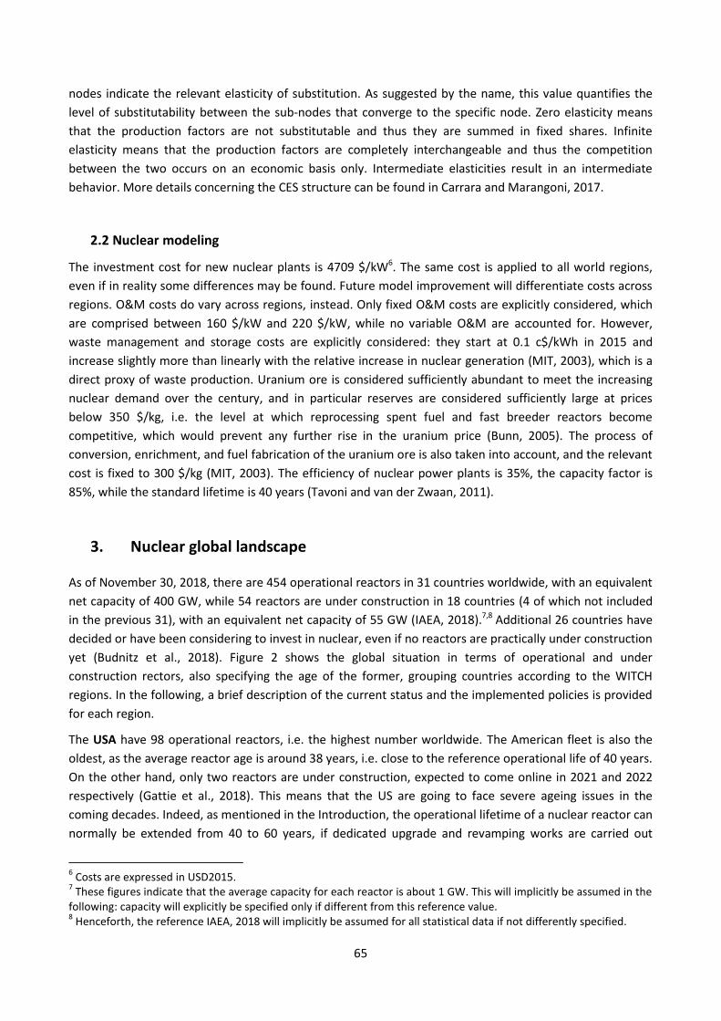
Similarly, nuclear is a power technology which could play a fundamental role in future climate change mitigation, but its actual prospects are awkward in many parts of the world, especially Europe, and more in general the OECD countries. In this area, in fact, many countries revised their development plans after the incident at the Fukushima power plant in 2011. At the same time, reactors have been ageing and a considerable number are approaching the end of their operational lifetime, therefore huge investments would be needed just to maintain the same generation level. In this perspective, this task aims at exploring the real prospects of nuclear, also trying to understand the economic and policy implications of neglecting this technology in addressing climate change.

A paper has been produced for each of these three topics. The present deliverable is essentially the collection of these three papers, attached in the next pages. The relevant titles are:

Exploring pathways of solar PV learning-by-doing in Integrated Assessment Models

The techno-economic effects of the delayed deployment of CCS technologies on climate change mitigation

Reactor ageing and phase-out policies: global and European prospects for nuclear power generation

5

Exploring pathways of solar PV learning-by-doing

in Integrated Assessment Models

Carrara S.1,2*, Bevione M.1,3, de Boer H.S.4, Gernaat D.4, Mima S.5, Pietzcker R.C.6, and Tavoni M.7,8,9

1 Fondazione Eni Enrico Mattei (FEEM), Milan, Italy 2 Renewable and Appropriate Energy Laboratory (RAEL), University of California, Berkeley, USA 3 INRIA, Grenoble, France 4 PBL Netherlands Environmental Assessment Agency, Den Haag, the Netherlands 5 CNRS - Université Grenoble Alpes, Grenoble, France 6 PIK Potsdam Institute for Climate Impact Research, Potsdam, Germany 7 European Institute on Economics and the Environment (EIEE), Milan, Italy 8 Centro Euro-Mediterraneo sui Cambiamenti Climatici (CMCC), Milan, Italy 9 Politecnico di Milano, Milan, Italy

*Corresponding author: samuel.carrara@feem.it

Abstract

The capital cost of solar photovoltaics (PV) has constantly decreased over the past decades, and market

competitiveness is not far now. The literature agrees in predicting further cost decrease in the future, even

if uncertainty remains on the actual path. Most importantly, it is unclear how reducing costs will translate

in actual PV penetration in the energy system in the long term. Integrated Assessment Models (IAMs)

generate low carbon transition scenarios, but typically assume exogenous learning and have not explored

future ranges of PV cost decline systematically. Here, we report from a multi-model comparison involving

four IAMs with a twofold objective: i) explore different PV capital cost pathways deriving from different

assumptions on endogenous learning-by-doing, and ii) assess the impacts that these low cost pathways

have on the penetration of PV and Variable Renewable Energies (VREs) in the electricity mix.

Results show that PV penetration in the electricity mix in the long-run (average over the period 2050-2100)

can range between 10-72% depending on the scenario, but that it is not very sensitive to capital cost, and

responds asymmetrically to learning rates. Sensitivity of PV penetration to capital cost reduction is

averagely 0.4 across scenarios. This highlights the importance of non-capital cost factors, most importantly

system integration, and the competition from alternative low carbon sources, including Carbon Capture

and Storage (CCS). The diffusion of PV crowds out other variable renewable energy such as wind and

concentrated solar power, resulting in lowered sensitivity of the penetration of VREs to PV costs. These

results point to the need to further evaluate how different low carbon alternatives interact when exploring

low carbon pathways.

6

Introduction

In 2015, the Paris Agreement marked the path for climate change mitigation in the coming decades

(Schellnhuber et al., 2016). Reaching ambitious mitigation goals compatible with the long-term target of

2°C requires an electrification of the energy sector and a parallel decarbonization of the electricity sector

(Creutzing et al. , 2017, Capros et al., 2012, and Wei et al., 2013). In this perspective, the importance of

solar photovoltaics (PV) as a power technology has rapidly grown in the last years, reaching 400 GW of

global installed capacity in 2017 (SolarPower, 2018), and according to virtually all studies it will play a major

role in the future energy scenario (Kriegler et al., 2014). One of the most important factors influencing PV

penetration in the electricity mix is its investment cost. This cost constantly decreased in the past and this

trend is expected to continue in the next decades (IEA, 2014 and Pietzcker et al., 2014). However,

substantial uncertainty still remains on the actual future cost evolution and on the consequent impacts on

PV penetration (Nelson et al., 2012 and Mileva et al., 2013). Indeed, models have regularly underestimated

the speed of cost decrease of solar PV (Luderer et al., 2017) and, more in general, its share in energy

projections (Creutzing et al. , 2017).

Integrated Assessment Models (IAMs) are widely used tools to explore future mitigation pathways and

capture in a coherent tool the different dimensions of climate change mitigation, involving energy,

economy, and the environment. In the past years, a consortium of European research teams participated in

the ADVANCE project (http://www.fp7-advance.eu/), aimed at developing new modeling solutions for

power sector dynamics, with a particular focus on the challenges of integrating solar and wind technologies

in the electricity system (Pietzcker et al., 2017). The multi-model exercise conducted in that context

highlighted once again the paramount role that Variable Renewable Energies (VREs, i.e. wind and solar),

and especially solar PV, will play in future power systems (Luderer et al., 2017).

The ADVANCE exercise carried out a sensitivity analysis on the most relevant parameters affecting VRE

diffusion (e.g. capital costs, resource availability), but did not perform any extensive analysis of the cost

patterns related to the technology learning process. Therefore the ADVANCE teams whose models have an

endogenous description of the capital cost evolution of power technologies decided to follow up the

exercise exploring the impacts of the different cost patterns on PV penetration in the electricity mix and on

other relevant variables. The main objective of this work is to explore different scenarios related to the

possible future endogenous cost patterns of the solar PV technology and the relevant impacts on the

electricity mix. To our knowledge, this is the first multi-model exercise exploring endogenous cost

pathways, whereas the several cost sensitivity analyses present in the literature, as well as the IPCC

reports, have always had an exogenous approach. Such an exercise also allows assessing the

responsiveness of models to changes in the cost data input. A review on the PV capital cost trends over the

last decades, and in particular on the learning rates which describe this trend, is also proposed.

Learning curves and learning rates

Integrated Assessment Models do not investigate the actual socio-technical dynamics that leads to cost

reductions. Rather, they try to identify simplified empirical correlations which are adopted to project future

patterns.The investment cost evolution for renewable power technologies in IAMs is often modeled

through an endogenous learning process, mainly described according to two schemes, which can be

applied singularly or jointly: learning-by-doing (LBD) and learning-by-researching (LBR). LBD relates the cost

decrease to the experience gained with deployment, while LBR describes the cost decrease as a

7

consequence of dedicated R&D investment. The vast majority of IAMs implement a one-factor learning

curve according to the LBD framework, see equation (1):

𝐶𝐶𝑡 = 𝐶𝐶1 (𝐾𝑡

𝐾1)−𝑏

(1)

where the ratio between the capital cost at time t (CCt) and the initial one (CC1) depends on the ratio

between the cumulative capacity at time t (Kt) and the initial one (K1) to the negative power of a parameter

(b), which measures the strength of the learning effect. It relates to the learning rate, LR, which measures

the rate at which unit costs decrease for each doubling of the cumulative capacity, through the following

relationship: LR = 1-2-b. Thus, a 20% learning rate means that technology costs fall by 20% when the

cumulative installed capacity doubles compared to the initial level.

Models normally include a floor cost (FC) to set a minimum price below which investment costs cannot fall.

The floor cost can either be applied as a hard bound or a soft bound. In the first case, no changes are

applied to the LBD formula and the cost is fixed to the floor cost once the threshold has been reached, see

equation (2):

𝐶𝐶𝑡 = 𝑚𝑎𝑥 {𝐹𝐶, 𝐶𝐶1 (𝐾𝑡

𝐾1)−𝑏

} (2)

In the second case, the floor cost identifies the “incompressible” portion of the initial cost which cannot

undergo learning (asymptotic formulation), see equation (3):

𝐶𝐶𝑡 = 𝐹𝐶 + (𝐶𝐶1 − 𝐹𝐶) ∙ (𝐾𝑡

𝐾1)−𝑏

(3)

In this configuration, the same learning rate generates a lower cost decrease with respect to the hard

bound formula.

IAMs rely on empirical evidence for the calibration of learning rate parameters. Several reviews have been

carried out of the existing empirical literature on historical learning rates for power generation

technologies, both in terms of LBD and in terms of LBR. Focusing on solar PV, Table SM-1 in the

Supplementary Material summarizes the estimates reported in the reviews carried out in the last decade

(Rubin et al., 2015, Baker et al. 2013, de La Tour et al. 2013, Junginger et al. 2008, Kahouli-Brahmi 2008,

Neij 2008) along with some new econometric analyses (Witajewski-Baltvilks et al. 2015, Lee 2012).

LBD estimates a cluster around 20% of cost reduction for each doubling in the cumulative installed

capacity, with a range from 9 to 47%. The broad range in estimates is due to the temporal and geographical

characteristics of the data set used in the estimation, the empirical specification, and the extent to which

endogeneity issues are addressed (Soderholm and Sundqvist 2007, Nordhaus 2009, Witajewski-Baltvilks et

al. 2015). Witajewski-Baltvilks et al. (2015) show how LBD rates can vary when statistical uncertainty is

considered and when some of the variables that are generally omitted from experience curves, such as

policies and energy prices, are included.

8

As discussed in Sagar and van der Zwaan (2006), it is not clear how learning rates should be extrapolated

when moving into the future. Soderholm and Sundqvist (2007) find that learning rate estimates over more

recent periods are larger than those calculated on the full sample because of the market power that

characterizes the initial diffusion of the technology, whereas the increased competition that emerged

during the diffusion stage led to a faster decline in technology costs. However, bias could also go in the

other direction because of diminishing returns and the difficulty of further reducing costs beyond certain

levels. Additionally, what has not been fully explored is how different learning rates interact with floor cost

used by some models to determine technology penetration. This is one point addressed in this work,

especially considering that no estimate refers to the soft bound formulation.

Only a few estimates are available in the literature for future periods. IEA (2014) and Neij (2008) provide an

estimate for LBD rates up to 2035 and 2050 respectively, whereas Verdolini et al. (2018) present a review

on recent expert elicitation exercises about future cost reduction stemming from different levels of R&D

expenditures, see Table SM-3. While LBR estimates tend to be lower than the few estimates reported in the

empirical literature, LBD rates are not very different from the ones estimated from historical data.

Involved models and scenario design

Four IAMs agreed to take part in this exercise: IMAGE, POLES, REMIND, and WITCH, see Table 1 and

Methods. Monetary values reported in Table 1 and in the rest of the paper are expressed in USD2015. All

participating models implement the learning-by-doing modeling scheme, and in particular the soft-bound

modeling scheme for the floor cost, with clear benefits in the exercise coherence.

IMAGE POLES REMIND WITCH

Model type Partial

equilibrium model

Partial equilibrium

model

General equilibrium model

General equilibrium model

Solution method Recursive dynamic

simulation

Recursive dynamic

simulation

Intertemporal optimization with perfect foresight

Intertemporal optimization with perfect foresight

Temporal horizon 2100 2100 2100 2100

PV cost calculation

Endogenous Endogenous Endogenous Endogenous

Type of endogenous

modeling

One-factor learning curve

(LbD)

One-factor learning curve

(LbD)

One-factor learning curve

(LbD)

One-factor learning curve

(LbD)

Regional differentiation

Yes, with (limited) spillover effects

on learning

No, only one global cost

No, only one global cost

No, only one global cost

Type of floor cost “Soft bound”

(asymptotic floor cost)

“Soft bound” (asymptotic floor

cost)

“Soft bound” (asymptotic floor

cost)

“Soft bound” (asymptotic floor

cost)

9

Plant depreciation

Linear Linear Concave Exponential

Depreciation rate 0.1 0.04 - 0.044

Lifetime [years] 25 25 30 25

Investment cost in 2015 [$/kW]

1576 1924 1916 1879

Learning rate 20% 15% 20% 20%

Floor cost [$/kW] 433 619 458 495

References de Boer and Van

Vuuren, 2017 Després et al.,

2017 Ueckerdt et al., 2017

Emmerling et al., 2016 and Carrara and Marangoni,

2017

Table 1 – Main features of the models participating in the exercise.

The exercise consists in a sensitivity analysis on the two main learning parameters: the learning rate and

the floor cost. In particular, a matrix of fourteen main cost scenarios is considered: seven learning rate

cases (reference and ±25%, ±50%, and ±75% with respect to reference) combined with two floor cost cases

(with and without floor cost).

The choice of the learning rate cases derives from an empirical estimate on the PV learning rate carried out

in the context of the ADVANCE project (Witajewski-Baltvilks et al., 2015) which identifies i) 19% as the

mean of the relevant normal distribution, and ii) the relative variations of ±25%, ±50%, and ±75% as the ±σ,

±2σ, and ±3σ values, respectively. The reference learning rate is meant to be the default one of the single

model. No harmonization efforts have been made across models, considering their calibration needs which

might lead to different choices within a reasonable range. Indeed, all models implement a learning rate of

20%, with the exception of POLES (15%).

The no floor cost case, especially if coupled with high learning rates, might well lead to an extreme

condition where the PV investment cost approaches zero. This is obviously a hardly policy-relevant

scenario, but it is useful to conduct diagnostic runs to check the behavior of models in such a configuration

and compare their outcome (Kriegler et al., 2015).

These scenarios are explored in a standard mitigation policy, where a carbon tax is applied in order to

achieve a long-term target of limiting the temperature increase in 2100 with respect to the pre-industrial

levels below 2°C with a likely chance, in line with the Paris targets. In detail, the tax starts in 2020 and is

calibrated so as to reach a global cumulative amount of CO2 emissions equal to 1000 Gt in the period 2011-

2100 in the reference scenario. The same tax is then applied to all the other mitigation scenarios. No

further sensitivity analysis is conducted on the policy dimension, since this aspect is not within the scope of

this work (in any case it has been thoroughly addressed in many other research works). A baseline case (no

10

policy) is added for benchmarking purposes, considering the two scenarios with and without floor cost. The

total is thus sixteen scenarios, detailed in Table SM-4.

Results

The set of explored learning rates produces a wide range of capital cost patterns throughout the century,

see Figure 1 (IMAGE reports the global average cost weighted on PV capacity in the different regions). This

range practically covers all the possible cost futures. All models show a robust behavior with this respect. In

the baseline case, costs span a range of 1057-1316 $/kW in 2050 and 571-1027 $/kW in 2100. In the

reference mitigation case, the range is 665-1156 $/kW in 2050 and 495-981 $/kW in 2100. In the most

pessimistic scenario (MIT-LR-75m-FC-ref) the range is 1467-1726 $/kW in 2050 and 1348-1512 $/kW in

2100, while in the most optimistic scenario (MIT-LR-75p-FC-0) the range is 53-273 $/kW in 2050 and

21-73 $/kW in 2100. The pessimistic scenario considers the hypothesis of essentially no cost decrease over

the century (the average cost decrease is only 20% across models), while the lower bound reached in the

optimistic scenario essentially corresponds to a null cost. Both configurations are unrealistic, but as already

noted it can be interesting to stress models in these extreme conditions.

Figure 1 – Global solar PV investment cost over time. Scenario names are defined as follows: policy (BASE =

baseline or MIT = mitigation), learning rate (ref = reference learning rate, 25m = ref-25%, 50m = ref-50%,

75m = ref-75%, 25p = ref+25%, 50p = ref+50%, 75p = ref+75%), floor cost (ref = reference floor cost, 0 = no

floor cost).

11

As predictable, the different cost pathways lead to very different PV penetration levels in the

corresponding scenarios. The interesting insight, however, is that comparable cost patterns lead to marked

differences across models. Figure 2 provides a more detailed overview of the average PV penetration over

the period 2050-2100 in the sixteen scenarios, dividing between the two cases with and without floor cost.

Average results in the 2050-2100 period are shown in order to discuss long-term trends without focusing

on any specific year. In general, scenarios without the floor cost show higher penetration than scenarios

where the reference floor cost is applied, as in the latter case the learning effect operates on a limited

portion of the initial cost and thus the cost decrease is faster. It is interesting to note that REMIND, which

shows the highest PV penetration levels, also shows the highest sensitivity to learning rates. In particular,

the average PV penetration in 2050-2100 in the reference mitigation scenarios is 53% with floor cost and

67% without floor cost, respectively. The range comprised between the LR-75m and LR-75p scenarios is 13-

62% with floor cost and 14-72% without floor cost (baseline scenarios are excluded from this account as

they are reported only as benchmarks). On the opposite side, not only is POLES the model generating the

lowest PV penetration levels, but it is also characterized by the lowest elasticity, especially in the scenarios

with floor cost. More in detail, PV penetration in the reference mitigation scenarios is 17% with floor cost

(with a range of 14-18%) and 20% without floor cost (with a range of 14-29%), respectively. IMAGE and

WITCH show intermediate and very similar results. In IMAGE, the average PV share is 16% in the reference

mitigation scenario with floor cost (range: 10-19%) and 27% without floor cost (range: 12-39%), while for

WITCH the corresponding results are 19% (range: 12-24%) and 26% (range: 13-35%), respectively.

Figure 2 – Global solar PV share in the electricity mix (average 2050-2100).

12

Three main insights can be drawn from these results. First, despite the huge differences in the explored

cost patterns, most models show a relatively modest sensitivity in terms of PV penetration. The most

evident case is given by POLES in the scenarios with floor cost: PV penetration is practically insensitive to

capital cost changes and remains restricted to a four-percentage point range. In this perspective, only

REMIND is a clear outlier, showing a huge sensitivity to capital costs. Second, even in the extreme cases

where PV can be installed practically for free, penetration does not reach particularly high levels, and in all

models except REMIND it remains well below 50%. Third, in all models and in both floor cost

configurations, PV penetrations show an asymmetric behavior, tending to collapse towards a sort of upper

bound: this means that models show higher sensitivity to lower learning rates than to higher learning rates.

This fact is highlighted in Figures SM-1 and SM-2 in the Supplementary Material, which explicitly show the

relative variation of PV penetration in the different learning rate scenarios centered on the reference case,

with and without floor cost, respectively.

Figure 3 provides a full overview of the PV penetration as a function of the relative cost reduction with

respect to 2015, in order to quantify the sensitivity of PV penetration to capital cost reductions.

Figure 3 – Global PV penetration: sensitivity to cost reduction (each point corresponds to one specific year,

independently of the scenario to which it belongs). The interpolating line starts from 0.01 on the y-axis as

this is the global PV penetration in 2015.

IMAGE POLES

REMIND WITCH

13

REMIND shows the highest sensitivity, being equal to 0.59 (every percentage point of cost decrease implies

an increase of 0.59% in PV penetration). The other three models show a similar sensitivity: IMAGE 0.34,

POLES 0.24, WITCH 0.29. The overall average is 0.40. Results are indeed quite different between the two

halves of the century, as shown in Figures SM-5 and SM-6. In the period 2015-2050, the average sensitivity

is 0.31 (IMAGE 0.20, POLES 0.19, REMIND 0.46, WITCH 0.24), while in the period 2050-2100 the average

sensitivity is 0.46 (IMAGE 0.39, POLES 0.28, REMIND 0.72, WITCH 0.33).

Models clearly show that with cost collapsing to zero (i.e. to a relative cost reduction equal to 1), PV

penetration is well far from 100%. Rather, a general accumulation towards a sort of boundary is found

(with the partial exception of IMAGE). This highlights the importance of non-capital cost factors, especially

system integration, and the competition with other low-carbon technologies in achieving mitigation

targets. In this perspective, however, it is important to note that the exercise is not focused on discussing

the feasibility or the implications of a fully-solar or fully-renewable electricity mix (see for instance the

debate in Jacobson et al., 2015 and Clack et al., 2017). It considers solar PV given its historical and projected

cost evolution, but the framework could be applied to any similar technology.

How are the different PV penetration levels reflected on the overall penetration of Variable Renewable

Energies? Figure 4 reports the average VRE penetration in 2050-2100 in the explored scenarios, replicating

the graph regarding PV penetration of Figure 2. It is noted that in this work, VREs comprise wind and both

solar technologies, i.e. PV and CSP (Concentrated Solar Power), coherently with Pietzcker et al., 2017.

Figure 4 – Global VRE share in the electricity mix (average 2050-2100).

14

With the partial exception of IMAGE, VRE penetration appears practically insensitive to the different PV

capital cost paths. This is observed both in terms of reduced distance between scenarios within each of the

two floor cost configurations and across the two floor cost configurations. Essentially, the higher/lower PV

penetration associated to the different capital cost patterns occurs to the detriment/benefit of wind and

CSP. In other words, wind and CSP almost completely compensate the variations related to PV. This result is

particularly remarkable in REMIND, which is characterized by a very strong sensitivity as far as the mere PV

share was concerned. If the floor cost is applied, this model shows a VRE penetration of 75% (range:

70-77%), while penetration is equal to 77% (range: 70-79%) if no floor cost is considered. A similar

sensitivity range characterizes WITCH: VRE penetration in the reference case is 56% (range: 53-58%) with

floor cost, while it is 59% (range: 53-63%). POLES shows practically no sensitivity: VRE penetration is

clustered in the range 46-47% with floor cost and in the range 46-48% without floor cost. As said, IMAGE is

the only model showing a significant residual sensitivity: in the scenarios with floor cost, indeed VRE

penetration does not vary markedly, being 30% in the reference case and showing a range of 26-33%.

Scenarios without floor cost have a higher dispersion, instead: the result in the reference case is 39%, while

the range is 27-49%.

This limited variability is clearly reflected in the relative variation of VRE penetration in the different

learning rate scenarios centered on the reference case which is shown in Figures SM-12 and SM-13.

Figure 5 – Global VRE penetration.

It is interesting to note that here a clear collapse towards a sort of upper boundary is observed in REMIND

only, see Figure 5. In fact in this model the VRE penetration monotonously grows over time and the broad

variability found in the first half of the century progressively disappears as VRE penetration converges to

about 83%. This result is in line with Luderer et al. (2017), which describes the main set of scenarios carried

out in the ADVANCE exercise mentioned at the beginning of this paper. That multi-model exercise explored,

among others, a scenario where the Levelized Cost Of Electricity (LCOE) of VREs was aligned with the

lowest among traditional technologies (typically coal), showing that VRE penetration even in this generous

case would not exceed 70-80% on average across models on average in the period 2050-2100. This result

15

highlighted that the integration challenges, i.e. the issues related to the non-negligible penetration of

variable power sources in the electricity grid, are of paramount importance and, in general, have an impact

which is comparable to direct technology costs. POLES too shows a monotonous behavior and a sort of

convergence towards an asymptotic value, even if this value is around 50%, well below the “integration

threshold” found in Luderer et al., 2017. As a consequence, the limited variability has to be explained with

“internal” modeling reasons. This also applies to WITCH, which does not show any clear boundary level: the

evolution of VRE penetration freely follows its path, with a mutual “exchange” of the PV, CSP, and wind

contributions depending on the PV cost pattern. The limited sensitivity shown by WITCH can be explained

with the Constant Elasticity of Substitution (CES) framework that characterizes this model. In a CES

structure, inputs are combined in a production function with a level of substitutability defined by the

relevant elasticity (in this case, inputs are the energy generation contributions from the different

technologies). Lower-than-infinite elasticities imply that the inputs are not linearly combined, i.e. they

cannot be considered completely substitutable. This framework is adopted in order to implicitly model

what in reality is experienced as preference for heterogeneity: with a fully-linear, unconstrained

framework, the energy system would be dominated by the cheapest technology, whereas in reality the

market is characterized by a plurality of choices, driven by a wealth of social, political, and technological

aspects which cannot fully be translated into simple economic constraints. Carrara and Marangoni (2017)

discuss the benefits of choosing an intermediate elasticity in the node combining the VRE and non-VRE

inputs in WITCH. Still, the CES structure is such that variations in one input (in our case, different levels of

PV generation derived from variable capital costs) have a primary impact on the closest CES nodes (hence,

wind and CSP) and only secondarily on the other technologies. Finally, in IMAGE the sensitivity increases

over time instead of diminishing. In this case, neither a real barrier due to the integration challenges nor

specific internal constraints seem to be present, allowing higher flexibility in response to the different PV

cost inputs.

It is finally interesting to analyze how the different PV and VRE penetration levels impact on the overall

electricity mix (Figure 6).

In the baseline scenario with floor cost, models project quite a similar global electricity demand averaged

over the period 2050-2100, comprised between 290 EJ/yr (IMAGE) and 343 EJ/yr (WITCH). To put these

numbers in perspective, this means about a threefold to fourfold increase from the 87 EJ/yr registered in

2015 (IEA, 2107). The no policy scenario results in a dominance of fossil-based plants in IMAGE: coal and

gas production sum up to 74% of the whole generation, while VREs are limited to 11%. On the other hand,

POLES and REMIND envisage a strong decarbonization even in the absence of mitigation policies: VREs

account for 45% and 42% of the electricity mix, respectively, even if with a prevalence of wind in POLES

(27%-18%), while solar – almost completely PV – prevails in REMIND (33%-9%). WITCH shows an

intermediate result: 25% of VRE penetration, with prevalence of wind (17%-8%).

Several research works have highlighted that the mitigation of greenhouse gas emissions can have opposite

effects on the electricity demand: if energy efficiency measures prevail, demand is likely to decrease with

respect to the baseline projections, whereas if a strong electrification of the energy sector coupled with a

decarbonization of the electricity sector prevails (especially based on renewables), demand is likely to

increase. The models involved in this exercise show quite a diverse behavior: focusing on the reference

mitigation case with floor cost (MIT-LR-ref-FC-ref), IMAGE shows the first trend (the average 2050-2100

global electricity demand decreases to 224 EJ/yr), REMIND shows the second trend (demand rises up to

423 EJ/yr), while the two effects tend to compensate in POLES (310 EJ/yr) and WITCH

(357 EJ/yr). Unsurprisingly, the electricity mix is dominated by VREs in REMIND (75%), while “centralized”

technologies, i.e. Carbon Capture and Storage (CCS), nuclear, and hydro have the lion’s share in IMAGE

16

(67%), with VREs accounting for 30% only. Intermediate results are found in POLES and WITCH, where VREs

account for 47% and 56% of the electricity mix, respectively (interestingly, in POLES it is about the same

level found in the baseline scenario).

Figure 6 – Electricity mix in selected scenarios (BASE-LR-ref-FC-ref, MIT-LR-ref-FC-ref, MIT-LR-75m-FC-ref,

MIT-LR-75p-FC-0).

Conclusions and discussion

This paper describes a multi-model exercise aimed at exploring different endogenous learning routes

applied to solar PV and their impacts on PV penetration in the electricity mix. The exercise involves four

Integrated Assessment Models which describe the cost evolution of solar PV according to a learning-by-

doing framework with floor cost. Scenarios are explored on a standard mitigation policy compatible with

the Paris targets and cover a wide variety of cost patterns compatible with any reasonable cost futures.

Global PV penetration in the long run (in particular, averaging over the 2050-2100 period) spans a range of

10-72%, with a marked growth with respect to the current 1% in all scenarios and models. Despite the

marked variation of costs and the variability observed across models, all models tend to show a limited

sensitivity to PV penetration in their specific results. Sensitivity of PV penetration to capital cost reduction

is averagely 0.4 across scenarios, being lower in the first half of the century (0.31) than in the second half

(0.46). Sensitivity is not symmetric with respect to increasing or decreasing learning rates, being markedly

higher for the latter. Indeed, all models tend to show a sort of “threshold” on which PV penetration tends

to collapse even in the most favorable scenarios. This highlights the role of non-capital cost factors,

17

especially system integration, and the competition with alternative low carbon sources, including Carbon

Capture and Storage. In this regard, it is reminded that it is not within the scope of this work to discuss the

feasibility or the implications of reaching a fully-solar or fully-renewable electricity portfolio. Sensitivity to

PV capital cost even diminishes when all variable renewable energies (i.e. wind and solar CSP in addition to

PV) are focused. This means that, according to the models participating in this exercise, competition of

solar PV takes place primarily with wind and CSP, and the higher/lower penetration related to lower/higher

capital costs mainly occurs to the detriment/benefit of these technologies. This is partly explained with

modeling reasons (e.g. the role of the Constant Elasticity of Substitution framework in the WITCH model),

but also suggests the need for further research concerning the competition within variable renewable

energies, and between them and the other power technologies, which indeed is not within the scope of

this work.

Acknowledgments

This project has received funding from the European Union's Horizon 2020 research and innovation

programme under the Marie Sklodowska-Curie grant agreement No 706330 (MERCURY).

The research leading to these results has received funding from the European Union’s Seventh Framework

Programme [FP7/2007-2013] under grant agreement n° 308329 (ADVANCE).

References

1. Baker et al. (2013). The Economics of Solar Electricity, Annual Review of Resource Economics,

Vol. 5, pp. 387-426.

2. Capros, P., Tasios, N., De Vita, A., Mantzos, L., and Proussos, L. (2012). Transformations of the

energy system in the context of the decarbonisation of the EU economy in the time horizon to

2050. Energy Strategy Reviews, 1(2), 85-96.

3. Carrara S. and Marangoni G. (2017), Including system integration of Variable Renewable

Energies in a Constant Elasticity of Substitution framework: the case of the WITCH model,

Energy Economics, Vol. 64, pp. 612-626

4. Clack, C.T.M., Qvist, S.A., Apt, J., Bazilian, M., Brandt, A.R., Caldeira, K., Davis, S.J., Diakov, V.,

Handschy, M.A., Hines, P.D.H., Jaramillo, P., Kammen, D.M., Long, J.C.S., Granger Morgan, M.,

Reed, A., Sivaram, V., Sweeney, J., Tynan, G.R., Victor, D.G., Weyant, J.P., and Whitacre, J.F.

(2017), Evaluation of a proposal for reliable low-cost grid power with 100% wind, water, and

solar, PNAS – Proceedings of the National Academy of Sciences, Vol. 114, N. 26, pp. 6722-6727

5. Creutzig, F., Agoston, P., Goldschmidt, P.J., Luderer, G., Nemet, G., Pietzcker, R.C. (2017) The

underestimated potential of solar energy to mitigate climate change, Nature Energy 2, 17140

6. de Boer H.S. and van Vuuren D.P. (2017), Representation of variable renewable energy sources

in TIMER, an aggregated energy system simulation model, Energy Economics, Vol. 64, pp. 600-

611

7. de La Tour, A., Glachant, M., and Ménière, Y. (2013). Predicting the costs of photovoltaic solar

modules in 2020 using experience curve models, Energy, Vol. 62, pp. 341-348.

18

8. Després J., Mima S., Kitous A., Criqui P., Hadjsaid N. and Noirot I. (2017), Storage as a flexibility

option in power systems with high shares of variable renewable energy sources: a POLES-based

analysis, Energy Economics, Vol. 64, pp. 638-650

9. Emmerling, J., L. Drouet, L. A. Reis, M. Bevione, L. Berger, V. Bosetti, S. Carrara, E. De Cian, G.

De Maere D'Aertrycke, T. Longden, M. Malpede, G. Marangoni, F. Sferra, M. Tavoni, J.

Witajewski-Baltvilks, P. Havlik, (2016), The WITCH 2016 Model - Documentation and

Implementation of the Shared Socioeconomic Pathways, FEEM Working Paper 042.2016

10. IEA, International Energy Agency (2014). Technology Roadmap: Solar Photovoltaic Energy

11. IEA, International Energy Agency (2017). World Energy Outlook 2017

12. Jacobson, M.Z., Delucchi, M.A., Cameron, M.A., and Frewa B.A. (2015). Low-cost solution to the

grid reliability problem with 100% penetration of intermittent wind, water, and solar for all

purposes, PNAS – Proceedings of the National Academy of Sciences, Vol. 112, No. 49,

pp. 15060-15065

13. Junginger, H. M., Lako, P., Lensink, S., van Sark, W. G. J. H. M., and Weiss, M. (2008).

Technological learning in the energy sector.

14. Kahouli-Brahmi, S. (2008). Technological learning in energy–environment–economy modelling:

A survey. Energy Policy, Vol. 36, pp. 138-162.

15. Kriegler, E.,Weyant, J.P., Blanford, G.J., Krey, V., Clarke, L., Edmonds, J., Fawcett, A., Luderer, G.,

Riahi, K., Richels, R., Rose, S.K., Tavoni, M., van Vuuren, D.P. (2014). The role of technology for

achieving climate policy objectives: overview of the EMF 27 study on global technology and

climate policy strategies. Climatic Change 123, 353-367

16. Kriegler, E., Petermann, N., Krey, V., Schwanitz, V.J., Luderer, G., Ashina, S., Bosetti, V., Eom, J.,

Kitous, A., Méjean, A., Paroussos, L., Sano, F., Turton, H., Wilson, C., and van Vuuren D.P. (2015).

Diagnostic indicators for integrated assessment models of climate policy. Technological

Forecasting and Social Change 90A, 45-61.

17. Lee, Y. (2012). Learning-by-doing effect from solar photovoltaic RD&D. Conference proceeding

of the 3rd IAEE Asian Conference, Kyoto, Japan.

18. Luderer, G., Pietzcker, R.C., Carrara, S., de Boer, H.S., Fujimori, S., Johnson, N., Mima, S., Arent,

D. (2017). Assessment of wind and solar power in global low-carbon energy scenarios: An

introduction. Energy Economics 64, 542-551.

19. Mileva, A., Nelson, J. H., Johnston, J. & Kammen, D. M. (2013). SunShot solar power reduces

costs and uncertainty in future low-carbon electricity systems. Environmental Science &

Technology, 47, 9053-9060

20. Neij, L. (2008). Cost development of future technologies for power generation—a study based

on experience curves and complementary bottom-up assessments, Energy Policy, Vol. 36,

pp. 2200-2211.

21. Nelson, J., Johnston, J., Mileva, A., Fripp, M., Hoffman, I., Petros-Good, A., Blanco, C., Kammen,

D.M. (2012). High-resolution modeling of the western North American power system

demonstrates low-cost and low-carbon futures, Energy Policy, 43, 436-447

19

22. Nordhaus, W. D. (2009). The perils of the learning model for modeling endogenous

technological change (No. w14638). National Bureau of Economic Research.

23. Pietzcker, R.C., Stetter, D., Manger, S., Luderer, G. (2014). Using the sun to decarbonize the

power sector: the economic potential of photovoltaics and concentrating solar power. Applied

Energy 135, 704-720.

24. Pietzcker, R.C., Ueckerdt, F., Carrara, S., de Boer, H.S., Després, J., Fujimori, S., Johnson, N.,

Kitous, A., Scholz, Y., Sullivan, P., Luderer, G., 2017. System integration of wind and solar power

in integrated assessment models: a cross-model evaluation of new approaches. Energy

Economics 64, 583-599.

25. Rubin, E. S., Azevedo, I. M., Jaramillo, P., and Yeh, S. (2015). A review of learning rates for

electricity supply technologies. Energy Policy, 86, 198-218.

26. Sagar, A. D. and Van der Zwaan, B. (2006). Technological innovation in the energy sector: R&D,

deployment, and learning-by-doing, Energy Policy, Vol. 34, pp. 2601-2608.

27. Schellnhuber, H. J., Rahmstof, R. &Winkelmann, R. (2016) Why the right climate target was

agreed in Paris. Nature Climate Change 6, 649-653.

28. Söderholm, P. and Sundqvist, T. (2007). Empirical challenges in the use of learning curves for

assessing the economic prospects of renewable energy technologies, Renewable Energy, Vol.

32, pp. 2559-2578.

29. SolarPower (2018), Global market outlook for solar power 2018-2022

30. Ueckerdt F., Pietzcker R.C., Scholz Y., Stetter D., Giannousakis A. and Luderer G. (2017).

Decarbonizing global power supply under region-specific consideration of challenges and

options of integrating variable renewables in the REMIND model, Energy Economics, Vol. 64, pp.

665-684

31. Verdolini, E., Díaz Anadón, L., Baker, E., Bosetti, V., and Aleluia Reis, L. (2018). Future Prospects

for Energy Technologies: Insights from Expert Elicitations, Review of Environmental Economics

and Policy, Vol. 12, pp. 133–153

32. Wei, M., Nelson, J.H., Greenblatt, J.B., Mileva, A., Jonhston, J., Ting, M., Yang, C., Jones, C.,

McMahon, J.E., and Kammen D.M. (2013). Deep carbon reductions in California require

electrification and integration across economic sectors, Environmental Research Letters, 8(1),

014038

33. Witajewski-Baltvilks J., Verdolini E. and Tavoni M. (2015), Bending the learning curve, Energy

Economics, Vol. 52, pp. S86-S99

20

Exploring pathways of solar PV learning-by-doing

in Integrated Assessment Models – Supplementary Material

Carrara S.1,2*, Bevione M.1,3, de Boer H.S.4, Gernaat D.4, Mima S.5, Pietzcker R.C.6, and Tavoni M.7,8,9

1 Fondazione Eni Enrico Mattei (FEEM), Milan, Italy 2 Renewable and Appropriate Energy Laboratory (RAEL), University of California, Berkeley, USA 3 INRIA, Grenoble, France 4 PBL Netherlands Environmental Assessment Agency, Den Haag, the Netherlands 5 CNRS - Université Grenoble Alpes, Grenoble, France 6 PIK Potsdam Institute for Climate Impact Research, Potsdam, Germany 7 European Institute on Economics and the Environment (EIEE), Milan, Italy 8 Centro Euro-Mediterraneo sui Cambiamenti Climatici (CMCC), Milan, Italy 9 Politecnico di Milano, Milan, Italy

*Corresponding author: samuel.carrara@feem.it

21

Learning-by-doing in solar PV: evidence from the existing literature

Soderholm and Sundqvist (2007) show that explicitly accounting for economies of scales reduces learning-

by-doing (LBD) rates, suggesting that if this driver is not modelled, LBD rates are upward biased. Soderholm

and Sundqvist (2007) show that including a time trend so as to capture any underlying change in trend

other than R&D knowledge stock or installed capacity absorbs all variation otherwise captured by the R&D

stock, whereas LBD rates are quite stable, especially when endogeneity issues are taken into account.

Most IAMs use an approach based on endogenous technological change modelled through a one-factor

learning curve (LBD) as described in equations (1) and (2). This is the case for E3MG, IMACLIM, IMAGE-

TIMER, REMIND and WITCH. A few models (MERGE-ETL, POLES – but not in the version adopted in this

work) use a two-factor learning curve for endogenous technological change, considering both the effects of

learning-by-doing and learning-by-researching, whereas some other models (e.g. MESSAGE and GCAM) use

an exogenous technical change by defining different investment costs for future periods (which vary

according to reference/policy scenarios). Table SM-2 summarizes the learning rates and the floor costs

used by the IAMs with endogenous technological change. Since models rely on empirical literature, it is not

surprising that the range of LBD rates in terms of minimum, maximum and mean values is similar to the

range emerging from the empirical literature in Table SM-1.

Source # Factors Rate LR (%) Timeframe Method

min max mean

Baker et al. (2013) 1 LBD 17 35 20 na Review

Junginger et al. (2008) 1 LBD 10 47 22 1957-2006 Review

Kahouli-Brahmi (2008) 1 LBD 18 35 23 1959-1998 Review

La Tour et al. (2013) 1 LBD 10 30 21 1965-2005 Review

Lee, conference proceeding

(2012) 2 LBR 9 15 11 2001-2010 Regression analysis

Lee, conference proceeding

(2012) 2 LBD 10 10 10 2001-2010 Regression analysis

Neij (2008) 1 LBD 10 47 20 1976-2001 Review

Rubin et al. (2015) 1 LBD 10 47 23 1959-2011 Review

Rubin et al. (2015) 2 LBR 10 14 12 1971-2001 Review

Rubin et al. (2015) 2 LBD 14 32 18 1971-2000 Review

Witajewski-Baltvilks et al.

2015, Mod 1 1 LBD 9 33 20 1990-2012 Regression analysis

Witajewski-Baltvilks et al.

2015, Mod 2 1 LBD 10 46 27 1990-2012 Regression analysis

22

Witajewski-Baltvilks et al.

2015, Mod 3 1 LBD 10 29 19 1990-2012 Regression analysis

Witajewski-Baltvilks et al.

2015, OLS 1 LBD 10 14 12 1990-2012 Regression analysis

Table SM-1: Learning rate estimates based on the empirical evidence.

Source # Factors Type LR (%) Timeframe Floor cost

min max mean

(2015$/k

W)

E3MG (Edenhofer et al. 2010) 1 LBD na na 30 Constant 1546

IMACLIM (Bibas et al. 2012)

central station PV

1

LBD

15

25

na

Constant

1215

rooftop PV 1 LBD 15 25 na Constant 2121

IMAGE-TIMER (Baker et al.

2013) 1 LBD na na 35 2000 0

1 LBD na na 9 2100 0

MERGE-ETL (Magné et al. 2010) 2 LBD na na 10 Constant 0

2 LBR na na 10 Constant 0

POLES (Criqui et al. 2015) 2 LBD na na 20 2010 1361

2 LBR na na 45 2010 1361

REMIND (Luderer et al. 2015) 1 LBD na na 20 Constant 619

WITCH (Emmerling et al., 2016) 1 LBD na na 16.5 Constant 619

Table SM-2: Learning rates and floor costs in IAMs. Miminum, maximum, and mean values for LR result

from the survey of existing models with endogenous technological change. “Constant” means that the LR is

constant over time, whereas in the other cases LR is varying over time and values for 2000/2010/2100 are

provided.

23

Source #

Factors

Rate R&D LR (%) Timefram

e

Method

Level min ma

x

mea

n

Bosetti et al. (2016)

CMU

1 LBR High -1 13 6 Future:

2030

Expert

elicitation

Bosetti et al. (2016)

FEEM

1 LBR High 4 12 7 Future:

2030

Expert

elicitation

Bosetti et al. (2016)

Harvard

1 LBR High -3 11 3 Future:

2030

Expert

elicitation

Bosetti et al. (2016)

CMU

1 LBR Low -2 13 5 Future:

2030

Expert

elicitation

Bosetti et al. (2016)

FEEM

1 LBR Low 1 10 6 Future:

2030

Expert

elicitation

Bosetti et al. (2016)

Harvard

1 LBR Low -2 8 2 Future:

2030

Expert

elicitation

Bosetti et al. (2016)

UMass

1 LBR Low -1 7 4 Future:

2030

Expert

elicitation

Bosetti et al. (2016)

FEEM

1 LBR Mid 2 11 6 Future:

2030

Expert

elicitation

Bosetti et al. (2016)

Harvard

1 LBR Mid -1 10 3 Future:

2030

Expert

elicitation

Bosetti et al. (2016)

UMass

1 LBR Mid -1 7 5 Future:

2030

Expert

elicitation

Neij (2008) 1 LBD - 15 25 20 Future:

2050

Expert

elicitation /

Extrapolation

from

historical

values

OECD/IEA (2014) 1 LBD - 20 20 20 Future:

2035

Extrapolation

from

historical

values

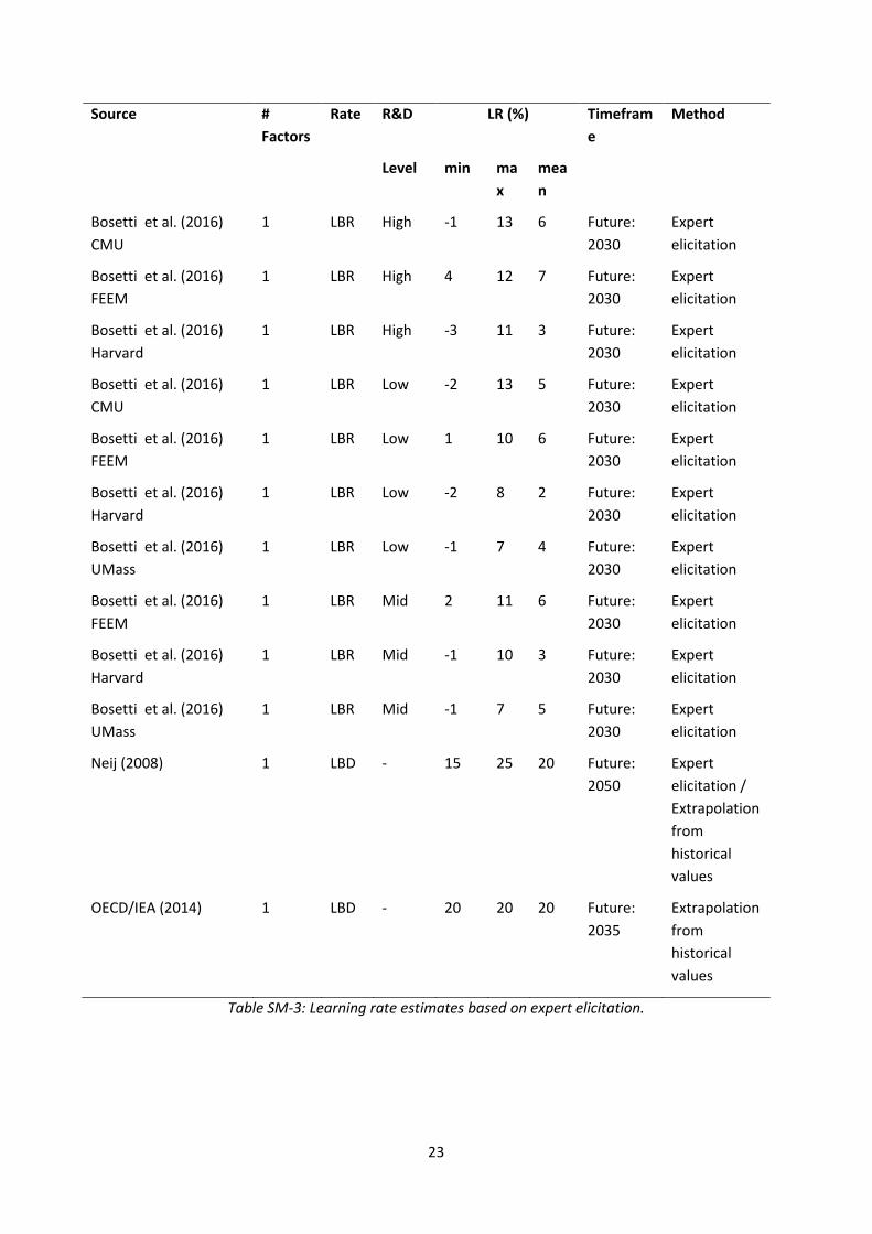
Table SM-3: Learning rate estimates based on expert elicitation.

24

Scenario matrix

Scenario Name Policy Learning Rate Floor Cost

1 BASE-LR-ref-FC-ref Baseline Ref Ref

2 BASE-LR-ref-FC-0 Baseline Ref 0

3 MIT-LR-75p-FC-ref Mitigation +75% Ref

4 MIT-LR-50p-FC-ref Mitigation +50% Ref

5 MIT-LR-25p-FC-ref Mitigation +25% Ref

6 MIT-LR-ref-FC-ref Mitigation Ref Ref

7 MIT-LR-25m-FC-ref Mitigation -25% Ref

8 MIT-LR-50m-FC-ref Mitigation -50% Ref

9 MIT-LR-75m-FC-ref Mitigation -75% Ref

10 MIT-LR-75p-FC-0 Mitigation +75% 0

11 MIT-LR-50p-FC-0 Mitigation +50% 0

12 MIT-LR-25p-FC-0 Mitigation +25% 0

13 MIT-LR-ref-FC-0 Mitigation Ref 0

14 MIT-LR-25m-FC-0 Mitigation -25% 0

15 MIT-LR-50m-FC-0 Mitigation -50% 0

16 MIT-LR-75m-FC-0 Mitigation -75% 0

Table SM-4 – Scenario set.

25

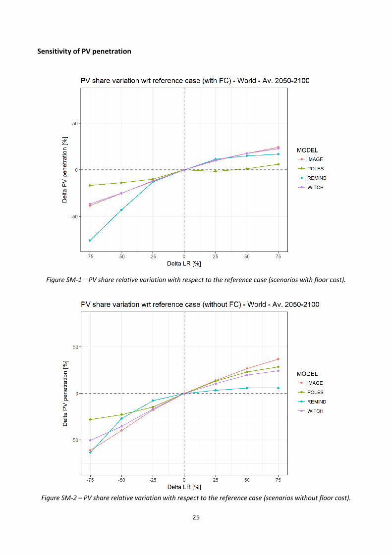
Sensitivity of PV penetration

Figure SM-1 – PV share relative variation with respect to the reference case (scenarios with floor cost).

Figure SM-2 – PV share relative variation with respect to the reference case (scenarios without floor cost).

26

Sensitivity of PV penetration to capital cost reduction

Figure SM-3 – Global PV penetration: sensitivity to cost reduction (all models).

Figure SM-4 – Global PV penetration: sensitivity to cost reduction (each point corresponds to one specific

year, independently of the scenario to which it belongs). Cost reductions are expressed as the ratio between

the capital cost in 2015 and the capital cost in the relevant year.

27

Figure SM-5 – Global PV penetration: sensitivity to cost reduction (2015-2050).

Figure SM-6 – Global PV penetration: sensitivity to cost reduction (2050-2100).

IMAGE

REMIND WITCH

POLES

IMAGE

REMIND WITCH

POLES

28

Figure SM-7 – Global PV penetration: sensitivity to cost reduction (2015-2050, all models).

Figure SM-8 – Global PV penetration: sensitivity to cost reduction (2050-2100, all models).

29

“Statistical” PV penetration

As discussed in the main text, Witajewski-Baltvilks et al. (2015) provide an empirical estimate of the PV

learning rate, not only in terms of mean value (19%) but in terms of statistical normal distribution, where

the relative variations of ±25%, ±50%, and ±75% correspond to the ±σ, ±2σ, and ±3σ values, respectively.

These values allow deriving the statistically average PV penetration shares, weighting the shares associated

to the different learning rates on the relevant values of the normal distribution, schematized in

Figure SM-9. The weights of the normal distribution corresponding to the median and the ±σ, ±2σ, and ±3σ

levels are 0.3989, 0.2420, 0.0540, and 0.0044, respectively.

Figure SM-9 – Normal probability density function.

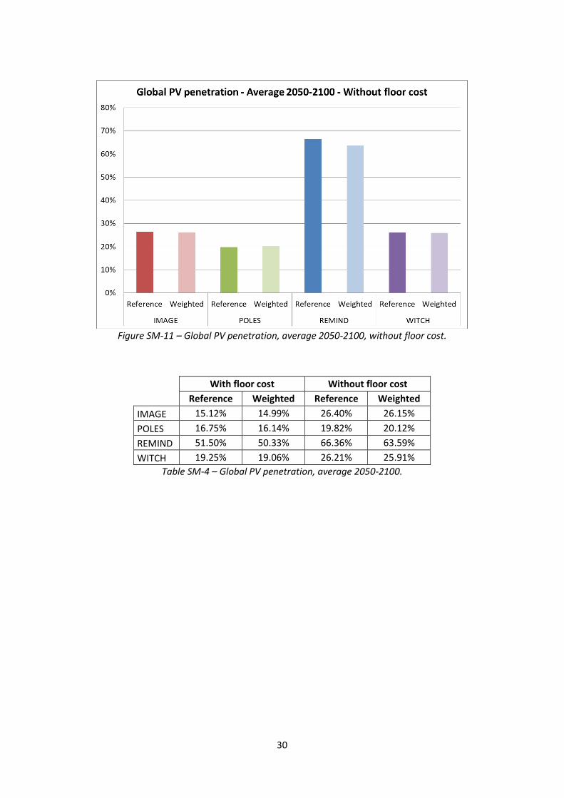
Figures SM-10 and SM-11 show the comparison between the average PV penetration in 2050-2100 in the

reference mitigation scenario and the penetration rate obtained with the statistical average, for both

configurations with and without floor cost, respectively. As noted in Figure 2 in the main text, models show

higher sensitivity to low learning rates, therefore the statistical average penetration rate is lower than the

reference one, apart from POLES in the scenarios without floor cost. Indeed, differences are not particularly

broad, with the partial exception of REMIND (see Table SM-4).

Figure SM-10 – Global PV penetration, average 2050-2100, with floor cost.

30

Figure SM-11 – Global PV penetration, average 2050-2100, without floor cost.

With floor cost Without floor cost

Reference Weighted Reference Weighted

IMAGE 15.12% 14.99% 26.40% 26.15%

POLES 16.75% 16.14% 19.82% 20.12%

REMIND 51.50% 50.33% 66.36% 63.59%

WITCH 19.25% 19.06% 26.21% 25.91%

Table SM-4 – Global PV penetration, average 2050-2100.

31

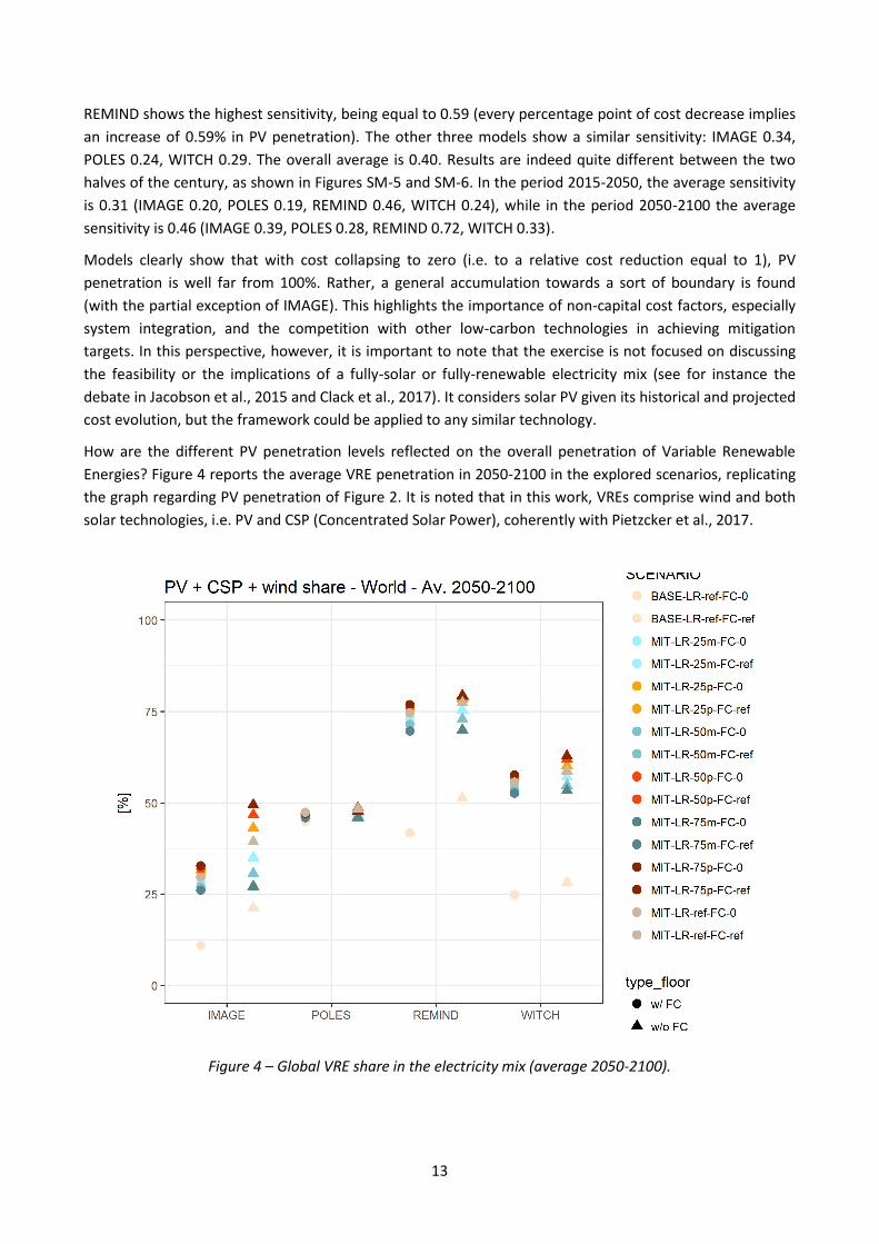
Sensitivity of VRE penetration

Figure SM-12 – VRE share relative variation with respect to the reference case (scenarios with floor cost).

Figure SM-13 – VRE share relative variation with respect to the reference case (scenarios without floor cost).

32

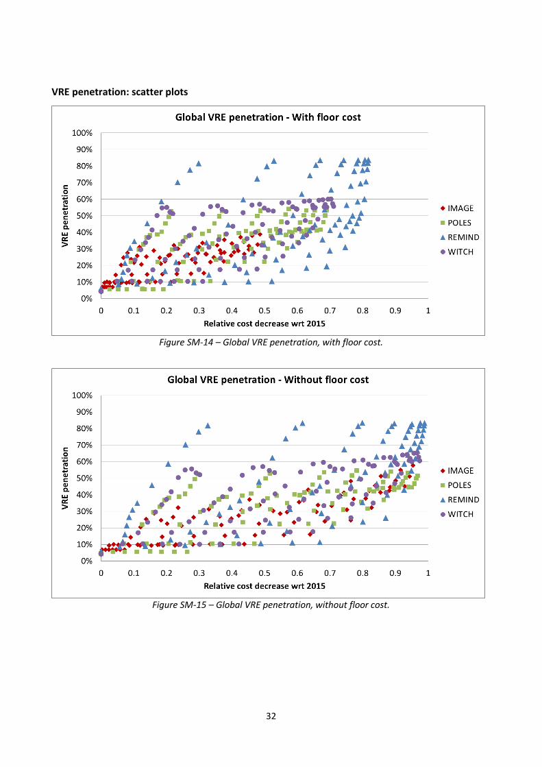
VRE penetration: scatter plots

Figure SM-14 – Global VRE penetration, with floor cost.

Figure SM-15 – Global VRE penetration, without floor cost.

33

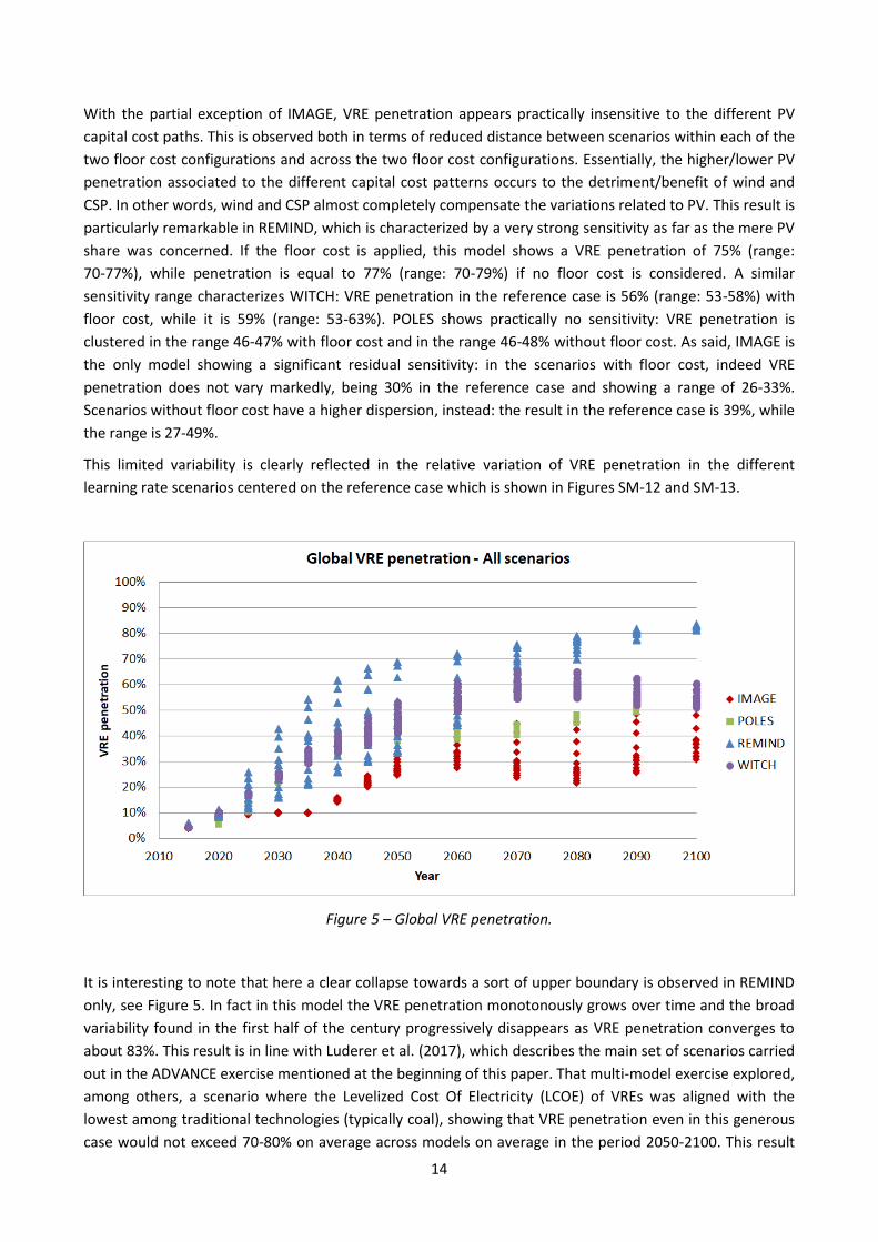
Figure SM-16 – Global VRE penetration, all scenarios.

Electricity mix

Figure SM-17 – Global electricity mix in selected years (Baseline scenario).

34

Figure SM-18 – Global electricity mix in selected years (Reference scenario).

Figure SM-19 – Global electricity mix in selected years (Optimistic scenario).

35

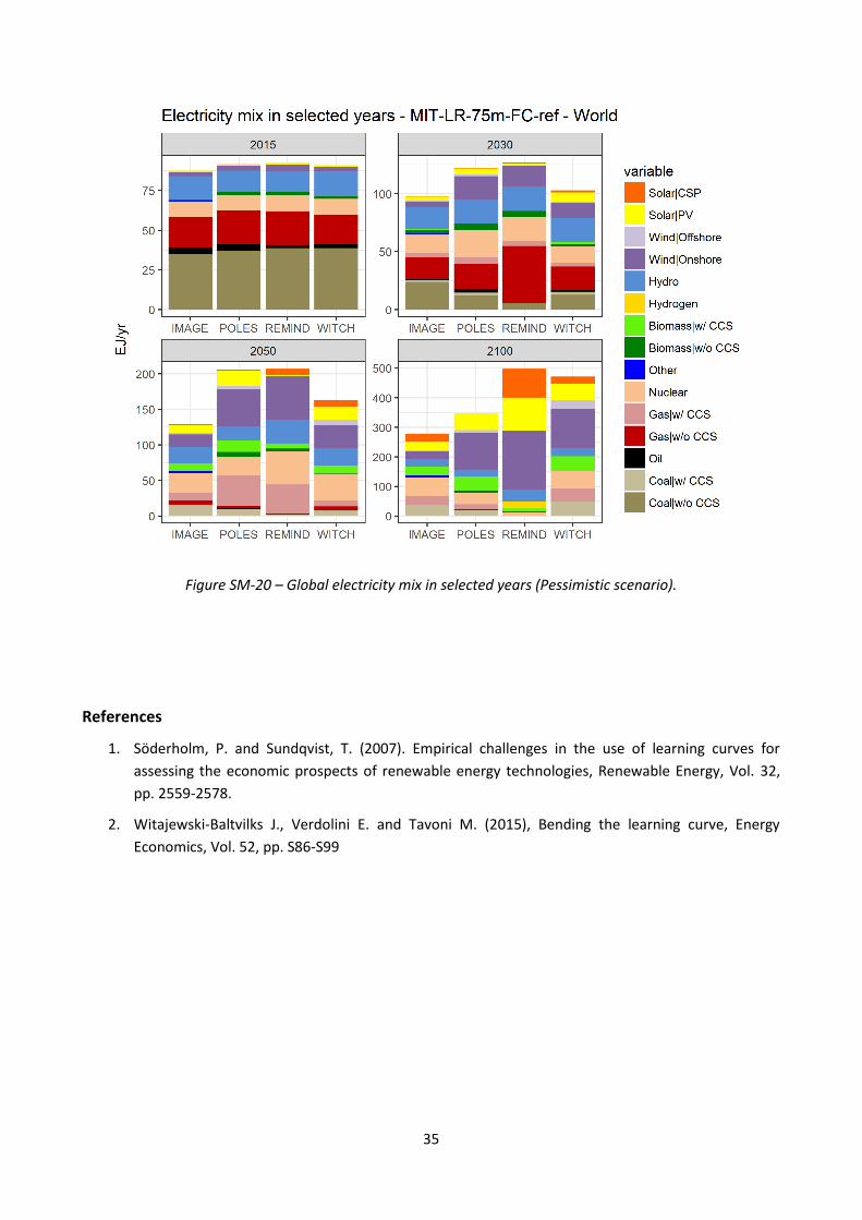
Figure SM-20 – Global electricity mix in selected years (Pessimistic scenario).

References

1. Söderholm, P. and Sundqvist, T. (2007). Empirical challenges in the use of learning curves for

assessing the economic prospects of renewable energy technologies, Renewable Energy, Vol. 32,

pp. 2559-2578.

2. Witajewski-Baltvilks J., Verdolini E. and Tavoni M. (2015), Bending the learning curve, Energy

Economics, Vol. 52, pp. S86-S99

36

The techno-economic effects of the delayed deployment of CCS technologies

on climate change mitigation

Samuel Carrara1,2*

1 Fondazione Eni Enrico Mattei (FEEM), Milan, Italy 2 Renewable and Appropriate Energy Laboratory (RAEL), University of California, Berkeley, USA

DRAFT COPY – DO NOT CITE

Abstract

Meeting the targets of climate change mitigation set by the Paris Agreement entails a huge transformation

of the energy sector, as low- or no-carbon technologies are predicted to gradually substitute traditional,

fossil-based technologies. In this perspective, the vast majority of energy scenarios project a fundamental

role of Carbon Capture & Storage (CCS). However, uncertainty remains on the actual techno-economic

feasibility of this technology: despite the considerable investment over the recent past, commercial

maturity is yet to come.

The main aim of this work is to evaluate the impacts of a progressively delayed deployment of CCS plants

from a climate, energy, and economic perspective, focusing in particular on the power sector. This is done

with the Integrated Assessment Model WITCH, exploring a wide set of long-term scenarios over mitigation

targets ranging from 1.5°C to 4°C in terms of temperature increase with respect to the pre-industrial levels.

The analysis shows that CCS will be a key mitigation option at a global level for carbon mitigation, achieving

about 30% of the electricity mix in 2100 (with a homogeneous distribution across coal, gas, and biomass) if

its deployment is unconstrained. If CCS deployment is delayed or forbidden, penetration cannot reach the

optimal unconstrained level, resulting in a mix rearrangement, with a strong increase in renewables and, to

a lesser extent, nuclear. The mitigation targets can be met, but policy costs are 35% to 72% higher without

the implementation of CCS than in the corresponding unconstrained scenarios. In Europe, CCS is not

projected to be a considerable mitigation option, therefore the sensitivity analysis over the mitigation

targets and the CCS deployment years does not highlight meaningful technical and economic changes.

Keywords: carbon capture and storage, power generation, climate change mitigation, Integrated

Assessment Models

____________________________

* Dr. Samuel Carrara, Researcher and Marie Skłodowska-Curie Fellow, Fondazione Eni Enrico Mattei (FEEM), Corso Magenta 63, 20123 Milan, Italy. Tel: +39-02-52036932, Fax: +39-02-52036946, E-mail: samuel.carrara@feem.it. This project has received funding from the European Union's Horizon 2020 research and innovation programme under the Marie Sklodowska-Curie grant agreement No 706330 (MERCURY).

37

1. Introduction

Climate change mitigation is acknowledged as one of the major challenges that the mankind will have to

face in the 21st century (IPCC, 2014). With the Paris Agreement, reached in 2015 during the Conference of

Parties 21 (COP21), almost all countries of the world have committed to pursuing the ambitious target of

limiting to 2°C the global temperature increase in 2100 with respect to the pre-industrial levels, making all

the possible efforts to stay as close to 1.5°C as possible, in order to further limit detrimental climate

impacts (Schellnhuber et al., 2016). However, these targets are very difficult to be reached, as they entail

huge technological and economical fundamental transformations, as well as an internationally coordinated

action.

Carbon Capture & Storage (CCS) has widely been recognized as one of the main technological solutions to

decarbonize the energy sector and virtually all research studies project a considerable role in future

mitigation pathways (Krey et al., 2014 and Koelbl et al., 2014), especially if the target is to stay below 2°C

(Rogelj et al., 2015). This technology consists in capturing the carbon dioxide generated in plants fed with

fossil fuels or biomass and storing it in proper underground deposits or marine aquifers (IEA, 2013). Its

main advantage is the possibility to achieve a (theoretically) zero carbon energy generation adopting fossil

fuels plants, i.e. without massively reconsidering the current generation paradigm that still dominates the

energy sector (IEA, 2017). Indeed, even negative emissions can be achieved if CCS plants are fed with

biomass which is replaced at a pace equal to consumption: in this case, the carbon neutrality related to the

use of biomass (net of the emissions associated to the whole life cycle concerning harvesting, transport

etc.) is complemented by the CO2 removal in the CCS plant. An additional advantage is related to the

dispatchability of these plants, which is a fundamental aspect in a future energy scenario where non-

dispatchable renewables (primarily wind and solar) will likely reach significant shares in the electricity mix.

CCS availability would also entail economic savings in pursuing mitigation targets (Davidson et al., 2017).

However, large-scale CCS deployment is yet to come. Safety concerning the stability of storage sites, public

acceptance, high technology costs, incomplete or unclear regulatory framework, the absence of business

models, and a general uncertainty on the socio-economic impacts are major obstacles that still hinder the

take-off of this technology (Creutzig et al., 2013 and Muratori et al., 2016). As a result, so far, very few and

small scale plants have been installed worldwide (GCCSI, 2017).

In this context, the main objective of this work is to investigate the role that CCS could play in carbon

mitigation and in particular assess the techno-economic impacts that a progressively delayed deployment

of this technology can have both in terms of re-arrangement of the energy mix and in terms of policy costs.

In other words, how urgent is it to start installing CCS plants for the feasibility of more and more stringent

climate targets?

This work focuses on the electricity sector, which is described in detail in the model adopted in this work,

the Integrated Assessment Model (IAM) WITCH.

The paper is structured as follows. Section 2 describes the WITCH model, and especially how CCS

technologies are modeled therein. Section 3 reports the scenario design. Section 4 reports and extensively

discusses the most relevant results of the analysis. Finally, Section 5 concludes.

38

2. Methodology

2.1 The WITCH model

The tool adopted in this research is the World Induced Technical Change Hybrid (WITCH) model. WITCH is a

dynamic optimization Integrated Assessment Model (IAM) designed to investigate the socio-economic

impacts of climate change over the 21st century (Bosetti et al., 2006 and Emmerling et al., 2016). It

combines a top-down, simplified representation of the global economy with a bottom-up, detailed

description of the energy sector, nested in a Constant Elasticity of Substitution (CES) structure

(Figure 1). The model is defined on a global scale: countries are grouped into thirteen aggregated regions,

which strategically interact according to a non-cooperative Nash game. The thirteen economic regions are

USA (United States), WEURO (Western EU and EFTA countries), EEURO (Eastern EU countries), KOSAU

(South Korea, South Africa and Australia), CAJAZ (Canada, Japan and New Zealand), TE (Transition

Economies, namely Russia and Former Soviet Union states and non-EU Eastern European countries), MENA

(Middle East and North Africa), SSA (Sub-Saharan Africa except South Africa), SASIA (South Asian countries

except India), EASIA (South-East Asian countries), CHINA (People’s Democratic Republic of China and

Taiwan), LACA (Latin America and Central America) and INDIA (India).1 As the model acronym suggests,

technological change is endogenously modeled in WITCH, and it regards energy efficiency and the capital

cost of specific clean technologies.

Figure 1 – The CES structure in WITCH.

1 The aggregated results for Europe derive from the combination of WEURO and EEURO.

39

The CES structure reported in Figure 1 shows how the top-down aggregated economic model is linked with

the disaggregated energy sector. In particular, energy services (ES) and the aggregated capital and labor

node (KL) are combined to produce the final economic output of the model. Energy services are provided

by the combination of the capital of energy R&D (RDEN), which is a proxy of energy efficiency, and the

actual energy generation (EN). This node models the fact that the same energy services can be obtained

through a lower level of energy input if there is higher energy efficiency. The EN node is divided between

the electric (EL) and non-electric sector (NEL), with a progressive disaggregation down to the single

technologies. The electric sector has a higher detail, while the non-electric sector mostly reports nodes

which collect consumption from all the non-electric usages of one specific energy source, except for the

road passenger and road freight transport sectors, which are the only demand sectors being explicitly

modeled2 (see Bosetti and Longden, 2013, and Carrara and Longden, 2017).

Focusing on the electric sector, the hydroelectric technology is found first (ELHYDRO), which is essentially

exogenous in the model. The other technologies converge to the EL2 node, which is divided between two

further nodes: EFLFFREN, i.e. the combination of fossils and renewables, and ELNUKE&BACK, i.e. the

combination of nuclear and backstop. The fossil node (ELFF) has three group of technologies:

i) coal&biomass (ELCOALBIO), further divided into pulverized coal without CCS (ELPC), pulverized biomass

without CCS (ELPB), integrated gasification coal with CCS (ELCIGCC), and integrated gasification biomass

with CCS (ELBIGCC); ii) oil, only without CCS (ELOIL); iii) gas (ELGAS), with and without CCS (ELGASTR and

ELGASCCS, respectively). Variable renewable energies (ELW&S) have i) wind (ELWIND), further divided

between onshore (WINDON) and offshore (WINDOFF); ii) solar PV (ELPV); iii) solar CSP (ELCSP). Nuclear and

backstop feature traditional fission nuclear (ELNUKE) and a backstop technology (ELBACK). The latter

models a hypothetical future technology which generates electricity with no fuel costs and no carbon

emissions, although characterized by high capital costs. It can be interpreted as an advanced nuclear

technology, for instance nuclear fusion or advanced fast breeder fission reactors. However, this technology

is not considered in the scenarios explored in this work. Concerning the non-electric sector, the first

distinction is between traditional biomass (TradBiom), coal (COALnel) and the aggregated node formed by

oil, gas, and modern biomass (OGB), which precisely features gas (GASnel), traditional biofuels (Trad Bio),

and the combination (OIL&BACK) between oil (OILnel) and a non-electric backstop technology, i.e.

advanced biofuels (BACKnel).

The CES structure tries to capture from a modeling point of view the preference for heterogeneity that is

experienced in the real world, where the choice of investing in energy technologies does not normally

depend on economic considerations only. The numbers reported in the CES scheme under the specific

nodes indicate the relevant elasticity of substitution. As suggested by the name, this value quantifies the

level of substitutability between the sub-nodes that converge in the specific node. Zero elasticity means

that the production factors are not substitutable and thus they are summed in fixed shares. Infinite

elasticity means that the production factors are completely interchangeable and thus the competition

between the two occurs on an economic basis only. Intermediate elasticities result in an intermediate

behavior. More details concerning the CES structure can be found in Carrara and Marangoni, 2017.

2 These sectors are not shown in the CES scheme.

40

2.2 CCS modeling

WITCH models four CCS technologies, three in the electricity sector and one in the non-electric sector. The

three electric technologies have been listed in the previous section and feature coal, gas, and biomass (the

latter often indicated with BECCS). For all of them, the CCS technology directly competes with the relevant

non-CCS technology, to which it is related through an infinite elasticity. The non-electric technology is

applied to non-electric coal, even if it does not directly appear in the CES structure and it is not considered

in this work3.

CCS modeling occurs on two levels, one regarding the power technologies and the other regarding the

capture and storage costs.

Concerning the power plants, Table 1 summarizes the main modeling assumptions for the three categories

of CCS power plants.4 It should be noted that no further technological differentiation is considered in this

work within each fuel category (e.g. oxy-fuel combustion, post-process capture or other specific

technological solutions). Concerning the data not reported in the table, O&M costs across regions are

averagely 45 $/kW for gas and 75 $/kW for coal and biomass, respectively5. Efficiency of coal plants starts

at 39% in 2015, linearly increases up to 43% in 2050, and then remains constant in the second part of the

century. This is assumed to replicate the progress of the efficiency of non-CCS plants subtracting a

7%-efficiency loss related to the capture and storage process. Efficiency in biomass plants follows the same

rationale, with a 10%-shift downwards. Efficiency in gas plants is regionally differentiated in 2015 (values

are comprised between 39% and 51%), with a common convergence to 55% in 2050, which is held constant

afterwards.

COAL CCS GAS CCS BECCS

Investment cost [$/kW] 3925 1856 5162

Lifetime [years] 40 25 25

Capacity factor 85% 70% 80%

Table 1 – Modeling assumptions for the CCS power plants.

CO2 sequestration, transport, and storage are modeled via regional supply cost curves, which depend on

site availability. The unit cost curve CCCS(t,n) has a convex shape and is shown in Equation 1 (t and n refer to

time step and region, respectively):

3 For the sake of coherence, the working hypotheses in terms of CCS deployment which will be described in Section 3

have been applied to the non-electric sector too. However, this work focuses on the power sector, therefore no further details are provided on the non-electric side. 4 If not differently specified, values are held constant across regions and over the century.

5 Only fixed O&M costs are considered. Costs are expressed in USD2015.

41

𝐶𝐶𝐶𝑆(𝑡, 𝑛) = 𝑎𝐶𝐶𝑆(𝑛) ∙ exp(𝛼𝐶𝐶𝑆(𝑛) ∙ 𝑀𝐶𝐶𝑆(𝑡, 𝑛)𝛽𝐶𝐶𝑆(𝑛)) (1)

where MCCS(t,n) is the cumulated amount of CO2 captured over the years (the capture rate is fixed to 90%

for all the three power technologies), while a, α, β are parameters calibrated on the storage capacities in

the different regions as derived from IPCC, 2005, which estimates a global capacity between 1678 and

11100 GtCO2. The total CCS cost is finally computed by multiplying the unit cost CCCS by the amount of fuel

burnt in the relevant power plants.

Global prices of fossil fuels are endogenously calculated in WITCH, while it is coupled with the Global

Biosphere Management Model (GLOBIOM, see Havlík et al., 2014) to model land use. GLOBIOM provides

biomass supply cost curves to WITCH for different economic and mitigation trajectories. This allows

assessing woody biomass availability and cost.

3. Scenario design

The analysis considers a set of 25 scenarios where five climate targets are combined with five temporal

options related to CCS deployment. The five climate targets refer to the temperature increase in 2100 with

respect to the pre-industrial levels and are equal to 3.5°C, 3°C, 2.5°C, 2°C, and 1.5°C (the two latter are the

most relevant in the Paris Agreement perspective6). The five temporal options refer to the starting year

when investing in CCS is allowed. These years are 2020, 2040, 2060, and 2080, which are in addition to the

case where CCS is not installed at all. As investment take time to materialize, this framework implies that

the first deployment year in the first four cases is 2025, 2045, 2065, and 2085, respectively. Somehow, the

no CCS case which would correspond to fixing the starting year of investment in 2100, i.e. the first

deployment year in 2105, after the temporal horizon of WITCH.

A complementary baseline or Business-as-Usual (BAU) scenario has also been run, where no carbon policy

is applied. De facto this leads to no CCS deployment by construction: in fact, in the absence of a carbon

signal, there is no reason to invest in a carbon-removal technology which is by definition more expensive

than the corresponding non-CCS plants. The baseline scenario leads to a temperature increase in 2100 of

about 4°C (4.08°C, precisely), which explains why the explored climate mitigation targets start at 3.5°C.

Table 2 summarizes the different options within the climate target and investment dimensions. In

particular, the table provides the acronyms for the CCS deployment year which will be used in the graphs

shown in Section 4 (“i” stands for investment). The scenario names are generated combining the target and

the CCS year, e.g. 3.5C_i20 or3C_i40.7

Climate target BAU, 3.5°C, 3°C, 2.5°C, 2°C, 1.5°C

CCS first investment year 2020 (i20), 2040 (i40), 2060 (i60), 2080 (i80), no CCS investment (ioff)

Table 2 – Scenario dimensions.

6 The goal of the Paris Agreement is to “keep a global temperature rise this century well below 2 degrees Celsius

above pre-industrial levels and to pursue efforts to limit the temperature increase even further to 1.5 degrees Celsius” (UNFCCC, 2015). 7 This naming scheme does not apply to the Business-as-Usual scenario, which is simply called “Baseline”.

42

Figure 2 shows the temperature increase over the century in the 26 scenarios converging to the six climate

targets described above. It can be noted that, whereas all scenarios from 2°C upwards converge uniformly

towards the relevant target, the 1.5°C scenarios show a broader pattern. These scenarios, in fact, are at the

frontier of technical feasibility in WITCH, and with a delayed deployment of CCS the convergence can take

place slightly above 1.5°C (from exactly 1.5°C in the i20 case to 1.6°C in the ioff case). Indeed, the deviation

is limited and it does not prevent from fully accepting these scenarios in the analysis.

Figure 2 – Global temperature increase with respect to the pre-industrial levels.

The climate targets are reached via the application of a carbon tax on greenhouse gas (GHG) emissions. The

tax starts in 2020 and grows exponentially in order to yield the desired temperature increase. As will be

shown in the next section, the delayed or forbidden deployment of CCS plants causes by definition an

increase in the mitigation costs, as it hinders a technology option which would be otherwise used. This

implies an increase in the carbon tax if the same climate target is to be reached. Operatively, a common

starting value has been fixed for the different climate targets (referring to the database of similar optimized

scenarios) and then the growth rate has been recursively adjusted in order to reach the relevant

temperature. No details are provided on the actual values implemented, as the economic focus will be put

on the overall policy cost (shown in Section 4) rather than on the specific carbon tax values, which are not

within the interests of this work.

43

Figure 3 shows the resulting GHG emission patterns in the different scenarios. Kyoto gases are considered,

i.e. carbon dioxide, methane, nitrous oxide, and fluorinated gases. 8

Figure 3 – Global GHG emissions.

In 2015 global GHG emissions accounted for 50 GtCO2eq. In the baseline scenario GHG emissions grow up

to about 100 GtCO2eq in 2080/2090, with a slight decrease towards the end of the century (94 GtCO2eq in

2100). The same pattern is found in the 3.5°C scenarios, where emissions peak at 78 GtCO2eq in 2070/2080

and then decrease to 70 GtCO2eq in 2100. The 3°C target entails that emissions remain substantially

constant all over the century, with a peak at 58 GtCO2eq in 2040 and a smooth decrease down to around

42 GtCO2eq in 2100. The 2.5°C target, instead, implies a constant emission decrease to about

15-20 GtCO2eq starting in 2030/2040 after a few decades of relative constancy. The 2°C target requires an

immediate and constant decrease, achieving a total net emission amount of few thousands of GtCO2eq in

2100. Finally, the 1.5°C target would entail a sudden and dramatic cut of emissions by two or three times in

the very first years, with a constant decrease down to zero or even net negative emissions in 2100. As will

be discussed in the next section, the extraordinary fall in emissions after 2015 makes this set of scenarios

practically infeasible in this design. However, it is not within the scope of this work to discuss about the

8 The impact of non-CO2 gases is assessed via the Global Warning Potential technique. According to this scheme, each

GHG is associated to a coefficient which quantifies its relative greenhouse power with respect to carbon dioxide. According to the last IPCC report (IPCC, 2014) the 100-year GWP is 28 for methane and 265 for nitrous oxide, while fluorinated gases have a GWP in the order of hundreds to thousands.

44

feasibility of this emission pattern and the policy that would make it possible. Here the focus is on

understanding what role can be played by CCS in achieving these long-term targets and its technical and

economic impacts with a multi-decadal perspective.

4. Results

It is interesting to start by observing how CCS deployment evolves at a global level in the scenario set, see

Figure 4. In general, the progressively more and more ambitious emission targets imply a progressively

more and more substantial rearrangement of the energy sector, and in particular of the power sector that

is focused in this work. In particular, the role of low-carbon or no-carbon power technologies, among which

CCS power plants, progressively grows, until they dominate the sector in the more stringent scenarios.

Figure 4 – Global CCS generation.

In the baseline case, no CCS deployment is observed. This is quite a trivial result: if there is no carbon signal,

there is no need to install a group of low-carbon technologies which are by far more expensive than the

corresponding non-CCS ones. The carbon signal is too low in the 3.5°C scenarios as well, except for a

negligible deployment in the last years of the century. From the 3°C downwards, instead, CCS is regularly

installed. Figure 4 clearly shows that the delayed trigger to CCS deployment does have a considerable

45

effect: in all cases, as soon as CCS installation is permitted, it actually starts, with a constant growth over

the following decades. It is interesting to note that under no cases can CCS capacity reach the level that is

achieved if it can be deployed 20 years in advance. This is mostly due to the constraints affecting the

capacity that can physically be installed over a five-year period, but it also highlights that CCS is an option

that is fully exploited in the unconstrained scenarios, if available. It can also be noted that the CCS

generation has a similar pattern across the scenario set, especially from 2.5°C to 1.5°C: in 2100, CCS

generation reaches 113-134 EJ/yr in the i20 scenarios, 61-72 EJ/yr in the i40 scenarios, 29-35 EJ/yr in the

i60 scenarios, and 8-10 EJ/yr in the i80 scenarios, respectively (by definition, it is zero in the ioff scenarios).

Figure 5 provides a detail on the CCS generation in 2100.

Figure 5 – Global CCS generation in 2100 by source.

The graph, in addition to underlying that a late CCS deployment leads to a lower CCS generation, also

shows that the three CCS power technologies (coal, gas, and biomass) provide quite a homogeneous

contribution, even if late deployment seems to favor the BECCS technologies. The ioff scenarios are not

shown here for the reasons explained above.

What are the impacts on the overall electricity generation amount and mix? Electricity generation is shown

in Figure 6.

46

Figure 6 – Global curtailed energy conversion.

Electricity generation starts from 90 EJ/yr in 2015 and progressively grows over time in all scenarios (with

the partial exception of the 1.5°C scenarios, which show a dramatic (and unlikely) decrease in the electricity

generation associated to the emission pattern discussed in the previous section: it is not possible to

massively rearrange the power sector in such a short period to meet with the mitigation requirement,

therefore the only solution is to cut the overall generation. In the BAU scenarios, the final value in 2100 is

376 EJ/yr. As a progressively increasing carbon tax is applied, the demand growth slightly slows down, at

least until the 2.5°C scenarios: the 2°C scenarios show an opposite behavior, with a convergence in 2100 at

around 400 EJ/yr, and even more so in the 1.5°C scenarios, which achieve the 450 EJ/yr area.

These results highlight the two possible and contrasting patterns to achieve carbon mitigation. On the one

hand, emissions can be reduced simply by reducing demand. On the other hand, emissions can be reduced

by shifting energy demand from highly emitting to low emitting fuels or carriers. As the power sector shows

more viable routes for decarbonization than other sectors, mitigation futures can arguably entail an

electrification of the energy sector with a parallel decarbonization of the power sector. In the milder

scenarios the first tendency prevails, while in the more stringent scenarios the opposite occurs.

Figure 7 shows the CCS relative penetration in the electricity mix as resulting from the previous two figures:

it can be noted that in the absence of deployment constraints, i.e. if investment is allowed from 2020, CCS

technologies can reach about 30% in the electricity mix in 2100.

47

Figure 7 – Global CCS relative penetration in the electricity mix in 2100 by source.

Figures 8 and 9 provide a more general view on the overall electricity mix in 2100. The former shows the

absolute generation, while the latter focuses on the relative shares.

In the baseline scenario, fossil fuels (without CCS) dominate the electricity mix, accounting for 50% of the

total (coal 30%, gas 18%, and oil 2%). Nuclear accounts for 12% (substantially the same level as today),

hydro 7%, while variables renewables (wind and solar) account for 30%, approximately two thirds from

wind and one third from solar. The 3.5°C scenarios are characterized by a very similar electricity mix, simply

with a 10%-shift from fossils to wind and solar.

More impacts can be seen in the 3°C scenarios, i.e. where CCS technologies appear in a non-negligible

amount. As already noted, the delayed deployment of CCS implies lower and lower shares for this

technology in 2100. Its contribution is mostly compensated by renewables, nuclear, and also gas without

CCS, which is still a viable technology for this mild climate target. This no longer happens in the more

stringent climate targets. Figure 7 has already shown that in all these cases, CCS accounts for about 30% of

the electricity mix in 2100 if its deployment is allowed starting from 2020. If CCS is constrained, there is no

room for non-CCS technologies (apart from a negligible gas contribution in the 2.5°C scenarios) and the

electricity mix tends to “converge” to a solution dominated by renewables (with about 35% wind onshore,

10% wind offshore, 30% solar PV, and 5% solar CSP, i.e. 80% in total), with a complementary contribution of

nuclear (12%) and hydro (8%).

48

Figure 8 – Global electricity mix in 2100: absolute generation.

49

Figure 9 – Global electricity mix in 2100: relative shares.

50

Concerning the latter result, it should be noted that such a huge penetration of renewables would imply a

profound re-structuring of the electricity system. From a modeling point of view, it is not easy to cope with

the system integration issues in IAMs, as the low temporal and spatial scales which characterize these

aspects are in contrast with the need of providing long-term projections over an horizon of decades,

considering aggregated annual quantities and focusing on large regions. However, it is not within the scope

of this paper to discuss these topics: here it is sufficient to underline that the model considers huge

investment in storage capacity and grid expansion to comply with this renewable deployment. The reader is

referred to Carrara and Marangoni, 2017 for further details on the WITCH model and to Pietzcker et al.,

2017 for an overview of IAMs.

In order to have a more dynamic view of the electricity mix without focusing on 2100 only, Figures from 10

to 13 show the evolution of the electricity mix over time in selected years (2025, 2050, 2075, and 2100) for

the two boundary groups of CCS deployment options, i.e. i20 (thus, the unconstrained CCS scenarios) and

ioff (thus, the no CCS scenarios), for all the climate targets. BAU results are always reported for

benchmarking purposes. In particular, Figures 10 (i20) and 12 (ioff) report the absolute generations, while

Figures 11 (i20) and 13 (ioff) report the relative shares.

These figures help visualize how coal, and then gas, are progressively phased-out in the mitigation

scenarios. This happens smoothly over the decades in the milder mitigation scenarios, quite strongly after

2025 in the more stringent scenarios. Naturally, the phase-out is more urgent for coal than for gas, as the

former is characterized by specific emissions which are about twice as those of the latter. In the i20

scenarios, fossil phase-out is compensated by the progressive CCS penetration, in addition to the massive

deployment of renewables.

Furthermore, Figures 8 and 9 highlighted that biomass without CCS is barely present in the electricity mix in

2100. Indeed, Figures 10 to 13 show that this technological solution does have a non-negligible penetration

in the first decades, but in the long run it is phased out, underlining that biomass is appealing only if

coupled with CCS technologies in order to allow negative emissions.

Finally, it has already been noted that the 1.5°C scenarios would imply a huge cut in the electric generation

immediately after 2015 in order to meet with the carbon mitigation requirements. Indeed, this implies an

immediate retirement of most (i20) or all (ioff) of fossil plants. As a result, the 2025 electricity mixes are

(almost) completely characterized by a carbon free generation deriving from hydro, nuclear, and variable

renewables. It has already been discussed that this scenario is really extreme, but it is interesting to explore

these barely-feasible conditions for comparison purposes.

51

Figure 10 – Global electricity mix over time in the i20 scenarios (unconstrained CCS): absolute generation.

52

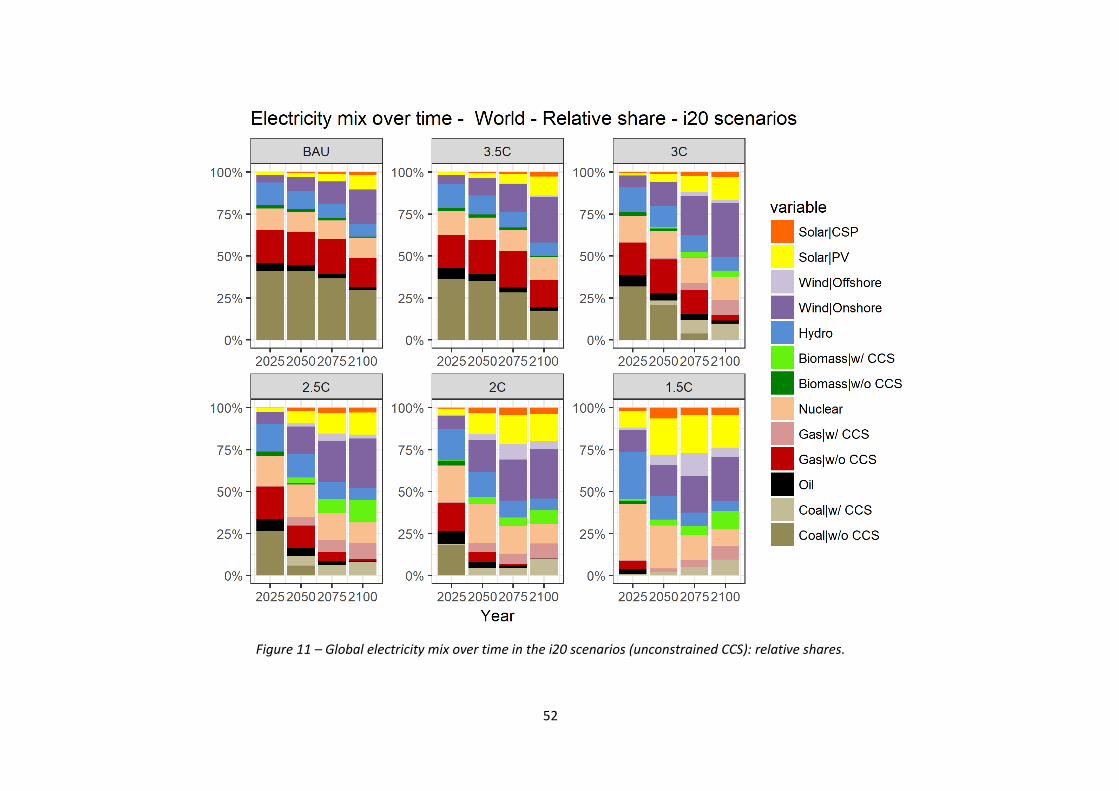
Figure 11 – Global electricity mix over time in the i20 scenarios (unconstrained CCS): relative shares.

53

Figure 12 – Global electricity mix over time in the ioff scenarios (no CCS): absolute generation.

54

Figure 13 – Global electricity mix over time in the ioff scenarios (no CCS): relative shares.

55

Figure 14 shows the policy costs in the different scenarios. Policy costs are evaluated as the cumulated GDP

loss over the century with respect to the cumulated GDP in the baseline case, considering a discount factor

of 2.5%. Values are shown on the same scale, in order to facilitate a comparison of the orders of magnitude

across the different scenarios.

Figure 14 – Policy costs.

Policy costs in the 3.5°C scenarios are negligible, around 0.2%: after all, the stringency of the target is very

mild, so the required changes to the economic and energy systems are almost null. As discussed in the

previous pages, CCS is not deployed in these scenarios, so results are not differentiated per CCS

deployment year within this target. A moderate difference emerges in the 3°C scenarios, where policy costs

are around 0.7-1%. In particular the ioff scenario has a policy cost which is 35% higher than the i20. In the

2.5°C scenarios, policy costs range between 1.9% and 2.7%, with the no CCS case costing 38% more than

the unconstrained CCS scenarios. If reaching 2.5°C entails relatively moderate costs, achieving the Paris-

compatible 2°C target implies much higher expenses. If CCS can be deployed with no constraints, the

aggregated GDP loss is 4.7%. This values increases with a progressively delayed CCS deployment, up to 7.1%

in the no CCS case, 51% more than the former. Finally, the profound revolution which is required to achieve

the 1.5°C target has inevitable enormous effects on the policy costs. With a fully unconstrained technology

portfolio the policy cost is about 16.1%, while it rises up to 27.6% in the corresponding ioff case, i.e. 72%

more than the unconstrained case. Therefore, not only is the delayed deployment of CCS impacting on the

policy cost, but this impact increases in relative terms with the policy stringency.

56

Finally, a brief focus on the European prospects is reported. Indeed, Europe does not have a considerable

storage potential, additionally it is characterized by a huge renewable potential and technology maturity.

These two factors imply that CCS will not be a main mitigation option in this region according to the WITCH

scenarios.

Figure 15 reports the CCS shares in the electricity mix in 2100 in the explored scenarios. As noted in

Figure 7 discussing the global results, CCS does not penetrate the market in the BAU and the 3.5°C

scenarios. Some CCS generation appears in the 3°C scenarios, with a good distribution across the three

considered technologies. Differently from the global results, however, there is no variability as a function of

the CCS deployment year: CCS penetration is around 2-3% independently of when CCS installation is

allowed. This insensitivity to the installation year is found in the more stringent policy scenarios as well,

where, furthermore, CCS penetration i) does not increase significantly with mitigation stringency, and ii) is

almost completely deriving from biomass.

The negligible role played by CCS in the European electricity mix is evident in Figure 16, which shows the

whole electricity mix in the explored scenarios. Already in the BAU case, renewables dominate the long-

term mix, achieving some 70% (about 40% wind and 20% solar, mostly PV, and 10% hydro), which is added

to about 20% of nuclear. Coal and gas sum up to 10% only. Naturally the fossil contribution decreases in the

3.5°C and disappears in the more stringent scenarios, only partially substituted by CCS, as noted, whereas

the remaining technologies essentially maintain their very same shares across all scenarios.

Figure 15 – European CCS relative penetration in the electricity mix in 2100 by source.

57

Figure 16 – European electricity mix in 2100: relative shares

58

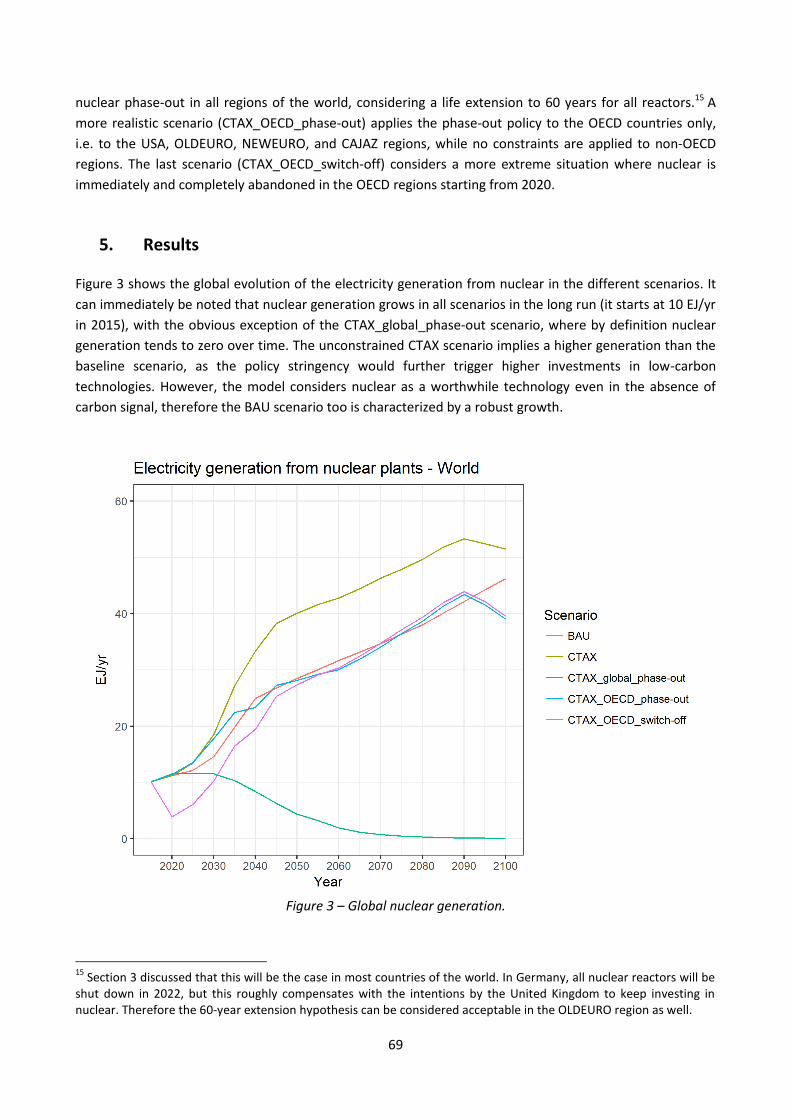
5. Conclusions

CCS is considered one of the key technologies in the perspective of climate change mitigation. Its main

advantage consists in eliminating carbon dioxide emissions without shifting away from the fossil-based

paradigm which still characterizes the power sector. However, in reality many issues still hinder its

diffusion, such as safety concerns about storage sites, public acceptance, high technology costs, and the

absence of a common regulatory framework and of business models.

The main aim of this work is to explore the techno-economic consequences that a delayed deployment of

CCS can have on the electricity mix and on the economic system as a whole. Five deployment options have

been considered with reference to the starting year from which CCS installation is allowed: 2020 (i.e. the

unconstrained scenario, as global CCS capacity is practically negligible as of today), 2040, 2060, and 2080, in

addition to the no CCS scenario. These five scenarios have been explored over a wide set of policy targets,

ranging from the no policy or Business-as-Usual, which leads to 4°C as a temperature increase in 2100 with

respect to the pre-industrial levels, to 1.5°C.

Scenarios confirm the consolidated result in the literature that CCS is likely to play a major role in the

decarbonization of the electricity sector at a global level, as it is installed in all scenarios with a policy target

equal to 3°C or less. In all these cases, as soon as the investment in CCS is allowed, this option is

immediately activated by the optimization model. Due to expansion constraints, the delayed installation

prevents CCS from reaching the optimal level which would be achieved in the unconstrained scenarios.

This implies a progressively lower penetration in the electricity mix as the deployment is delayed: global

CCS penetration is around 25-30% in 2100 in all scenarios from 1.5°C to 3°C, gradually decreasing to zero as

the deployment is delayed or not allowed. The contribution from coal, gas, and biomass is quite well

balanced. The impact on the overall electricity demand is such that it diminishes with the progressively

delayed CCS deployment. This decrease is indeed quite little if mitigation is limited to 2°C (the difference is

lower than 5% in 2100 from the no CCS to the unconstrained CCS scenario), while it is more marked in the

1.5°C scenarios, where the difference in 2100 between the two extreme investment cases (i.e. i20 and ioff)

is around 15%. The absence of CCS is mostly compensated by renewables (notably wind and solar), with

also a partial increase in nuclear.

Removing (partially or totally) CCS from the optimal electricity mix has inevitable effects on the overall

economic performance. The analysis on the changes in policy costs has shown that, within the specific

policy targets, the no CCS scenario is characterized by a cumulative GDP loss which is averagely 50% higher

than the corresponding unconstrained CCS scenarios, thus proving the strong economic impact of the

delayed CCS deployment.

Special attention has also been put on Europe. Indeed, this region is characterized by low availability of

storage sites for CCS and by high renewable potential and technology maturity. This results in a very low

CCS penetration in all scenarios: even in unconstrained conditions and in the most stringent scenarios, CCS

never exceeds 5% in the electricity mix in 2100. The obstacles to CCS penetration are thus much more

relevant on a global level as a whole than specifically on a European level.

59

References

Bosetti V., Carraro C., Galeotti M., Massetti E., and Tavoni M. (2006), WITCH: A World Induced Technical

Change Hybrid Model, Energy Journal, Special issue on Hybrid Modeling of Energy-Environment Policies:

Reconciling Bottom-up and Top-down, 13-38

Bosetti, V. and Longden, T. (2013). Light duty vehicle transportation and global climate policy: The

importance of electric drive vehicles, Energy Policy, Vol. 58, pp. 209-219

Carrara S. and Longden T. (2017). Freight futures: The potential impact of road freight on climate policy,

Technological Forecasting and Social Change, Vol. 55, pp. 359-372

Carrara S. and Marangoni G. (2017), Including system integration of Variable Renewable Energies in a

Constant Elasticity of Substitution framework: the case of the WITCH model, Energy Economics, Vol. 64,

pp. 612-626

Creutzig, F., E. Corbera, S. Bolwig, and C. Hunsberger (2013). Integrating place-specific livelihood and

equity outcomes into global assessments of bioenergy deployment, Environmental Research Letters, Vol. 8,

035047

Davidson, C. L., R. T. Dahowski, H. C. McJeon, L. E. Clarke, G. C. Iyer, and M. Muratori (2017). The Value

of CCS under Current Policy Scenarios: NDCs and Beyond, Energy Procedia, Vol. 114, pp. 7521-7527

Emmerling J., Drouet L., Reis L.A., Bevione M., Berger L., Bosetti V., Carrara S., De Cian E., D'Aertrycke

G.D.M., Longden T., Malpede M., Marangoni G., Sferra F., Tavoni M., Witajewski-Baltvilks J., and Havlik P.

(2016), The WITCH 2016 Model - Documentation and Implementation of the Shared Socioeconomic

Pathways, FEEM Working Paper 2016.042

GCCSI, Global CCS Institute (2017). Global status of CCS: 2017

Havlík, P., Valin, H., Herrero, M., Obersteiner, M., Schmid, E., Rufino, M.C., Mosnier, A., Thornton, P.K.,

Böttcher, H., Conant, R.T., Frank, S. Fritz, S. Fuss, S., Kraxner, F., and Notenbaert A. (2014). Climate change

mitigation through livestock system transitions, Proceedings of the National Academy of Sciences (PNAS),

Vol. 111, pp. 3709-3714

IEA, International Energy Agency (2013). Technology Roadmap, Carbon capture and storage

IEA, International Energy Agency (2017). World Energy Outlook 2017

IPCC, Intergovernmental Panel on Climate Change (2005). IPCC special report on carbon dioxide capture

and storage, prepared by Workin Group III of the IPCC

IPCC, Intergovernmental Panel on Climate Change (2014). Climate Change 2014: Synthesis Report,

Contribution of Working Groups I, II, and III to the Fifth Assessment Report of the IPCC

Koelbl, B. S., van den Broek, M.A., Faaij, A.P.C. and van Vuuren, D.P. (2014). Uncertainty in carbon

capture and storage (CCS) deployment projections: a cross-model comparison exercise, Climatic Change,

Vol. 123, pp. 461-476

Krey, V., Luderer, G., Clarke, L., Kriegler, E. (2014). Getting from here to there – energy technology

transformation pathways in the EMF27 scenarios, Climatic Change, Vol. 123, pp. 369-382

60

Muratori, M., Calvin, K., Wise, M., Kyle, P., and Edmonds J. (2016). Global economic consequences of

deploying bioenergy with carbon capture and storage (BECCS). Environmental Research Letters, Vol. 11,

095004

Pietzcker, R.C., Ueckerdt, F., Carrara, S., de Boer, H.S., Després, J., Fujimori, S., Johnson, N., Kitous, A.,

Scholz, Y., Sullivan, P., Luderer, G. (2017). System integration of wind and solar power in integrated

assessment models: a cross-model evaluation of new approaches, Energy Economics, Vol. 64, pp. 583-599

Rogelj, J., Luderer, G., R. C. Pietzcker, E. Kriegler, M. Schaeffer, V. Krey, and K. Riahi (2015). Energy

system transformations for limiting end-of-century warming to below 1.5°C, Nature Climate Change, Vol. 5,

pp. 519-527.

Schellnhuber, H. J., Rahmstof, R. Winkelmann, R. (2016) Why the right climate target was agreed in

Paris. Nature Climate Change, Vol. 6, pp. 649-653.

UNFCCC, United Nations Framework Convention on Climate Change (2015), Paris Agreement

61

Reactor ageing and phase-out policies: global and European prospects for

nuclear power generation

Samuel Carrara1,2*

1 Fondazione Eni Enrico Mattei (FEEM), Milan, Italy 2 Renewable and Appropriate Energy Laboratory (RAEL), University of California, Berkeley, USA

DRAFT COPY – DO NOT CITE

Abstract

Nuclear is considered as a valuable option for the decarbonization of the power generation, as it is a

no-carbon, yet commercially consolidated technology. However, its real prospects are uncertain: if some

countries, especially in the non-OECD area, have been extensively investing in nuclear, many OECD

countries, which host the vast majority of operational reactors worldwide, feature old fleets which will not

be replaced, as phase-out policies are being implemented.

Research scenarios often consider polarized conditions based on either a global unconstrained nuclear

development or a generalized phase-out. The main aim of this work is instead to explore the techno-

economic implications of policy-relevant scenarios, designed on the actual nuclear prospects in the world

regions, i.e. mainly differentiating policy constraints between the OECD and the non-OECD regions.

The analysis, conducted via the Integrated Assessment Model WITCH, shows that nuclear generation

constantly grows over the century, even if in general the nuclear share in the electricity mix does not

significantly change over time, both at a global and at a European level (apart from a temporary increase in

the first part of the century). Over time, and especially if constraints are applied to nuclear deployment, the

nuclear contribution is compensated by renewables (mainly wind and solar PV) and, to a lower extent, by

CCS (only marginally in the EU).

The policy costs related to the nuclear phase-out are not particularly high (0.4% additional global GDP loss

with respect to the unconstrained policy scenario), as they are almost completely compensated by

innovation and technology benefits in renewables and energy efficiency. Phase-out policies applied only to

the OECD regions do not entail any additional policy costs, while non-OECD regions marginally benefit from

lower uranium prices. A sudden shutdown of nuclear reactors in the OECD regions results in a doubling of

these losses and gains.

Keywords: nuclear, power generation, climate change mitigation, Integrated Assessment Models

____________________________

* Dr. Samuel Carrara, Researcher and Marie Skłodowska-Curie Fellow, Fondazione Eni Enrico Mattei (FEEM), Corso Magenta 63, 20123 Milan, Italy. Tel: +39-02-52036932, Fax: +39-02-52036946, E-mail: samuel.carrara@feem.it. This project has received funding from the European Union's Horizon 2020 research and innovation programme under the Marie Sklodowska-Curie grant agreement No 706330 (MERCURY).

62

1. Introduction

Meeting with increasing energy demand via low-carbon solutions is a major goal for the 21st century in

order to avoid detrimental effects on climate (IPCC, 2014). In 2015, almost all world countries signed the

Paris Agreement committing to limiting to 2°C the global temperature increase in 2100 with respect to the

pre-industrial levels and to pursuing efforts to reach 1.5°C, in order to further contain potential negative

impacts (Schellnhuber et al., 2016). Clearly, these targets are very ambitious, since they entail profound

technological and economical efforts as well as political coordination among countries.

Nuclear is widely recognized as one of the main technologies which will play an important role in

decarbonizing the power sector (Krey et al., 2014 and Koelbl et al., 2014). Its main advantage is the

possibility to couple technological maturity (nuclear has commercially been exploited since the 50s of the

20th century) with virtually no carbon dioxide emissions and without the dispatchability issues that affect

variables renewable energies such as wind and solar.1

Nuclear power was characterized by a huge development especially in 70s and 80s. The accidents in Three

Miles Island, USA (1979) and, above all, in Chernobyl, Former Soviet Union (1986) determined a substantial

fall in the investments, mostly due to the safety concerns that were raised by those events. A general

renaissance took place during the first decade of the 21st century, but the accident at the Fukushima-

Daiichi, Japan (2011) revived public concerns about safety, which ultimately resulted in a reconsideration of

the nuclear expansion policies in many countries of the world (Wittneben, 2012). Concerns about nuclear

proliferation, waste management that is still an open issue, the shortage of qualified workforce in the

reactor construction and high or uncertain costs (at least in some areas of the world) are the other main

points representing an obstacle to nuclear diffusion (Ahearne, 2011). The long construction time

(8-10 years) and operational life of plants (40+ years) make the uncertainty concerning electricity demand

and public acceptance particularly relevant in discouraging investments (Cardin et al., 2017).

These factors jeopardize the future prospects of nuclear energy. As will be discussed in Section 3, in general

two opposite tendencies are found worldwide, which roughly distinguish OECD and non-OECD countries. In

OECD countries (with the main exception of the Republic of Korea), on the one hand many nuclear reactors

are approaching the end of their operational life and on the other hand political, social, and economic

constraints hinder the construction of new plants. Therefore, even in presence of massive investments to

extend the operational lifetime of reactors (from about 40 to about 60 years), the prospects in these

countries are controversial. Instead, in non-OECD countries, and especially China, India, and Russia, nuclear

is characterized by high momentum and ambitious expansion plans are in place for the next decades.

In this context, the main objective of this work is to investigate the actual prospects of nuclear and their

consequent impacts on the electricity mix and the policy costs, taking into consideration real-world aspects

such as the policies implemented by countries and the ageing of reactors. This allows exploring more

credible and meaningful scenarios, whereas assessment exercises often consider “digital” options only, i.e.

either a global unconstrained nuclear expansion or global phase-out (Rogner and Riahi, 2013 and

Hof et al., 2019). The exercise is carried out with the Integrated Assessment Model (IAM) WITCH.

1 It is true, though, that the functioning and huge dimensions of reactors (averagely around 1000 MW, up to 1600 MW

in the latest models) result in a general inflexibility, so that a plant normally operates at full rate 7-8000 hours per year with limited load variations. These aspects could be addressed by developing smaller plants, the so-called Small Modular Reactors (SMRs), whose commercial maturity, however, is yet to come (Budnitz et al., 2018).

63

The paper is structured as follows. Section 2 describes the WITCH model, and especially how nuclear is

modeled therein. Section 3 discusses more in detail the nuclear global scenario and the policy context, and

in particular the policies implemented or planned by world countries. Section 4 describes the scenario

design which has been defined according to the policy landscape described in the previous section.

Section 5 presents the main results of the analysis. Section 6 finally concludes.

2. Methodology

2.1 The WITCH model2

The tool adopted in this research is the World Induced Technical Change Hybrid (WITCH) model. WITCH is a

dynamic optimization Integrated Assessment Model designed to investigate the socio-economic impacts of

climate change over the 21st century (Bosetti et al., 2006 and Emmerling et al., 2016). It combines a top-

down, simplified representation of the global economy with a bottom-up, detailed description of the

energy sector, nested in a Constant Elasticity of Substitution (CES) structure (Figure 1). The model is defined

on a global scale: countries are grouped into thirteen aggregated regions, which strategically interact

according to a non-cooperative Nash game. The thirteen economic regions are USA (United States),

OLDEURO (Western EU and EFTA countries3), NEWEURO (Eastern EU countries), KOSAU (South Korea,

South Africa, and Australia), CAJAZ (Canada, Japan, and New Zealand), TE (Transition Economies, namely

Russia and Former Soviet Union states, and the non-EU Eastern European countries), MENA (Middle East

and North Africa), SSA (Sub-Saharan Africa except South Africa), SASIA (South Asian countries except India),

EASIA (South-East Asian countries), CHINA (People’s Democratic Republic of China and Taiwan), LACA

(Latin America and Central America) and INDIA (India).4 As the model acronym suggests, technological

change is endogenously modeled in WITCH, and it regards energy efficiency and the capital cost of specific

clean technologies. Global prices of fossil fuels are endogenously calculated, while the model is coupled

with the Global Biosphere Management Model, GLOBIOM (Havlík et al., 2014) to describe land use.

GLOBIOM provides biomass supply cost curves to WITCH for different economic and mitigation trajectories.

This allows assessing woody biomass availability and cost.

The CES structure reported in Figure 1 shows how the top-down aggregated economic model is linked with

the disaggregated energy sector. In particular, energy services (ES) and the aggregated capital and labor

node (KL) are combined to produce the final economic output of the model. Energy services are provided

by the combination of the capital of energy R&D (RDEN), which is a proxy of energy efficiency, and the

actual energy generation (EN). This node models the fact that the same energy services can be obtained

through a lower level of energy input if there is higher energy efficiency. The EN node is divided between

the electric (EL) and non-electric sector (NEL), with a progressive disaggregation down to the single

technologies. The electric sector has a higher detail, while the non-electric sector mostly reports nodes

which collect consumption from all the non-electric usages of one specific energy source, except for the

road passenger and road freight transport sectors, which are the only demand sectors being explicitly

modeled5 (see Bosetti and Longden, 2013, and Carrara and Longden, 2017).

2 For the sake of simplicity, this section has almost entirely been taken from the CCS paper.

3 EFTA (European Free Trade Association) features Iceland, Liechtenstein, Norway, and Switzerland.

4 The aggregated results for Europe derive from the combination of OLDEURO and NEWEURO.

5 These sectors are not shown in the CES scheme.

64

Figure 1 – The CES structure in WITCH.

Focusing on the electric sector, the hydroelectric technology is found first (ELHYDRO), which is essentially

exogenous in the model. The other technologies converge to the EL2 node, which is divided between two

further nodes: EFLFFREN, i.e. the combination of fossils and renewables, and ELNUKE&BACK, i.e. the

combination of nuclear and backstop. The fossil node (ELFF) has three group of technologies:

i) coal&biomass (ELCOALBIO), further divided into pulverized coal without CCS (ELPC), pulverized biomass

without CCS (ELPB), integrated gasification coal with CCS (ELCIGCC), and integrated gasification biomass

with CCS (ELBIGCC); ii) oil, only without CCS (ELOIL); iii) gas (ELGAS), with and without CCS (ELGASTR and

ELGASCCS, respectively). Variable renewable energies (ELW&S) have i) wind (ELWIND), further divided

between onshore (WINDON) and offshore (WINDOFF); ii) solar PV (ELPV); iii) solar CSP (ELCSP). Nuclear and

backstop feature traditional fission nuclear (ELNUKE) and a backstop technology (ELBACK). The latter

models a hypothetical future technology which generates electricity with no fuel costs and no carbon

emissions, although characterized by high capital costs. It can be interpreted as an advanced nuclear

technology, for instance nuclear fusion or advanced fast breeder fission reactors. However, this technology

is not considered in the scenarios explored in this work. Concerning the non-electric sector, the first

distinction is between traditional biomass (TradBiom), coal (COALnel) and the aggregated node formed by

oil, gas, and modern biomass (OGB), which precisely features gas (GASnel), traditional biofuels (Trad Bio),

and the combination (OIL&BACK) between oil (OILnel) and a non-electric backstop technology, i.e.

advanced biofuels (BACKnel).

The CES structure tries to capture from a modeling point of view the preference for heterogeneity that is

experienced in the real world, where the choice of investing in energy technologies does not normally

depend on economic considerations only. The numbers reported in the CES scheme under the specific

65

nodes indicate the relevant elasticity of substitution. As suggested by the name, this value quantifies the

level of substitutability between the sub-nodes that converge to the specific node. Zero elasticity means

that the production factors are not substitutable and thus they are summed in fixed shares. Infinite

elasticity means that the production factors are completely interchangeable and thus the competition

between the two occurs on an economic basis only. Intermediate elasticities result in an intermediate

behavior. More details concerning the CES structure can be found in Carrara and Marangoni, 2017.

2.2 Nuclear modeling

The investment cost for new nuclear plants is 4709 $/kW6. The same cost is applied to all world regions,

even if in reality some differences may be found. Future model improvement will differentiate costs across

regions. O&M costs do vary across regions, instead. Only fixed O&M costs are explicitly considered, which

are comprised between 160 $/kW and 220 $/kW, while no variable O&M are accounted for. However,

waste management and storage costs are explicitly considered: they start at 0.1 c$/kWh in 2015 and

increase slightly more than linearly with the relative increase in nuclear generation (MIT, 2003), which is a

direct proxy of waste production. Uranium ore is considered sufficiently abundant to meet the increasing

nuclear demand over the century, and in particular reserves are considered sufficiently large at prices

below 350 $/kg, i.e. the level at which reprocessing spent fuel and fast breeder reactors become

competitive, which would prevent any further rise in the uranium price (Bunn, 2005). The process of

conversion, enrichment, and fuel fabrication of the uranium ore is also taken into account, and the relevant

cost is fixed to 300 $/kg (MIT, 2003). The efficiency of nuclear power plants is 35%, the capacity factor is

85%, while the standard lifetime is 40 years (Tavoni and van der Zwaan, 2011).

3. Nuclear global landscape

As of November 30, 2018, there are 454 operational reactors in 31 countries worldwide, with an equivalent

net capacity of 400 GW, while 54 reactors are under construction in 18 countries (4 of which not included

in the previous 31), with an equivalent net capacity of 55 GW (IAEA, 2018).7,8 Additional 26 countries have

decided or have been considering to invest in nuclear, even if no reactors are practically under construction

yet (Budnitz et al., 2018). Figure 2 shows the global situation in terms of operational and under

construction rectors, also specifying the age of the former, grouping countries according to the WITCH

regions. In the following, a brief description of the current status and the implemented policies is provided

for each region.

The USA have 98 operational reactors, i.e. the highest number worldwide. The American fleet is also the

oldest, as the average reactor age is around 38 years, i.e. close to the reference operational life of 40 years.

On the other hand, only two reactors are under construction, expected to come online in 2021 and 2022

respectively (Gattie et al., 2018). This means that the US are going to face severe ageing issues in the

coming decades. Indeed, as mentioned in the Introduction, the operational lifetime of a nuclear reactor can

normally be extended from 40 to 60 years, if dedicated upgrade and revamping works are carried out

6 Costs are expressed in USD2015.

7 These figures indicate that the average capacity for each reactor is about 1 GW. This will implicitly be assumed in the

following: capacity will explicitly be specified only if different from this reference value. 8 Henceforth, the reference IAEA, 2018 will implicitly be assumed for all statistical data if not differently specified.

66

(Perrier, 2018). This strategy is extensively applied in the US (Volk et al., 2019), and most reactors have

already obtained the relevant authorization (Davis, 2012). Still, in the absence of investment in new

reactors, the retirement of the existing ones will begin around 2030 and will result in a complete phase out

in some 20 years (Gattie et al., 2018).

Figure 2 – Regional distribution of nuclear reactors and their age.

Similar conditions occur in the OLDEURO region, i.e. in Western Europe. Here the operational reactors are

112 with an average age of 35 years, whereas only two reactors are under construction, specifically in

France (Flamanville) and Finland (Olkiluoto). Construction works for additional two reactors will shortly be

started in the United Kingdom (Hinkley Point). All these four plants are EPR (European Pressurized

Reactors) of 1.6 GW of net capacity each. With its 58 reactors, France is the country which relies most on

nuclear: this technology accounted for about 71% of the total national electricity generation in 2017. The

plan would be to decrease this share to 50% in 2025, but this target is unlikely to be met (Volk et al., 2019).

Most likely, life extension programs will be implemented. In 2010, Germany had 17 operational reactors

and approved a policy allowing the extension of the reactors operational lifetime by averagely 12 years.

The Fukushima accident in 2011 determined a radical change: the oldest 8 reactors were immediately shut

down, while the remaining 9 will be closed within 2022, well before their planned operational end

(Rogner, 2013). Most of the other countries have been implementing similar yet milder phase-out policies,

as early retirement is not normally considered and life extensions are often planned or applied. These

countries are Sweden (8 reactors), Belgium (7), Spain (7), Switzerland (5), and the Netherlands (1), which

will all phase out within the next twenty years. The same applies to Finland apart from the plant under

construction in Olkiluoto (its four operational plants are already about 40 years old). The United Kingdom

plans to phase out its 15 plants (accounting for 9 GW) within 2030, but, apart essentially from France, it is

the only country in the region considering nuclear as the main carbon mitigation technology, so that 16 GW

67

of new installations are planned in the next years (Volk et a., 2019). All in all, a strong capacity reduction is

easily forecastable in this region in the near future.

A similar situation is found in NEWEURO, i.e. Eastern Europe, which features 19 operational reactors, with

an average age of almost 30 years, and two reactors under construction (in Slovakia). Lithuania, Bulgaria

and Slovakia had partly to shut down their old plants as one of the conditions to be admitted to the EU

(Volk et a., 2019). The remaining plants will progressively be phased out in the next decades.

The CAJAZ region includes the country that obviously has most been affected by the Fukushima accident,

i.e. Japan. Nowadays, 42 of the 54 existing plants in 2011 are still considered operational (while two are

under construction), even if only 5 have generated electricity in 2017, whereas the remaining 37 are still

waiting for decisions on their future (Volk et al., 2019). However, the Japanese government still aims at

achieving a nuclear share in the electricity mix of 20-22% in 2030 (WNA, 2018a), i.e. slightly below the pre-

Fukushima levels, as the share was equal to 26% in 2010 (IEA, 2012). Canada essentially replicates the

conditions of the other Western countries: old reactors, no new constructions ongoing, and investment in

extending the operational life.9

The KOSAU region is quite peculiar within the OECD regions. The core country here is the Republic of

Korea. This country has 24 relatively recent reactors (the average age is 21 years) and it has strongly been

investing in nuclear: 5 reactors are under construction and plans are to continue along this path in the next

decades, which makes the Republic of Korea the only Western country strongly investing in nuclear without

major issues. South Africa has two operational reactors which are 33 and 34 years old, respectively. Plans

to build new capacity within 2030 have been suspended, therefore only life extension interventions may

reasonably be considered in this country for the near future (WNA, 2018b).

Transition Economies (TE) face similar problems as Western countries in terms of ageing of nuclear

reactors, as most reactors were built during the Cold War in the 70s and 80s and are currently undergoing

works for life extension (Volk et al., 2019). However, considerable investments in new capacity are in place,

especially in Russia (6 reactors are under construction), but also in Ukraine (2), Belarus (2), and Turkey (1),

which allows forecasting optimistic futures for nuclear in this region.

Middle East and North Africa (MENA) is a “young” nuclear region. The first plant was inaugurated in the

Islamic Republic of Iran in 2011, while 4 reactors are under construction in the United Arab Emirates, with

works expected to progressively end in the very next years. No other countries have implemented or

planned investments, however.

Sub-Saharan Africa except South Africa (SSA) and South-East Asian countries (EASIA) do not have any

operational nor under construction reactors.10

South Asian countries (SASIA) have considerably been investing in nuclear. Pakistan has a very recent fleet,

as 3 of its 5 reactors were inaugurated in the last decade, and two additional reactors are under

construction. Two reactors are also under construction in Bangladesh.

The same applies to the main other South Asian country, that is an independent region in WITCH, i.e.

INDIA. 22 operational reactors with an average age of 23 years and 7 reactors under construction highlight

bright prospects for nuclear in this country.

9 Nuclear power plants are not present in New Zealand, and no different plans are in place. The same will apply to

Australia in the KOSAU region. 10

For an overview on the nuclear debate in the EASIA countries, see Putra, 2017.

68

A similar and even more positive scenario is found in CHINA: its 46 reactors have an average age of 7 years

and 11 plants are under construction. Similarly to India, huge development can be predicted for the next

decades, as nuclear is considered an excellent technology to cope with the enormous growth in energy

demand while also meeting with the climate mitigation requirements. For this region, it should be noted

that Taiwan is a nuclear country: here prospects are less bright, as the four operational reactors are

approaching the age of 40 and the construction of two reactors has recently been suspended.11 It is clear,

however, that the dimensions of this country are not such as to affect the overall evaluation of the CHINA

region.

Finally, Latin and Central America (LACA) features three countries with nuclear power plants, i.e. Argentina,

Brazil, and Mexico. There are 7 operational reactors in the region, with quite a high average age (28 years).

Two reactors are under construction, and plans (especially in Argentina, see WNA, 2018c) are to continue

investing in this technology. Hence, the nuclear share in this region is not very high, but it is expected to at

least maintain its levels in the coming future.

To conclude, this overview has described in detail the general distinction between the OECD and non-OECD

regions (with the exception of the Republic of Korea)12 that had been anticipated in the Introduction:

optimistic nuclear prospects can be expected for most non-OECD countries that have nuclear power, and

especially Russia, India, and China, while more complicated futures can be estimated for OECD countries.

4. Scenario design

The nuclear landscape described in the previous section is the main reference for the definition of the

scenarios explored in this exercise. Indeed, the coherent picture which characterizes the OECD and the

non-OECD countries allows considering a limited set of scenarios, which are five in total.

First of all, a baseline or Business-as-Usual (BAU) scenario has been run as a benchmark. No mitigation

policies nor other technological constraints are considered in this scenario.

The other four scenarios are explored in a mitigation policy compatible with the Paris targets. In particular,

a uniform carbon tax is applied in all regions starting from 2020 so as to reach a global cumulative amount

of CO2 emissions equal to 1000 Gt in the period 2011-2100. This would limit the temperature increase in

2100 with respect to the pre-industrial levels below 2°C with a likely chance (IPCC, 2014). In particular, this

corresponds to a temperature increase of 1.8°C in WITCH, whereas the baseline scenario leads to a

temperature increase of about 4°C. In terms of annual global CO2 emissions, the policy scenarios entail a

constant decrease from 36 Gt/yr in 2015 down to -8 Gt/yr in 210013, while the no policy scenario has CO2

emissions constantly growing to about 75 Gt/yr until around 2080, then remaining substantially constant

until the end of the century.14

One scenario (CTAX) is run without any other constraints, and in particular nuclear energy is freely

optimized by the model in all regions. On the opposite, one scenario (CTAX_global_phase-out) considers a

11

These two reactors formally still appear as under construction in IAEA, 2018, however. 12

The exception of the Republic of Korea among the OECD countries will implicitly be assumed henceforth with no further specification. OECD regions in this work will thus be USA, OLDEURO, NEWEURO, and CAJAZ. 13

Negative emissions can be reached via biomass CCS and afforestation in WITCH. 14

The overall greenhouse gas emissions (GHG) start at 50 GtCO2eq/yr and increase to 93 GtCO2eq/yr in 2100 in the baseline scenario, while they decrease to -3 GtCO2eq/yr in the policy scenarios.

69

nuclear phase-out in all regions of the world, considering a life extension to 60 years for all reactors.15 A

more realistic scenario (CTAX_OECD_phase-out) applies the phase-out policy to the OECD countries only,

i.e. to the USA, OLDEURO, NEWEURO, and CAJAZ regions, while no constraints are applied to non-OECD

regions. The last scenario (CTAX_OECD_switch-off) considers a more extreme situation where nuclear is

immediately and completely abandoned in the OECD regions starting from 2020.

5. Results

Figure 3 shows the global evolution of the electricity generation from nuclear in the different scenarios. It

can immediately be noted that nuclear generation grows in all scenarios in the long run (it starts at 10 EJ/yr

in 2015), with the obvious exception of the CTAX_global_phase-out scenario, where by definition nuclear

generation tends to zero over time. The unconstrained CTAX scenario implies a higher generation than the

baseline scenario, as the policy stringency would further trigger higher investments in low-carbon

technologies. However, the model considers nuclear as a worthwhile technology even in the absence of

carbon signal, therefore the BAU scenario too is characterized by a robust growth.

Figure 3 – Global nuclear generation.

15

Section 3 discussed that this will be the case in most countries of the world. In Germany, all nuclear reactors will be shut down in 2022, but this roughly compensates with the intentions by the United Kingdom to keep investing in nuclear. Therefore the 60-year extension hypothesis can be considered acceptable in the OLDEURO region as well.

70

The constraints on nuclear growth in the OECD countries are such that nuclear generation is significantly

lower in the CTAX_OECD_phase-out and the CTAX_OECD_switch-off scenarios than in the unconstrained

CTAX scenario, essentially replicating the BAU results. In the CTAX_OECD_switch-off, in particular, nuclear

generation starts to grow immediately after the 2020 shock, implying that the growth in the non-OECD

countries more than compensates the generation end in the OECD countries. Indeed, the lower uranium

demand in the OECD countries related to these scenarios implies lower fuel prices for non-OECD countries.

This boosts nuclear generation considerably higher than in the CTAX scenario, see Figure 4.

Figure 4 – Nuclear generation in non-OECD regions.

The global electricity demand does not markedly change among the four policy scenarios, even if there is a

considerable difference between them and the BAU scenario, see Figure 5. This graph also indirectly

highlights an important aspect of decarbonization. In general decarbonization can be achieved via two main

strategies. The first one is to reduce emissions simply by reducing energy demand. This is the most

straightforward strategy, as it does not entail a profound reconfiguration of the energy sector, and is what

happens in the policy scenarios in the short term: here the electricity demand grows very mildly, compared

to a more consistent growth in the BAU scenario. However, whereas the increase in the BAU scenario is

fairly regular over the century, in the policy scenarios the electricity demand starts growing very fast after

about 2040 and it overcomes the BAU levels around 2070/2080. This happens because the second

decarbonization strategy is now deployed, which consists in increasing the share of electricity in the overall

secondary energy demand with a parallel decarbonization of the electricity sector (which in general

guarantees the easiest decarbonization routes).

71

Figure 5 – Global electricity demand across scenarios.

Figure 6 – Global nuclear share across scenarios.

72

The evolution of the nuclear share in the electricity generation mix (Figure 6) naturally derives from the

combination of Figure 3 and Figure 5. The 2015 level of 11% is more or less constant over the century in the

BAU scenario, as the nuclear growth is substantially in line with the overall electricity demand growth

(around 2% per year). The CTAX_global_phase-out is obviously characterized by a constant decrease to

zero, while all the other policy scenarios show a marked increase until about 2040 (to a maximum level

which is progressively lower as the stringency of the constraints on nuclear increases, i.e. 25% in the CTAX

scenario, 19% in the CTAX_OECD_phase-out scenario, 16% in the CTAX_OECD_switch-off scenario), which is

followed by a decrease down to the initial levels towards the end of the century.

This happens because of the tremendous growth of renewables, notably wind and solar PV, which

progressively gain market shares and become dominant in the second part of the century. This fact is

clearly visible in Figure 7 and Figure 8, which show the evolution of the electricity mix at a global level in

four selected years (2025, 2050, 2075, and 2100): the former shows the absolute generation, while the

latter shows the relative shares.

First of all, both figures highlight that the carbon tax applied in the policy cases is such that the electricity

sector is already fully decarbonized by 2050, when only a residual share of gas without CCS still appears in

the electricity mix. This obviously does not apply to the BAU scenario, where fossils do not suffer from any

constraints and they still maintain almost half of the generation portfolio in 2100, despite a growth in

renewables which progressively become attractive even in the absence of the carbon tax.

The behavior of electricity demand has already been discussed above: in 2025 and 2050 this is higher in the

BAU scenario than in the policy ones, in 2075 the levels are similar, while in 2100 the policy scenarios show

a much higher demand. Here it is interesting to note an additional point: it has been said that the overall

demand is similar across the policy scenarios, but a more precise observation would highlight that it grows

with respect to the unconstrained CTAX scenario if constraints (phase-out or switch-off) are applied to the

OECD countries, and even more if phase-out regards all regions. This happens because the constraints on

nuclear imply higher investments in the other low-carbon technologies. Since WITCH features an

endogenous technological modeling of the investment cost for renewables – in particular, wind onshore,

wind offshore, solar PV, and solar CSP, while this does not apply to hydro and CCS – this implies

considerable innovation benefits for wind and solar technologies, that are thus able to reach higher

generation levels, which more than compensates the reduction or the absence of nuclear generation. As a

result, the aggregated penetration of solar and wind technologies reaches 35% of the electricity mix in

2100 in the BAU scenario, 54% in the CTAX scenario, 59% in the CTAX_OECD_phase-out as well as the

CTAX_OECD_switch-off scenarios, and 67% in the CTAX_global_phase-out scenario.

The sever impact that such a considerable penetration of variable renewable energies would have on the

energy system is a topical and well-known issue. The stability of electrical grid requires that demand and

supply be constantly in balance and this is not trivial if generation comes from plants fueled with a variable

energy source. Abstracting from the technical aspects, it is not easy to model this issue in Integrated

Assessment Models: these phenomena take place on very small spatial and temporal scales, whereas IAMs

generate scenarios which span an horizon of decades, providing average annual quantities and considering

large, aggregated regions. It is not within the scope of this paper to thoroughly discuss such an aspect. To

this purpose, the reader is referred to Carrara and Marangoni, 2017 for further details on the WITCH model

and to Pietzcker et al., 2017 for an overview of IAMs. However, one effect, i.e. the deployment of huge

storage capacity to sustain the renewable expansion, can be easily highlighted: see Figure 9 which shows

the power capacity evolution in the same selected years as Figure 7 and Figure 8.

73

Figure 7 – Global electricity mix over time: absolute generation.

74

Figure 8 – Global electricity mix over time: relative generation shares.

75

Figure 9 – Global electricity mix over time: capacity.

76

It can be noted that, whereas considerable storage capacity is required in the second half of the century (in

addition to a similar growth in the electric infrastructure, not shown here), this is not necessary in the first

half, when the moderate renewable growth can be “absorbed” by the remaining generation fleet which

provides sufficient flexibility.

Moving the attention on the regional results, Figure 10 shows the evolution of the nuclear share in the

unconstrained CTAX scenario in the thirteen WITCH regions (as well as at global level for comparison

purposes).

Figure 10 – Regional nuclear share in the CTAX scenario.

The graph shows that, for most regions, the optimization model provides results in line with the actual

policy landscape and prospects. Nuclear generation remains zero or close to zero in the regions which

today have neither reactors nor investments plans, i.e. EASIA and SSA, and in the regions which do have a

small nuclear share but do not have any particular expansion plans, i.e. LACA and MENA. The nuclear share

instead grows in the regions which have ambitious expansion plans: CHINA, INDIA, KOSAU, SASIA, and TE,

at least until mid-century. After that date, as already discussed, nuclear does not stop growing in absolute

terms, but it does so slower than renewables, which gain more and more market shares, so that the

relative nuclear shares decreases. On the other hand, the nuclear share immediately starts decreasing in

those regions which are characterized by critical nuclear prospects, such as CAJAZ and OLDEURO, where

decarbonization is mostly carried out via renewables and, for the former, CCS. The only two regions not

fully in line with the actual policy landscape are NEWEURO and USA, which show a marked growth despite

the present conditions which do not suggest such an evolution for the next decades.

77

Remaining at a regional level, it is interesting to focus on the European results. Europe is naturally given by

the combination of OLDEURO and NEWEURO, where the former substantially accounts for 90% of the total

in terms of economic and social weight between the two.

First of all, Figure 11 shows the evolution of the nuclear share in Europe. The main aim is naturally to

compare the BAU and the CTAX scenarios, which essentially have the same progress, with a substantial

constancy of the nuclear share over time. The CTAX_global_phase-out, CTAX_OECD_phase-out, and

CTAX_OECD_switch-off scenarios, in fact, show a trivial behavior. In the latter, nuclear generation

immediately falls to zero in 2020, while in the two phase-out scenarios (which are equivalent for Europe),

the share gradually decreases to zero over the next decades.

Figure 11 – European nuclear share across scenarios.

Figures 12, 13, and 14 show the generation (in absolute and relative values) and the capacity mixes in the

four selected years for the five scenarios. Two major differences emerge from the global results. First, the

renewable penetration is considerable already in the BAU scenario, where fossils have a marginal role even

in the absence of a climate policy. Therefore it is not surprising that these technologies dominate (with

nuclear) the power landscape in the mitigation scenarios. Second – and related to the first – the CCS

penetration is negligible: this is due to the low availability of storage sites and, again, to the high potential

and technology maturity that renewables have in this region. The enormous penetration of solar and wind

is such that a corresponding amount of storage capacity is needed to ensure grid stability, as clearly shown

in Figure 14.

78

Figure 12 – European electricity mix over time: absolute generation.

79

Figure 13 – European electricity mix over time: relative generation shares.

80

Figure 14 – European electricity mix over time: capacity.

81

It is finally interesting to assess the economic impacts of the different scenarios, and in particular the policy

costs. These costs are evaluated as the cumulated GDP loss over the century with respect to the cumulated

GDP of the baseline case, considering a yearly discount factor of 2.5%. First of all, Figure 15 shows the

policy costs in the different regions in the unconstrained CTAX scenario, which is the benchmark of the

mitigation scenarios portfolio.

Figure 15 – Regional policy costs in the CTAX scenario.

The average global GDP loss is 8.3%. However, marked differences are found across regions. MENA and TE

are the two regions which by far are affected most by the mitigation policies: the GDP loss amounts to

about 23% here. This result is unsurprising, as these are the two main exporters of fossil fuels: the

implementation of the carbon tax results in a global drop of fossil consumption and so happens to the

economic performance of these regions, which is added to the lower domestic consumption that the policy

allows. On the other end, OLDEURO is the region which is affected least by the mitigation policy: GDP loss is

less than 3% here. Also in this case no major surprise can arise: the previous figures have shown that in this

region a considerable decarbonization already takes place in the BAU scenario, i.e. the economic

optimization per se leads to a low-carbon portfolio without the implementation of a carbon policy, which

simply expands this tendency.

Focusing on the economic impacts of the nuclear phase-out or switch-off policies, a previous paper (De

Cian et al., 2011) explored this aspect highlighting a point that has already been mentioned in the previous

pages: the innovation benefits regarding the technologies which undergo learning (signally wind and solar),

82

as well as the overall efficiency of the energy sector, result in lower costs (investment costs for renewables

and for the energy sector in general) which essentially compensate the phase-out costs. But what happens

at regional level? And what are the impacts of differentiated policies? Figure 16 shows the policy costs in

the remaining three mitigation scenarios, highlighting the difference with respect to the unconstrained

CTAX scenario in percentage points. This is done in order to abstract from the effects of the mitigation

policy, and focus on the pure effects of the nuclear policy.

Figure 16 – Regional policy costs in the mitigation scenarios: difference with respect to the CTAX scenario.

The TE result immediately emerges in the CTAX_global_phase-out scenario: the additional GDP loss is 5.3%,

markedly more than any other region in all the considered scenarios. Considering that the GDP loss in the

CTAX scenario is already equal to 23%, this means an overall loss of 28%. The reason must be found in

Figure 10: TE is the region that would invest more in nuclear, and the innovation benefits related to

renewables are completely insufficient to compensate the absence of a technology that, in the

unconstrained CTAX scenario, would almost reach 60% of the generation share towards mid-century. All

the other regions are not extraordinarily affected by the global phase-out (the additional losses are within

1%). The specific results, however, depend on the nuclear penetration that would be achieved in the

unconstrained scenario, therefore it is not surprising that SASIA, CHINA, INDIA, and NEWEURO show the

highest additional losses and that the three regions where nuclear would not be deployed anyway, i.e.

EASIA, MENA, and SSA, even gain (although quite marginally) from the global phase-out. MENA, in

particular, can benefit from the slightly higher gas demand, to be used in CCS plants. The global additional

GDP loss is less than 0.4%, again highlighting the almost total compensation of the policy cost via the

-5.3%

83

innovation benefits. To put this number in perspective, an equivalent scenario with a constraint applied to

CCS instead of nuclear would entail a 5%-growth in the policy cost (Carrara, this issue), which is even more

remarkable considering the lower average share over the century that CCS would achieve in the

unconstrained policy scenarios with respect to nuclear.

If the phase-out is limited to the OECD regions (CTAX_OECD_phase-out), a clear polarization is found. The

OECD regions show the economic loss of renouncing nuclear, even if being the only regions which phase

out does not cause any additional costs with respect to the global phase-out scenario (i.e. the additional

GDP loss in the OECD regions is practically the same in the central and in the left-hand graphs). The non-

OECD regions show very marginal benefits (apart from TE, for the reasons described above), essentially

related to the lower costs of uranium deriving from the OECD phase-out.

Finally, the CTAX_OECD_switch-off shows the same qualitative behavior as the CTAX_OECD_phase-out

scenario, even if results are quantitatively more marked, given the higher stringency of the technological

constraint. The OECD regions show an additional GDP loss which is averagely around 1%, while the relative

gain in the non-OECD regions is averagely 0.2% (almost 1% in TE), i.e. losses and gains approximately

double.

6. Conclusions

Nuclear is expected to be one of the key technologies in the future power landscape, especially if

mitigation policies are implemented. Its main advantage consists in generating electricity with a

consolidated and well-known technology without emitting carbon dioxide. However, many issues, and

especially public acceptance, hinder its deployment in many areas of the world. This is added to concerns

about nuclear proliferation and waste management, the shortage of qualified workforce in the reactor

construction and high or uncertain costs.

The nuclear landscape is very polarized between OECD and non-OECD countries. The former feature the

most numerous fleets, but most reactors are approaching the end of their operational life and

governmental policies are in most cases against further nuclear development and only consider dedicated

investments for the lifetime extension of existing reactors. The latter instead, apart from some regions

which do not feature and do not intend to invest in nuclear, show higher momentum and more ambitious

expansion plans, especially China, India, and Russia.

This work has explored the techno-economic implications of policy-relevant nuclear scenarios, designed on

the actual prospects for this technology in the world regions, i.e. mainly differentiating policy constraints

between OECD and non-OECD regions.

Results show that global nuclear generation is expected to grow in all unconstrained scenarios (BAU and

CTAX), with a higher growth in the policy case, as in this scenario nuclear partly compensates the

retirement of fossil plants. If constraints (phase-out and switch-off) are applied to nuclear in the OECD

regions, nuclear growth is more moderate, and is in line with the BAU scenario. Naturally, in the

CTAX_global_phase-out, nuclear generation globally tends to zero over few decades. The considerable

growth in terms of generation does not correspond to an analogous marked growth in terms of share in the

electricity mix, as the overall electricity demand grows accordingly. Indeed, in the policy scenarios the share

does significantly increase in the first decades, but then it approximately returns to the 2015 levels, in

correspondence of the huge expansion of renewables (notably wind and solar PV) which prevail on nuclear

84

and CCS in the mitigation portfolio. The huge expansion of variable renewable energies entails the

deployment of a substantial storage capacity, which is needed to ensure grid stability.

The electricity landscape is not very different in Europe. However, this region is characterized by low

availability of CO2 storage sites and by high renewable potential and technology maturity, which hinder the

penetration of CCS technologies. Therefore, power generation is dominated by wind and solar without

major alternatives.

The implementation of a mitigation policy has well-known negative economic effects (the cumulated global

GDP loss over the century is about 8% with respect to the baseline scenario), especially in the fossil

exporting countries (23% GDP loss in MENA and TE), as the need for decarbonization implies a strong

reduction in fossil consumption. The additional policy costs related to the nuclear constraints, however, are

not substantial, as most regions have an additional GDP loss of less than 0.5% (0.4% at a global level): this

happens because the phase-out costs are almost completely compensated by the innovation benefits in

the renewable and the overall energy efficiency areas stimulated by the nuclear phase-out itself. TE shows

an additional 5%-loss, being the region that would have the highest nuclear penetration in the

unconstrained scenarios. If constraints are applied to the OECD regions only, no additional losses are found

here with respect to the global phase-out scenario, while the non-OECD regions slightly benefit from the

lower uranium costs. The CTAX_OECD_switch-off scenario simply exacerbates these results: the average

additional GDP loss in the OECD regions and the average GDP gain in the non-OECD regions approximately

double.

References

Ahearne, J.F. (2011). Prospects for nuclear energy, Energy Economics, Vol. 33, pp.572-580

Bosetti, V., Carraro C., Galeotti M., Massetti E., and Tavoni M. (2006), WITCH: A World Induced Technical

Change Hybrid Model, Energy Journal, Special issue on Hybrid Modeling of Energy-Environment Policies:

Reconciling Bottom-up and Top-down, 13-38

Bosetti, V. and Longden, T. (2013). Light duty vehicle transportation and global climate policy: The

importance of electric drive vehicles, Energy Policy, Vol. 58, pp. 209-219

Budnitz, R.J., Rogner, H.H., and Shihab-Eldin, A. (2018), Expansion of nuclear power technology to new

countries – SMRs, safety culture issues, and the need for an improved international safety regime, Energy

Policy, Vol. 119, pp. 535-544

Bunn, M., Fetter, S., Holdren, J.P., and van der Zwaan (2005). The economics of reprocessing versus

direct disposal of spent nuclear fuel, Nuclear Technology, Vol. 150, pp. 209-230

Cardin, M.A., Zhang, S., and Nuttall, W.J. (2017). Strategic real option and flexibility analysis for nuclear

power plants considering uncertainty in electricity demand and public acceptance, Energy Economics,

Vol. 64, pp. 226-237

Carrara S. (this issue). The techno-economic effects of the delayed deployment of CCS technologies on

climate change mitigation

Carrara S. and Longden T. (2017). Freight futures: The potential impact of road freight on climate policy,

Technological Forecasting and Social Change, Vol. 55, pp. 359-372

85

Carrara S. and Marangoni G. (2017), Including system integration of Variable Renewable Energies in a

Constant Elasticity of Substitution framework: the case of the WITCH model, Energy Economics, Vol. 64,

pp. 612-626

Davis, L.W. (2012). Prospects for nuclear power, Journal of Economic Perspective, Vol. 26, pp. 49-66

De Cian, E., Carrara, S., and Tavoni, M. (2014). Innovation benefits from nuclear phase-out: Can they

compensate the costs?, Climatic Change, Vol. 123, N. 3-4, pp. 637-650

Emmerling, J., Drouet L., Reis L.A., Bevione M., Berger L., Bosetti V., Carrara S., De Cian E., D'Aertrycke

G.D.M., Longden T., Malpede M., Marangoni G., Sferra F., Tavoni M., Witajewski-Baltvilks J., and Havlik P.

(2016), The WITCH 2016 Model - Documentation and Implementation of the Shared Socioeconomic

Pathways, FEEM Working Paper 2016.042

Gattie, D.K., Darnell, J.L., and Massey, J.N.K. (2018). The role of U.S. nuclear power in the 21st century,

The Electricity Journal, Vol. 31, pp. 1-5

Havlík, P., Valin, H., Herrero, M., Obersteiner, M., Schmid, E., Rufino, M.C., Mosnier, A., Thornton, P.K.,

Böttcher, H., Conant, R.T., Frank, S. Fritz, S. Fuss, S., Kraxner, F., and Notenbaert A. (2014). Climate change

mitigation through livestock system transitions, Proceedings of the National Academy of Sciences (PNAS),

Vol. 111, pp. 3709-3714

Hof, A.F., Carrara, S., De Cian, E., Oehler, P., Pfluger, B., van Sluisveld, M.A.E., and van Vuuren, D.P.

(2019). From global to national scenarios: bridging different models to explore power generation

decarbonisation based on insights from socio-technical transition case studies, forthcoming on

Technological Forecasting and Social Change

IAEA, International Atomic Energy Agency (2018). PRIS, Power Reactor Information System,

https://pris.iaea.org/PRIS/home.aspx

IEA, International Energy Agency (2012). World Energy Outlook 2012

IPCC, Intergovernmental Panel on Climate Change (2014). Climate Change 2014: Synthesis Report,

Contribution of Working Groups I, II, and III to the Fifth Assessment Report of the IPCC

Koelbl, B. S., van den Broek, M.A., Faaij, A.P.C. and van Vuuren, D.P. (2014). Uncertainty in carbon

capture and storage (CCS) deployment projections: a cross-model comparison exercise, Climatic Change,

Vol. 123, pp. 461-476

Krey, V., Luderer, G., Clarke, L., and Kriegler, E. (2014). Getting from here to there – energy technology

transformation pathways in the EMF27 scenarios, Climatic Change, Vol. 123, pp. 369-382

MIT, Massachusetts Institute of Technology (2003). The future of nuclear power: an interdisciplinary MIT

study

Perrier, Q. (2018). The second French nuclear bet, Energy Economics, Vol. 74, pp. 858-877

Pietzcker, R.C., Ueckerdt, F., Carrara, S., de Boer, H.S., Després, J., Fujimori, S., Johnson, N., Kitous, A.,

Scholz, Y., Sullivan, P., and Luderer, G. (2017). System integration of wind and solar power in integrated

assessment models: a cross-model evaluation of new approaches, Energy Economics, Vol. 64, pp. 583-599

Putra, N.A. (2017). The dynamics of nuclear energy among ASEAN member states, Energy Procedia,

Vol. 143, pp. 585-590

86

Rogner, H.H. (2013). World outlook for nuclear power, Energy Strategy Reviews, Vol. 1, pp. 291-295

Rogner, M. and Riahi, K. (2013). Future nuclear perspectives based on MESSAGE integrated assessment

modeling, Energy Strategy Reviews, Vol. 1, pp. 223-232

Schellnhuber, H. J., Rahmstof, R., and Winkelmann, R. (2016) Why the right climate target was agreed in

Paris. Nature Climate Change, Vol. 6, pp. 649-653

Tavoni, M. and van der Zwaan, B. (2011). Nuclear versus coal plus CCS: a comparison of two competitive

base-load climate control options, Environmental Modeling & Assessment, Vol. 16, pp. 431-440

Volk, R., Hübner, F., Hünlich, T., and Schultmann, F. (2019). The future of nuclear decommissioning – A

worldwide market potential study, Energy Policy, Vol. 124, pp. 226-261

Wittneben, B.B.F. (2012).The impact of the Fukushima nuclear accident on European energy policy,

Environmental Science & Policy, Vol. 15, pp. 1-3

WNA, World Nuclear Association (2018a). Nuclear Power in Japan, http://www.world-nuclear.org,

retrieved on November 30, 2018

WNA, World Nuclear Association (2018b). Nuclear Power in South Africa, http://www.world-

nuclear.org, retrieved on November 30, 2018

WNA, World Nuclear Association (2018c). Nuclear Power in Argentina, http://www.world-nuclear.org,

retrieved on November 30, 2018