Delivery4D: an open–source model–based Bayesian seismic inversion program for time-lapse problems James Gunning [email protected]CSIRO ESRE, 71 Normanby Road, Clayton North Victoria, 3169, Australia, ph. +61 3 9545 8396 July 5, 2013 Abstract An extension of the open–source Bayesian AVO inversion program Delivery [1],[2] to time–lapse seismic inversion problems is described. The inverse problem is for a trace–wise layer–stack model comprising unknown layer–times, rock properties, fluid types and saturations, and pore pressure changes. The “data” are true–amplitude imaged/migrated seismic reflectivity traces, for arbitrary numbers of stack angles and vintages. Both maximum aposteriori models and posterior samples, via MCMC, are made available. Coupling to stress is made via local calibrated regression models, and saturation via Gassmann’s relations. Test problems demonstrate upper limits on what might be reasonably inferred about saturation from seismic data alone, and show distinct refinement in “swept” zones, but small improvements elsewhere. 1
An extension of the open–source Bayesian AVO inversion program Delivery [1],[2]to time–lapse seismic inversion problems is described. The inverse problem is for atrace–wise layer–stack model comprising unknown layer–times, rock properties, fluidtypes and saturations, and pore pressure changes. The “data” are true–amplitudeimaged/migrated seismic reflectivity traces, for arbitrary numbers of stack angles andvintages. Both maximum aposteriori models and posterior samples, via MCMC, aremade available. Coupling to stress is made via local calibrated regression models,and saturation via Gassmann’s relations. Test problems demonstrate upper limits onwhat might be reasonably inferred about saturation from seismic data alone, and showdistinct refinement in “swept” zones, but small improvements elsewhere.
Time–lapse seismic monitoring of oil and gas reservoirs has now become a routine procedurein the oil and gas industry. Despite the many challenges involved in acquiring reproduciblesurveys and processing heterogeneous surveys to a mutually comparable basis, many suc-cessful applications of time–lapse or 4D seismic for reservoir planning or monitoring useshave been claimed [3].
There are many critical steps involved in obtaining useful 4D data. The acquisition andprocessing steps must be designed carefully to maximise reproducibility and suppress noise.Signals from changing reservoir conditions can be quite weak, so it is important that thesenot be overwhelmed by surface noise or acquisitional footprints of various kinds. At present,it is still usual to process data sets independently, though a deal of the processing will useshared earth models, such as the kinematic framework velocities. The imaging model–spaceof the short scale reflectivity is usually computed independently, so an opportunity to jointlyconstrain these imaged reflectivities from expected vintage–continuity of short–scale featuresis missed in these conventional workflows.
In the near–reservoir region, more detailed, rock–physics based inversions operating onthese imaged reflectivities have an opportunity to enforce these vintage–continuity consid-erations. Reflectivities arise from rock–property contrasts, and such contrasts will vary onlyif deterministic fluid and stress movements affect the bounding rock properties. Clearly,if multi–vintage seismic data is to be adequately “explained” by some common, evolvingshared earth model (or an ensemble of models), suitable physical models of the evolvingprocesses controlling stress and saturations are necessary. Thus, we may expect that inver-sion of seismic data for an earth modelling comprising elastic and petrophysical propertiesevolving forward in time can only be guaranteed to be physically consistent if it comprisescoupled flow simulation, rock physics, geomechanics, and wave propagation. Such an rigor-ous inversion –especially with measures of uncertainty – is beyond current technical capacity.But there are limits of these models where some of the processes are not important, or atleast approximately representable using simpler models than computer–intensive 3D partialdifferential equations. Commonly, for example, stress effects are less important, or less com-plex, in fields which are larger and have high fluid mobilities. Similarly, in gravitationallydominated recoveries, the evolving saturation profiles are simpler and more piston–like. Ibelieve there are a modest range of field conditions in which inversion of an earth modelbased on imaged seismic data with naive models for fluid movement and stress behaviourcan be useful.
Since time–lapse data is shot only on fields of commercial value that are well into de-velopment, it is nearly always the case that the main formation units comprising the fieldare well studied, mapped, and characteristic elastic properties of the salient rock types areavailable from log data. Such “formation–scale” models are usually layer–based, and builtat scales that are seismically resolvable. This geometric sequence of layers and its forwardevolution in time with fluid movement and stress is a natural basis for a model to invert fromtime–lapse seismic data. The formations themselves are often well modelled by fine–scalespatial mixtures of a small group of rock–types, for example, laminated or dispersed clay insandstone. A particular seismic trace of imaged reflectivity is consistent with this model if aforward synthetic model computed from the model “matches” the observed trace in a suit-able sense. With appropriate models to project the rock properties and geometric structure
3
forward in time, the “matching” criterion stated above can be imposed simultaneously onlater vintage seismic traces in the same location.
At any particular transverse spatial location, a suitable mathematical structure for theseformation sequences with imperfectly known times/depths and layer properties is a jointmarked–point model for kinematics/geometry, and a parametric model for rock–properties.The stochastic geometry is represented by time parameters for layer tops, and the stochas-tic properties by layer–based rock mixtures with mixing parameters such as net–to–grossfor permeable–rock fraction, and end–member rock types whose elastic properties are char-acterised by Bayesian prior distributions estimated from log data. The notion of “tracematching” above can be expressed more formally as a Bayesian likelihood, which will becouched in terms of matching the full reflectivity image waveform, not just arrival times.
For single–vintage seismic data, such a model–based Bayesian inversion has been imple-mented in the Delivery code, which has evolved over some ten years to acquire a varietyof modelling flexibility [2]. This paper describes the modelling assumptions and conceptualmodels that have been used to extend the Delivery code to time–lapse problems. The chiefingredients are effectively regression based models for capturing stress effects, and simplerock–physics theories for projecting the rock properties forward over the vintage sequenceto model the saturation effects as well. The primary stress variables parasite on globalpredictor trends generated from pore–pressure models, but these are usually available fromproduction reservoir models, and the pressure is usually a fairly smooth, robust quantity.
The notation, context, and assumptions of the standard single–vintage Delivery imple-mentation (see the extended paper at [2]) are presumed known in this paper. For unfamiliarreaders, a potted summary of the model is this: at each common–image point or trace, asequence of layers with time–parametric tops (and a final lower base time) presents reflectioninterfaces to an impinging wavelet at prescribed incident angle for each stack. See Fig. 1.Each layer is a fine–scale laminar mixture of up to 3 rock types; 1 reservoir, and 1 (or 2)non–reservoir, with 1 (or 2) net–to–gross parameters carving up the volume. The reservoirend–member rock type can undergo fluid substitution with several types of hydrocarbon flu-ids, with possibly variable saturation parameters, under the assumption of fine–scale fluidmixing. The effective layer properties are computed by a sequence of effective media calcula-tions for fluid mixing, Gassmann substitution, and rock inter–bedding via Backus averaging,and these effective properties enter suitable AVO relations for the reflection coefficients asa function of angle. Bayesian prior distributions estimated from log data control the al-lowable range of rock elastic properties (vp, vs, ρ) for each contributing facies. These priormodels roughly capture loading and correlation effects. Similar distributions from manualor computer–assisted interpretation establish prior beliefs about where the layers occur intime. Priors beliefs about fluid saturations can be encoded either explicitly using mapsof fluid kinds and saturations, or implicitly modelled by moving fluid contacts specified indepth interacting with the saturation prior. The time models are co–registered in depth byhanging computed thicknesses (velocity×time) on a supplied depth surface attached to areference layer.
I have confined the theory below chiefly to an account of the modelling relations andapproximations describing time–lapse effects. Most of the details of the forward physics,statistical sampling algorithms etc, are the same as described in [2]. The paper follows theusual layout of theory, demonstration synthetic problems, discussion, conclusions. A fieldtest is discussed in a separate paper.
4
oil-filled laminated sand
brine-filled laminated sand
brine-filled laminated sand
shale
shale
shale
oil-filled laminated sand
brine-filled laminated sand
brine-filled laminated sand
shale
shale
shale
oil-filled laminated sand
brine-filled laminated sand
brine-filled laminated sand
shale
shale
shale
tt
Reflection
coefficients
Synthetic
seismic
wavelet
m = {t ,NG, φs , vp,s , vs,s , ρm ,vp,m, vs,m, S h }
Typical model parameters m per layer, some vintage-variable:
s = reservoir rocks
m = impermeable rocks
h = hydrocarbon
Multi-vintage model at trace
V1V2
V3
Picks and geological interpretation Forward model per
stack+vintage
2.10
2.15
2.20
2.25
2.30
10 20 30 40 50
Figure 1: Schematic of how the local layer–based model is assembled, with synthetic seismicdata associated with each vintage and stack at each trace location.
2 Theory
The response of reservoir and near–reservoir rock saturation and stress variables to fieldproduction varies a good deal in complexity, with depositional environment, heterogeneity,fluid mobilities, and operational design as important factors. Flow simulation studies invari-ably show more spatial uniformity and smoothness in pressure and stress than saturation,which follows from the elliptic–like equations that control the elastic response. The rela-tive smoothness of the pore–pressure response is what invites the rough elasticity modelapproximations used below. The code operates on a trace–local layer based model, assum-ing the imaged reflectivity is well approximated by a convolutional model operating on thesequences of reflectivities occurring at each layer interface in time. Since much of the fol-lowing discussion focuses on the additional modelling relations I have added to this model,it is useful to set out some notational conventions early.
Layer numbers are denoted i (i = 1 . . . Nl), facies/rock–types are labelled Fi for facies Fin layer i, T is an index for a seismic vintage, or seismic time–snapshot T = 1, 2 . . . NT (e.g.base–shoot, 1 year monitor, 5 year monitor), and Θj,T an index for (angle–) stack numberj at vintage T . Where I address fluid contacts, kf,T is an index running over all fluid unitsand contact types (see [2] for definitions of fluid units and contact types) at vintage T .
The approximate models described in the following section necessarily involve both quasi–empirical constants and additional parameters to the model, which must be equipped withBayesian prior distributions approximately capturing prior prejudices and uncertainties. Theappearance of any new parameters will be associated with new prior–distribution specifica-tions in the model configuration files.
5
2.1 End–member rock types under stress and saturation changes
Stress
Much of the modelling in this section amounts to crude approximations to more subtlematerial found in Colin Sayers’ SEG DISC course [4]. For simplicity, the elastic variablesin all layers at at trace are modelled as having a smooth, empirically fitted, non–historydependent response to pore–pressure changes in a chosen reference layer (often the mainproduction layer), for the direction and extent of expected stress variations. “Smooth” meansdeterministic over the regime and direction of stress changes experienced by the model andfor which the inverse calculation is expected to be valid.
The overall stress dependence of velocities is undoubtedly nonlinear and path–dependentfor large changes. Empirical data is commonly fitted with nonlinear forms like Bowers’ rela-tion, or exponential curves which saturate beyond characteristic effective stresses. For largechanges, hysteretic effects are important, so the benefit of nonlinear forms is questionable.For example, in Hatchell and Bourne[5], velocity changes are estimated from timing shiftsin key surfaces observed over multiple 3D surveys acquired over a long time span. They fitthe velocity change empirically in terms of measured strain via:
δv/v = Rǫzz
where R is a dimensionless constant. The chief finding of this paper is that the (strain)coefficient R is a factor of 2 or so larger for rocks undergoing extension (usually surroundingshales) compared to the reservoir. Also, the R values for rocks undergoing compression isfairly close to what might be derived from the porosity–velocity regression, assuming thegross character of such a regression was mainly due to the effects of loading. This finding ispossibly good evidence of the hysteretic effect mentioned above.
The important conclusion seems to be that the R coefficients need to be obtained dy-namically (i.e. from triaxial or actual pore–pressure change measurements), and that thesensitivity in elongation is larger than compaction. The chosen empirical constants must beappropriate for the expected direction of loading, and where this direction is not a–priorideterminable, a suitable compromise is probably best.
The way the stress couples to layers other than the reference/production layer is a func-tion of the reservoir geometry, the spatial distribution of geomechanical properties, and isgenerally a computationally intensive 3D geomechanical problem. For certain typical ge-ometries (pancake reservoirs etc), the character of this stress distribution is amenable to“cartoon” representations, wherein the induced stress in all the layers can be decently ap-proximated by a linear correlation with the main (reference layer) pore pressure change.The correlation coefficients are analytical available for simple models like ellipsoids.
The elasticity relations in this inversion model are of this simple class. Though simplis-tic, the model has the merit that the stress–path coefficients can be customized on a facies,base–stress, and path dependent basis. A nonlinear form could equally well be used if theoverall fractional velocity changes are large, but this would likely entail additional empir-ical constants. Such linearisations are also obtainable from various commonly used fittingrelations for velocity dependence, e.g. Bowers’ relation.
End–member rock properties are modelled by
vp,F,i,T ≡ vp,F,i,1 + Reffp,F,T Ui,iref
∆pT (1)
6
where ∆pT is the pore–pressure change (relative to T = 1) in the reference layer iref, Reffp,F,T
is an effective stress path coefficient apposite for the production scenario, the rock type andthe time, and Ui,iref
is the cross–correlation coefficient from stress between the referencelayer and the layer i. The stress–path coefficients may be obtained by e.g. the gradientof suitable tri–axial core–test velocity data versus pore–pressure for each rock type, for thecorrect directions of stress change at in-situ conditions. The pore–pressure and stress–pathcoefficients can be in any consistent set of units with velocity. Elastic modelling or a cartoonanalytical model will supply the correlation coefficients Ui,iref
. A complex version could usespatially varying U ′s. At this stage, the coefficients are globally static constants.
In the existing Delivery model, end–member rock properties are equipped with priordistributions which roughly capture within–facies property correlations, loading, and dis-persion. Thus, for example, the base–vintage prior distributions for vp and vs are factoredas
where depth–rock–curves and LFIV are prior–model supplied predictor values (maps) forloading effects, Ap, Bp, Cp, As, Bs regression constants, σvp,s regression errors, and latervintage (end–member) velocities differ from this value only via the coupled effects from ∆pT .Analogous relations for the shear–velocity, the porosity, and density apply. At present, therelations used are
vs,F,i,T = vs,F,i,1 + Bs,FReffp,F,T Ui,iref
∆pT T > 1 (4)
φF,i,T = φF,i,1 T > 1 (5)
which corresponds to shifting shear velocity along the normal loading curve with the p–wave velocity (BvF
being the slope of that curve supplied by the regression relations), andneglecting shifts in porosity (since the latter will contribute only via Gassmann). If desired,the obvious extended constitutive model would require a suite of stress–path coefficientsR[p,s,φ,ρ],F,T , to be obtained by laboratory measurements. The coefficients above are correctat loose “leading order”, and since the contributions from vs and volumetric effects from φare small at modest angles, this modelling accuracy is probably about the same as a numberof other factors I have completely neglected.
Saturation
Depending on the nature of the production, mobility ratios, capillarity, formation hetero-geneity, basin hydrology, and a host of other variables, the mobile–fluid spatial distributioncan vary tremendously. Engineers usually think of a triangle of endpoints corresponding togravity, capillary, or viscous/dynamic dominated flows. Complex vertical flows are relativelylikely near wells (coning instabilities), and generally phase boundaries will be more geomet-rically complex as flow rates increase. Some of this may well create scattering or other lossmechanisms for impinging waves.
One cannot hope to be able to capture complex effects like this in a post–imaging inver-sion code, especially when the effects are likely sub–wavelength. The current implementation
7
continues the simple models of using Gassmann–style substitution for the effect of pore–fluidchanges on bulk end–member elastic character. Some kind of approximate regression modelto approximate patchy or fingering saturation effects is conceivable, but not used in thecurrent approach. The existing implementation thus implies fluids are well–mixed at thepore–scale either throughout a layer, or within the relevant contacts in depth. Clearly thesaturation variables are then some kind of induced “effective–saturation” construct.
2.2 Fluids
Delivery has two styles of handling fluid variation, enumeration, and fluid contacts. Themanner in which these styles can be applied to time lapse problems is rather different, andtreated separately below.
Enumeration
In this case, layers are fully “inhabited” by a particular fluid type, conveniently chosen from{b,l,o,g}= {brine, low–sat gas (lsg), oil, gas}. Nontrivial prior probabilities for each fluidtype in each permeable layer, together with a user–specified density ordering style, are usedto assemble a list of discrete allowable fluid modes with associated overall prior probabilityFor example, a 3 layer model with 6 fluid configuration possibilities may be
g g o g o bg o o b b bb b b b b b.
With multiple T vintages a simple and reasonable model is to insist the “fluid–case” remainconstant for a particular forward model and that the saturation variables then track themovement of fluids. The saturation priors can be made vintage (T ) dependent.
I have coded functionality to optionally enforce modelling constraints like monotonicityin the T–sequence of saturations (say, a depletion production schedule), both in the optimi-sation and sampling phases. For example, if the new saturation variables are Sf,T,i (f=o,gsince lsg is immobile), we might like to enforce the ordering Sf,Tj+1,i ≤ Sf,Tj ,i. This isimposed through additional rejection steps in the sampler, and polytope–bound constraintsin the optimiser. One simple and reasonable model is to write the saturation prior for latervintages as a “Tobit” model where the saturation is truncated at one end by the saturationof the previous vintage, analogous to the existing way we truncate the Normal prior fornet–to–gross at 0 or 1 with the Gaussian tail collapsed onto the end of the [0, 1] interval.Mathematically, this gives the prior for the suite of saturations of a particular hydrocarbontype in the ith layer as
P ({Sf,Tj ,i}) =
Nv∏
j=1
N(Sf,Tj ,i, σSf,Tj,i),
but the actual saturations S′ used in any likelihoods (i.e. forward physics) are given by thesequential projections
if, for example, the relation Sf,Tj+1,i ≤ Sf,Tj ,i is chosen. The piling up of prior probabilityonto surfaces of matching saturation is a reasonable characteristic, as this approximatelycaptures a mixture component one would like to have in the prior model corresponding to“no change”. An example might be totally unswept areas, where we’d expect saturations tomatch at subsequent vintages.
At present, for oil or gas saturations, the code offers users the facility of setting theattributes vintage (an integer) and ordering ∈ {none, less than, equals, greater than}. Thisforces the saturation to satisfy the chosen relation in comparison to the saturation of theprevious vintage, for the same layer at the current trace, in the sense of the truncation modeljust described.
Fluid contacts
The original aim of the fluid–contacts model was to impose flatness of contacts (in depth)for pre–production models as an additional constraint when the models have modest depthuncertainty. If the nature of the production is likely to create a modestly sharp movingcontact at each time-snapshot (usually fairly permeable systems with little heterogeneity,strong fluid density contrasts, benign mobility ratio, and probably primary production),one could approximately model the moving interface using contacts with tight saturationuncertainties. In this case the machinery will impose only one “fluid case”, and contactvariables will be added to the modelling vector. One of the examples later on illustrates thismode of modelling.
With the contacts model, one may want to supplement the prior with a fluid–contactstemporal ordering requirement, e.g. that the contacts rise monotonically with the vintageindex. For unproduced areas, it is desirable to be able to accumulate probability for theconfiguration where the contacts do not move, so again a Tobit–like truncation model isuseful. Thus the depth variables for each contact are both allowed to “vary areally”, but canalso be equipped with the attribute ordering ∈ {none, less than, equals, greater than}, whichspecifies a relational ordering to the corresponding contact depth at the previous vintage. Theimplied Tobit–like mappings to true contact depths Z ′ are thus, for a particular fluid contact
Z ′
Tj= min(ZTj−1
, ZTj) j = 2 . . . Nv,
if we specify less than for all contact–depths associated with this contact (e.g. a GB contact),i.e. require ZTj+1
≤ ZTj.
2.3 Times and Depths
Under production and significant stress, the time and depth of all layers can potentiallychange. The effect of travel–time changes in the gross overburden is outside the scope ofthe Delivery model, but I have tried to capture the effect at the price of an additional∆τT mis–registration variable, per vintage, attached to the reference layer. All other layertimes are registered from the mutual consistency of thicknesses, velocities, and times. Thus,
9
extrapolating from existing Delivery notation, we have;
tiref,T = tiref,1 + ∆τT T > 1 (6)
ti,T = tiref,T +∑
i > iref : j = iref . . . i − 1i < iref : j = i . . . iref − 1
2∆zj,T
vp,eff,j,T(7)
The shift variable ∆τT will be equipped with a Gaussian prior ∆τT ∼ N(∆̄τT , σ2∆τT
). Settingσ∆τT
= 0 will naturally remove the parameter from the stochastic model.The basic approach I take for reconstruction of the later vintage time/depth geometries
is preservation of thicknesses, and this default model is the only one implemented at present.A conceivable issue in rather unusual (perhaps deep, overpressured) reservoirs is construct-ing a model for later thicknesses ∆zj,T where the stresses are so great that appreciablestrain deformation occurs. In cases where the actual thickness changes are significant, thesestrains are probably of a non-reversible destructive kind, so experimental measurement ofthe relevant in–situ elastic constants is doubtless challenging.
The following is a sketch of the theory that might be used where deformations are impor-tant. Taking ∆zi,1 ≡ (ti+1,1 − ti,1)vp,eff,i,1/2 as the base–case thickness, subsequent thick-nesses are treated as a pseudo–compliance–driven perturbation from this, cross–correlatedfrom the strain induced in the reference layer: ∆zi,T = ∆zi,1 + SiUi,iref
∆pT . Later–vintagetimes could be set from these deformed thicknesses. The pseudo–compliances Si must beuser supplied from geomechanical models. If the strain is more than a fraction of a per-cent the pseudo–compliance constant very likely includes irreversible deformation, and themodel is only “linear” in a directed (i.e. irreversible) sense. The limit Si = 0 correspondsto preservation of thicknesses, and this is likely a sensible default for most situations wherethe rock response is modestly reversible. Only in unusual situations is the expected strainlikely to be more than a fraction of a percent, so usually this effect can be ignored.
2.4 Likelihoods
The revised code has extended functionality to both an arbitrary number of vintages, an ar-bitrary number of stacks per vintage, and possible use of difference stacks for later vintages.These additional sources of data are treated, somewhat naively, as independent sources ofinformation, each contributing a term to an extended product form of likelihood. Doubt-less there exist correlations both temporally, between stacks, and between vintages, whichdiminish the true information count of the data relative that which accrues under the inde-pendence assumption. A good deal of this correlation is model–induced, and thus systematiceven across multiple vintages. There is thus no simple or objective way of estimating suit-able correlation structures to embed in the likelihood function. A practical suggestion isto use very few stacks (since the AVO relations virtually guarantee significant redundancyover a small angle range), and discount the estimated noise levels from well ties to accountfor modelling systematics. Blind validation tests are doubtless useful at wells. This is adifficult, problematic topic, which I can at best genuflect to at this point.
For mathematical and computational simplicity we write the likelihood function associ-ated with the synthetic seismic mismatch as a standard quadratic likelihood
Here the “unrolled” data vector S = {SΘj,T} is the full set of seismic data for all vintages
T and angles Θj,T concatenated to one long vector, e.g. S = {SΘ1,1,SΘ1,2
,SΘ2,2} for a 2–
vintage survey with near–stack at the earlier time, but nears+fars in the second survey. Thecovariance CD in principle absorbs all the complex correlation effects mentioned above, butis extremely difficult to estimate meaningfully in practice. A diagonal approximation willbe used, with (in perhaps increasing order of questionability), independence between sam-ples, vintages, and angles. The entries are estimated from well tie and wavelet extractionsperformed for each vintage.
can also be added, where the ∆s denote differences from some nominal base survey, e.g.∆S = {SΘ1,2
− SΘ1,1,SΘ2,2
− SΘ2,1}, and the difference error covariance estimated also
from well–ties. The arguments for this kind of term revolve around the subtraction processremoving various systematic contributions to the noise process, and thus yielding a tighterposterior prediction. Difference stacks are likely safer to use in the regime where stress effectsare weak. If they are used, a workable process is to perform well–ties on difference stacks andintroduce these as “pseudo–stacks’ at their requisite vintage with the associated wavelets.This will introduce the required likelihood terms, albeit with an independent noise processfrom the constituent vintages. The current implementation allows for difference stacks tobe used only if the before/after associated stacks are included as well, but this is what mostsensible workflows would do anyway.
2.5 Overall model listing
For completeness, I enumerate here the full possible contributions to the stochastic modelvector from all the features described. The complete model is a union of layer–based pa-rameters and global parameters, the latter being a motley collection of contact–related and“sundry” variables;
m = {mlayer,i,T}i=1...Nl,T=1...NT∪ mglobal (10)
mglobal ≡ mcontacts ∪ msundry. (11)
Extending the Delivery notation again (s=permeable, m=impermeable), for T = 1, the layermodel can in principle include
mlayer,i,1 = {ti, [tbase, i = Nl], drock curves,i,1,LFIVi,1,
In realistic applications a large fraction of these parameters are disabled or inoperative. Typ-ically, e.g. the density of fluids will be assumed known and constant, the rock regression willhave fixed loading depths (drock curves) and LFIV, lithological complexity will be simplifiedetc, yielding a much reduced set of parameters per layer. The parsing and code bookkeepingcan further remove any trivial or non–contributing parameters from the runtime overhead.
2.6 Styles of saturation modelling
The apparatus available at present enables three different kinds of fluid–movement mod-elling. Various blends of these are also possible, but interpretations of the outputs must bemade carefully. In summary, these are
• Fixed fluid–case, variable saturation models. Here, the fluid types occupying a layerare fixed in the model by setting the desired fluid probabilities to unity on a trace-by–trace basis. This allows only one discrete “fluid–state” in the delivery model. Changingsaturations are modelled by setting loose priors on the saturation variables which areexpected to change between vintages. Distinct priors for saturations at each vintageare possible. These sorts of models will often reveal ambiguities between saturationand net–to–gross, especially when the seismic doesn’t change. See example 5.1.
• Moving contact models. Here, the sequence of occupying fluids is prescribed by asuite of fluid contacts specified in depth. Loose and vintage–dependent priors on thesefluid contact depth variables enable the movement of fluids to be modelled. Fixed oruncertain saturations can be introduced on a per–vintage basis. See example 5.2.
• Multi–fluid case models can also be used by specifying fluid probabilities other than0 or 1. together with e.g. loose saturation priors. The posterior distributions inthese models can be expected to be complex mixture distributions, and may not beespecially easy to interpret (e.g. low–saturation oils look like brine etc).
3 Workflows
Setting up and running a time–lapse inversion project using the extended Delivery4D coderequires some substantial preparatory work. For convenience, the main steps are summarisedhere.
• Assemble true–amplitude imaged seismic reflectivity data for all the vintages andstacks of interest. Difference cubes may also be used. invariably these are “cookie-cut”to a study area of interest.
12
• Perform joint wavelet extractions on all quality wells in the area to be inverted, forall vintages. Post–production extractions can be challenging, as “effective” time-lapselog data is difficult to procure.
• Form rock–physics trends for all salient facies, and assemble fluid and grain data.
• Determine characteristic stress responses of rocks for insitu conditions; collect regres-sion constants for prediction models under expected pore pressure movements.
• Estimate stress cross–correlation coefficients of reservoir layers either from rules ofthumb (usually simple analytic models), or a more complex geomechanical model ifcoupling is expected to be strong.
• Collect surface horizon picks of all surfaces for all vintages, including fluid–contacts ifused.
• Assemble spatial maps of expected saturation or pore–pressure trends from knownreservoir data, e.g. paleo–contacts, flow–simulation pressure distributions.
• Assemble spatial maps of prior net–to–gross, fluid–probabilities (if used), isopachs,and related spatially varying model parameters
• Summarise all spatially varying prior information in a suitable model.su file, withcorrect cross references in the XML file. The file must have the same spatial indexingand ordering as the cookie–cut seismic.
Before firing off inversions, a good deal of probing of the prior model is wise as a sanitycheck. Visualisation of the mean–prior and various sample models is useful for all vintagesnapshots and in a good number of views. These can be generated using the -p, -IS, and -IIflags in various combinations. The mean–prior synthetic model should very preferably havemajor seismic loops coinciding closely with the desired interpretation and data. Major signand amplitude “busts” evident in views of the mean prior synthetics are very likely to causeloop–skipping behaviour in the inversion - the usual evidence of significant conflict betweena model and the data.
A short discussion of the post–processing utility DeliveryAnalyser is in order, beforediscussing the demo inversion cases. This gives some idea as to how some of the graphicalrenderings have been produced from the output of the Delivery4D code.
4 Post–processing: extensions to the DeliveryAnalyser
program
The companion deliveryAnalyser4D has also been extended to time–lapse functionality. Thiscode provides capability to analyse the “realisation” files produced by the inversion, provid-ing useful summary statistics, some graphical views of models, synthetic seismic plots etc.Since the number of possible interrogations of the time–lapse inversion output is very large,some useful functionality may well be implemented by various scripts wrapped around somecore eliveryAnalyser4D invocations.
13
The main change in this code is that properties are accessed by the new syntaxPROP,vintage[:stack] where the name of a property is explicitly required. For example,use vp m,2 for the shale velocity in vintage 2, or R pp,1:2 for a reflection coefficient ofvintage 1, stack 2. (Note that R pp denotes the PS reflection coefficient if the stack isspecified as PS data in PP time).The vintage will default to 1 if not specified, so thedeliveryAnalyser4D syntax is identical to usage in existing non–time–lapse studies (forexample, vp m,1 means the same as vp m). With this convention, most of the existingfunctionality has been carried across in the deliveryAnalyser4D code. Some functions of thedeliveryAnalyser4D code may require a “global” vintage specification via -V vintage, so,e.g. we might look at a layer model for vintage 2 via
• Compute the P50 quantile of net-oil, layer 2, vintage 2:% deliveryAnalyser4D -i realisations.su --quantile net-oil,2 2 50
• Stream out ascii non-reservoir v p samples, layer 3, vintage 1:% deliveryAnalyser4D -i realisations.su -p-ascii vp m,1 3
• Stream out ascii 2–column P–impedances of layer–3 and layer–4 , vintage 1, at namedtrace-location:% cat realisations.su | deliveryAnalyser4D --trace-filter ’cdp=2308,ep=1262’
-p-ascii2-gen Z eff,1 Z eff,1 3 4
• Another way, plotted graphically as a scatterplot:% deliveryAnalyser4D -i realisations.su --trace-filter ’cdp=2308,ep=1262’
-p-ascii2-gen Z eff,1 Z eff,1 3 4 -G
• Plot a section through the MAP model at a particular inline. Default vintage displayedis 1. Grayscale=layers:% deliveryAnalyser4D -i realisation.MAP.su --trace-filter ’cdp=2308’ -l -G
• Similar, rendering density at vintage 2:% deliveryAnalyser4D -i realisation.MAP.su --trace-filter ’ep=1262’ -lprop
rho eff -V 2 -G
• Plot a spaghetti plot of the synthetic seismics from the realisation samples, at locationspecified, for times 1.8 < t < 2.2s, at vintage 2, for stack 1, using supplied wavelet.Superpose seismic from seismicV2S1.su at same location:% deliveryAnalyser4D -i realisations.su --trace-filter ’ep=1262,cdp=2308’
-S 1.8 2.2 R pp,2:1 wavelet.su seismicV2S1.su -G
• Same as above, coregistered with layer-model cross–section: add -lNG, for example.
• Plan view maps of properties can be cobbled together in lots of ways. Using SU andthe shell, for example to get a “most–likely” map of NG at vintage 2, layer 5suchart key1=gx key2=gy < seismic.su | b2a n1=1 > XY.txt
-G As per associated flag (eg -l, -p-ascii)-V v (int) Global vintage spec for selected commands-l from -V-lf from -V-lNG from -V-lZ_eff from -V-lprop prop from supplied prop[,vintage]-Sl seismic_filename.su from -V-Slo seismic_filename.su from -V-ldepth from -V-f from -V--time-to-depth from -V--full from -V--full-means from -V--full-stddevs from -V--full-quantile Q from -V-p PROP N from supplied prop,V (will override -V v)-p-ascii PROP N from supplied prop,V (ignores -V)-p-ascii2 PROP1 PROP2 N from supplied prop1,v1 prop2,v2 (ignores -V)-p-ascii2-gen PROP1 PROP2 N1 N2 from supplied prop1,v1 prop2,v2 (ignores -V)-p-ascii-t from -V-p-ascii-prop PROP from supplied prop,V (will override -V v)-p-ascii-full from -V--mean PROP N from supplied prop,V (will override -V v)--stddev PROP N from supplied prop,V (will override -V v)--quantile PROP N from supplied prop,V (will override -V v)--histogram PROP N from supplied prop,V (will override -V v)--fluid-prob F N from -V-s t_0 t_last R_pp[_fc][,v,s] wavelet.su from -V-S t_0 t_last R_pp[_fc][,v,s] wavelet.su seismic.su from -V--filter PROP [=|>|<] value N from supplied prop,V--filter-pad PROP [=|>|<] value N from supplied prop,V--BHPcommand filename Synchronized to any SU outputs generated--make-prior-traces prop1,prop2,... defaults to vintage 1--massage-analyse Incomplete TO-DO--massage-analyse-ascii Incomplete TO-DO
5 Examples/Demos
The following three demo problems show features of the inversion in varying degree ofcomplexity, and illustrate some of the modelling styles just described. The data in eachcase is synthetic. The signal to noise ratios are on the optimistic side of what might beencountered in practice, but the point is to show what information content is (and isn’t)embedded in the time lapse data via the likelihood, not merely to return a posterior duplicateof the prior, which occurs as the noise level deteriorates
5.1 Simple saturation–effects–only full reservoir depletion
The synthetic model here is a simple 3–layer shale-sand-shale sandwich model of a 40mreservoir flank, with 40Hz peak “true–reflectivity” seismic data. The bounding shales aresimply half spaces, so the absolute top and bottom of the model in time is of no import.
15
The central “third” of the reservoir has been fully depleted: see fig. 2. “Near” and “far”seismic of 10 and 30 degrees constant incidence angle is used for the stacks; see fig. 3. Avariety of models could be attempted for this strategy. Our simplest model for the reservoiris this list of assumptions
• Stress effects are ignored (we set priors ∆pi ∼ N(0, 0))
• Registration effects are ignored (we set priors ∆τi ∼ N(0, 0))
• Rock mixing in the reservoir is modelled with NG∼ N(0.9, 0.22).
• Unknown saturation in the reservoir is modelled with So,T,2 ∼ N(0.7, 0.42) (vintagesT = 1, 2, layer 2).
• Peak–signal to noise RMS is set at about 5:1.
0 2 4 6 8 10 12 14 16 18 20 22
sample/trace
2
2.05
2.1
2.15
2.2
2.25
2.3
2.35
2.4
t
(a) Before production (vintage 1)
0 2 4 6 8 10 12 14 16 18 20 22
sample/trace
2
2.05
2.1
2.15
2.2
2.25
2.3
2.35
2.4
t
(b) After production (vintage 2)
Figure 2: Reservoir flank model showing bounding shales (brown), and reservoir fluids(red=oil, blue=brine) before & after production
Some generic prior model rock physics distributions are shown in fig. 4. This showstypical samples from the vp vs ρ scatterplots for the bounding shales as well as the reservoirrocks. Fig. 5 shows typical “spaghetti” plots of model–sample fits to the seismic traces,illustrating the goodness of fit for all stacks and traces. One intriguing plot is that of inferredoil saturation from the time–lapse model. The median saturation from 1000 random–walksamples per trace is shown in fig. 6. The conclusion from this experiment (for these modelassumptions) is that if the traces show significantly different amplitudes between vintages,this helps sharpen estimates of saturation both before and after production considerably.Where amplitudes do not change (e.g. way updip or in the brine leg), ambiguities in theexplanation of these amplitudes (e.g. dimming because of decreasing net–to–gross) are not
16
1.8
2.0
2.2
2.4
t(s)
5 10 15 20trace
(a) Before production near–stack
1.8
2.0
2.2
2.4
t(s)
5 10 15 20trace
(b) After production near–stack
1.8
2.0
2.2
2.4
t(s)
5 10 15 20trace
(c) Before production far–stack
1.8
2.0
2.2
2.4
t(s)
5 10 15 20trace
(d) After production far–stack
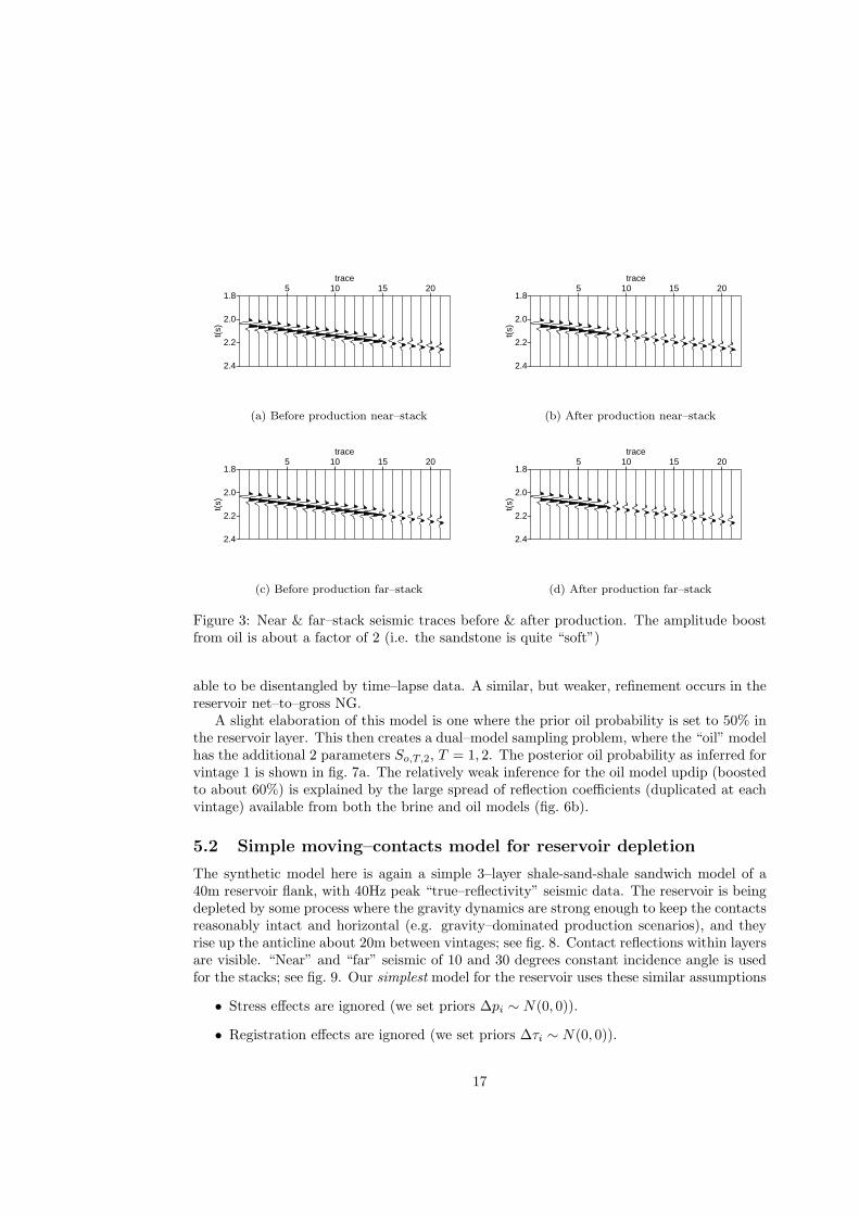
Figure 3: Near & far–stack seismic traces before & after production. The amplitude boostfrom oil is about a factor of 2 (i.e. the sandstone is quite “soft”)
able to be disentangled by time–lapse data. A similar, but weaker, refinement occurs in thereservoir net–to–gross NG.
A slight elaboration of this model is one where the prior oil probability is set to 50% inthe reservoir layer. This then creates a dual–model sampling problem, where the “oil” modelhas the additional 2 parameters So,T,2, T = 1, 2. The posterior oil probability as inferred forvintage 1 is shown in fig. 7a. The relatively weak inference for the oil model updip (boostedto about 60%) is explained by the large spread of reflection coefficients (duplicated at eachvintage) available from both the brine and oil models (fig. 6b).
5.2 Simple moving–contacts model for reservoir depletion
The synthetic model here is again a simple 3–layer shale-sand-shale sandwich model of a40m reservoir flank, with 40Hz peak “true–reflectivity” seismic data. The reservoir is beingdepleted by some process where the gravity dynamics are strong enough to keep the contactsreasonably intact and horizontal (e.g. gravity–dominated production scenarios), and theyrise up the anticline about 20m between vintages; see fig. 8. Contact reflections within layersare visible. “Near” and “far” seismic of 10 and 30 degrees constant incidence angle is usedfor the stacks; see fig. 9. Our simplest model for the reservoir uses these similar assumptions
• Stress effects are ignored (we set priors ∆pi ∼ N(0, 0)).
• Registration effects are ignored (we set priors ∆τi ∼ N(0, 0)).
17
rock trend prior distributions
2000 2200 2400 2600 2800 3000 32001.9
2.0
2.1
2.2
2.3
2.4
2.5
2.6
vp(m/s)
rho(
gm/c
c)
(a) Prior rock–physics scatterplots
reservoir drained−zone posterior
2000 2200 2400 2600 2800 3000 32001.9
2.0
2.1
2.2
2.3
2.4
2.5
2.6
vp_eff(m/s)
rho
_e
ff(m
/s) vp_eff, rho_eff vintage 2
vp_eff, rho_eff vintage 1
(b) Posterior scatterplots including saturation and NGeffects (reservoir properties are effective)
Figure 4: Scatterplots from rock physics models in centre of depleted region (trace 10). Blueis bounding shale, green is brine–referenced sand, red is full-saturation sand.
• Rock mixing in the reservoir is modelled with NG∼ N(0.9, 0.22).
• Unknown saturation in the reservoir is modelled with So,T,2 ∼ N(0.7, 0.42) (vintagesT = 1, 2, layer 2).
• The gas–oil and oil-brine contacts are given 20m uncertainty in the prior for bothvintages (but the mean is raised 20m for the vintage 2 contact).
• Peak–signal to noise RMS is set at about 5:1.
Fig. 10 shows show typical realisations for contact–controlled fluids for each vintage.Fig. 11 shows typical spaghetti plots of model–sample fits to the seismic traces, illustratingthe goodness of fit for the near stack. Fig. 12 shows typical estimations of hydrocarbonsaturation for each vintage. These saturations are “layer–upscaled”, i.e. the saturations arediscounted by the fractional thickness containing the salient fluid, so they naturally taperoff as the contact surface pinches out.
18
seismic amplitudes
1.9
1.95
2
2.05
2.1
2.15
2.2
2.25
2.3
2.35
t
(a) Before production near–stack spaghetti plots
seismic amplitudes
1.9
1.95
2
2.05
2.1
2.15
2.2
2.25
2.3
2.35
t
(b) After production near–stack spaghetti plots
seismic amplitudes
1.9
1.95
2
2.05
2.1
2.15
2.2
2.25
2.3
2.35
t
(c) Before production far–stack spaghetti plots
seismic amplitudes
1.9
1.95
2
2.05
2.1
2.15
2.2
2.25
2.3
2.35
t
(d) After production far–stack spaghetti plots
Figure 5: Near & far–stack seismic traces and model–sample traces before & after production(usually called “spaghetti plots”). Close inspection shows ensembles of synthetics (black)for each model underneath the red “true” data.
19
oil saturation median
0 5 10 15 200.0
0.2
0.4
0.6
0.8
1.0
trace
med
ian
S_o
il
(a) Median inferred oil saturation (red=”before”,green=”after”)
reservoir posterior S_oil
0.0 0.2 0.4 0.6 0.8 1.0 1.20
200
400
600
800
1000
1200
1400
1600
S_oil
coun
t
(b) Oil saturation histograms at 3 locations. Red = up-dip,before; Blue = downdip,before; Magenta = swept–zone,before; Green = swept–zone,after;
Figure 6: Inferred oil–saturation statistics.
20
MAP_oil_probability
0 5 10 15 200.0
0.2
0.4
0.6
0.8
1.0
trace
prob
.
(a) Median inferred oil probability
reflection_coefficient
−0.3 −0.2 −0.1 0.0 0.1 0.2 0.30
500
1000
1500
2000
R_pp
count
downdip-brineupdip-oil
(b) Updip reflection coefficient histograms for the brineand oil models compared to the “truth–case” reflectionspikes
Figure 7: Diagnostic plots for the 2–model model–averaging run.
0 2 4 6 8 10 12 14 16
sample/trace
2
2.02
2.04
2.06
2.08
2.1
2.12
2.14
2.16
2.18
2.2
2.22
2.24
2.26
2.28
2.3
t
(a) Before production (vintage 1)
0 2 4 6 8 10 12 14 16
sample/trace
2
2.02
2.04
2.06
2.08
2.1
2.12
2.14
2.16
2.18
2.2
2.22
2.24
2.26
2.28
2.3
t
(b) After production (vintage 2)
Figure 8: Contacts–based 3–layer reservoir anticline model (see section 5.2) showing bound-ing shales (brown), and reservoir fluids (orange=gas, red=oil, blue=brine) before & afterproduction. Both contacts rise slightly between the two model vintages shown.
21
1.9
2.1
2.3
t(s)
5 10 15trace
(a) Before production near–stack
1.9
2.1
2.3
t(s)
5 10 15trace
(b) After production near–stack
1.9
2.1
2.3
t(s)
5 10 15trace
(c) Before production far–stack
1.9
2.1
2.3
t(s)
5 10 15trace
(d) After production far–stack
Figure 9: Near & far–stack seismic traces before & after production. The contacts beforeand after production in this naive model are quite visible.
22
0 100 200 300 400 500 600 700 800
sample/trace
1.98
2
2.02
2.04
2.06
2.08
2.1
2.12
2.14
2.16
2.18
2.2
2.22
2.24
2.26
2.28
2.3
t
(a) Vintage 1 fluid position samples
0 100 200 300 400 500 600 700 800
sample/trace
1.98
2
2.02
2.04
2.06
2.08
2.1
2.12
2.14
2.16
2.18
2.2
2.22
2.24
2.26
2.28
2.3
t
(b) Vintage 2 fluid position samples
Figure 10: “Unrolled” model uncertainty images (stacks of 50 samples per trace from theposterior) showing fluid contact uncertainties in time for each vintage.
seismic amplitudes
1.95
2
2.05
2.1
2.15
2.2
2.25
2.3
t
(a) Before production near–stack spaghetti plots
seismic amplitudes
1.95
2
2.05
2.1
2.15
2.2
2.25
2.3
t
(b) After production near–stack spaghetti plots
Figure 11: Near–stack seismic traces and model–sample traces before & after production.
23
0 2 4 6 8 10 12 14 160.0
0.2
0.4
0.6
0.8
1.0
trace
S_
ga
s(u
psca
led
)
(a) Gas saturation
0 2 4 6 8 10 12 14 160.0
0.2
0.4
0.6
0.8
1.0
trace
S_
oil(
up
sca
led
)
(b) Oil saturation
Figure 12: Inferred oil and gas–saturation profiles across the reservoir. The three curves areP16,P50,P84 quantiles of upscaled saturation, for each vintage: red=“before”, green=“after”production. The updip–moving slug of fluids is clearly evident between the two vintages.
24
5.3 Simple stress–dependent model
This model is essentially the same as the model of section 5.1, except stress effects aremodelled in a representative cartoon–like way to illustrate the machinery. Here, the centralthird of the model is swept of oil, piston–like, from S=70% to 10% saturation.
To model pore–pressure effects, the in–situ pore–pressure change from vintage 1 to vin-tage 2 is set as a ramping function from -1 to 1 (in some suitable set of scaled units) goingfrom left to right across the image (‘producer’ to ‘injector’, see fig. 14a). The referencelayer is the reservoir, and the 3 stress correlation coefficients (equation 1) are taken asU1,2 = −0.1, U2,2 = 1, U3,2 = −0.05, roughly to induce the expected opposite strain statesin the bounding shales (the over/underburden near producers goes weakly into extension).In these pressure units,the stress–path–coefficients of shale and sandstone are set at -200m/sand -180m/s respectively. Fig 13 depicts the model.
With areally–constant constant oil saturation, the expected amplitudes showing the ef-fects of stress are shown in fig. 14b. Fig 14c show the effects of the swept–area saturationchange only, and fig. 14d shows both effects combined. Fig. 15 shows the effects of stress ontypical vp vs ρ scatterplots at the two extremes of the pore–pressure ramp. The effect onthe bounding shale is less visible chiefly because of the stress correlation coefficient of 0.1.
For inversion, the model is set up roughly as before. The priors for the reservoir layerare chosen as NG∼ Ntr(0.9, 0.22), Poil = 1, Soil,vintage=1,2 ∼ Ntr(0.55, 0.42), and ∆pT ∼N(∆pT,true, 0.22), i.e. the pore pressure prior is centered on the “truth–case” with about40% relative slack. In actual real inversions, given how benign pressure responses typicallyare to reservoir unknowns, we might hope to be able to set the prior distribution for pressurerather more tightly than this.
Again, the most interesting plot is probably inferred oil saturation from the time–lapsemodel. The median saturation from the ensemble of samples is shown in Fig. 16.
This is roughly the same picture as before. Note that the inference on saturation in theswept zone is again stronger than up/downdip, but not as strong as the case with no pore–pressure effects, so this is likely due to the confusing effects of stress. It is reassuring thatthe pore–pressure effect can apparently be removed from the data even when the movementof saturations is not immediately evident from amplitude differences. This is provided, ofcourse, the stress effects model and its associated parameters are approximately correct.
25
0 2 4 6 8 10 12 14 16 18 20 22
sample/trace
1.95
2
2.05
2.1
2.15
2.2
2.25
2.3
2.35
t
(a) Oil saturation, vintage 1
0 2 4 6 8 10 12 14 16 18 20 22
sample/trace
1.95
2
2.05
2.1
2.15
2.2
2.25
2.3
2.35
t
(b) Oil saturation, vintage 2
0 2 4 6 8 10 12 14 16 18 20 22
sample/trace
1.95
2
2.05
2.1
2.15
2.2
2.25
2.3
2.35
t
(c) Effective p–impedance Z eff, vintage 1
0 2 4 6 8 10 12 14 16 18 20 22
sample/trace
1.95
2
2.05
2.1
2.15
2.2
2.25
2.3
2.35
t
(d) Effective p–impedance Z eff, vintage 2
Figure 13: Cartoon 3–layer model for stress effects
26
5 10 15 20−1.0
−0.5
0.0
0.5
1.0
delta
_por
e_pr
essu
re
(a) Change in pore–pressure profile from vintage 1 to vintage 2, scaledpressure units
1.9
2.1
2.3
5 10 15 20
(b) Stress–only effect on amplitudes from vintage 1 to vintage 2, near–stack
1.9
2.1
2.3
5 10 15 20
(c) Saturation–only effect
1.9
2.1
2.3
5 10 15 20
(d) Combined effects
Figure 14: Effects of saturation and pore pressure change for simple stress–dependent model.
27
2200 2400 2600 2800 3000 3200 34002.0
2.1
2.2
2.3
2.4
2.5
2.6
vp(m/s)
dens
ity(g
m/c
c)
Figure 15: vp vs ρ prior–model scatterplots from overburden shale (squares) and reservoirsand (circles) at producer (red) and injector (green), showing effect of pore pressure change.
28
0 5 10 15 200.2
0.3
0.4
0.5
0.6
0.7
0.8
0.9
trace
me
dia
n S
_o
il
before production
after production
updip downdipswept-zone
(a) Median inferred oil saturation (red=”before”,green=”after”)
0.0 0.2 0.4 0.6 0.8 1.0 1.20
200
400
600
800
1000
1200
1400
1600
S_oil
co
un
t
downdip, before
(trace 20) updip, before (trace 0)
swept-zone, before(trace 10)
swept-zone, after (trace 10)
production
(b) Oil saturation histograms at 3 locations. Red =updip (trace1), before; Blue = downdip(trace 21), be-fore; Magenta = swept–zone (trace 10),before; Green= swept–zone,after;
Figure 16: (a) and (b), inferred oil–saturation statistics, for model with pore–pressure priorcentered on truth case (∆pT ∼ N(∆pT,true, 0.22)). (c) shows quantiles from inferred pore–pressure posterior with this prior. (d) Inferred pore–pressure posterior quantiles acrossmodel if a broad, “flat” prior is used: ∆pT ∼ N(0, 0.72).
29
6 Discussion
The present implementation implements a reasonable amount of the modelling conceptsone would like in a post–imaging AVO inversion code for time–lapse data that bypasses 3Dstress and flow simulation. The relatively simple physics for stress and saturation effects andseismic response make for an extremely fast forward model that can be used in demandingstatistical frameworks like MCMC. There will always be concerns about whether the modelsare adequate for complex reservoir responses, but it is difficult to argue the case for moresophisticated models without requiring in turn that the problem requires a complex 3Dcoupled geomechanical, flow and wave equation simulation.
At present, the code functionality has been tested chiefly on synthetic cases with datagenerated from the same forward engine as the inversion kernel. Such tests are not intendedto be compelling marketing exercises, but serve at least as minimum due–diligence in codetesting and proof–of–concept. They provide also instances of how much refinement in pos-terior parameters one might hope for in “ideal” cases where the geometry and rock physicsare representative, and the statistical assumptions reasonable or at least benign. Certainresults emphasise the forensic value of time–lapse data in focusing down to a few explanatoryvariables for regions with significant amplitude changes. They also illumine cases where theseismic data is unhelpful in refining reservoir parameters. I normally regard these examplesas “upper bounds” on inferences, as real data usually have confounding factors or physicswhich make inferences based on the usual ideal assumptions more dubious.
This trace–based inversion produces samples from a “local” posterior distribution usinglocal seismic data and local layer parameters. No “transverse” coupling of parameters (spa-tial continuity) is built into the prior model, but transverse trends are certainly controllablevia the model prior. Three–dimensional model realisations will not naturally ensue fromindependent samples from these distributions stitched together: a possible way to inducetransverse spatial continuities via some post–processing is discussed in [6]. One relativelygood reason for confining the model to trace–local sampling, as opposed to a large, spatiallycoupled model is this. Spatially coupled geostatistical models (e.g Gaussian Markov randomfields) have the property of reducing the number of effective degrees of freedom in the model,which makes the posterior distributions tighter. But the noise model for imaged 3D seis-mic data should incorporate lateral correlation (e.g. over scales at least as large as Fresnelzones), which reduces the effective information content of the data. The two effects operateto cancel each other, but the price that has been paid is usually a very large increase in theruntime costs of the model, and an even worse penalty in MCMC efficiency measures. Theshape of the local–posterior obtained from a trace–independent model is often a reasonableestimate of a local marginal–posterior distribution obtained by conceptually integrating outall the non–local variables in a large coupled model.
Transverse physical consistency of flow–dynamical variables like pressure and saturationis largely dependent on sensible prior distributions, since we do not use any form of flowsimulation. The same remark, mutatis mutandis, applies to stress. The general implication isthat the machinery rests on the idea that the seismic amplitudes have sufficient informationcontent, supplemented with simple stress and saturation models, to identify the main areasof fluid movement in the model. Clearly there will be cases where this is not true (noisyseismic, low porosity rocks etc), but an appreciable fraction of such cases are those wherethe value of 4D monitors are questionable, precisely because they must rely so heavily on
30
flow simulation. Like many technologies in the oil industry, I expect there will be caseswhere simple, fast, leading–order modelling yields useful results, but once second–orderand coupled effects become appreciable, the prospects for full inference with estimates ofuncertainty become rather more remote.
7 Conclusion
This paper describes an extension of the Delivery seismic inversion code suitable for usein time–lapse problems where the modelling assumptions involved are reasonable. Theseinclude “directionally linearised” elasticity responses driven by pore pressure change, simpleGassmann–like dependencies for saturation effects, and 1D convolutional modelling for theseismic response. The code provides a range of statistical outputs, chiefly local MAP pointsestimated by optimisation sweeps over the (possibly multi–modal) candidate fluid models,and samples from the Bayesian posterior distribution generated by an MCMC algorithm.
A deal of modelling effort is required to set up suitable prior distributions for the modellayers and rock physics, but valuable oil and gas assets worthy of repeated time lapse surveysusually warrant such effort. The synthetic inversion test cases described show characteristicestimates of how much refinement in reservoir properties is likely to occur in cases withgood signal to noise ratios. These refinements are often sharper in areas where the imagedreflectivities change appreciably, since the differential measurements may be explicable byonly certain variables. Tests on field data will be discussed in a later publication.
31
Appendices
Appendix 1: Formats
Strawman XML input format
The input XML format requires only modest changes to allow the specification of multipleseismic data. Extra chunks for the elasticity coefficients are needed. Figures 17,18,19 belowhighlight the new entries in the XML required to run time–lapse models.
The formats are controlled by the XSD schema as before, but the changes required fromexisting Delivery formats roughly comprise
• A high level format entry: inversion/time lapse format
• Vintage tags for each inversion/seismic data/stack
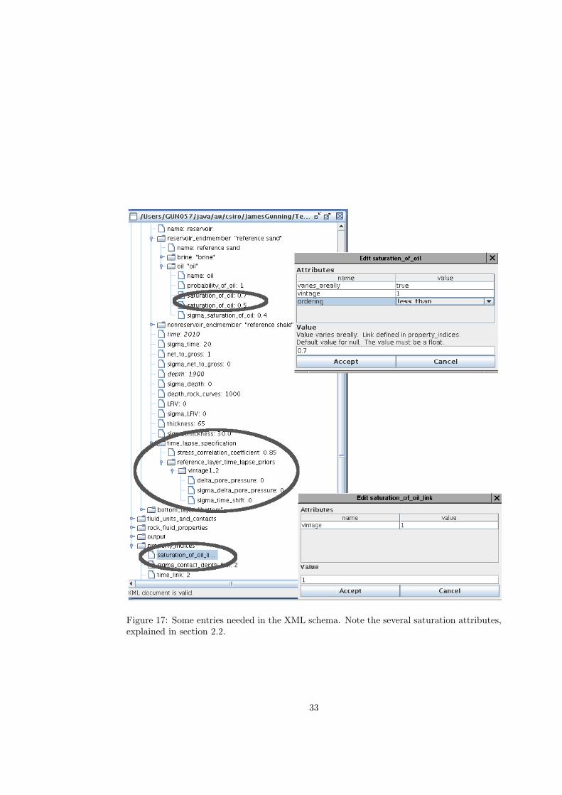
• Each inversion/model description/layer needs a time lapse specification. Alllayers need astress correlation coefficient (as defined by eqn (1)), additionally, the reference–depth layer needs a full reference layer time lapse priors field
• Any hydrocarbon fluid entry like inversion/model description/*layer/reservoir
endmember/oil/saturation of oil, for example, should set the attribute “vintage”.Ditto for sigma saturation of oil. Missing vintage attributes will be taken to meanthe supplied number applies to all vintages.
• If contact–modelling is used, a fluid–unit must specify a sequence of vintage entriesunderinversion/fluid units and contacts/fluid unit/, with a sequence of applicablecontact entries for all the contacts modelled at each vintage. Each contact is identifiedby type, and requires a depth entry which has attributes specifying whether it variesareally, the vintage number, and vintage–ordering criterion for the depth. The priorsfor depth and sigma depth for each permissible contact type (GO,OB etc) then applyfor that stated vintage.
• The rock physics section must be augmented with the elementsinversion/rock fluid properties/rock properties/*reservoir endmember-
/stress path coefficients/vintage1 N where vintage1 N specifies the stress pathcoefficients for the stress–regime change from vintage1 to vintage N.
• Trace–variable model elements in inversion/property indices are entered on a pervintage basis for elements like contact depth link, sigma contact depth link,
saturation of oil link etc, where the vintage attribute must be set to indicatewhich vintage model parameter is set by the nominated trace block. Variable contactsuse the additional attribute type (e.g. OB) to identify the correct model property (i.e.the correct contact and the correct vintage).
32
Figure 17: Some entries needed in the XML schema. Note the several saturation attributes,explained in section 2.2.
33
Figure 18: More new entries needed in the XML schema
34
Figure 19: Even more entries needed in the XML schema
35
Output format
At present, for writing binary–format “realisation.su” output files for holding either sampleor “MAP” models, delivery uses a big–endian SU format (no ebdic header), with some wordswith reserved meanings:
• “mark” realisation number
• “duse” contains version encodings (for legacy file compatibility)
• “sdepth” for format compression in simpler models (a bit–mask of “features”)
Fields like ep,cdp,tracl,tracr,fldr,sx,sy,gx,gy carry useful survey info and are inherited fromthe first seismic stack1. For a time–lapse format, we propose to retain a SU header, concate-nate successive vintages of “samples” down the trace, and make the length of each vintagesub–block depend on the (maximum) number of stacks. We use two more header words toencode:
• “nvs” number of vintages Nv
• “nhs” the maximum number of stacks Ns per vintage (not counting difference stacks).
The number of stacks available may vary over vintages, but a fully general arrangementis hard to impose upon the SU header format. The “rectangular” format above usesonly 2 extra header words: “missing” stack fields can simply default to some null value.See Fig. 20. There are Nl layers in the model. At present, there are NPS = 2 proper-
240B header
stack-dependent entries R_pp, Rpp_fc, total size NlNs for each of R_pp, R_pp_fc
ns samples
Nl entries like NG, vp_eff Nl+1 times
Vintage 1 Vintage 2 Vintage 3
Ns=3 stacks
.... ........ .... ...........
NV=3 vintages
Nl layers
Figure 20: Speculative Delivery4D output format
ties R pp,R pp fc (pp reflection coefficient at layer boundaries, and reflection coefficient atfluid contacts respectively, or their ps equivalents if the stack attribute isPSdata = true)which require multi–stack output. These need NlNPS slots available in the output SUfile, per vintage. A typical run will dump, for each vintage, a sequence of NF propertiesd,LFIV,NG,vp m,vs m,rho m,vp s...t,t base in blocks of size Nl, except for i) the lastt-block, of size Nl + 1, and ii) the R pp,R pp fc blocks, of size NlNs. This list is available
1In a sensible project, they should be shared across all stacks of course
36
from the --BHPcommand flag. For convenience, the number of samples ns is the SU propertiesfile is then
ns = Nv(1 + Nl(NF − 1 − NPS + NsNPS)
and conversely, the number of layers computed from the number of samples ns is
Nl =ns/Nv − 1
NF − 1 + NPS(Ns − 1).
Additional “property blocks” delta p and time shift will be available for ∆p and ∆τ ,these being logically set at zero for vintage 1, and are identical for all layers in a vintage.
For fluid–contact models, for each vintage, properties like d fc,t fc are dumped intoa block of size Nl, in an unrolled sequence corresponding to nested loops over fluid–unit,contact–number respectively. The block is zero–padded. The total number of contacts pervintage must not exceed Nl (this is checked at XML parsing when running).
References
[1] James Gunning and Michael Glinsky. Delivery: an open-source model-based Bayesianseismic inversion program. Computers and Geosciences, 30(6):619–636, 2004.
[2] James Gunning. Delivery website: http://www.csiro.au/products/Delivery.html.Substantially updated pdfs of the important papers and the code may be obtained here.
[3] R Calvert. 4D technology: where are we, and where are we going? GEOPHYSICALPROSPECTING, 53(2):161–171, MAR 2005.
[4] Colin M. Sayers. Geophysics Under Stress : SEG/EAGE DISC 2010. SEG, 2010. ISBN978-1-56080-210-5.
[5] Paul Hatchell and Stephen Bourne. Rocks under strain: Strain-induced time-lapse timeshifts are observed for depleting reservoirs. The Leading Edge, 24(12):1222–1225, 2005.
[6] James G. Gunning, Michael E. Glinsky, and Chris White. DeliveryMassager: a tool forpropagating seismic inversion information into reservoir models. in press, Computersand Geosciences, 2007.