Page 1 of 18 Program: Conservation Applications of LiDAR Data http://tsp.umn.edu/lidar Funder: Environment and Natural Resources Trust Fund Module: Hydrologic Applications Instructor: Sean Vaughn, DNR GIS Hydrologist Funded by: Minnesota’s Clean Water Fund Exercise: DEM Display Objectives Learn the basics of setting Environment Settings to control raster analysis and processing outputs. Demonstrate methods to display a DEM and associated raster products for the purpose of hydrography identification and delineation. Exercise & Data Location: Root Folder for this exercise = %root folder%\ = C:\Temp\_sevaughn_LiDAR\DEM_DISPLAY Root Folder for this exercise = %root folder%\ = Flash_Drive\_sevaughn_LiDAR\DEM_DISPLAY
Transcript
Page 1 of 18
Program: Conservation Applications of LiDAR Data http://tsp.umn.edu/lidar
Funder: Environment and Natural Resources Trust Fund
Module: Hydrologic Applications
Instructor: Sean Vaughn, DNR GIS Hydrologist
Funded by: Minnesota’s Clean Water Fund
Exercise: DEM Display
Objectives
Learn the basics of setting Environment Settings to control raster analysis and processing outputs.
Demonstrate methods to display a DEM and associated raster products for the purpose of hydrography identification and delineation.
Exercise & Data Location:
Root Folder for this exercise = %root folder%\ = C:\Temp\_sevaughn_LiDAR\DEM_DISPLAY
Root Folder for this exercise = %root folder%\ = Flash_Drive\_sevaughn_LiDAR\DEM_DISPLAY
Page 2 of 18
ArcMap Setup The set up of ArcMap with the proper toolbars, extensions, and environmental settings is critical for this exercise. In addition to using the functionality of these various ArcMap capabilities we want you to understand how to: locate, load, and setup these toolbars, extensions, and environmental settings. You can retain these instructions for future reference.
1. Data Location. All data is stored on your PC at root directory:
%root folder%:\dem_display_DATA.
2. Open your GIS software. Start by opening ArcMap.
3. Connect to Folder. Use Connect to Folder to establish quicker data mapping.
a. Using ArcMap and or ArcCatalog map to the folder containing the course data.
Location: %root folder%\
4. Load the Base DEM. Using ArcMap or ArcCatalog (your preference), load the base Digital Elevation Model (DEM) [DEM03] into the ArcMap Table of Contents.
Location: %root folder%\:dem_display_data.
Page 3 of 18
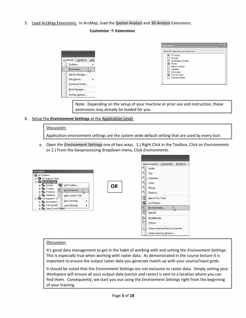
5. Load ArcMap Extensions. In ArcMap, load the Spatial Analyst and 3D Analyst Extensions.
Customize Extensions
Note: Depending on the setup of your machine or prior use and instruction, these extensions may already be loaded for you.
6. Setup the Environment Settings at the Application Level.
Discussion:
Application environment settings are the system wide default setting that are used by every tool.
a. Open the Environment Settings one of two ways. 1.) Right Click in the Toolbox, Click on Environments or 2.) From the Geoprocessing dropdown menu, Click Environments.
Discussion:
It’s good data management to get in the habit of working with and setting the Environment Settings. This is especially true when working with raster data. As demonstrated in the course lecture it is important to ensure the output raster data you generate match up with your source/input grids.
It should be noted that the Environment Settings are not exclusive to raster data. Simply setting your Workspace will ensure all your output data (vector and raster) is sent to a location where you can find them. Consequently, we start you out using the Environment Settings right from the beginning of your training.
OR
Page 4 of 18
There are four levels of Environment Settings that form a hierarchy: 1. application, 2. tool, 3. model, and 4. model process. In this hierarchy, all levels contain the same environment variables and have the same effect on output results. The levels differ only in how you access and set them. However, Environment Settings are passed down to the next level. These passed‐down Environment Settings can be overridden at each succeeding level.
We feel more comfortable establishing the Environment Settings at the tool level even if previously set at the application level. However, for the following steps in this exercise you will be asked to set the Environment Settings at both the application and tool levels.
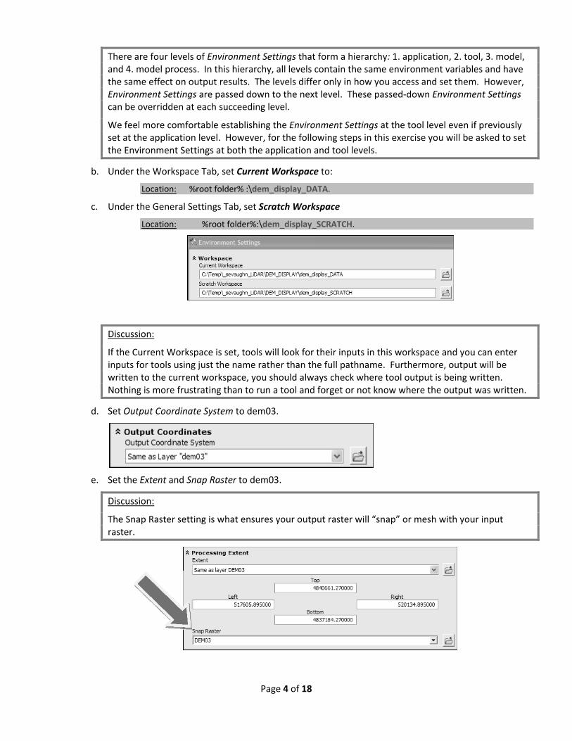
b. Under the Workspace Tab, set Current Workspace to:
Location: %root folder% :\dem_display_DATA.
c. Under the General Settings Tab, set Scratch Workspace
Location: %root folder%:\dem_display_SCRATCH.
Discussion:
If the Current Workspace is set, tools will look for their inputs in this workspace and you can enter inputs for tools using just the name rather than the full pathname. Furthermore, output will be written to the current workspace, you should always check where tool output is being written. Nothing is more frustrating than to run a tool and forget or not know where the output was written.
d. Set Output Coordinate System to dem03.
e. Set the Extent and Snap Raster to dem03.
Discussion:
The Snap Raster setting is what ensures your output raster will “snap” or mesh with your input raster.
Page 5 of 18
Note: The Extent will state “As Specified Below” the next time you open the Environment Settings.
f. Set the Raster Analysis Settings to dem03.
7. Add the Land Facet Analysis Tool Bar.
a. Customize Toolbars Land Facet Analysis
8. Save/Save As your ArcMap project to DEM_display
Name: DEM_display
Location: %root folder%:\dem_display_PROJECT
Note: The Land Facet Corridor Designer can be downloaded at: http://corridordesign.org/downloads
Page 6 of 18
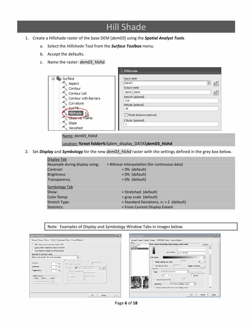
Hill Shade 1. Create a Hillshade raster of the base DEM [dem03] using the Spatial Analyst Tools.
a. Select the Hillshade Tool from the Surface Toolbox menu.
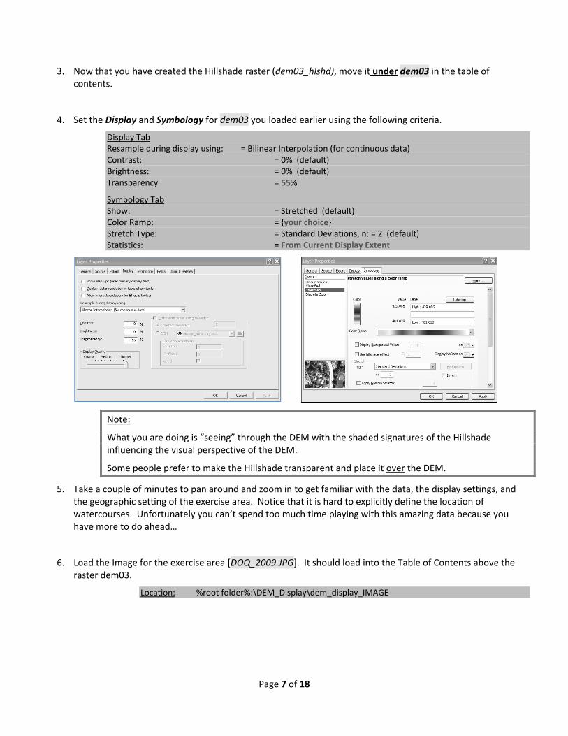
Symbology Tab Show: = Stretched (default) Color Ramp: = {your choice} Stretch Type: = Standard Deviations, n: = 2 (default) Statistics: = From Current Display Extent
Note:
What you are doing is “seeing” through the DEM with the shaded signatures of the Hillshade influencing the visual perspective of the DEM.
Some people prefer to make the Hillshade transparent and place it over the DEM.
5. Take a couple of minutes to pan around and zoom in to get familiar with the data, the display settings, and the geographic setting of the exercise area. Notice that it is hard to explicitly define the location of watercourses. Unfortunately you can’t spend too much time playing with this amazing data because you have more to do ahead…
6. Load the Image for the exercise area [DOQ_2009.JPG]. It should load into the Table of Contents above the raster dem03.
7. Turn the DOQ on and off repeatedly to see how the topography looks without the hill shaded DEM. Take a moment to toggle back and forth to see how much topography is visible in the DEM compared to what the high quality DOQ offers.
8. Turn off dem03.
9. In the Table of Contents Move the DOQ under dem03_hlshd in the Table of Contents and set dem03_hlshd to 60% Transparent.
Page 9 of 18
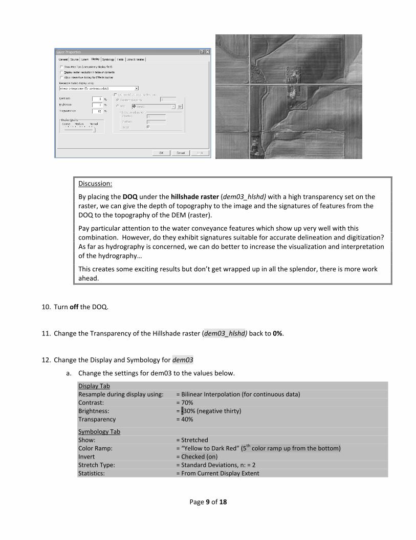
Discussion:
By placing the DOQ under the hillshade raster (dem03_hlshd) with a high transparency set on the raster, we can give the depth of topography to the image and the signatures of features from the DOQ to the topography of the DEM (raster).
Pay particular attention to the water conveyance features which show up very well with this combination. However, do they exhibit signatures suitable for accurate delineation and digitization? As far as hydrography is concerned, we can do better to increase the visualization and interpretation of the hydrography…
This creates some exciting results but don’t get wrapped up in all the splendor, there is more work ahead.
10. Turn off the DOQ.
11. Change the Transparency of the Hillshade raster (dem03_hlshd) back to 0%.
12. Change the Display and Symbology for dem03
a. Change the settings for dem03 to the values below.
Symbology Tab Show: = Stretched Color Ramp: = “Yellow to Dark Red” (5th color ramp up from the bottom) Invert = Checked (on) Stretch Type: = Standard Deviations, n: = 2 Statistics: = From Current Display Extent
Page 10 of 18
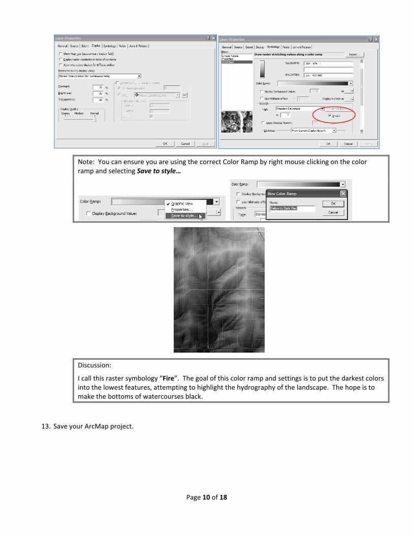
Note: You can ensure you are using the correct Color Ramp by right mouse clicking on the color ramp and selecting Save to style…
Discussion:
I call this raster symbology “Fire”. The goal of this color ramp and settings is to put the darkest colors into the lowest features, attempting to highlight the hydrography of the landscape. The hope is to make the bottoms of watercourses black.
13. Save your ArcMap project.
Page 11 of 18
TPI Raster Creation Now we will now explore a method of indentifying the hydrography in the DEM with more intensity and definition using a special output raster with simple display and symbology settings.. We will do this through a multistep process using a free ArcMap Toolbox called Land Facet Corridor Tools. From that extension we will employ the Land Facet Analysis tool which contains the Topographic Position Index (TPI) functionality.
TPI
TPI is the difference between a cell’s elevation value and the average elevation of the neighborhood around that cell.
Positive values mean the cell is higher than its surroundings while
Negative values mean it is lower.
TPI Evolution and Availability
Andrew Weiss
First presented at the 2001 ESRI International User Conference. Jeff Jenness , Wildlife Biologist, GIS Analyst, Jenness Enterprises.
Originally wrote the code in Avenue for ArcView 3.3.
Available for ArcGIS 10 at: http://corridordesign.org/ Thomas Dilts , Research Scientist, University of Nevada, Reno.
Migrated the TPI functionality to an ArcGIS toolbox.
Available for ArcGIS 9.x at: http://arcscripts.esri.com/details.asp?dbid=15996
1. Make a Topographic Index Raster.
Open the Land Facet Analysis Toolbar Topographic Position Index Tools Calculate TPI Raster.
Docked Tool Bar
Floating Tool Bar
Toolbar Menu
Page 12 of 18
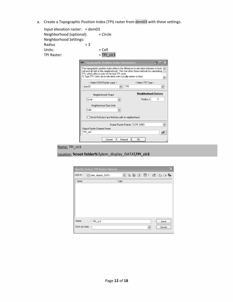
a. Create a Topographic Position Index (TPI) raster from dem03 with these settings.
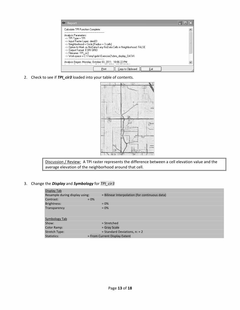
2. Check to see if TPI_cir3 loaded into your table of contents.
Discussion / Review: A TPI raster represents the difference between a cell elevation value and the average elevation of the neighborhood around that cell.
Symbology Tab Show: = Stretched Color Ramp: = Gray Scale Stretch Type: = Standard Deviations, n: = 2 Statistics: = From Current Display Extent
Page 14 of 18
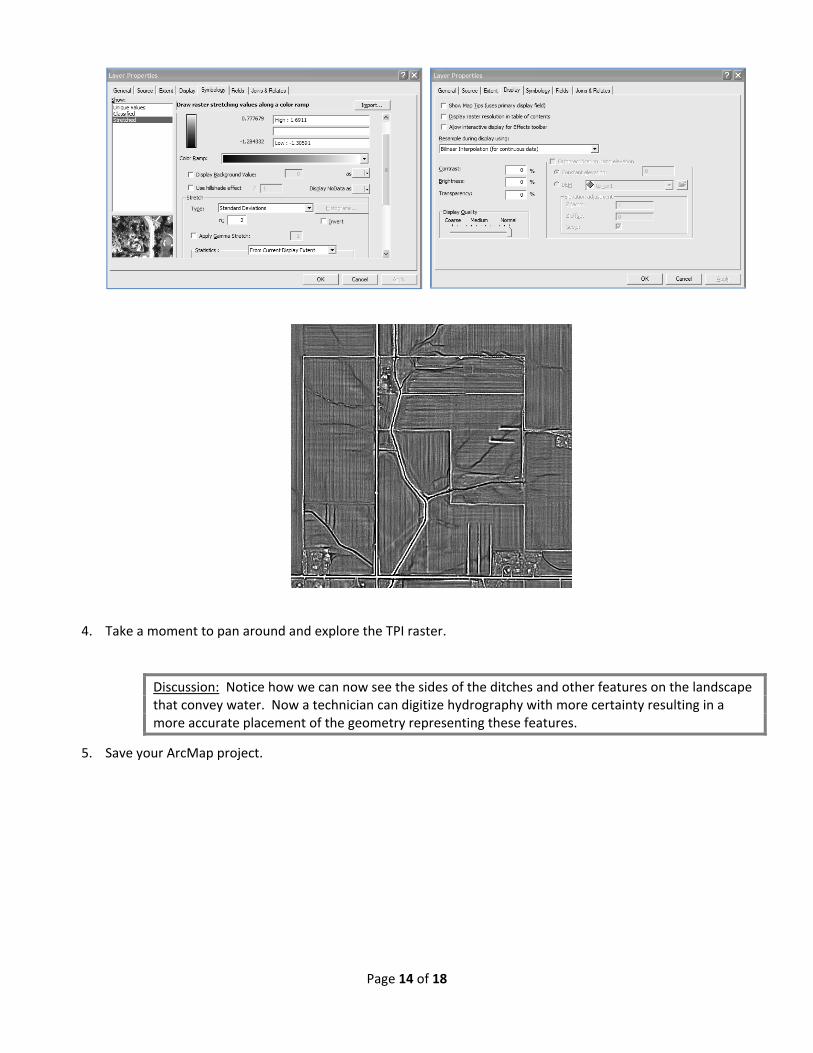
4. Take a moment to pan around and explore the TPI raster.
Discussion: Notice how we can now see the sides of the ditches and other features on the landscape that convey water. Now a technician can digitize hydrography with more certainty resulting in a more accurate placement of the geometry representing these features.
5. Save your ArcMap project.
Page 15 of 18
TPI Raster Integration 1. In your table of contents Turn off dem03.
2. Turn on dem03_hlshd.
a. Ensure the Display for dem03_hlshd is set to “0%” transparency.
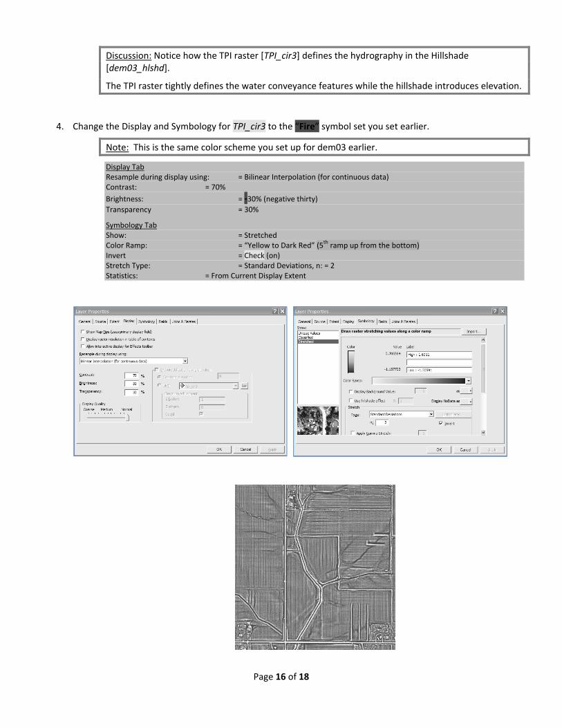
3. Change the Display and Symbology again for TPI_cir3 to:
Symbology Tab Show: = Stretched Color Ramp: = “Yellow to Dark Red” (5th ramp up from the bottom) Invert = Check (on) Stretch Type: = Standard Deviations, n: = 2 Statistics: = From Current Display Extent
Page 17 of 18
Discussion: When you are working in areas with such minimal elevation as in this exercise data, the roads and ditch banks “pop” with this “Fire” color scheme, making for easy interpretation of the features that convey water on the landscape. Like our earlier TPI illustration, the technician only needs to concentrate on the features in black for digitizing the hydrography, resulting in a more accurate final digitized product.
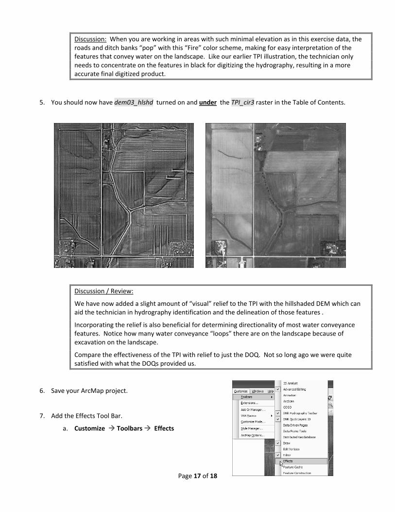
5. You should now have dem03_hlshd turned on and under the TPI_cir3 raster in the Table of Contents.
Discussion / Review:
We have now added a slight amount of “visual” relief to the TPI with the hillshaded DEM which can aid the technician in hydrography identification and the delineation of those features .
Incorporating the relief is also beneficial for determining directionality of most water conveyance features. Notice how many water conveyance “loops” there are on the landscape because of excavation on the landscape.
Compare the effectiveness of the TPI with relief to just the DOQ. Not so long ago we were quite satisfied with what the DOQs provided us.
6. Save your ArcMap project.
7. Add the Effects Tool Bar.
a. Customize Toolbars Effects
Page 18 of 18
8. Use the “Swipe Layer” to see how the TPI raster lines up with the original DEM and the DOQ.
9. Explore the raster’s.
10. Save your project – END
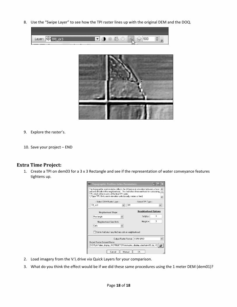
ExtraTimeProject:1. Create a TPI on dem03 for a 3 x 3 Rectangle and see if the representation of water conveyance features
tightens up.
2. Load imagery from the V:\ drive via Quick Layers for your comparison.
3. What do you think the effect would be if we did these same procedures using the 1 meter DEM (dem01)?