Demand and Supply AnalysisCompiled by Jyoti P. Sarkar

A. DEMAND ANALYSIS: I. Concepts• Meaning—Demand, DD= Desire + Ability to pay + Willingness to pay

• Quantity demanded- Amount of a good that buyers are willing and able to purchase at a particular period of time.

• Demand Schedule- a tabular representation of the relationship between quantity demanded and its determinant (here, price) other determinants reaming constant at a particular period of time.

• Demand Curve- a graphical representation of the relationship between quantity demanded and its determinant (here, price) other determinants reaming constant at a particular period of time.

Demand Schedule Demand Curve

L.S.Raheja College of Commerce and Arts (SFC)

Price of Coffee ( in ₹ ) Quantity Demanded(Qx = 100 – 10 Px)

1 90

2 80

3 70

II. Individual demand

Demand of one individual consumers for the product at different possible prices at a given point of time.

Individual Demand Curve

Individual Demand curve is downward sloping

Reason: Income effect and substitution effect

III. Law of Demand

According to the Law of Demand,there is and inverse relationshipbetween price and quantitydemanded for a commodity, all otherfactors remaining constant.

The linear demand function isexpressed as:

Qx = 100 – 10 Px

The Individual demand curve anddemand schedule shows inverserelationship between price andquantity demanded.

L.S.Raheja College of Commerce and Arts (SFC)

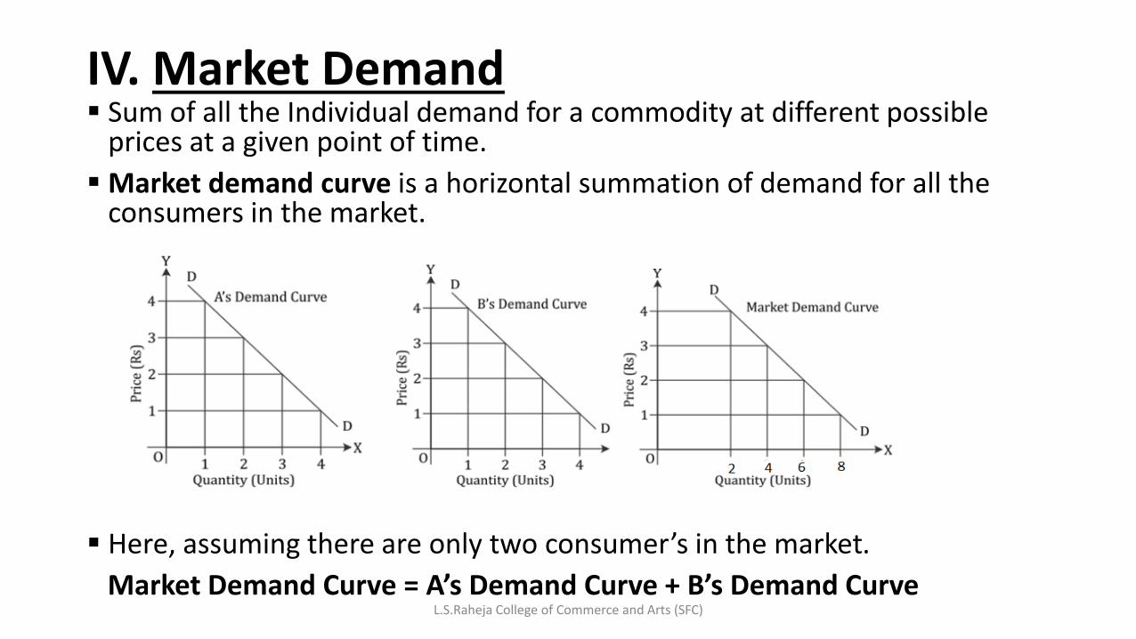
IV. Market Demand

L.S.Raheja College of Commerce and Arts (SFC)

Sum of all the Individual demand for a commodity at different possible prices at a given point of time.

Market demand curve is a horizontal summation of demand for all the consumers in the market.

Here, assuming there are only two consumer’s in the market.

Market Demand Curve = A’s Demand Curve + B’s Demand Curve

V. Demand Function Shows the functional relationship between the demand for a commodity or service and its

determinants

VI. Determinants of demandi. Price (Px)

ii. Income (Y)

iii. Price of Related Products (Py & Pz)

iv. Taste and Preferences (T)

v. Size and distribution of Population (N)

vi. Consumer’s Expectation (E)

vii. Advertisement Expenditure ( A)

viii. Cost of Credit / Availability of Credit Facility (C)

ix. Government Policies (G)

x. Weather Conditions (W)

Demand Function—Dx = f(Px, Y, Py, Pz, T, N, E, A, C, G, W)

Linear demand function—Dx = a - bPx + cY –dPy + D Pz + eT +fN +g E + hA + gC - h G (Taxes) + iW

L.S.Raheja College of Commerce and Arts (SFC)

VIII. Classification of Demand

• Direct Demand and Derived Demand

• Short-run demand and long run demand

• Individual demand and market demand

• Joint demand and Composite demand

• Company Demand and Industry Demand

• Demand for durable goods and demand for Non-durable goods

IX. Changes in Demand

• Movement along the curve—Increase and decrease in Demand

• Shift of the Curve—Expansion and Contraction in Demand

X. Exceptions to the Law of Demand

• Giffen goods

• Snob goods

• Price Expectations

• Emergencies

• Fashion/ Illustration effect

• Habit

L.S.Raheja College of Commerce and Arts (SFC)

XI. Price, Income and Substitution Effects• Income Effect—

• Substitution Effect—

• Price Effect—

Nature of Goods Income Effect Substitution Effect Price Effect

Normal Goods Positive Positive Positive

Inferior Negative (weak) Positive (strong) Positive

Giffen Negative (strong) Positive (weak) Negative

B. SUPPLY ANALYSIS

I. Meaning—Supply refers to various quantities of a commodity which a producer will offer for sale at a particular time at various corresponding prices.

II. Law of Supply—According to the Law of Supply, there is a direct functional relationship between the quantity supplied of a commodity and its price, other things remaining constant.

Supply Function for price can be expressed as—Qsx = f (Px)

III. Individual Supply Curve and Schedule

Individual Supply Curve Supply Schedule

Price (₹ ) Quantity Supplied

1 20

2 30

3 40

4 50

5 60

The Individual supply curve and supply schedule shows direct relationship between price and quantity demanded.

The Supply Curve slopes upwards

11L.S.Raheja College of Arts and Commerce

IV. Factors Influencing Supply

• Price of the product

• Natural conditions—Weather conditions

• Technological advancement

• Availability of factors of production and their prices

• Improvement in transport

• Market structure

• Government policy

V. Exceptions to the Law of Supply

• Labour Supply

• Savings: Supply of Capital

• Exception of a Change in Price in the Intermediate Future

• Immediate Need for Cash

• Rare Collections

• Closure of Business

VI. Changes in Supply Curve

• Movement along the curve—Increase and decrease in Supply

• Shift of the Curve—Expansion and Contraction in Supply

C. Market Equilibrium

Market equilibrium (e) is attainedwhen quantity demanded(Qd) isequal to quantity supplied(Qs).

At e, Qd = Qs = Q

Pe is the equilibrium price.

Any price above Pe, say P1→ Excesssupply (D < S), Surplus

Any price above Pe, say P2→ Excessdemand (D < S), Shortage.

15L.S.Raheja College of Arts and Commerce

Chapter 3: Demand FunctionI. Nature of Demand Curve Under Different Market

Oligopoly

K

Type Price Elastic Shape

1. Perfect Competition

Perfectly elastic, ep = ∞

horizontal demand curve

2. MonopolisticCompetition

Highly elastic, ep > 1

Flatter demand curve

3. Monopoly Less elastic, ep < 1

Steeper demand curve

4. Oligopoly Segment AK: more elasticep > 1Segment KB:Inelasticep < 1

Kinked demand curve

A

B

16L.S.Raheja College of Arts and Commerce