166
Demand-driven, Concurrent Discrete Event Simulation Cohn Smart Doctor of Philosophy University of Edinburgh 2001 C.
Demand-driven, Concurrent Discrete Event Simulation
Cohn Smart
Doctor of Philosophy University of Edinburgh
2001
C.

To Catherine Smart, without whom this thesis would never have been started,
and to David L. Lyle, without whom it would never have been completed.

Abstract
The simulation of complex systems can consume vast amounts of computing
power. In common with other disciplines faced with complex systems, simulation-
ists have approached the management of complexity from two angles: sub-system
evaluation and level of abstraction. Sub-system evaluation attempts to determine
the global behaviour by determining the local behaviour and then joining these
behaviours together. Altering the level of abstraction tries to reduce the detail in
the system in areas which are less critical to the model.
Data-driven evaluation, where the computation is sparked by the arrival of
sufficient data, has been widely used as a basis for discrete event simulation.
Demand-driven evaluation uses a different impetus for computation. It actively
demands that data be sent in order for it to complete the processing. The demands
that each processing unit issues, in turn, cause other processing units to become
active. The repeated demand for finer and finer sub-solutions will eventually be
satisfied which results, in turn, with the solution of the original demand. Demand-
driven evaluation provides a coherent approach to the problem of simulating large
systems at different levels of abstraction, at a cost comparable to data-driven
evaluation. A model for both data- and demand-driven evaluation is described
which captures the total communication and computation load for each node in
the system.
I\lodels are provided for the upper-bound of processor and communication
usage. The runtime dynamics of data and demand-driven systems are investigated
with particular emphasis on the relation between the costs of generating and
transmitting an event.
Demand-driven discrete event simulation, using time intervals, is able to pro-
vide a platform with dynamic communication between the nodes, local control
of processing, efficiently uses processor power, and is conservative. If the struc-
ture being simulated is free from deadlock, then the simulation will be also. The

client-server approach means that the evaluation is easy to distribute over avail-
able processors. The use of a calendar and time intervals means that the system
is able to automatically identify, and exploit, both structural and temporal par-
allelism in the underlynig system.

Acknowledgements
I would like to thank my supervisors, G. Brebner and D.K. Arvind for all their
support and encouragement throughout the work.
I would also like to thank the staff at DRA Malvern for their support, com-
ments and for their sponsorship through a CASE award.
Lastly, I would like to thank the staff and students of the Computer Science
department for making my time here so interesting and stimulating.

Declaration
I declare that this thesis was composed by myself and that the work contained
therein is my own, except where explicitly stated otherwise in the text.
(Cohn Smart)
Table of Contents
List of Figures 5
Chapter 1 Introduction 8
1.1 The structure of the thesis ...................... 8
1.2 What is Simulation? ......................... 9
1.3 Types of Discrete Simulation ..................... 11
1.3.1 Time Advance .......................... 11
1.4 Classical Discrete Event Simulation ................. 13
1.4.1 Shared-memory multiprocessors ............... 14
1.5 Distributed Simulation ........................ 14
1.5.1 Conservative Mechanisms .................. 15
1.5.2 Optimistic Mechanisms .................... 22
1.5.3 Rollback and associated Annihilation Methods ........ 24
1.5.4 Memory management in Optimistic Systems ........ 28
1.5.5 Global Virtual Time (GVT) Computation .......... 29
1.5.6 Time Buckets ......................... 31
1.5.7 Hybrid Mechanisms ...................... 32
1.5.8 Summary of optimistic methods ............... 35
1.6 A desirable simulation system .................... 36
1.7 Problem to be addressed in this thesis ............... 37
Chapter 2 Background 39
2.1 An Approach to the Obtaining the Desirable Features .......39
2.2 Distributing data ...........................40
2.2.1 Data distribution .......................41
1
2.2.2 Data production 41
2.2.3 A potential solution ...................... 43
2.3 Related work ............................. 43
2.3.1 Request Driven v's Demand Driven ............. 43
2.3.2 Micro level ........................... 44
2.3.3 Compiler level ......................... 45
2.3.4 Language level ........................ 46
2.3.5 Demand driven Simulation .................. 46
2.4 Speedup and Efficiency ........................ 49
2.4.1 Opportunity cost ....................... 50
2.5 Binary Decision Diagrams ...................... 51
2.5.1 Reducing the tree ....................... 51
2.5.2 Combining diagrams ..................... 54
2.6 Attributes of Decision Diagrams ................... 54
2.6.1 Automatic short circuiting .................. 54
2.6.2 Maximal request set ..................... 56
2.6.3 Reduction in false negatives ................. 56
2.7 Chapter Summary .......................... 58
Chapter 3 Demand-Driven Simulation 59
3.1 Costs and Benefits of Demand-Driven Simulation ......... 59
3.1.1 The Costs ........................... 60
3.1.2 The Benefits .......................... 63
3.2 Strictness and Threshold Functions ................. 64
3.2.1 Threshold Functions ...................... 65
3.2.2 Strictness ........................... 65
3.2.3 Determining C for Threshold Functions ........... 66
3.3 Input Selection ............................ 67
3.3.1 Example ............................ 70
3.3.2 Remarks ............................ 71
3.3.3 The enumeration of all possible labelings of threshold trees 72
3.4 Modes of operation .......................... 73
2

3.4.1 Input modes 73
3.4.2 Output modes .........................75
3.5 Chapter Summary ..........................76
Chapter 4 Performance Models 77
4.1 The Conservative ELSA System ................... 77
4.2 The CMB System ........................... 81
4.3 Demand-Driven Simulation ...................... 83
4.4 Interval Manipulation ......................... 84
4.4.1 Definition and relations .................... 86
4.4.2 ELSA nodes .......................... 86
4.5 Analytical Models ........................... 88
4.5.1 The Rules of Probability ................... 88
4.6 ELSA Model .............................. 89
4.7 CMB model .............................. 90
4.8 Demand-Driven Model ........................ 91
4.8.1 Communication costs ..................... 92
4.8.2 Computation costs ...................... 94
4.9 Worked Example ........................... 95
4.9.1 Summary of notation used .................. 95
4.9.2 ELSA data-driven model ................... 96
4.10 Verification of the Models ...................... 98
4.10.1 The effect of non-independent streams ........... 99
4.10.2 Suggested improvements to the model ............ 101
4.11 Tree Network Generation ........................ 102
4.11.1 Analysis of the Distribution of the Trees Generated . . 102
4.12 Results ................................. 105
4.12.1 Graphs ............................. 106
4.13 Chapter Summary .......................... 107
Chapter 5 Experimental Results 111
5.1 The Test-bed .............................111
3
5.1.1 The Micro Model 112
5.1.2 The Macro Model ....................... 114
5.1.3 Test-bed Input/Output .................... 114
5.1.4 Model Output ......................... 115
5.2 Increasing confidence in the veracity of the simulator ....... 115
5.2.1 The gentle art of Ping-Pong ................. 116
5.2.2 Time taken to handle Data and Demand messages ..... 118
5.2.3 A comparison of the real and simulated systems ...... 119
5.3 The Measures ............................. 120
5.4 The Circuits .............................. 121
5.4.1 Binary Tree .......................... 1 22
5.4.2 Adder ............................. 1 2 5
5.4.3 The ISCAS85 Circuits .................... 133
5.4.4 Linear Shift Register ..................... 134
5.4.5 Causes of Fragmentation ................... 140
5.4.6 Example of fragmentation .................. 140
5.5 Conclusions .............................. 141
5.6 Chapter summary ........................... 142
Chapter 6 Summary and Conclusions 144
6.1 Summary of thesis ...........................144
6.2 Further work ............................. 146
6.2.1 The function/cache dichotomy ................146
6.2.2 Hierarchical evaluation ....................146
6.2.3 Managing load in a peer-to-peer network ..........147
6.3 Conclusion ............................... 147
Bibliography 151
4
List of Figures
1.1 Deadlock and Memory overflow. The number beneath each channel
denotes the time-stamp of the earliest unprocessed message (the
channel clock) . . . . . . . . . . . . . . . . . . . . . . . . . . . . . 17
1.2 Motivation for Carrier-Null Message Protocol ...........19
2.1 Publisher - subscriber communications with a single publisher 42
2.2 Decision tree for f(A, B, C) = ABC V AC ............. 52
2.3 Fully reduced decision tree for f(A, B, C) = ABC V AC ...... 53
2.4 Decision diagram for f(A, B, C) = ABC V AC ........... 53
2.5 A decision diagram for a three input AND gate . . . . . . . . . . . 55
2.6 Gate level implementation of a 2-1 multiplexor ...........56
2.7 Decision diagram for 2-1 multiplexor using a three valued logic 57
3.1 A minimum expected cost evaluation graph by the method of
Dunne and Leng ............................71
3.2 Minimum expected cost evaluation graph ..............73
4.1 A node in the ELSA system with S = 2................79
4.2 A node in the Chandy-Misra-Bryant (CMB) system with S = 2 82
4.3 A node in the demand-driven system with S = 2...........85
4.4 Venn diagram of A or B but not both ................91
4.5 A sample node . . . . . . . . . . . . . . . . . . . . . . . . . . . . . 92
4.6 A simple acyclic directed graph ...................95
4.7 Percentage error when comparing ELSA model to actual results
from DRA simulator . . . . . . . . . . . . . . . . . . . . . . . . . . 99
5

4.8 Comparison of calculated and observed communications for 74LS283
adder . . . . . . . . . . . . . . . . . . . . . . . . . . . . . . . . . . 1 00
4.9 Algorithm to generate random binary trees ............. 102
4.10 A decomposition of 11,7 ........................ 104
4.11 A comparison of data and demand-driven communication load for
a 15 node balanced binary tree . . . . . . . . . . . . . . . . . . . . 105
4.12 Effect of granularity on work done .................. 107
4.13 Effect of granularity on communication performed ......... 108
4.14 Effect of increasing the frequency of events on work done ..... 108
4.15 Effect of increasing the frequency of events on communication . 109
4.16 Effect of strictness on work done ................... 109
4.17 Effect of strictness on communication performed .......... 110
5.1 The time taken for a two way message on Calvay ......... 117
5.2 The time taken for a two way message on Balta .......... 117
5.3 The time taken for a two way message on a pair of SS5 machines 118
5.4 Samples of the time taken to handle a data or demand message 120
5.5 Runtimes of both the real and test-bed simulators ......... 121
5.6 The 256 node binary tree used in the following experiments . . . 123
5.7 Tree 256: Data-driven runtime as a function of Tsend and Tdata
for a 9-processor machine ....................... 124
5.8 Tree 256: Demand-driven runtime as a function of Tsend and Tdata
for a 9-processor machine ....................... 124
5.9 Completion time as a function of the number of processors (Note:
the x axis is logarithmic) ....................... 125
5.10 Speedup evident in a 256-node tree for both data- and demand-
driven simulation . . . . . . . . . . . . . . . . . . . . . . . . . . . . 126
5.11 Efficiency evident in a 256-node tree for both data- and demand-
driven simulation . . . . . . . . . . . . . . . . . . . . . . . . . . . . 127
5.12 Tree 256: Graphs of Completion time and Work performed for
differing values of Tsend and Tdata ................. 128
5.13 Tree 256: Graphs of Completion time and Work performed for
differing values of Tsend and Tdata (cont.) ............. 129
5.14 Topological layout of the 74LS283 adder .............. 130
5.15 Adder: Data-driven runtime as a function of Tsend and Tdata for
a 9-processor machine ........................ 131
5.16 Adder: Demand-driven runtime as a function of Tsend and Tdata
for a 9-processor machine ... . . . . . . . . . . . . . . . . . . . . . 131
5.17 Adder: Graphs of Completion time and Work performed for dif-
fering values of Tsend and Tdata .................. 132
5.18 Adder: Graphs of Completion time and Work performed for dif-
fering values of Tsend and Tdata .................. 132
5.19 C880: Data-driven runtime as a function of Tsend and Tdata for a
9-processor machine .......................... 134
5.20 C880: Demand-driven runtime as a function of Tsend and Tdata
for a 9-processor machine ....................... 135
5.21 C880: Graphs of Completion time and Work performed for differ-
ing values of Tsend and Tdata .................... 136
5.22 C880: Graphs of Completion time and Work performed for differ-
ing values of Tsend and Tdata .................... 137
5.23 ..................................... 138
5.24 LFSR Base Unit ............................ 139
5.25 Hierarchical Composition of Benchmark .............. 139
7
Chapter 1
Introduction
The problem of efficiently executing regular, parallel programs has been much
studied, and machines such as the Connection Machine[41] were designed to fa-
cilitate such computation. Such early parallel machines were designed for parallel
computation from the outset. Recently there has been a change of focus, away
from monolithic systems, towards utilising a networks of workstations where the
parallelism is supported more by the operating system and less by dedicated
hardware. Examples of such systems are the SETI©Home[50] and Beowulf[861
projects.
The area of irregular computations, however, has been less extensively exam-
ined. Irregular computations are characterised by an execution pattern which
cannot be predicted in advance and which is very sensitive to the input data.
Parallel discrete event simulation is one such irregular computation and is used
throughout to illustrate the methods employed.
1.1 The structure of the thesis
Chapter 1: Introduction. This chapter introduces distributed discrete-event
simulation as a means to explore irregular computation and, after a review
of the major approaches to time synchronisation in such systems, proposes a
new method that addresses an aspect of efficiency which has been overlooked
by the other approaches.
Chapter 2: Background. This chapter steps back from simulation and looks
at the more generic problems of the production and synchronisation of data
in distributed systems, and how it relates to the desirable features of a
dynamic communications topology, freedom from deadlock, local control
and efficient use of resources.
Chapter 3: Demand-driven Simulation. This chapter discusses some of the
costs and benefits associated with demand-driven simulation. The costs
are resource consumption, be they bandwidth, processor or time. It pro-
vides arguments in mitigation of a number of the costs involved as well as
strategies to reduce the overall cost of simulating a system.
Chapter 4: Performance models. This chapter first describes, in detail, the
behaviour of Chandry-Misra-Bryant, ELSA and demand-driven systems. Af-
ter providing background definitions, models are derived which express the
upper-bound of the gross computation and communication behaviour of
those systems.
Chapter 5: Experimental results. This chapter uses a number of different
circuits to examine the dynamic nature of the simulation and, in particu-
lar, to focus on the parallelism and performance which is available as the
computing resource increases.
Chapter 6: Summary and Conclusions. This chapter summarises our work,
provides some discussion of our conclusions and gives some directions for
further work in the area of demand-driven systems.
1.2 What is Simulation?
Computer simulation involves the construction of a mathematical model of a
system in which mathematical symbols and equations are used to represent the
relationships between objects in the system. The calculations indicated by the
model's equations are then performed repeatedly, using a computer with time
incremented discretely, to represent the passage of real-world time. The computer
simulation indicates the behaviour of the mathematical model and from this is
inferred the behaviour of the modelled system.
09

Computer simulation is currently used in a wide range of applications, espe-
cially in engineering and the physical sciences, where systems are expensive or
difficult to analyse. Much of what is known about many safety critical applica-
tions is derived from computer simulation; for example, if testing of the real world
system under extreme conditions would involve excessive risks, then simulation
must be used to determine the system's likely behaviour. Similarly, the likely
performance of a new system is often assessed from simulation studies. This is
particularly so when, for safety reasons, a system cannot be allowed to 'go live'
in an untested configuration, or when it is impractical to experiment with the
environment with which the system interacts.
Clearly, the integrity of the computer simulation is of critical importance; the
simulation must be designed with care, so that the results obtained are valid,
accurate and useful.
Most systems may be defined as a collection of elements which inherently
execute concurrently and interact one with another to achieve some global func-
tion. For example, the human heart, lungs and bloodstream form a physiological
system whose purpose is to provide oxygen for the body; each component ex-
ists and operates largely autonomously, yet the overall function is achieved by
the interaction of the components. By analogy, any model should include what-
ever concurrency and inter-process interactions exist in the real-world system,
and the simulation should be able to handle that concurrency and inter-process
interaction.
The ready availability of low-cost parallel processing elements makes it in-
creasingly attractive to use true parallel processing and true process interaction
in simulation. A number of specific problem domains have been explored and a
variety of systems have been reported (a few of these systems are examined in
detail below). These reports have shown that complex systems can be modelled
easily and economically, keeping a close relationship between the model and the
real-world system, and without compromising the natural concurrent nature of
the real-world system. In addition, the use of parallel computers can lead to
substantial performance gains.
10
There are two classes of model available: continuous and discrete. A contin-
uous model is used where the system varies continually with time. A discrete
simulation is used when we are more concerned with the transitions from state
to state than with the times at which they occur. We shall look only at discrete
models.
1.3 Types of Discrete Simulation
An event is an action which can occur within the system being simulated.
In a discrete simulation the state of the system is assumed to remain constant
between events. By making the interval between events smaller and smaller, an
approximation of a continuous system can be achieved, though there will always
be inaccuracies.
1.3.1 Time Advance
The method for advancing time in a discrete simulation system can be used to
partition the methods into two classes:
• Time-driven simulation. This method is also known as compiled mode sim-
ulation. In this system, the continuous flow of time is modelled as a suc-
cession of equally spaced steps. The entire system is evaluated for each of
those steps. A disadvantage of this method is the inherent assumption that
the state of the system at time t + R can be determined by some function of
the state at time t and the inputs to the system at time t+6t. This method
also fails to record changes to the system in the interval (t, t + öt). It does,
however, have the advantage that no scheduling is necessary (as the whole
system is evaluated every St). Also, it is relatively simple to implement
on parallel or distributed machines as there is no synchronisation required
between the components of the system to impede the execution.
• Event driven simulation. If we consider the system to be simulated as a
number of elements, each of which maintains a local state which, in turn,
is used as the input state to a number of other elements, then an event
11
driven simulation can be employed. The number of elements whose inputs
change at any given time is generally quite small and much of the execution
time in a time driven simulation is wasted, either recalculating an output
whose inputs have not changed, or in checking to see what has changed. An
alternative approach is to mark each change in state with the time at which
that change takes effect. The simulator thus knows what, and when, states
change. For some systems, the overhead in maintaining this extra state
information makes the event driven system perform poorly compared with
time-driven systems although it can perform better if the state changes are
rare (either in time or space).
A timing model is used to mimic the time taken by a element to determine the
new output value when one or more input values change. A number of different
timing models are available.
• Unit delay assumes that every change of an input state requires exactly one
time unit before its effect appears as an output state. It is worth noting
that a change in the input state does imply a change in the output state.
This is the only timing model available to time-driven simulation.
• Fixed delay assigns individual delays to each element and keeps these delays
constant throughout the entire simulation. This can be used to mimic the
granularity (or response time) of the element in question. Should the time
taken to process a change in state depend on the specific transition being
experienced by the element (from old input state to new input state) then
multiple fixed delays can be applied.
• Variable delay provides a more flexible way to simulate elements. With
this type, the value of the delay changes to reflect the state of the system.
For example, a car waiting to cross a train track will have a delay which
varies with the speed and length of the train; values which may be data
dependent.
12
1.4 Classical Discrete Event Simulation
In a classical discrete event simulation system, a queue holds an ordered list of
event-time pairs. The list is ordered on the time component of the pair. In effect,
the pair dictates what happens and when it happens.
Each event can cause a number of other events, including itself, to be scheduled
in the future. Some systems permit events to be scheduled at the current time,
while others expressly forbid such scheduling in order to ensure the progress of
time. No event can cause an event to be scheduled in the past. A simulation
system, then, consists, in the abstract, of a single queue which holds the scheduled
events in time order. Events with the same time-stamp are evaluated in an order
determined by a resolution strategy. This strategy can be as simple as first-
come first-served. In some models, the existence of two conflicting events, such
as "increase heat" and "decrease heat", scheduled for the same time is an error
condition which halts the simulation.
The simulation proceeds by executing the event at the front of the queue (the
event with the lowest time-stamp) and inserting into the queue any resulting
events. This continues until either a preset time or condition is reached, or the
queue becomes empty.
Early attempts at parallelising the simulation were still based on the single
queue model of the sequential methodi271. It was thought that, as there could be
a number of events in the queues with the same time-stamp, a performance gain
could be achieved by executing all such events on separate processors. While this
did improve performance, such systems had a number of drawbacks, the most
notable being that the single queue proved to be a bottleneck in the system.
While one processor was executing the last of the events with the current time-
stamp, the rest of the system had to wait until it had finished before issuing events
with a higher time-stamp. If one event scheduled another event with the same
time-stamp, then the system had to process these sequentially, with the resultant
loss of parallel performance.
This was confirmed by Agrawal[2] and others. Work then began on a num-
ber of more complex queuing models which eventually resulted in the Chandy-
13
Misra[19] or Bryant[13] systems, which will be described in Section 1.5.
1.4.1 Shared-memory multiprocessors
There have been many attempts to apply parallel computers to discrete-event
simulation. These may be divided into two main approaches, distributed sim-
ulation and concurrent simulation. Distributed simulation relies on a spatial
decomposition and partitions the simulation model into components that can be
executed on different processors. Concurrent simulation is based on a temporal
decomposition.
While this thesis concentrates on distributed simulation, some developments in
shared-memory concurrent simulation[23, 90] are worthy of mention. Many of the
performance-degrading obstacles found in distributed memory simulations, such
as communication delay, null messages, and the high cost of deadlock detection
and recovery, can be reduced. Near ideal speed-up for several queuing network
simulation models using shared-memory distributed simulation has been reported
by Wagner and Lazowska[90, 91].
Hoeger and Jones[42] have integrated the two distributed and concurrent ap-
proaches. They have produced a distributed simulator with concurrency added
to each model component. This was done in a shared-memory environment and
:both approaches were unified to an event-centered view. They partitioned the
global event queue of the concurrent simulator and provided each model com-
ponent in the distributed simulator with a local concurrent event queue which
allowed them to add concurrency to each model component.
1.5 Distributed Simulation
The field of distributed simulation has received a great deal of interest and nu-
merous methods have been developed to maintain a sufficiently accurate view of
time across a collection of processing elements. In this section we shall start by
providing a brief overview of distributed simulation and then follow with a survey
of the different approaches that have been taken to address the issues raised by
successive systems.
14
In distributed simulation, the physical system is usually modelled as a set
of spatially separated physical processes that interact at discrete time instants.
The distributed simulation approach maps each physical process onto a logical
process (LP) of the simulation engine. Interaction between physical processes is
handled via time-stamped messages, exchanged between the corresponding logi-
cal processes. Each LP maintains its own local clock - often referred to as Local
Virtual Time (LVT) - and a local event queue holding messages in time order.
A synchronisation protocol has to be provided and executed by each logical pro-
cess in order to preserve the dependency between events in this asynchronous
environment. In the simulation engine, the logical processes are mapped to pro-
cessors; the communication links are embedded in the underlying inter-processor
communication network. This provides a natural means, not only for exploiting
parallelism, but also for maintaining the modularity of the simulation.
Two different styles of synchronisation have, until recently, further divided
distributed simulation into two classes; conservative and optimistic.
1.5.1 Conservative Mechanisms
The essential basis of distributed simulation was first presented by Chandy and
Misra[19], and independently by Bryant[13. Such systems are sometimes referred
to as CMB (Chandy, Misra, Bryant) systems.
In CMB systems, the causality of events across all the LPs is preserved by
sending time-stamped event messages (<event©t>); the time-stamp is a copy of
the LVT of the sending LP. A conservative logical process is allowed to process
safe events only. A safe event is one which has a time-stamp in advance of the
LVT of the receiving LP, but less than (or equal) to the time-stamps on all other
messages which the LP will receive. All events must be processed in chronological
order. This guarantees that the output stream of a LP is in chronological order.
A communication system preserving the order of messages sent from one LP to
another (FIFO) is sufficient to ensure that no out of chronological order messages
will ever arrive at receiving LP. A conservative system can thus be seen as a set
of all LPs together with a set of directed, reliable, FIFO communication channels
15
that constitute a graph of logical processes. It is important to note that this
graph has a static topology.
The communication interface of a logical process maintains an input buffer
and a clock for each channel pointing to that LP. The buffer stores every message
arriving through a channel in FIFO order and that channel's clock is set to the
time-stamp of the earliest unprocessed message (the one at the head of that
channel's buffer). Initially the value of every channel clock is set to zero.
The local virtual time is the minimum of the channel clocks. This gives the
time horizon, up to which it is safe to process events. It is safe because, given
the FIFO links and a fixed topology, it is not possible for any LP in the system
to send a message down a channel with a time-stamp less than already sent and
no LP can send a message without having started at a LVT of 0.
The event (or events) with a time-stamp equal to the LVT are processed and
removed from the input buffer and any resultant events dispatched. Given that
there are now no messages left with a time-stamp equal to LVT the LP can
perform one of two actions. If there is a message on all of the input arcs then the
LP can increase its LVT to the new minimum and repeat, or it must wait until
all the channels have messages before repeating. This "blocking until safe" policy
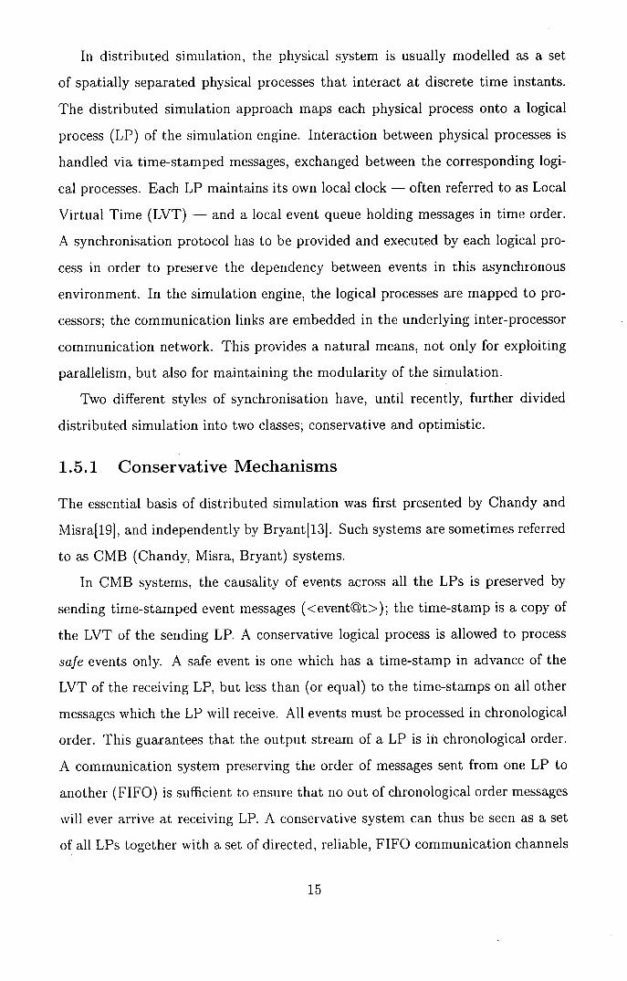
leads to two problems: deadlock and memory overflow as shown in Figure 1.1.
Each LP is waiting for a message to arrive from a LP which is itself blocked
(deadlock). Also, each process which is blocked is receiving messages from non-
blocked LP which are being queued and left unprocessed in their respective input
buffers. These input buffers can grow unpredictably and thus cause memory
overflow. This is possible even in the absence of deadlock. Several methods have
been proposed to overcome the vulnerability of CMB to deadlock, these fall into
two principal categories: deadlock avoidance and deadlock detection/recovery.
1.5.1.1 Deadlock Avoidance
Deadlock, such as that in Figure 1.1, can be prevented by modifying the com-
munication protocol so that null messages[60 (messages of the form <null@t>,
where null is an event with no effect) can be sent. A null message is not related
16
to the simulated model and serves only as a synchronisation method. It is sent
on every output channel as a statement that that LP has reached a certain value
of LVT and thus will never send out a message with a time-stamp less than t. A
null message is sent to every target LP for which the sending LP did not generate
any other message. The effect is to notify every target LP of the sending LP's
new LVT. The receiving LP can use this information to increase the channel clock
on the corresponding link and thus permit other events to be processed.
iIII_
29
iIII
IIIIL
'
2
iIIII
19 88
14
IIII
iI--
4
*
3
L2' 19
II
LVT
Figure 1.1: Deadlock and Memory overflow. The number beneath each channel denotes the time-stamp of the earliest unprocessed message (the channel clock).
In Figure 1.1, after the LP in the middle had sent <nu1l19> to the neigh-
bouring LPs, both of them could increase their LVT to 19 and in turn issue new
event messages to other LPs. The null message protocol can be guaranteed to
be deadlock free as long as there are no closed cycles of channels, for which a
message traversing this cycle cannot increase its time-stamp. This implies that
simulation models cannot be simulated using CMB with null messages, if they
cannot be decomposed into LP such that for every directed channel cycle there
is at least one LP to put a non-zero time increment on traversing messages.
Although the protocol is straightforward to implement, it can put a greatly
increased burden on the communication network (as a result of the null messages)
and also reduce the performance of the simulation, as each null message needs
to be processed. Optimisations on the protocol to reduce the frequency, or num-
ber, of null messages have been proposed[60. An approach whereby additional
information is carried with the null message (the so-called carrier-null message
17
protocol[17]) will be looked at in Section 1.5.1.2.
One remaining problem with trying to improve the performance of conser-
vative logical processes is determining when it is safe to process an event. The
degree to which LPs can look ahead and predict future events can play a critical
role in the safety verification, and thus the performance, of conservative LP sim-
ulations. In Figure 1.1, if the LP with LVT of 19 knew that processing the next
event will increment the LVT to 22 then it could send a null message <null©22>
(a look-ahead of 3) to improve the LVT of the receivers.
Look-ahead must come directly from the underlying simulation model and
enhances the prediction of future events; the ability to exploit look-ahead was
first shown by Nicol[66] for FCFS queuing network simulations.
1.5.1.2 Carrier-Null Message Protocol
As mentioned in the previous section, it is possible to augment the null message
with other information to help overcome some of the inefficiencies of the null
message protocol. Consider the system shown in Figure 1.2. The source creates
an event every 50 virtual time units; the join, split and pass units each take 2
virtual time units to handle the event. After the first event is released by the
source, all LP except the source are blocked and start to propagate local look-
ahead via null messages. After 4 null messages (join to pass, pass to split, split
to join and split to sink) each of those LP has advanced their local time by 2
virtual time units. It will take a further 96 null messages (100 in all) before the
initial source event can be processed and then another 100 null messages before
the second source event can be processed, and so on. The impact of look-ahead
is easily seen in this example; the smaller the look-ahead on the successor LPs,
then the more null messages that will have to be sent to advance the virtual time,
resulting in a higher communication load and thus a poorer performance. In a
study by Leung and others[51] it was shown that cycles in the communication
network of a conservative CMB system can remove almost all the speedup from
the system.
The carrier-null message protocol[171 aims to reduce the number of null mes-
T]
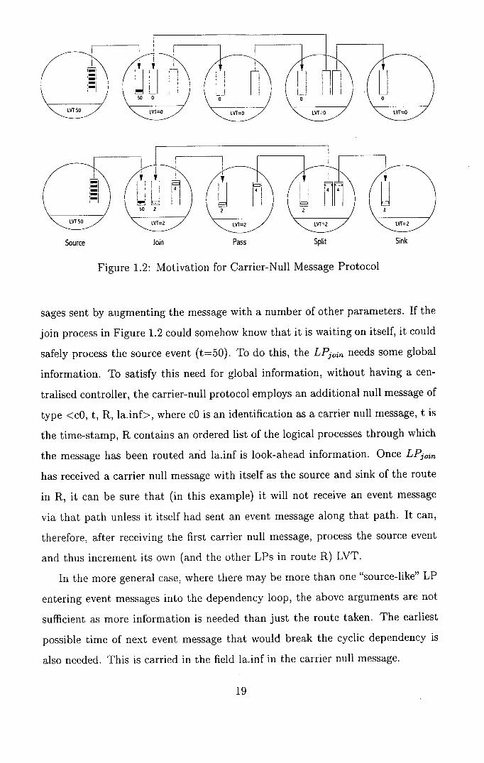
• 'rM,n KJ K L) t-Y1=o
Source Join Pass Split Sink
Figure 1.2: Motivation for Carrier-Null Message Protocol
sages sent by augmenting the message with a number of other parameters. If the
join process in Figure 1.2 could somehow know that it is waiting on itself, it could
safely process the source event (t=50). To do this, the LPj,i,, needs some global
information. To satisfy this need for global information, without having a cen-
tralised controller, the carrier-null protocol employs an additional null message of
type <cO, t, R, la.inf>, where cO is an identification as a carrier null message, t is
the time-stamp, R contains an ordered list of the logical processes through which
the message has been routed and la.inf is look-ahead information. Once LP30
has received a carrier null message with itself as the source and sink of the route
in R, it can be sure that (in this example) it will not receive an event message
via that path unless it itself had sent an event message along that path. It can,
therefore, after receiving the first carrier null message, process the source event
and thus increment its own (and the other LPs in route R) LVT.
In the more general case, where there may be more than one "source-like" LP
entering event messages into the dependency loop, the above arguments are not
sufficient as more information is needed than just the route taken. The earliest
possible time of next event message that would break the cyclic dependency is
also needed. This is carried in the field la.inf in the carrier null message.
19
Even with carrier null messages, the CMB system can still produce many
null messages. An approach by Preiss and others[72] attempts to reduce null
message propagation by recognising when a null message has become superseded
(or stale). Suppose that a LP has sent a stream of null messages to another LP.
For example, this might occur when the originating LP has more than one input
channel. Each of these null messages will have an increased time-stamp. The
null messages will be queued at the input buffer until being processed. Should a
null message with time-stamp t arrive in the buffer and find another null message
with a time-stamp s < t then there is no point having the receiving LP process
the earlier null message as it it now redundant and can be annihilated. This was
generalised further to say that any message from the same source which finds a
null message with a smaller time-stamp may annihilate that null message. This
optimisation depends on the respective rate of production and consumption of
null messages and may, in the case where the LP is a greedy consumer, produce
no performance improvement whatsoever.
A later study, by Teo and Tay1881, of the conservative simulation of a multi-
stage interconnection network uses a similar "flushing" method to that proposed
by Preiss[721. In the example used by Teo and Tay, the amount of null message
overhead was reduced from exponential to linear in the number of elements in the
system. This has important repercussions on the performance of the system as
Soule[821 notes that, in parallel event-driven simulation of logic circuits, 50% to
80% of the execution time is spent in the deadlock detection and recovery phases.
1.5.1.3 Deadlock detection and recovery
An alternative to the null message approach was also proposed by Chandy and
MisraI19j, which allowed deadlocks to occur but provided a method to detect
them and recover. Their algorithm has two phases: the first (a parallel phase), in
which the simulation runs until it deadlocks, and the second (an interface phase),
that starts a computation which results in at least one LP being able to advance
its LVT. They prove that, in every parallel phase, at least one event will be
processed, generating at least one event message which will also be propagated
20
before the next deadlock. Their algorithm assumes a central controller, which
violates a central tenet of distributed computing. This was later removed and
replaced with a distributed deadlock detection algorithm[20].
Misra[601 proposes an alternative approach in which a special message (called a
marker) circulates through the network of channels to detect and resolve deadlock.
A cyclic path for traversing all the channels is precomputed and all LPs are
initially coloured white. A LP that receives the marker turns white and forwards
it along the path in finite time. Once a LP has forwarded the marker, should it
either send or receive an event, then it turns red. Deadlock is detected by the
marker if the last N LP visited were all white. If the marker also carries the next
event times of the visited (white) LPs then it will know, once it has detected
deadlock, the smallest next event time as well as the LP in which this is supposed
to occur. To recover from deadlock, this LP is invoked to process its earliest
event.
The time-of-next-event algorithm proposed by Groselj and Tropper[381 as-
sumes more than one LP mapped to a single physical processor and computes the
lower bound of the time-stamps of the event messages expected to arrive next at
all empty links on the LPs located at the processor. It thus helps to unblock LPs
within one processor but does nothing to prevent deadlocks across processors.
An optimisation has been adopted by Soule and Gupta[83]. Their work is
specific to logic simulation and centres on manipulating the order in which nodes
are evaluated to reduce the potential for deadlock. In some cases, all deadlock
has been removed.
1.5.1.4 Summary of conservative methods
The principle of conservative operation is that causality violations are strictly
avoided; only "safe" events are processed. The synchronisation method is pro-
cess blocking, which can cause deadlock. This is inherent in the protocol and
not a resource contention problem. Deadlock prevention protocols based on null
messages are liable to place a severe communication overhead on the system.
Deadlock detection and prevention algorithms mainly depend on a centralised
21
controller, though other methods are available. The parallelism available within
a CMB system is purely structural and rarely fully exploited as, if causality vi-
olations are possible, even if rare, the protocol behaves overly pessimistically as
it waits until it is not possible for a violation to occur. CMB performs well as
long as all channels are equally utilised. Should a channel not have a new event
message, because the state has not changed, then either it will need to send null
messages or become involved in a deadlock detection and recovery process. A
large dispersion of events in either space or time does not degrade performance.
This is because a conservative LP is only concerned with the earliest message
from those LPs that are directly connected to it. The potential zone of influence
of a LP is small and thus it is relatively insulated from the rest of the simulation
system.
There is no explicit computation of a global virtual time (GVT) which, as we
will see in Section 1.5.5, is needed to manage memory in optimistic systems. The
global virtual time is the time before which no events can occur.
A conservative system can cope with simulation models having "arbitrarily"
large state spaces and is straightforward to implement using only simple control
and data structures, though it does require that the communication channels are
FIFO and that events are processed in the order of their arrival (which will be, un-
der the strictures of the protocol, in chronological order). The LP interconnection
topology must be static.
While no general performance statement is possible owing to the many dif-
ferent systems, implementations and architectures, the performance of a CMB
system relies mainly on its deadlock management strategy. The computation and
communication overhead per event is small on average and the protocol favours
"fine grain" simulation models.
1.5.2 Optimistic Mechanisms
The "pessimistic" causality constraint of the conservative system strictly prevents
any out of order execution of events. In contrast, optimistic LP simulation strate-
gies allow causality errors to occur and provide a method whereby the system can
22

recover from such violations. In order to avoid the blocking and safe-to-progress
determination which hinder the performance of conservative systems, optimistic
processes evaluate events (and hence advance LVT) as far into the future as pos-
sible. This is done with no regard for causality errors and there is no guarantee
that an event will not arrive in the local past.
1.5.2.1 Time Warp
The initial work in optimistic simulation was by Jefferson and Sowizral[45, 48]
with the definition of the Time Warp (TW) mechanism which, like the Chandy -
Misra-Bryant protocol, uses messages for synchronisation. The Time Warp mech-
anism restores consistency with the local causality constraints[34] through the use
of a rollback mechanism. If an event arrives with a time-stamp in the local past,
i.e. out of chronological order (these messages are sometimes referred to as strag-
gler messages), then the TW scheme rolls back time to the most recently saved
state in the LP history which is consistent with the time-stamp on the new mes-
sage and restarts the simulation from that point.
Rollback requires a record of the history of the LP so that it can return to a
point in its past and correct the causality error. This mean a record not only of
internal state changes, but also of the contents of input and output queues. For
reasons which we will cover later, the record of the LP's communications history
must be done in chronological order.
Since the arrival of event messages in increasing time-stamp order cannot
be guaranteed, two different kinds of messages are required to implement the
communications protocol. The first is the usual CMB style message but with
an added '+' field ( m + =< ee@t, + >), where again ee is the event and t is a
copy of the sender's LVT. Subsequently we will refer to this type of message as a
Positive message. To balance positive messages, we also have negative messages
(or anti-messages) of the form (m =< ee(5t, - >). These negative messages are
transmitted to a LP to request the annihilation of the prematurely sent positive
message containing ee. This would occur when the sending LP discovered that
the value of ee was computed based on a causally erroneous state.
23

The basic architecture of an optimistic LP is similar to that for a conservative
LP. Again messages are transmitted through a communications system but they
are not required to arrive in the order that they were sent and this relaxes the
hardware requirements. Also it is not necessary to separate the input streams, so
a single input queue is sufficient (as long as the sending LP can be identified from
the message). The communication history must be stored, as must the internal
state.
An optimistic LP works in four phases: input synchronisation to other LPs,
local event processing, the propagation of external effects and the global confir-
mation of locally simulated events. The event processing, and propagation of ex-
ternal effects, are almost the same phases as those contained within a conservative
system. The input synchronisation (rollback and annihilation) and confirmation
are the key elements in an optimistic LP simulation.
1.5.3 Rollback and associated Annihilation Methods
The rollback mechanism relates the incoming message with the current state of
the LP to determine the appropriate action. There are three possible variables
to consider; the type of the arriving message (mt, mj, the relation of the time-
stamp to the LVT (time-stamp ~! LVT, time-stamp < LVT) and whether a dual
message exists (a m+ for a m or a m for a m+). The appropriate action is
outlined in Tables 1.1 and 1.2.
Arriving message is of type: m +
time-stamp > LVT if dual m exists if dual m does not exist (in the local future) annihilate dual m chronologically insert (m,IQ) time-stamp < LVT if dual m exists if dual m does not exist (in the local past) annihilate dual m rollback then
chronologically insert (m,IQ)
Table 1.1: Appropriate actions on receiving an incoming positive message in a Time Warp based protocol
Events which arrive in the local future are unproblematic as they have yet to be
processed and, as such, cannot have had an effect outwith the local environment.
So, should a positive message arrive it will either a) cancel out an existing negative
24
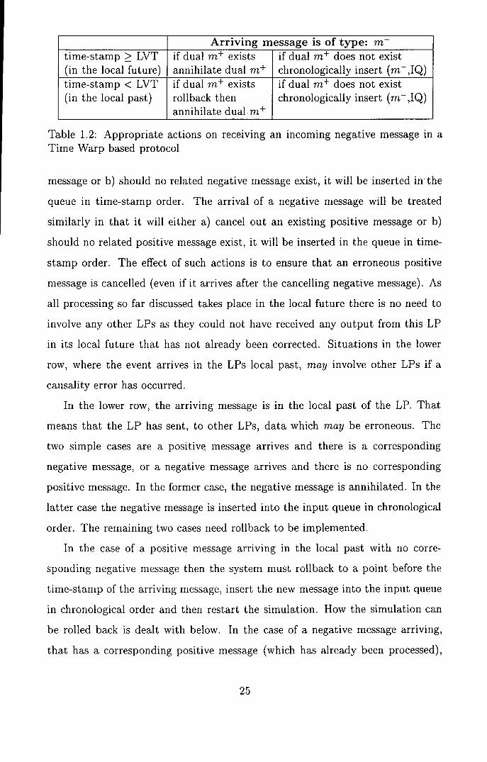
Arriving message is of type: m time-stamp > LVT if dual m exists if dual m does not exist (in the local future) annihilate dual m chronologically insert (m,IQ) time-stamp < LVT if dual m exists if dual m does not exist (in the local past) rollback then chronologically insert (m,IQ)
annihilate dual m+
Table 1.2: Appropriate actions on receiving an incoming negative message in a Time Warp based protocol
message or b) should no related negative message exist, it will be inserted in the
queue in time-stamp order. The arrival of a negative message will be treated
similarly in that it will either a) cancel out an existing positive message or b)
should no related positive message exist, it will be inserted in the queue in time-
stamp order. The effect of such actions is to ensure that an erroneous positive
message is cancelled (even if it arrives after the cancelling negative message). As
all processing so far discussed takes place in the local future there is no need to
involve any other LPs as they could not have received any output from this LP
in its local future that has not already been corrected. Situations in the lower
row, where the event arrives in the LPs local past, may involve other LPs if a
causality error has occurred.
In the lower row, the arriving message is in the local past of the LP. That
means that the LP has sent, to other LPs, data which may be erroneous. The
two simple cases are a positive, message arrives and there is a corresponding
negative message, or a negative message arrives and there is no corresponding
positive message. In the former case, the negative message is annihilated. In the
latter case the negative message is inserted into the input queue in chronological
order. The remaining two cases need rollback to be implemented.
In the case of a positive message arriving in the local past with no corre-
sponding negative message then the system must rollback to a point before the
time-stamp of the arriving message, insert the new message into the input queue
in chronological order and then restart the simulation. How the simulation can
be rolled back is dealt with below. In the case of a negative message arriving,
that has a corresponding positive message (which has already been processed),
25
the system must roll back to point before the time-stamp of the arriving message,
annihilate the associated positive message, and then restart the simulation from
that point.
As can be seen, the rollback mechanism requires a periodic saving of the state
of the LP. This allows the LP to rewind to some state before the causality error
occurred and then to continue processing past the now corrected error. It is also
necessary to maintain a log of all outgoing messages in order to undo events
which have been propagated to external LPs. Observe from the table that anti-
messages can also cause rollback and, as such, can cause rollback chains in which
one LP, in rolling back, causes other LPs to rollback. It is even possible for
recursive rollback to occur should a LP in a cycle start to rollback. The protocol
guarantees that any rollback chain will eventually terminate whatever its length
or recursive depth. Such a rollback chain can consume significant memory and
communication resources.
1.5.3.1 Aggressive Cancellation
The original Time Warp protocol described, in part, above used aggressive cancel-
lation. Using this form of cancellation whenever a straggler message (a message
with a time-stamp in the local past) arrives, anti-messages are sent immediately
to cancel all potentially incorrect messages. The aim of this was to reduce the
number of potentially erroneous messages being processed by external LPs which
may, in turn, force them to roll back.
1.5.3.2 Lazy Cancellation
A different cancellation policy was proposed by GafniI361, which he termed Lazy
cancellation. In this alternate policy, the system does not send anti-messages
immediately upon the receipt of a straggler message. Instead the system delays
the propagation until the LVT has, after rollback, reached the time-stamp on the
straggler message and the system produces a different output message from that
originally sent at that time-stamp. In this case the earlier message which was sent
has been shown to be incorrect and needs to be cancelled. If the resimulation
resulted in the same message being generated as had originally been sent then no
26
cancellation is necessary. Lazy cancellation thus avoids unnecessary cancellation
of correct messages but does have the overhead of additional memory and book-
keeping (potential anti-messages must be maintained in the output queue). It also
delays the cancellation of incorrect messages, which may result in more rollbacks
being needed downstream of the causality error.
The idea of lazy cancellation can be expanded, using the look-ahead value
(Ia) first mentioned in Section 1.5.1.1, to reduce the number of rollbacks that are
needed to maintain causality. If a straggler message ts(m+) <LVT is received
then there is no need to send anti-messages for any message with a time-stamp
less then ts(m) + Ia. Also, if ts(mj + la >LVT then rollback does not need to
be invoked.
Jefferson[47] has shown that Time Warp with lazy cancellation can outperform
the simulation's critical path. This is possible because calculations based on the
assumed state of the system, which was later confirmed to be correct, would have
propagated further through the system than they would have done under either
conservative or aggressive cancellation strategies. This has the effect getting the
correct value to the input of an element before it has been confirmed. This effect
was termed "supercritical speedup". Aggressive cancellation does not have this
potential as rolled back computations are discarded immediately. A comparison
of the performance of the two is, however, related to the simulation model. It
has been shown by Reiher et al.175] that lazy cancellation can arbitrarily out-
perform aggressive cancellation and vice versa. While their study used synthetic
extreme cases to highlight the strengths and weaknesses of each protocol, the
empirical evidence is reported "slightly" in favour of lazy simulation for certain
applications [36, 341.
Fujimoto[33] has adapted distributed simulation to the shared-memory multi-
processor environment, and also utilises shared memory to optimise the message
cancellation process. The handling of roll-back can be a major overhead in a
simulation and, as such, work has been done on providing hardware support for
this operation 131•
27
1.5.3.3 Breaking or Preventing Rollback Chains
A number of other techniques, beside lazy cancellation, have been used to limit the
number of rollbacks in a system. One approach, which was based on the carrier-
null approach discussed earlier, was proposed by Prakash and Subramanian[71].
They attached a limited amount of state information to messages to prevent
recursive rollbacks. The attached state information allowed LPs to filter out
those messages which were based on an assumed state of the system. These false
positive messages would eventually be annihilated by chasing anti-messages which
were currently in transit.
Madisetti, Wairand and Messerschmitt[56] proposed a protocol called Wolf-
calls. In this protocol, events based on the assumed state of the system, are able
to propagate to a limited set of LPs within a specified distance of the source LP.
These spheres of influence are defined as the set of LPs which can be affected
by an event in a certain time (respecting both communication and computation
times). The effect is to limit the number of LPs which can be affected and
thus limit the length of the rollback chain. Dickens and Reynolds[28] proposed a
variation on this idea with the SRADS protocol in which, while allowing optimistic
progression, the propagation of uncommitted events to external LPs is prohibited.
This means that rollback is local and that rollback chains can never occur.
1.5.4 Memory management in Optimistic Systems
The discussion so far has assumed the availability of sufficient free memory to
store internal and external history for pending rollbacks. Lin[54] argues that
Time Warp always consumes more memory than sequential simulation and that
limiting the memory imposes a performance decrease. Providing merely the
minimum amount required causes such a decrease in performance that a mem-
ory/performance tradeoff becomes an important issue.
There are two ways of limiting the amount of memory used in an optimistic
system: i) reduce the amount of optimism as occurs in the systems proposed
by Madisetti and by Dickens or, ii) save the state of the system infrequently or
incrementally. Neither system can guarantee that memory will not be exhausted
and so it is necessary for the protocol to recover memory no longer needed by the
system. This fossil collection is used to reclaim the memory being used to store
events and states which will never be needed by the system because the global
virtual time has progressed beyond their time-stamp. The global virtual time is
the minimum time-stamp on any unprocessed event in the system.
1.5.4.1 Incremental State Saving
Many models have large and complex internal states which have to be stored.
With each processed event, some of the variables which comprise the state will
change while others will remain unchanged. An improvement can be made by
only saving the variables which have changed. This "incremental state saving"
was first proposed by Bauer et al.[8]. The incremental state saving can also
increase efficiency as less data needs to be written to the log. This optimisation
does, however increase the complexity of a rollback, as the desired state has to be
reconstructed from increments following back a path further into the past than
is required by the rollback itself. Lin[52, 551 studies the optimal checkpointing
interval (how often to save the state), explicitly considering the state saving and
restoration costs. He produced an algorithm which, while increasing the rollback
overhead, can reduce overall execution time.
1.5.5 Global Virtual Time (GVT) Computation
In the descriptions of optimistic systems so far we have assumed that a global
virtual time (GVT) is available at any instant on any LP. This is needed for fossil
collection and the simulation stopping criterion.
The GVT is either the minimum LVT of any LP or the minimum time-stamp
on any unprocessed message, whichever is smaller. The GVT has certain useful
properties:
. At any real time T the GVT(Y) represents the maximum lower bound to
which any rollback could ever backdate any LVT.
• CVT(Y) is non decreasing over real time Y and therefore can guarantee
that the simulation will eventually progress by committing intermediate
simulation results.
• Any processed messages or states at time T which have a time-stamp ts <
GVT(T) are obsolete and can play no further part in the simulation.
The efficient calculation of GVT is therefore another important issue to make
the Time Warp system useful. Frequent invocations of the GVT calculation can
result in a severe performance bottleneck owning to the communications load it
places upon the system. However, in terms of simulation time, infrequent invoca-
tion causes a build up of uncommitted events and threatens memory exhaustion
due to fossil collection being delayed. The optimal interval for performing a global
virtual time (GVT) calculation has been extensively studied[73, 69, 18, 521.
The computation of GVT(T) is time-consuming and complex. This is be-
cause, as you can see from the definition, to obtain it requires the processing of
a "snapshot" of the system, including all messages in transit at that point. As
such, in practice an approximation GVT(Y) is calculated instead.
1.5.5.1 GVT Computations using a Central Manger
NaIvely, 6V—T(T) can be computed by a central manager broadcasting a request
to all LPs for their current LVT and performing a mm-reduction on the collected
results. This solution does not provide an entirely satisfactory answer as i) mes-
sages in transit could potentially roll back a reported LVT and, ii) all reported
LVT values were sent at different real times.
These problems can be addressed by acknowledging the message carrying the
LVT and by considering the GVT estimate to be true at some point in a real
time interval. Samadi proposed an algorithm[781 in which the central manager
triggered a GVT calculation by sending a C VT-start message. Once all LPs
have reported, the central manager calculates, and broadcasts, a new GVT and
ends the GVT calculation phase. The "message-in-transit" problem is solved by
acknowledging every message and reporting the minimum time-stamp of all unac-
knowledged messages as well as the local LVT. The algorithm was later improved
upon by Lin and LazowskaF531. In their protocol, every message has a sequence
number and, upon the receipt of a control message, the smallest number in the
30
sequence not yet received is sent to the originating LP as an acknowledgement
of all messages with a smaller sequence number. By knowing what messages are
still in transit it is possible to compute a lower bound on their time-stamps.
Bellenotl91 places a balanced binary tree over the network of LPs for the
calculation of GVT. This more efficient algorithm uses (for N LPs) less then 4N
messages and O(log(N)) time per GVT epoch. His system requires, in common
with that of Samadi and Lin, a fault-free, FIFO, communications structure.
The passive response GVT algorithm of D'Souza et al.[29] can cope with
faulty channels while, at the same time, relaxing the need for a FIFO communi-
cation structure and also addressing the issue of centralised control. The heart
of the protocol is the idea that each LP can determine when to report new GVT
information to the central manager. A key improvement in this algorithm is that
LPs simulating along the critical path will report more frequently than others.
Logical processes which are processing far in advance of the GVT are much less
likely to have an effect on GVT. This means that the communication resources
are targeted at those LPs most likely to advance GVT.
1.5.6 Time Buckets
The Breathing Time Bucket (BTB) protocol[84] attempts to address the insta-
bility in Time Warp performance caused by anti-messages. The BTB protocol
is an optimistic windowing mechanism with a pessimistic message propagation
policy. As such, anti-messages are never needed and rollback is contained within
the local LP (as in SRADS1281). BTB processes events in time buckets of dif-
ferent sizes. The size of the bucket is determined by the event horizon. Each
bucket contains the maximum number of causally independent events which can
be executed concurrently. The local event horizon is the minimum time-stamp
on any new event scheduled as a consequence of the execution of an event in the
current bucket in some LP. The global event horizon (GEH) is the minimum over
all local event horizons and defines the lower time edge of the next event bucket.
Events are executed optimistically but events are only propagated if the GEH is
greater than or equal to their timestamp. Two methods have been proposed to
31
determine when the last event in the current bucket has been processed and the
distribution/collection of event messages generated within that bucket can start.
multiple asynchronous broadcasts to exchange the local event horizons in
order to determine locally the GEH
a system wide non-blocking sync operation can be issued by every LP as
soon as it exceeds the local EH. This does not hinder the LP and it can
continue to optimistically process events. Once the last LP has issued the
non-blocking synch, all the LPs are interrupted and requested to send their
event messages.
Neither of these methods has an efficient software implementation and so they
may need hardware support to be viable. Also, BTB can only work efficiently if
sufficient events are processed on average in each bucket.
Steinman proposed a protocol called Breathing Time Warp[85] which combines
the features of Time Warp and BTB in an attempt to eliminate the shortcomings
of the two protocols. The underlying assumption is that the probability of having
to cancel a message increases with the distance between the GVT and the time-
stamp of the message, i.e., messages near GVT are more likely to be correct but
messages well in the future are less certain. The proposed protocol operates in two
modes, a Time Warp mode and a BTB mode. Each cycle starts in the Time Warp
mode sending up to M output messages aggressively in the hope that they will
not need to be cancelled. If the LP needs to produce more messages optimistically
then the LP switches to BTB mode in which these optimistic messages are not
propagated. Should the event horizon be crossed in BTB mode then a GVT
computation is triggered followed by fossil collection. If the GVT is improved
then M is is adjusted accordingly.
1.5.7 Hybrid Mechanisms
Traditionally the mode of simulation has been common to all LPs in the system.
Recently, there has been increased interest in permitting processes in the simu-
lation to run with either conservative or optimistic synchronisation mechanisms
32
and to permit them to change their synchronisation mechanism dynamically in
response to internal events[5, 6, 7 4 1•
ReynoldsI76 1 was the first to propose a mixed mode simulation system. The
first implementation was by McAffer[571. The system is characterised by two
variables:
• Degree of aggression - this non-negative value determines how far in advance
of a safe state the LP can evaluate. A safe state is one for which all the
inputs are known and which is not threatened by rollback. This determines
how locally optimistic the LP can be.
• Degree of risk - this value determines how far in advance of a safe state
the LP can propagate the results of its execution. It has a non-negative
value, and is less than or equal to the degree of aggression. If the degree of
aggression is greater than the degree of risk then the precomputed results
are stored locally.
If the degree of aggression of a LP is zero (and thus the degree of risk must
also be zero), then the LP is executing as a conservative LP. If the degree of
aggression is greater than zero and the degree of risk is zero then the LP is locally
optimistic but globally conservative as it will not propagate potentially erroneous
values. This, in effect, defines the SRADS protocol of Reynolds[281 mentioned
earlier.
Cases where the value of risk is non-zero are "true" optimistic LPs in that
they will propagate possibly incorrect events and the recovery from any incorrect
event will be distributed across a number of LPs.
When LPs are firing in different modes the interface between them becomes
important, to ensure the correct operation of all LPs in a system. There are four
cases to consider:
1. Primary inputs, which are the source of events being inserted into the
simulation system, can be connected to nodes firing in any mode as only
correct information will be placed on these inputs.
33
Conservative -* Optimistic can be connected as the conservative LP will
only produce events which are safe. For this case a LP with a zero degree
of risk can be considered conservative as no unsafe events will be sent.
Optimistic -* Conservative cannot be connected directly. The opti-
mistic LP, with a non-zero risk, may produce events which are unsafe. As
any node with a degree of aggression of zero cannot recover from incorrect
information, it is necessary to ensure that only safe events are received.
This can be achieved by placing a buffer LP, with a degree of aggression of
infinity and a degree of risk of zero, between the two LPs.
Primary outputs must receive events from a safe source (a LP with a
risk of zero). This ensures that only safe data is passed as a result of the
simulation. Again, this can be achieved by preceding the output LP with a
buffer LP as described above.
1.5.7.1 Coarse-grain hybrid systems
Avril and Tropper[7] proposed a hybrid system called Clustered Time Warp
(CTW). It is an algorithm for the parallel simulation of discrete event models
on a general purpose distributed memory architecture. CTW has its roots in the
problem of distributed logic simulation. It is a hybrid algorithm which makes
use of Time Warp between clusters of LPs and a sequential algorithm within the
clusters. This results in a two level simulation system with Time Warp being
used to synchronise LPs which are, in fact, conservative simulation systems.
They developed a family of three checkpointing algorithms for use with CTW,
each of which occupies a different point in the spectrum of possible trade-offs
between memory usage and execution time. Their results showed that one of
the algorithms saved an average of 40% of the maximal memory consumed by
Time Warp while the other two decreased the maximal usage by 15 and 22%,
respectively. The latter two algorithms exhibited a speed comparable to Time
Warp, while the first algorithm was 60% slower.
34
1.5.8 Summary of optimistic methods
In optimistic simulation, causality violations do occur but are eventually detected
and corrected. The synchronisation (and correction of erroneous events) is by
a rollback of simulation time. Remote annihilation methods are liable to severe
communication overhead. Rollbacks can cascade and, though they will eventually
terminate, can reduce performance and increase memory usage.
The structural parallelism in the model can be fully exploited. The Time
Warp system performs well if average LVT progression is "balanced" across all
LPs though space-time dispersion of events can degrade performance.
Optimistic systems rely on explicit GVT calculation which can be hard to
compute. Centralised GVT calculation systems are liable to communication bot-
tlenecks if no special hardware support is given. Distributed GVT systems impose
a high communication overhead and appear to be less effective.
Logical processes need to store state in order to recover from causality viola-
tions. This state consists of the internal state of the LP as well as its input and
output event queues. The computation and memory cost of saving and restoring
state can be large though incremental state saving can reduce this. Optimistic
systems perform best when the state space, and the amount of memory needed to
express the state, is small. Fossil collection requires frequent and efficient GVT
calculation and complex memory management schemes are necessary to prevent
memory exhaustion.
Messages can be delivered out of chronological order but must be executed in
time-stamp order. Messages arrive in a single input queue and there is no need
for a static communication topology.
The performance of the system relies mainly on controlling the optimism of
LPs and on the strategy to manage memory consumption. The computational
and communication overhead per event is high on average and thus the protocol
favours "large grain" simulation models.
35
1.6 A desirable simulation system
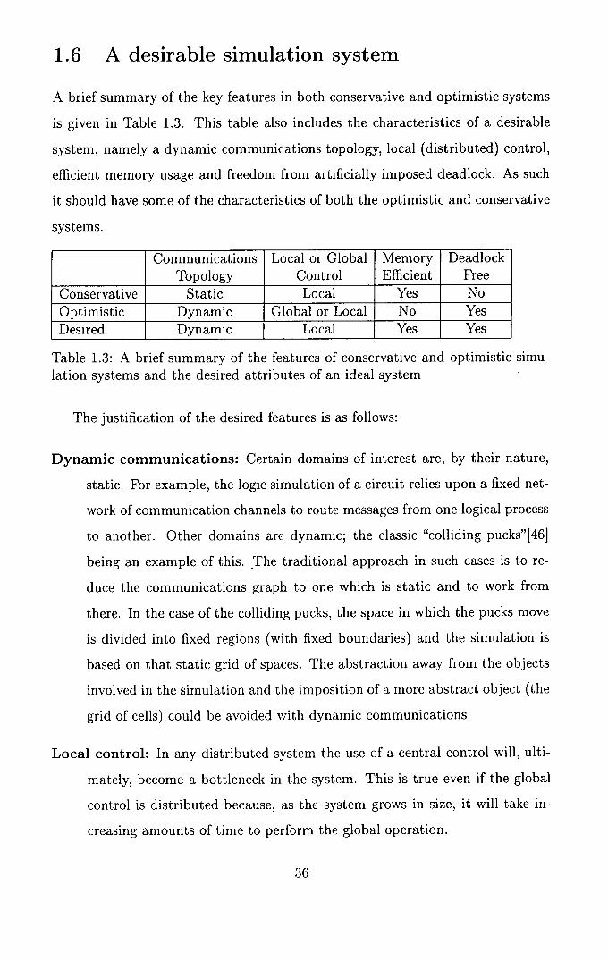
A brief summary of the key features in both conservative and optimistic systems
is given in Table 1.3. This table also includes the characteristics of a desirable
system, namely a dynamic communications topology, local (distributed) control,
efficient memory usage and freedom from artificially imposed deadlock. As such
it should have some of the characteristics of both the optimistic and conservative
systems.
Communications Topology
Local or Global Control
Memory Efficient
Deadlock Free
Conservative Static Local Yes No Optimistic Dynamic Global or Local No Yes Desired Dynamic I Local j Yes Yes
Table 1.3: A brief summary of the features of conservative and optimistic simu-lation systems and the desired attributes of an ideal system
The justification of the desired features is as follows:
Dynamic communications: Certain domains of interest are, by their nature,
static. For example, the logic simulation of a circuit relies upon a fixed net-
work of communication channels to route messages from one logical process
to another. Other domains are dynamic; the classic "colliding pucks"[46]
being an example of this. The traditional approach in such cases is to re-
duce the communications graph to one which is static and to work from
there. In the case of the colliding pucks, the space in which the pucks move
is divided into fixed regions (with fixed boundaries) and the simulation is
based on that static grid of spaces. The abstraction away from the objects
involved in the simulation and the imposition of a more abstract object (the
grid of cells) could be avoided with dynamic communications.
Local control: In any distributed system the use of a central control will, ulti-
mately, become a bottleneck in the system. This is true even if the global
control is distributed because, as the system grows in size, it will take in-
creasing amounts of time to perform the global operation.
36
Memory efficient: Memory is relatively cheap and modern machines come with
many times the memory available ten years ago. However, ultimately the
amount of memory is still a limited resource which needs to be husbanded
and allocated sparingly. If a system is not efficient in its memory use,
there is also the possibility that accessing the data in memory will take
up an increasing amount of time, either because the data is held in virtual
memory which needs to be paged in from disk or because the data structure
holding the desired information takes times to traverse to locate the actual
piece of data desired.
Processor efficient: Processor power is increasing but so is the expectation of
what that resource can do for the user. It is important therefore, that the
simulation system is efficient in the use of what processor power is available.
Deadlock free: By this we mean that the simulation system should not intro-
duce deadlock where none exists in the real system. Should the protocol
under which the simulation is being performed be susceptible to deadlock
then steps must be taken to either prevent or to detect and resolve deadlock
within the protocol. Any such activity will introduce an overhead into the
system which detracts from the system performing useful simulation work.
1.7 Problem to be addressed in this thesis
In this thesis we shall develop a simulation system which has the following fea-
tures:
• Dynamic communications
• Local control
• Resource efficient
• Deadlock free
• Conservative
37

. Distributed
. Able to exploit both temporal and structural parallelism
We shall show models of the upper bound of resource consumption (both
processor time and bandwidth) as well as experimental results for the simulation
of a number of synthetic and real-world systems.
In this chapter we have surveyed the state of the art in distributed simulation
and covered the characteristics of the two main systems (conservative - Chandy-
Misra-Bryant and optimistic - Time Warp). We note that neither of these systems
has all of the attributes of the desired simulation system.
In the next chapter we outline a system which has the desirable features listed
above and set the context in which the system was developed.
RN
Chapter 2
Background
In Chapter 1 we looked at the advances made in parallel and distributed simula-
tion from the early conservative CMB systems through the optimistic, or Time-
Warp, systems to the various attempts to unify the simulation synchronisation
process. We ended the chapter by outlining, and motivating, the features desired
in a distributed simulation system.
In this chapter we step back from simulation and look at the more generic
problems of the production and synchronisation of data in distributed systems,
and how it relates to the desirable features listed in Table 1.3.
2.1 An Approach to the Obtaining the Desirable Features
In conservative CMB-style simulation each LP in the system must determine its
state for every moment in the simulation. The optimistic Time Warp approach
requires that every LP determine its state for every moment during the simulation
but also permits the LP to process messages out-of-order and thus potentially
erroneously. Should a causality error occur, the LP is then forced to re-evaluate
some of its history. Thus, a LP can do more computation than is necessary. This
style of processing has been defended by saying "whenever rollback occurs, other
rollback-free implementations would require blocking for an amount of real time
equal to that spent on wasted computation"1451. In other words, no "useful" time
was wasted. While this held true when the user was allocated a specific number
of processors for their sole use, increasingly, parallel machines are being created
39
which permit the sharing of processors by more than one user. The obvious
example of such a system is a network of workstations. In these shared multi-
processor systems, computation time taken by one user is denied to another.
Furthermore, it is not always necessary for every LP to know the state of all
its inputs for the output result to be determined. Consider, for example, the
multiplication of two numbers. Should one number be known to be zero then the
other number need not be determined as the result is also zero. Any processor
time not used by one user is available to another. The trade-off at issue is the
speed of completing one job versus the total throughput of the system.
The problem therefore is how to design a simulation system which permits
the result to be obtained by computing only the necessary values.
2.2 Distributing data
The core feature underlying all of distributed computation and, specifically, dis-
tributed simulation is the ability to coordinate the production, delivery, and con-
sumption of data'. We will use these aspects to derive a protocol with some of
the desired features listed in Table 1.3. By "data" we mean discrete packets of
information which are complete within themselves.
The problem of distributing data can be split into two separate parts: where to
send the data (distribution) and when to create and send the data (production).
The case where the location and the time are not independent can be addressed by
sending the data to a redirection process at a fixed location which then forwards
the data to the appropriate location. This thus reduces the problem to the first
case. Maintaining the redirection, or directory, service is outwith the scope of
this thesis and does not form part of the argument.
'There are some systems in which the data remains in a fixed location and the processing code moves to it rather then the other way around. An example of such a system could be an image analysis application in which, due to the amounts of data to be processed, it is easier for the desired transform to be sent from processing element to processing element than for the image data to be sent.

2.2.1 Data distribution
All data which is to be distributed must have some condition attached to indicate
when the data has either reached its desired destination, or is to stop looking.
What this implies is that the destination of the data packet must be known before
it is sent and is thus under the control of the sending process.
In the case of conservative algorithms, the sending process knows the desti-
nation as the topology of the processing elements is fixed. Data packets, once
produced, can only be sent to a subset of the processing elements.
In the case of the optimistic algorithms, the sending process knows the desti-
nation as it knows the location of all the processing elements in the system. Data
packets, once produced, can be sent to any of the processing elements.
While the optimistic algorithms provide for a dynamic topology, the conserva-
tive systems do not. One solution to the problem of providing a dynamic topology
to the conservative algorithms would be to have a completely connected set of
processes and to have each process broadcast its data packet to the rest of the
system. While such a system might work, it is impractical as the number of con-
nections needed would grow exponentially in the number of processing elements
in the system. What is needed is some way of the sending element knowing which
of the possible elements in the system need to receive the data.
2.2.2 Data production
The question also arises of when to produce a new data packet for distribution.
The conservative system will only create a data packet when it has sufficient
information to determine the contents of that data packet. An optimistic system,
on the other hand, will only create a new packet if a change to one of the input
values results in a change to the output value. For the sake of simplicity, we will
ignore the messages created to effect a rollback should a causality violation occur.
Both of these systems generate data for distribution irrespective of whether
or not the data is required by the rest of the system. What is needed is some way
for an element in the system to indicate from which other elements it needs fresh
data.
41
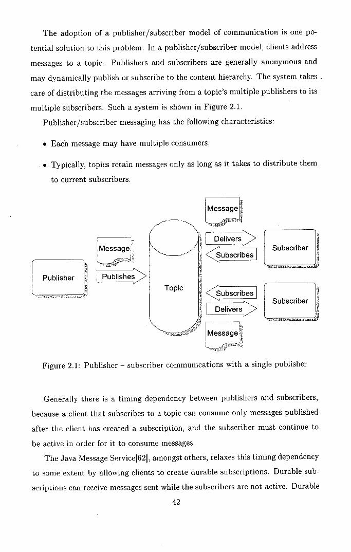
ssa
Lver
T ribes
<jribes
L rs Delive
r 1i Subscriber
r Subscriber I
to current subscribers.
1 Publisher
Message
Topic
The adoption of a publisher/subscriber model of communication is one po-
tential solution to this problem. In a publisher/subscriber model, clients address
messages to a topic. Publishers and subscribers are generally anonymous and
may dynamically publish or subscribe to the content hierarchy. The system takes
care of distributing the messages arriving from a topic's multiple publishers to its
multiple subscribers. Such a system is shown in Figure 2.1.
Publisher/subscriber messaging has the following characteristics:
. Each message may have multiple consumers.
• Typically, topics retain messages only as long as it takes to distribute them
Essa Figure 2.1: Publisher - subscriber communications with a single publisher
Generally there is a timing dependency between publishers and subscribers,
because a client that subscribes to a topic can consume only messages published
after the client has created a subscription, and the subscriber must continue to
be active in order for it to consume messages.
The Java Message Service[621, amongst others, relaxes this timing dependency
to some extent by allowing clients to create durable subscriptions. Durable sub-
scriptions can receive messages sent while the subscribers are not active. Durable
42
subscriptions provide the flexibility and reliability of queues but still allow clients
to send messages to many recipients. While most messaging systems, not unsur-
prisingly, use real time as the temporal measure when assessing whether or not
a subscriber can receive a particular message, there would be no great difficulty
in using the simulation (or virtual) time in the same way. This would permit a
client to subscribe to the topic for a virtual time interval.
2.2.3 A potential solution
From the previous section we saw that a system where the individual elements
could indicate from which elements they required data, and also when they re-
quired that data, would meet some of the requirements of our "ideal" system;
providing a dynamic topology as well as local control. We have, in effect, added
the ability to provide a dynamic topology to a conservative system.
Now that a dynamic topology is available, a potential solution presents itself
from the wording of the problem. We require a system which would only compute
those values which were necessary to determine the result. The first step would
therefore be to decide what values are necessary and then to determine those
values. This leads to a reversal of the standard data-driven method whereby the
data is produced and promulgated with the assumption that it will be necessary.
Such systems, known as demand-driven systems, have other properties which will
be expanded on in Chapter 3.
2.3 Related work
There is little related work addressing simulation per se. Demand driven evalu-
ation, and its close relation lazy evaluation, have been studied at various levels
from instruction level, through compiler level, to user exposure in languages. In
this section we will look at each of these levels.
2.3.1 Request Driven v's Demand Driven
The terms "request driven" and "demand driven" are sometimes used by different
authors to mean the same thing. This is unfortunate as they are also used, by
43
other authors, to indicate different methods of computation.
In order to avoid adding to this confusion, we will clarify what we mean by
request and demand driven evaluation.
Request driven: In a request driven system, the client requests that the data
be provided when it is available. In effect, it notifies interest in the result when it
becomes known. This is the default mode of operation of the publisher/subscriber
model.
Demand driven: In a demand driven system, the client demands that the
data be provided as soon as possible. If the data is available, then this is the
same as request driven. Should the data not be available, a demand driven
system requires the publisher to take action to produce the data (probably by
issuing demands of its own).
The rest of the thesis will focus on demand-driven evaluation and related
ideas.
2.3.2 Micro level
The dataflow model was originally proposed in the mid-60's. Initially the con-
cept of dataflow was expressed as a graph, which later became parallel program
schemesl77, 1, 251. It was later at MIT[26] that designs of actual computers based
on the dataflow model were attempted. Dataflow programs can be described in
terms of directed graphs expressing the flow of data between nodes of the graph,
with a node representing an instruction or a group of instructions [241. Data
are active and flow asynchronously through the program. The original dataflow
model exploits very fine-grain or instruction level parallelism.
The performance of pure, fine-grained, dataflow systems was not able to
compete with von Neumann processors[671 when executing sequential programs.
Arvind[4] identified the real benefits of dataflow systems as cheap synchronisation
and tolerance of memory latency. Hybrid processors that combine features from
both von Neumann and dataflow architectures have been developed[68].
The reduction machine891 is an architecture closely related to the dataflow
model. Reduction is based on the demand driven principle and supports func-
tional languages. Beginning at the outermost expression of a functional program,
sub-expressions within an enclosing expression are recursively reduced upon de-
mand for their results, into simpler forms, until the expression cannot be further
reduced (known as normal form). The reduction process involves rewriting re-
ducible expressions by others with the same meaning until a constant expression
representing the result of the program execution is reached. This contrasts with
the data-driven model (upon which datafiow is based) which starts execution
on the innermost expressions that have their values and propagate the results
into the expressions requiring them. One can view the demand-driven and data-
driven program graph for the same expression as being identical, except that the
direction of the links is reversed. The execution graph of a demand-driven eval-
uation is dynamically changing during execution, whereas the program graph of
the datafiow evaluation is static.
2.3.3 Compiler level
The use of demand-driven (lazy) evaluation can be at a higher level than the
processor. A number of languages have been designed to take advantage of lazy
evaluation without providing specific constructs to the user. In general, such
languages were categorised as non-strict.
In a non-strict language, the arguments to a function are not evaluated until
their values are actually required. For example, evaluating an expression of the
form f(exp) may still terminate properly, even if evaluation of exp would not, if
the value of the parameter is not used in the body of f. Miranda and HaskellE101
are examples of this approach.
In a strict language, the arguments to a function are always evaluated before
it is invoked. As a result, if the evaluation of an expression exp does not terminate
properly (for example, because it generates a run-time error or enters an infinite
loop), then neither will an expression of the form f(exp). ML and Scheme are
both examples of this.
There is much debate in the functional programming community about the
relative merits of strict and non-strict languages. It is possible, however, to
45
support a mixture of these two approaches; for example, some versions of the
functional language Hope do this.
2.3.4 Language level
Halstead[40, 391 proposed a language construct called a future. The construct
allows programmers to explicitly expose parallelism, with minimal effort, in ap-
plicative languages such as MultiLisp. The form (future X) immediately returns
a future, and creates a task to evaluate X. Rather than waiting for the result of
such a computation, the program receives a "placeholder" for that result and is
able to continue executing. The placeholder behaves just like any.other variable
until an attempt is made to use its value; at that point, if the computation is not
finished then the thread of execution trying to obtain the value will be blocked
until the value is ready.
The principal design rationale behind futures, stated by Mohr et al.[61], is
that "the programmer takes on the burden of identifying what can be computed
safely in parallel, leaving the decision of exactly how the division [of work] will
take place to the runtime system". The Mohr paper goes on to discuss lazy task
creation which would be evaluated when needed, which brings us back round to
demand driven systems.
The future construct is no longer restricted to the applicative programming
domain. Wagner[921 has created portable futures in C++.
It is interesting to note that the simulation of logic circuits was used as a test
example to show the power of this construct on a multi-processor machine[111.
2.3.5 Demand driven Simulation
Most of the papers dealing with demand driven simulation have been quite firmly
rooted in the domain of logic simulation. A number of them state that demand-
driven evaluation can be easily expanded to a larger class of systems but fail to
address the issues involved, such as function re-evaluation and random number
generation. The results of most functions are deterministic. Random number
servers are, hopefully, non-deterministic. Any attempt to re-evaluate a random

Circuit "unoptimised" evaluation elapsed time ratio
"optimised" evaluation elapsed time ratio
74181 ALU 0.434 0.238 C432 0.605 0.284 C499 0.647 0.525 C880 0.607 0.463 C1355 0.747 0.616 C1908 0.864 0.637 C2670 0.954 0.534 C3540 1.296 0.398 C5315 1.247 0.444 C7552 1.337 0.740
Table 2.1: Ratios of Demand driven simulation to event driven simulation
number function must produce the same number as the initial request.
The earliest paper that can be found relating demand-driven evaluation and
simulation is by Smith et al.[81]. The paper presents a sequential algorithm for
the simulation of digital logic circuits and compares it with a standard event
driven algorithm. The test circuits used are those which were created for the
International Symposium on Circuits and Systems, 1985[12] which have since be-
come the closest thing to a standard benchmark circuit that the logic simulation
community has. Two different evaluation models are presented. The first is a
standard event driven evaluation model. The second has a number of optimisa-
tions applied; most notably early cutoff (evaluation stops as soon as the result
is known). The optimised system consistently out-performs the standard event-
driven approach. A table of the results is shown in Table 2.1.
It should be noted that this paper, and other results by the same author,
describe a system which uses requests, not as the main driving force behind the
simulation, but as a way to ensure that the simulation proceeds; should an input
not have a current message, a request is sent asking for the data tobe forwarded.
A second report by Smith[801 expands on his earlier work and includes, for the
first time, a notion of time windows which encompass a number of discrete-event
time units. Using the same test circuits as were used in the earlier paper described
above, a number of experiments were conducted to determine the effect of various
47
modification to the algorithm. As a base case for comparisons, the system is
compared with a standard event driven algorithm where both simulators use the
same evaluation routine. The demand driven system is then modified to include
early cutoff in its evaluation. A further experiment is made using a number of
heuristics to reorder the input pin evaluation order.
A further modification of the algorithm is given which provides methods for
modelling both transport and inertial delays in logic circuits. This information is
presented in a more general form by Charlton[22] which we will cover later.
Subramanian and Zargham[87] move demand-driven simulation explicitly into
a parallel arena for the first time. Three different algorithms are used for com-
parison purposes. The first of these is a discrete event system similar to the
CMB algorithm[19. The second is a pure demand-driven system (DD) and the
third is an algorithm with two phases: the earlier phase determines which input
values will be needed using a demand-driven approach and the later phase then
evaluates in a standard CMB manner. The results show that the pure demand
driven system performs better than either the CMB system or the two-phase sys-
tem. The circuits used are not described or attributed with only the number of
elements used and the type of the circuit (sequential or combinatorial) stated.
There has been some work performed by Chariton et al. on demand-driven
simulation of logic circuits[211. Most of their work derives from studies of lazy
evaluation. The earliest paper investigates the effect of differing event scheduling
strategies for both demand and event driven systems. It shows that significantly
fewer events need to be processed with a demand driven system. The results are
based on a uniprocessor simulator with a single queue.
Charlton[221 demonstrates a method for modelling general delays in demand-
driven simulation. Basically, assuming a node has a maximum (minimum) delay
Of tmax (t m in ) then a request for data for an interval (a,b) is fulfilled by a request
for data in the interval (a - tmax ,b - tmin) as this interval will always be sufficient
to determine the input values for whatever the actual delay turns out to be. This
work is presented in relation to a system which is being driven by time-stamped
requests and not intervals.
Both of the above papers have addressed issues from the perspective of unipro-
cessor simulation. Another paper from the same group[30] covers parallel evalu-
ation strategies for demand-driven simulation. Optimal evaluation orderings are
obtained for a number of basic two input logic functions assuming that two pro-
cessors are available to evaluate the function. Heuristics are then developed which
make implementation more practical. Results obtained show that the heuristics
perform no worse than 1.6 times slower than the optimal strategies.
Only one of the papers surveyed deals with the evaluation of abstract simula-
tion models[631. The models are built in Miranda and then different simulation
evaluation strategies are applied to the models. It concludes that the demand
driven system is inefficient in both space and time and that a discrete event (data
driven) system can deal with all inefficiencies. It also states that the demand
driven system is less expressive as it cannot model inertial delays. This has been
shown to be incorrect in the work of Charlton[22]. It closes by stating that as
demand driven systems are inefficient they are easy to parallelise. A number of
the criticisms targeted at demand driven simulation are addressed in Chapter 3.
2.4 Speedup and Efficiency
When assessing the quality of the performance of a parallel system, two measures
have often been used. The first, speedup, indicates how much faster the result
is obtained as the number of processes increase (Equation 2.1). The numerator,
T1 , is sometimes the time taken by the best possible sequential solution, but is
generally taken to be the time for the parallel code running on a single processor.
The denominator, T, is the time taken when using n processors.
S(n)= T. (2.1)
The second measure, efficiency, is defined as the average utilisation of the ri
allocated processors. Ignoring I/O, the efficiency of a single processor system is
equal to one. The relationship between speedup and efficiency is given by
E(n) = S(n) (2.2)
Eager et al. [321 argue that these measures can be used to determine an "opti-
mal" number of processors to be used in the execution of a given problem. They
plot a measure of "benefit" (execution time) against a measure of "cost" (number
of processors) and note that a knee occurs in the graph. The knee is the point
where the benefit per unit cost is maximised and which, intuitively, represents
an optimal system operating point. They argue that being able to estimate the
number of processors that yields the knee is important as that would indicate the
appropriate allocation of processors for that job.
While these measures have relevance in the multi-programmed, multiproces-
sor with a static processor allocation, their use in a network-of-workstations en-
vironment is less clear as they only take into account real cost (the resources
consumed).
2.4.1 Opportunity cost
Opportunity cost is a basic term from the disciplines of economics and ac-
counting. In these circles the acceptable definition of the term is, "the advantage
forgone as the result of the acceptance of an alternative".
In assessing the efficiency of a system the opportunity cost has often been
ignored. This stems from the understanding that a system needs certain resources
before it can start and holds them until it is finished. In machines with a static
allocation of processors, this is the natural state of affairs. Such a situation does
not hold true in multiprocess systems where an individual process will only reserve
a resource for the duration needed. It might claim and release that resource many
times during the its lifetime. An example would be time-slicing CPU access on a
multiuser system.
Opportunity cost is a relative measure in that it compares what is with what
could have been. As such care must be taken in its use to avoid trying to compare
the incomparable.
50
2.5 Binary Decision Diagrams
Before we leave this chapter, it is useful to take a look at how boolean functions
can be represented using binary decision diagrams (BDD)[14], and in particular,
Ordered Binary Decision Diagrams (OBDD)[15]. It should be noted that the use
of BDD is not needed for a demand-driven system to function, but they can be
used to make clear some of the benefits of a demand-driven system.
Binary decision diagrams have been recognised as abstract representations
of Boolean functions for many years[3]. A binary decision diagram represents a
Boolean function as a rooted, directed acyclic graph.
A binary decision tree is formed by expanding the binary expression around
a single variable and then repeating for each sub-expression until there is no
expression left to evaluate.
Consider the expression
f(A,B,C) =ABCVAC
This expression could be expanded as follows 2 :
f(A, B, C) = A(f(1, B, C)) V A(f(O, B, C))
This could be repeated for the variables B and C.
A graph of the resulting tree is shown in Figure 2.2.
Each non-terminal vertex is labelled with a variable var(v) and has arcs di-
rected to two children: lo(v) corresponding to the case where the variable is
assigned the value 0 and hi(v) corresponding to the case where the variable is
assigned the value 1.
2.5.1 Reducing the tree
This naïve representation provides 2n paths from the root to the leaves, one for
each of the 2fl different combinations of input values. A number of reductions can
be applied to reduce the number of available paths.
2 This identity is known as the Shannon expansion of f with respect to A, although it was
originally recognized by Boole
21 C2:J
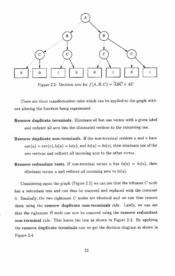
Figure 2.2: Decision tree for f(A, B, C) = ABC V AC
There are three transformation rules which can be applied to the graph with-
out altering the function being represented:
Remove duplicate terminals. Eliminate all but one vertex with a given label
and redirect all arcs into the eliminated vertices to the remaining one.
Remove duplicate non-terminals. If the non-terminal vertices u and v have
var(u) = var(v), lo(u) = lo(v), and hi(u) = hi(v), then eliminate one of the
two vertices and redirect all incoming arcs to the other vertex.
Remove redundant tests. If non-terminal vertex u has lo(u) = hi(u), then
eliminate vertex u and redirect all incoming arcs to lo(u).
Considering again the graph (Figure 2.2) we can see that the leftmost C node
has a redundant test and can thus be removed and replaced with the constant
0. Similarly, the two rightmost C nodes are identical and we can thus remove
them using the remove duplicate non-terminals rule. Lastly, we can see
that the rightmost B node can now be removed using the remove redundant
non-terminal rule. This leaves the tree as shown in Figure 2.3. By applying
the remove duplicate terminals rule we get the decision diagram as shown in
Figure 2.4.
52
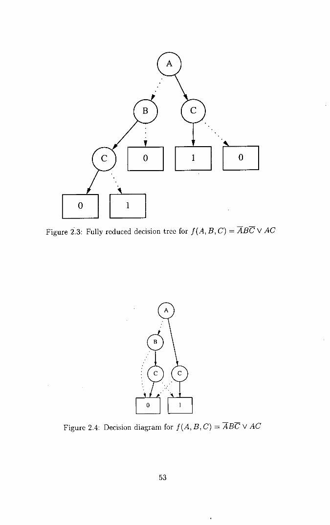
r.
Figure 2.3: Fully reduced decision tree for f(A, B, C) = ABC V AC
B
Hit Figure 2.4: Decision diagram for f(A, B, C) = ABC V AC
53
2.5.2 Combining diagrams
Each binary decision diagram represents a boolean function and can be created
by combining simpler boolean functions in the manner described below.
First, an explanation of some notation. Consider a function f which takes a
vector ±' then the notation
f Ix i - o
means the function with the value of x i set to the constant 0. This is sometimes
referred to as restriction.
Now, the combination of two functions f and g by the operation <op> can
be defined as
f < op > g = .( fIx4-o <op> gI-o) + x.(f+1 <op> 9x-1)
This technique will provide an algorithm for computing f <op> g with a time
complexity which is exponential in n (the number of inputs). There are various
methods and improvements to the algorithm which reduce this complexity[ 14, 15].
2.6 Attributes of Decision Diagrams
Decision diagrams have a number of attributes which make them useful in demand
driven evaluation.
2.6.1 Automatic short circuiting
Functions can be split into three classes.
Strict: These functions always require all of their inputs before they can eval-
uate an output, e.g. addition.
Partially strict: These functions may require all of their inputs before they can
evaluate an output, e.g. multiplication (when one input is zero).
Non-strict: These functions never require all of their inputs before evaluat-
ing an output, e.g. if. . . then. . . else. . . Either the then branch needs to be
evaluated or the else branch, but never both branches.
54
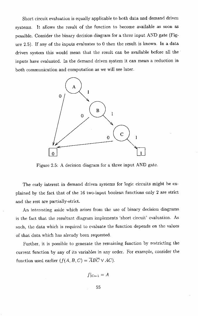
ME
0
QB I
Short circuit evaluation is equally applicable to both data and demand driven
systems. It allows the result of the function to become available as soon as
possible. Consider the binary decision diagram for a three input AND gate (Fig-
ure 2.5). If any of the inputs evaluates to 0 then the result is known. In a data
driven system this would mean that the result can be available before all the
inputs have evaluated. In the demand driven system it can mean a reduction in
both communication and computation as we will see later.
0/ 1: 1 ,
Figure 2.5: A decision diagram for a three input AND gate.
The early interest in demand driven systems for logic circuits might be ex-
plained by the fact that of the 16 two-input boolean functions only 2 are strict
and the rest are partially-strict.
An interesting aside which arises from the use of binary decision diagrams
is the fact that the resultant diagram implements 'short circuit' evaluation. As
such, the data which is required to evaluate the function depends on the values
of that data which has already been requested.
Further, it is possible to generate the remaining function by restricting the
current function by any of its variables in any order. For example, consider the
function used earlier (f (A, B, C) = ABC V AC).
f Ic+-i = A
55
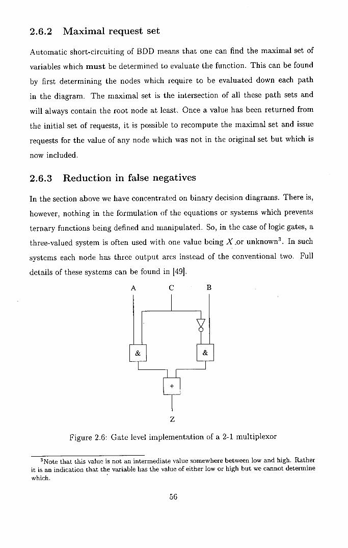
2.6.2 Maximal request set
Automatic short-circuiting of BDD means that one can find the maximal set of
variables which must be determined to evaluate the function. This can be found
by first determining the nodes which require to be evaluated down each path
in the diagram. The maximal set is the intersection of all these path sets and
will always contain the root node at least. Once a value has been returned from
the initial set of requests, it is possible to recompute the maximal set and issue
requests for the value of any node which was not in the original set but which is
now included.
2.6.3 Reduction in false negatives
In the section above we have concentrated on binary decision diagrams. There is,
however, nothing in the formulation of the equations or systems which prevents
ternary functions being defined and manipulated. So, in the case of logic gates, a
three-valued system is often used with one value being X or unknown'. In such
systems each node has three output arcs instead of the conventional two. Full
details of these systems can be found in [491.
A C B
z
Figure 2.6: Gate level implementation of a 2-1 multiplexor
'Note that this value is not an intermediate value somewhere between low and high. Rather it is an indication that the variable has the value of either low or high but we cannot determine which.
56
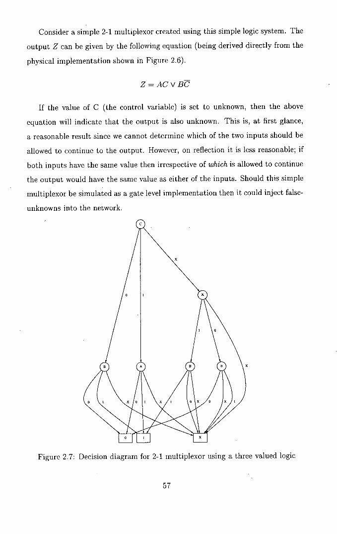
Consider a simple 2-1 multiplexor created using this simple logic system. The
output Z can be given by the following equation (being derived directly from the
physical implementation shown in Figure 2.6).
Z=ACvBC
If the value of C (the control variable) is set to unknown, then the above
equation will indicate that the output is also unknown. This is, at first glance,
a reasonable result since we cannot determine which of the two inputs should be
allowed to continue to the output. However, on reflection it is less reasonable; if
both inputs have the same value then irrespective of which is allowed to continue
the output would have the same value as either of the inputs. Should this simple
multiplexor be simulated as a gate level implementation then it could inject false-
unknowns into the network.
Figure 2.7: Decision diagram for 2-1 multiplexor using a three valued logic
57

However, should the multiplexor be implemented as a single unit with a func-
tion derived from the decision diagrams for the three gate implementation, these
false-unknowns will not occur. The diagram is shown in Figure 2.7.
2.7 Chapter Summary
In this chapter we stepped back from simulation and looked at the more generic
problems of the production and synchronisation of data in distributed systems.
We saw that, by making the receiver responsible for requesting the data rather
than have it wait passively, we could obtain a dynamic topology for inter-element
connections.
We clarified the difference between request driven and demand driven system
and looked at related work at the micro, compiler and language levels. Work
in simulation, using either demand driven or request driven systems, was also
discussed.
We looked at the definitions of speedup and efficiency that are widely used
throughout the distributed systems field as quality measures and proposed a new
measure, opportunity cost, which gives an indication of how much of the systems
resources are withheld from other potential users.
We closed the chapter by looking at binary decision diagrams. This method
of expressing a function can make explicit any non-strictness in that function and
as such, is well placed to be utilised in a demand driven system.
In the next chapter we take the results from our investigation and propose a
demand driven simulation system.
The insights obtained will then be used to address the requirements of our
desired simulation system.
I
Chapter 3
Demand-Driven Simulation
This chapter discusses some of the costs and benefits associated with demand-
driven simulation. The costs are resource consumption, be they bandwidth, pro-
cessor or time. It provides arguments in mitigation of a number of the costs
involved as well as strategies to reduce the overall cost of simulating a system.
3.1 Costs and Benefits of Demand-Driven Simu-lation
Parallel discrete event simulation has been data driven since its inception. This
can be considered a logical progression from the sequential simulation systems
where there existed a queue of events which needed to be processed. The key word
in the previous sentence was "needed". One problem with data driven systems
is that events will be generated which will have no effect on the receiving node
and therefore, for efficiency reasons, need not have been generated in the first
place. Unfortunately the logical process which generated the event could not
have foreseen this and hence the event has to be generated "just in case".
The underlying idea is that the system under simulation is a "black box"
which is exercised by a series of data values and the changes in outputs are
observed. Demand-driven systems reverse this concept; the output is interrogated
and demands for data propagate up the system and back in simulation time until
a demand is made of the input data pool. Since in a demand driven system logical
processes only generate an event when the receiving node requests it, potentially
only the minimum amount of work needs to be performed.
59

The biggest potential problem with standard demand driven systems is that
for each event needed two messages must be sent; one to request the event and
the event itself. In parallel systems, where communications are generally much
slower than computations, this could appear to be a significant problem. The
effect might be mitigated by the decreased computation required as only necessary
work is performed. We term this "the doctrine of necessary computation".
3.1.1 The Costs
A number of costs are associated with demand driven simulation which are not
associated with data driven simulation. In this section these costs are analysed
and evidence presented of ways in which these costs might be mitigated.
3.1.1.1 Communication costs
There is an obvious problem with such a demand driven system: extra commu-
nication. The most glaring inefficiency, and the one which is most often stated as
a reason for not using this method, is the extra communication which is required
to "spark" the computation. In the worst case each data value will require twice
the number of communications than it would under a data driven system. A
point to make about this observation is that it is the number of communications
which would, at worst, double and not the communication load itself. If we use
the simple equation a+/31, where a is the start-up cost for communication, 0 the
cost per unit transmitted and I is the message length then the actual overhead is:
2a+0(Id+I)
a + 131d
where 1d is the length of the data message and 1, is the length of the request
message.
If we assume that the size of the request message is smaller than the size of
the data message then the overhead must be strictly less than a factor of 2. If we
assume that a request message is significantly smaller than a data message, the
equation can be written as
2- I31d (3.1) a + I31d
60
This approximation to the overhead factor can be analysed by cases.
a >> Old The start-up cost is significantly larger than the transport cost. This
situation could occur if a large number of small messages were to be sent.
The overhead tends towards a factor of 2.
a = Old The start-up costs and the transport costs are equal. The overhead is a
factor of 1.
a << Old The start-up cost is significantly smaller than the transport costs. This
situation could occur if large messages were to be sent. The overhead tends
towards a factor of 1. In other words, as the size of the data message
increases, the request induced communication cost as a fraction of the total
communication cost falls.
There are further techniques which can be employed to reduce the communi-
cation traffic. The simplest technique is to bundle a number of requests into a
single message. The practicality of this method will depend upon the time ad-
vance mechanism in the simulation. Such a system has been used in data driven
time warp simulation by Butler and Wallentine[16]. They show that bundling
events into a single message can reduce the communications load but that the
benefit varied with cancellation strategy. If we assume that the simulation is
interval based, as for ELSA [5, 6], then a number of requests for consecutive in-
tervals can be compressed into a single message no larger than a single request.
ELSA is explained in greater detail in Chapter 4.
3.1.1.2 Computation costs
The next cost to be considered is an increase in work required at a logical pro-
cess. Every message which arrives at a logical process must be handled. This
is produced by the requirement to handle incoming request messages as well as
data messages. Again, the doctrine of necessary computation can help to reduce
this overhead as fewer logical processes need to be evaluated. The result could
be that the computation load is concentrated on fewer logical processes than in
the equivalent data driven system.
61
3.1.1.3 Memory costs
Memory requirements may rise because of the requirement of some types of node
to store their previously computed data. In the case of a random number gen-
erator it might be desirable for every node which requests its state at time t to
be given the same answer. The use of MEMO functions has been studied in the
realm of functional programming[58, 43]. The idea behind them is very simple: a
memo-function is like an ordinary function, but it remembers all the arguments
it is applied to, together with the results computed from them. If it is ever
re-applied to an argument the memo-function does not recompute the result, it
just re-uses the result computed earlier. "Memoisation" is an optimisation which
replaces a potentially expensive computation by a simple table look-up.
One of the difficulties in implementing general memo functions arises from
the need to determine whether two calls to the same function are equivalent. In
a general solution, comparing data-structures for equality is expensive. It is not
uncommon for a conservative definition of equality to be used for the test. Two
objects could be tested for identity as follows:
If they are stored at the same address, then they are identical. Return true.
If they are atomic values (such as numbers, booleans, characters) then they
are identical if they are equal.
Otherwise they are not identical. Return false.
Fortunately in demand driven simulation the inputs to any logical process are
tagged with their time. Therefore the task of determining whether two inputs
are identical reduces to comparing their associated times. As demand driven
simulation has no concept of "fossil collection" which is common in timewarp
systems to manage memory, it would be possible for these memo stores to grow
throughout the simulation run. This might be desirable as it would provide a
record of the state of the logical process throughout the simulation. This may be
of great use in a postmortem of the simulation run.
However, in cases where we are only interested in the final value and not
in the intermediate results we can consider these memo stores to be, in effect,
62
caches. As such certain cache replacement algorithms could be employed to limit
the memory requirement. The commonly applied LRU algorithm where the least
recently used block is replaced might be used effectively, but this requires further
investigation.
3.1.2 The Benefits
The use of demand driven simulation is not without qualitative benefits. An
important benefit is that the logical processes in the system under consideration
are able to dynamically reconfigure their local network in order to contact any
other logical process. Below we describe five benefits of using demand-driven
evaluation.
"Necessary" Computation: each node in the system makes only those requests
which it deems necessary. This means that if the value of an input is not
required then it is not evaluated. What input values are required can depend
on the values of the other inputs. For example, (A or B), if A is evaluated
and returns 0 then B must be evaluated. If B returns 1 then the answer
could have been found by only evaluating B. So "necessary" computation
does not mean minimal computation.
Dynamic Interconnect: the requesting logical process (LP) is free to commu-
nicate with any other LP in the system. As such the connections are gen-
erated at run time and are able to respond to data dependent conditions.
This could be considered as a global all-to-all topology but with the addi-
tion that each LP is only dependent on a certain sub-set of processes and
are not constrained to the "lock step" that such a configuration would tend
to produce in data driven systems.
Sub-system Activation: to investigate a part of a system it is now only nec-
essary to send a request to that sub-system. The doctrine of necessary
computation results in only those parts of the system which need to be
activated being computed.
63
Realistic Data: one of the major problems in simulating a component of a sys-
tem is generating realistic input data. The difficulty is that realistic data
comes from activating the whole system at a specific level of abstraction and
this can be too computationally intensive to achieve. In a request driven
system only those elements which are required are activated and thus po-
tentially fewer nodes need to be computed to provide realistic data.
Static graph emulation: a graph which is known to be static throughout the
simulation run can be modelled. The number of extra messages is propor-
tional to the number of edges in the static system. Each edge is initialised
to carry a message requesting data from the start of time to the end of sim-
ulation time. The request driven system will now behave as a data-driven
system.
The most striking, and potentially the most beneficial, aspect of demand
driven systems is that, as data is only produced on demand, only those units
whose results are needed by the computation are actually evaluated. The result
of this is that the communication and computation costs will be reduced. This
will have a knock-on effect on multiuser systems as they will have more resource
available to them for their tasks. The more unnecessary work that can be avoided
the higher the opportunity cost saving compared to data driven evaluation of the
same system.
3.2 Strictness and Threshold Functions
If all the functions being evaluated by logical processes were strict - each always
needing all their parameters - then the scope for opportunity cost savings would
be reduced (or eliminated altogether). In order to control the strictness more
easily and to evaluate the system for generic functions, it was decided to use
threshold functions.
Me
3.2.1 Threshold Functions
Threshold functions appear in a number of different fields[641 and can exist in a
number of different forms[591. The output of a threshold function is some function
of the sum of its weighted input values. Consider a function with n inputs. The
intermediate value is given by:
k
Y = E wi x X
where Xi is the value of input i, and w i is its weight. The final value is given by
some function F(Y). Different applications of threshold functions use different
decision functions F. We will be using unit weighted, hard threshold functions.
F(Y\_JO ifY<k " ' - 1 otherwise
The threshold value is k. We denote a threshold function of n inputs and a
threshold of k by T1 .
3.2.2 Strictness
We define the strictness of a function as the amount of data which the function
requires, on average, to compute the result. The value of strictness lies in the
interval [0. . . 11. A strictness of 0 would indicate that the function requires no ex-
ternal information to compute a-result. This is equivalent to a constant function.
A strictness of 1 would indicate that the function requires all of its inputs to be
evaluated, every time, before it can correctly generate an output.
The strictness of a function, f, with n inputs, is defined below.
M(f) = C(f)
The function C(f) is the average number of inputs which are evaluated to
compute the function f. If the value of C(f) depends on the order in which the
inputs are evaluated then the strictness measure calculated is with respect to a
particular variable ordering. An overall strictness can be calculated by a weighted
average of this value over all possible orderings of the input variables.
65
3.2.3 Determining C for Threshold Functions
We shall assume that each input is equally likely to evaluate to 1 as it is to
evaluate to 0. Further, we shall note that the order in which inputs are evaluated
does not effect the count calculated.
There are four cases to consider.
T ° - No further inputs need to be computed and therefore the result must
be known. C(Tk° ) = 0.
T' - As the function can be computed when k inputs have evaluated to 1
and the value of k is zero, then the function need not evaluate any more
inputs. C(T0 ) = 0.
T, n < k - As there are no longer sufficient inputs remaining to be eval-
uated to possibly satisfy k then the function must evaluate to 0 without
further work. C(T,) = 0, n < k.
T, n > k - There are n inputs remaining to be evaluated and once an
arbitrary input has been computed then the remaining patterns will be
split into two sections. The cost of evaluating those sections must also be
included. C(Tfl,n > k 1 + c(T:11)±c(T')
0 if n=0 or k0 or n < k C(Tfl
{ 1 + C(T)±C(T')
otherwise
Should an input favour either a zero or a one then the function for C(T)
needs to be expressed in a more general form.
C(Tfl = 1 + P(I. = 1)C(Ti11 ) + P(I, = 0)C(T 1 )
where P(Ij = 1) is the probability that input i evaluates to 1.
Implicit in the above formula is an ordering on the evaluation of the inputs.
When the probability of a one or a zero is the same for all inputs then the order
is unimportant as the end result will be the same. When the probabilities differ
then the result depends upon the order in which the inputs are evaluated. This is
Me
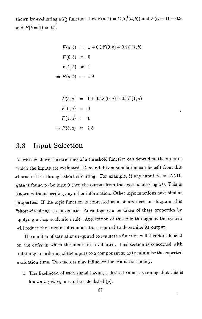
shown by evaluating a T22 function. Let F(a, b) = C(T(a, b)) and P(a = 1) = 0.9
and P(b = 1) = 0.5.
F(a, b) = 1 + 0.1F(0, b) + 0.9F(1, b)
F(0, b) = 0
F(1, b) = 1
=F(a,b) = 1.9
F(b, a) = 1 + O.5F(0, a) + O.5F(1, a)
F(0, a) = 0
F(1, a) = 1
=F(b,a) = 1.5
3.3 Input Selection
As we saw above the strictnessof a threshold function can depend on the order in
which the inputs are evaluated. Demand-driven simulation can benefit from this
characteristic through short-circuiting. For example, if any input to an AND-
gate is found to be logic 0 then the output from that gate is also logic 0. This is
known without needing any other information. Other logic functions have similar
properties. If the logic function is expressed as a binary decision diagram, this
"short-circuiting" is automatic. Advantage can be taken of these properties by
applying a lazy evaluation rule. Application of this rule throughout the system
will reduce the amount of computation required to determine its output.
The number of activations required to evaluate a function will therefore depend
on the order in which the inputs are evaluated. This section is concerned with
obtaining an ordering of the inputs to a component so as to minimise the expected
evaluation time. Two factors may influence the evaluation policy:
1. The likelihood of each signal having a desired value; assuming that this is
known a priori, or can be calculated (p).
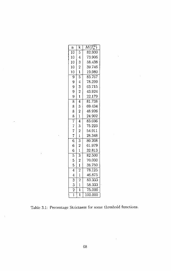
n k M(T,) 10 5 82.930 10 4 73.906 10 3 58.438 10 2 39.746 10 1 19.980
9 5 83.767 9 4 78.299 9 3 63.715 9 2 43.924 9 1 22.179 8 4 81.738 8 3 69.434 8 2 48.926 8 1 24.902 7 4 83.036 7 3 75.223 7 2 54.911 7 1 28.348 6 3 80.208 6 2 61.979 6 1 32.813 5 3 82.500 5 2 70.000 5 1 38.750 4 2 78.125 4 1 46.875 3 2 83.333 3 1 58.333 2 1 75.000 1 1 1 100.000
Table 3.1: Percentage Strictness for some threshold functions.
MWO
2. The expected evaluation time for each signal input (w).
The ordering problem has been analysed for the case of AND gates[79]. The
analysis for OR gates follows easily from this work. The characteristic of an AND
gate which we seek to exploit applies, more generally, to any gate with n inputs
which requires k or more of its inputs to be logic 1 before its output becomes
logic 1, 1 < k < n. Such gates are known as threshold gates. The corresponding
boolean function of ii inputs, Xn =< 1 11 x2 ,.. * ) In >, is denoted by Tkn
Thus TIn is the n-input OR function and Tnn is the n-input AND function. A
circuit whose components are all threshold gates (or their negations) is called a
threshold circuit.
Dunne and Leng[31] expanded on the work of Sassa and Nakata[79] to provide
a general evaluation strategy for threshold circuits. Their work is outlined below.
In order to verify that Tkn evaluates to a logic 1, at least k inputs must be
calculated. The minimum cost of evaluation is obtained by choosing the first k
elements from the order:
WjW Wk - < <...< - Pi Pi Pk
Equally, in order to verify that the function evaluates to a logic 0, at least
(n - k) + 1 inputs must be calculated. The minimum cost of evaluation is obtained
by choosing the first (n - k) + 1 elements from the order:
W . Wi Wk < <...<
1_Pi lPj 'Pk
Note that there is always at least one input which is a member of both sets.
This follows as k elements are in the first selection and (n - k) + 1 elements are in
the second and thus n + 1 elements are represented in total. As there are only n
discrete elements available, at least 1 element must be represented twice. There
may, of course, be more than one element represented twice. We shall call the set
of such elements the Common set.
Once an element from the Common set has been evaluated we are left with
one of two threshold functions depending on the value of the calculated input:
either, T,' if the value is 0 or, T1 if the value is 1. The next input to be
69
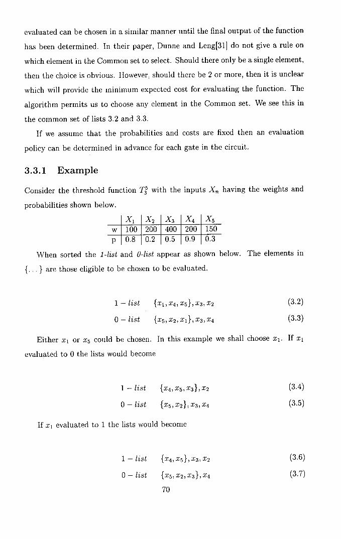
evaluated can be chosen in a similar manner until the final output of the function
has been determined. In their paper, Dunne and Leng[31] do not give a rule on
which element in the Common set to select. Should there only be a single element,
then the choice is obvious. However, should there be 2 or more, then it is unclear
which will provide the minimum expected cost for evaluating the function. The
algorithm permits us to choose any element in the Common set. We see this in
the common set of lists 3.2 and 3.3.
If we assume that the probabilities and costs are fixed then an evaluation
policy can be determined in advance for each gate in the circuit.
3.3.1 Example
Consider the threshold function TI with the inputs X having the weights and
probabilities shown below.
X, x2 x3 x4 x5 W 100 200 400 200 150
p 0.8 0.2 0.5 0.9 0.3
When sorted the 1-list and 0-list appear as shown below. The elements in
{... } are those eligible to be chosen to be evaluated.
1 - list 1x 1 , x 4 , x 5 }, x 3 , x 2 (3.2)
0 - list {x 5 , x 21 x 1 }, x 3 , x 4 (3.3)
Either x 1 or x5 could be chosen. In this example we shall choose x 1 . If x 1
evaluated to 0 the lists would become
1 - list {x 4 , X5, x 3 }, x 2 (3.4)
0 - list 1x 5 , x 2 }, x 3 , x 4 (3.5)
If x 1 evaluated to 1 the lists would become
1 - list {x 4 , x 5 1, x 3 , x 2 (3.6)
0 - list {x 5 , x 2 , x 3 }, x 4 (3.7)
70

If this is repeated, then the resultant tree is shown in Figure 3.1.
Figure 3.1: A minimum expected cost evaluation graph by the method of Dunne and Leng
3.3.2 Remarks
The method described purports to provide an optimal evaluation policy for simu-
lating gates in threshold circuits under certain assumptions. However, the method
is not guaranteed to provide a unique solution and can generate evaluation strate-
gies that, while of low cost, are still sub-optimal. Multiple solutions are available
as a result of non-singleton Common sets.
Another major assumption in the method is that the probabilities associated
with each input are independent. This is only true in tree shaped circuits. Further
it is assumed that the cost of evaluating any input is independent of when it is
evaluated. While this is true in "classic" demand driven systems, any system
which uses memo[431 functions breaks this constraint.
Looking again at Figure 3.1 we note that the immediate children of the root
node are the same. This means that irrespective of the value of input 1 (the root
node), the next input in order to be evaluated is input 5. By waiting for the
value of input 1 before demanding the value of input 5 is, in effect, serialising a
possible parallel operation. We shall look at the opportunities for parallelising
the evaluation of a threshold function in Section 3.4.
71
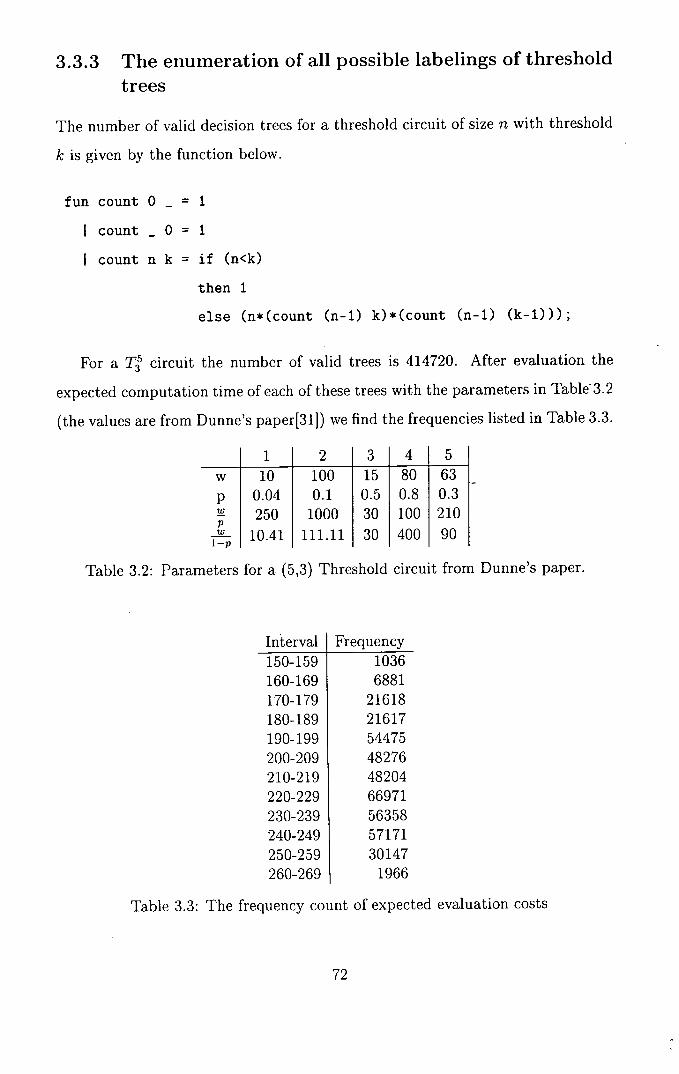
3.3.3 The enumeration of all possible labelings of threshold trees
The number of valid decision trees for a threshold circuit of size n with threshold
k is given by the function below.
fun count 0 - = 1
I count - 0 = 1
I count n k = if (n<k)
then 1
else (n*(count (n-i) k)*(count (n-i) (k-i)));
For a TI circuit the number of valid trees is 414720. After evaluation the
expected computation time of each of these trees with the parameters in Table - 3.2
(the values are from Dunne's paper[311) we find the frequencies listed in Table 3.3.
1 2 3 4 1 5 w 10 100 15 80 63 p 0.04 0.1 0.5 0.8 0.3
250 1000 30 100 210
10.41 111.11 30 400 90
Table 3.2: Parameters for a (5,3) Threshold circuit from Dunne's paper.
Interval I Frequency 150-159 1036 160-169 6881 170-179 21618 180-189 21617 190-199 54475 200-209 48276 210-219 48204 220-229 66971 230-239 56358 240-249 57171 250-259 30147 260-269 1966
Table 3.3: The frequency count of expected evaluation costs
72
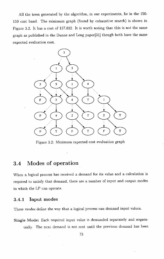
All the trees generated by the algorithm, in our experiments, lie in the 150-
159 cost band. The minimum graph (found by exhaustive search) is shown in
Figure 3.2. It has a cost of 157.032. It is worth noting that this is not the same
graph as published in the Dunne and Leng paper[31] though both have the same
expected evaluation cost.
1
2 l( T
(:~) Z--T Figure 3.2: Minimum expected cost evaluation graph
3.4 Modes of operation
When a logical process has received a demand for its value and a calculation is
required to satisfy that demand, there are a number of input and output modes
in which the LP can operate.
3.4.1 Input modes
These modes define the way that a logical process can demand input values.
Single Mode: Each required input value is demanded separately and sequen-
tially. The next demand is not sent until the previous demand has been
73
satisfied.
Broadcast Mode: This mode sends demands for all the input values that may
be needed to calculate the result.
Parallel Mode: This mode sends demands for all the input values that must be
needed to generate a result.
Group Mode: This mode sends demands for the minimum number of input
values which could generate a result.
These different input modes are best illustrated with an example. Consider
the threshold function TI as defined in Section 3.3.1, one of whose optimum call
graphs is given in Figure 3.1.
Single mode would demand the value of input 1 and then, when the value
arrived, it would follow the appropriate branch and then demand the next value.
In this mode we descend the tree level by level until a fixed value is achieved.
Broadcast mode would demand all the input values-at-once. As the graph has 5
non-leaf levels, all 5 input values would be demanded. As they were returned their
value would replace the node in the graph and incrementally the tree would be
reduced to a fixed value. This may occur before all the results have been returned,
e.g. 1true, 5=true, 4z--true. Subsequent input values can be discarded. The
disadvantage of this mode is that, for non-strict functions, it requires computation
to be performed that is superfluous to the final answer.
Parallel mode attempts to find all those inputs whose value must be known
and then to demand their values in parallel. From the graph (Figure 3.1) we
see that input 1 must be evaluated. We also see that, irrespective of the value of
input 1, the next input that needs to be evaluated is input 5. Parallel mode would
demand the values of inputs 1 and 5 in parallel. As each value was returned, the
call graph would be reduced and, should it be clear that another input must
now be evaluated it will be demanded in parallel with any existing, unsatisfied,
demands. In our example, should node 5 evaluate to false no new demands can
be made (the next input to be evaluated still depends on the value of input 1).
Should input 1 evaluate to true then we can demand the value of input 3 and
74
input 2. We cannot demand the value for input 4 as whether this is needed or
not is dependent on the values of inputs 2 and 3.
The value of a T threshold circuit can be determined by k true values or
(n - k + 1) false values. Let in be the lesser of k and (ii - k + 1). This is the
minimum number of inputs which must be evaluated for the value of the function
to be determined. In our example, m is 3. To determine which inputs to demand
we firstly weight each mode in the call graph with the likelihood that it will be
reached. For each input we sum the weights on all the nodes for the input. In
group mode we request, in parallel, the m inputs with the largest likelihood of
being called. In our example, those are inputs 1, 5 and 2.
The different input modes would be used to evaluate functions in the most
efficient way. If, for example, the function was strict, then all the inputs require
data and so broadcast is the most efficient. If, on the other hand, the function
was non-, or partially-, strict, then a smaller number of data elements might be
required. Single, parallel or group mode could then be more efficient.
3.4.2 Output modes
Just as there are different input modes, so there are different output modes. There
is a complex interaction between the output mode of one logical process and the
input mode of the logical process making the demand.
Demand-response: This mode only allows data to be sent out as a direct result
of a demand for that data. This ensures that the data only reaches those
logical processes that explicitly demanded the data.
Pre-emptive: This mode broadcasts the result to all the logical processes which
might need the result.
Pre-emptive mode does not preclude the demand-response mode. The LPs
which might need the result is based on some predictive model which attempts to
predict future behaviour from observed past behaviour. A simple model would be
to send the data to all LPs that have requested the previous data element. This
model would be self-restricting, in that, should it accurately predict all those LPs
75
which needed the data before the LPs themselves knew that they needed the data,
then no LPs would request the data and they would therefore not automatically
receive the next data element.
Again, the use of different output modes would suit different conditions in the
system. If, for example, a node might or might not send data to another node
depending on conditions out-with its control, then that node should operate in
request-respond mode. The action of sending a message to a node which does not
need the data would waste memory. If it can be determined that a node will, at
some point in the future, need the newly calculated result then the node should
operate in pre-emptive mode. Doing this would avoid the overhead of a request
and a reply. There is a potential for mixing the modes in any node. The node
could, of course, ignore any pre-emptive data and then request it when needed.
3.5 Chapter Summary
This chapter looked at the benefits that are inherent in a demand driven system.
It also addressed the more obvious shortcomings of the method and looked at
ways to mitigate their effect. Threshold functions were introduced as a tool to
address the question of strictness of a function. The work of Dunne and Leng[31
was introduced as an approach to minimising the work required to evaluate a
function. This approach was then expanded to consider the evaluation of the
function on a parallel machine through the use of input and output modes.
Having described the framework, the next chapter will describe the opera-
tion of two systems, one data driven and one demand driven, and will provide
performance models for comparison.
76
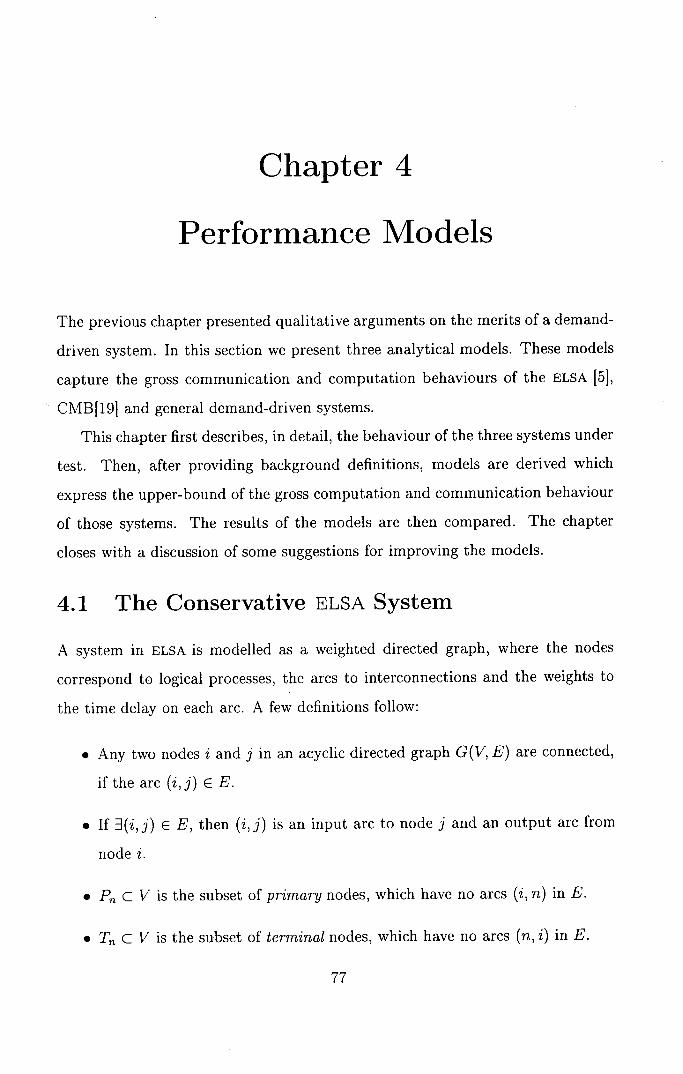
Chapter 4
Performance Models
The previous chapter presented qualitative arguments on the merits of a demand-
driven system. In this section we present three analytical models. These models
capture the gross communication and computation behaviours of the ELSA [5],
CMB[19] and general demand-driven systems.
This chapter first describes, in detail, the behaviour of the three systems under
test. Then, after providing background definitions, models are derived which
express the upper-bound of the gross computation and communication behaviour
of those systems. The results of the models are then compared. The chapter
closes with a discussion of some suggestions for improving the models.
4.1 The Conservative ELSA System
A system in ELSA is modelled as a weighted directed graph, where the nodes
correspond to logical processes, the arcs to interconnections and the weights to
the time delay on each arc. A few definitions follow:
• Any two nodes i and j in an acyclic directed graph G(V, E) are connected,
if the arc (i,j) E E.
• If 3 (Z', J) E E, then (Z', J') is an input arc to node j and an output arc from
node i.
• P, C V is the subset of primary nodes, which have no arcs (i, n) in E.
• T C V is the subset of terminal nodes, which have no arcs (n, i) in E.
77

. The set I = V - P - T of internal nodes.
Primary nodes place packets of information (or tuples) on arcs and terminal
nodes remove them from arcs. An internal node places tuples on its output arcs,
if and only if, it has removed a tuple from each of its input arcs. In its simplest
form, a tuple has three fields: V - state field, st and ed - the start and end times
for which the state field is valid. This has some similarities with the concept of
look-ahead in that the interval could be considered as an event at time st with a
look-ahead of ed-st. The difference is that while look-ahead states the minimum
time for which the state is valid, the end time (ed) states the time at which the
state becomes invalid. Associated with each input arc is a memory element which
stores the tuple while it is valid.
The system starts with an initialisation phase (Figure 4.1(a)). During this
phase the input memory elements of all the logical processes have their start and
end times both set to zero (the start of simulation time). The state need not be
set as it will be overwritten by an incoming tuple before being read. Also, each
logical process places a tuple on its output arc with the following information:
state (V) is set to whatever value is desired, the start time (st) is set to zero and
the end time set to 6, where 8 is the simulation time taken for a change in an
input value to affect the value of the output value (modelling the processing time
in the simulated system). This tuple indicates the initial state on the arcs. It is
safe to place this tuple on the arcs as the algorithm prevents any input to the
node from affecting the output state until the node's delay 6 has elapsed. This is
justified as no event at the inputs can cause an event at the output requiring a
start time less than J.
Once this initialisation phase is complete, the nodes are ready to start. A node
can only fire (generate an output event) when all its inputs have tuples whose
start time is different from their end time. As all the arcs have been initialised
with such tuples, as soon as they arrive at their destination, that node can fire.
(Figure 4.1(b) and 4.1(c))
The firing of a node has two parts; the creation and sending of the output
event (Figure 4.1(d), and the modification of the inputs to reflect the simulation
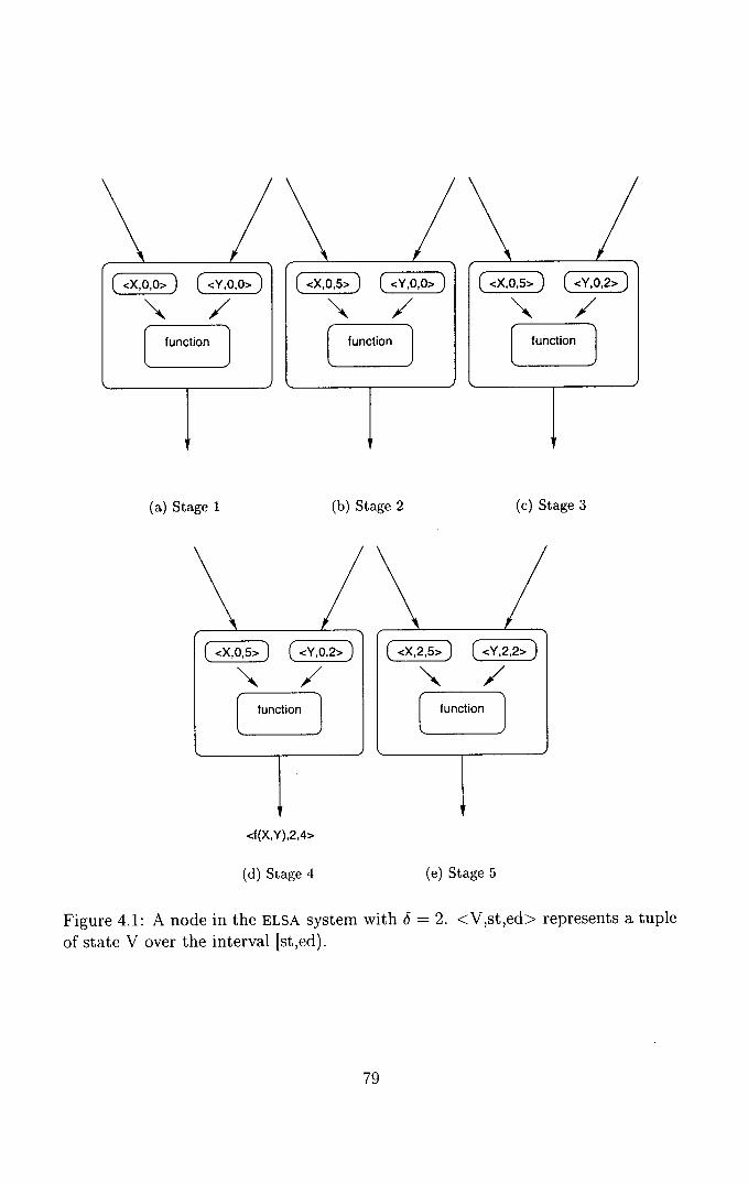
[,O,5>D (<v,o,o> J /
function
(a) Stage 1
(b) Stage 2
(c) Stage 3
_______J _______
/
/ [ function -
[function ]
<f(X,Y),2,4>
(d) Stage 4
(e) Stage 5
Figure 4.1: A node in the ELSA system with 6 = 2. <V,st,ed> represents a tuple of state V over the interval [st,ed).
79
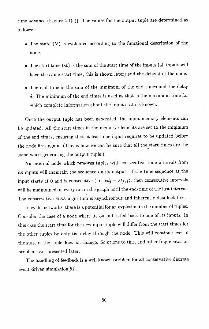
time advance (Figure 4.1(e)). The values for the output tuple are determined as
follows:
• The state (V) is evaluated according to the functional description of the
node.
• The start time (st) is the sum of the start time of the inputs (all inputs will
have the same start time, this is shown later) and the delay S of the node.
• The end time is the sum of the minimum of the end times and the delay
5. The minimum of the end times is used as that is the maximum time for
which complete information about the input state is known.
Once the output tuple has been generated, the input memory elements can
be updated. All the start times in the memory elements are set to the minimum
of the end times, ensuring that at least one input requires to be updated before
the node fires again. (This is how we can be sure that all the start times are the
same when generating the output tuple.)
An internal node which removes tuples with consecutive time intervals from
its inputs will maintain the sequence on its output. If the time sequence at the
input starts at 0 and is consecutive (i.e. ed3 = st +i), then consecutive intervals
will be maintained on every arc in the graph until the end-time of the last interval.
The conservative ELSA algorithm is asynchronous and inherently deadlock free.
In cyclic networks, there is a potential for an explosion in the number of tuples.
Consider the case of a node where its output is fed back to one of its inputs. In
this case the start time for the new input tuple will differ from the start times for
the other tuples by only the delay through the node. This will continue even if
the state of the tuple does not change. Solutions to this, and other fragmentation
problems are presented later.
The handling of feedback is a well known problem for all conservative discrete
event driven simulation(51].
Rml
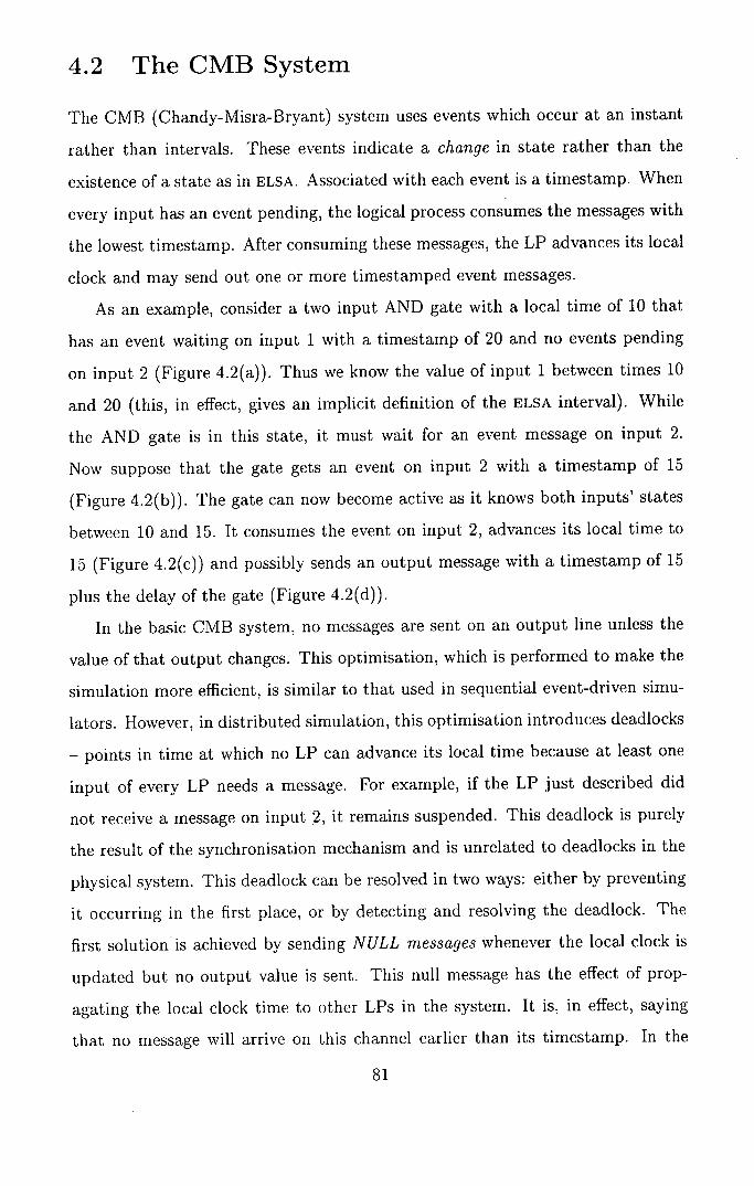
4.2 The CMB System
The CMB (Chandy-Misra-Bryant) system uses events which occur at an instant
rather than intervals. These events indicate a change in state rather than the
existence of a state as in ELSA. Associated with each event is a timestamp. When
every input has an event pending, the logical process consumes the messages with
the lowest timestamp. After consuming these messages, the LP advances its local
clock and may send out one or more timestamped event messages.
As an example, consider a two input AND gate with a local time of 10 that
has an event waiting on input 1 with a timestamp of 20 and no events pending
on input 2 (Figure 4.2(a)). Thus we know the value of input 1 between times 10
and 20 (this, in effect, gives an implicit definition of the ELSA interval). While
the AND gate is in this state, it must wait for an event message on input 2.
Now suppose that the gate gets an event on input 2 with a timestamp of 15
(Figure 4.2(b)). The gate can now become active as it knows both inputs' states
between 10 and 15. It consumes the event on input 2, advances its local time to
15 (Figure 4.2(c)) and possibly sends an output message with a timestamp of 15
plus the delay of the gate (Figure 4.2(d)).
In the basic CMB system, no messages are sent on an output line unless the
value of that output changes. This optimisation, which is performed to make the
simulation more efficient, is similar to that used in sequential event-driven simu-
lators. However, in distributed simulation, this optimisation introduces deadlocks
- points in time at which no LP can advance its local time because at least one
input of every LP needs a message. For example, if the LP just described did
not receive a message on input 2, it remains suspended. This deadlock is purely
the result of the synchronisation mechanism and is unrelated to deadlocks in the
physical system. This deadlock can be resolved in two ways: either by preventing
it occurring in the first place, or by detecting and resolving the deadlock. The
first solution is achieved by sending NULL messages whenever the local clock is
updated but no output value is sent. This null message has the effect of prop-
agating the local clock time to other LPs in the system. It is, in effect, saying
that no message will arrive on this channel earlier than its timestamp. In the
riii
(a) Stage 1 (b) Stage 2
C <E,20>j C_______
\/ r function
LT=15
<E3,17>
(c) Stage 3 (d) Stage 4
Figure 4.2: A node in the Chandy-Misra-Bryant (CMB) system with 8 = 2. <E,st> represents a tuple of event E at the timestamp st.
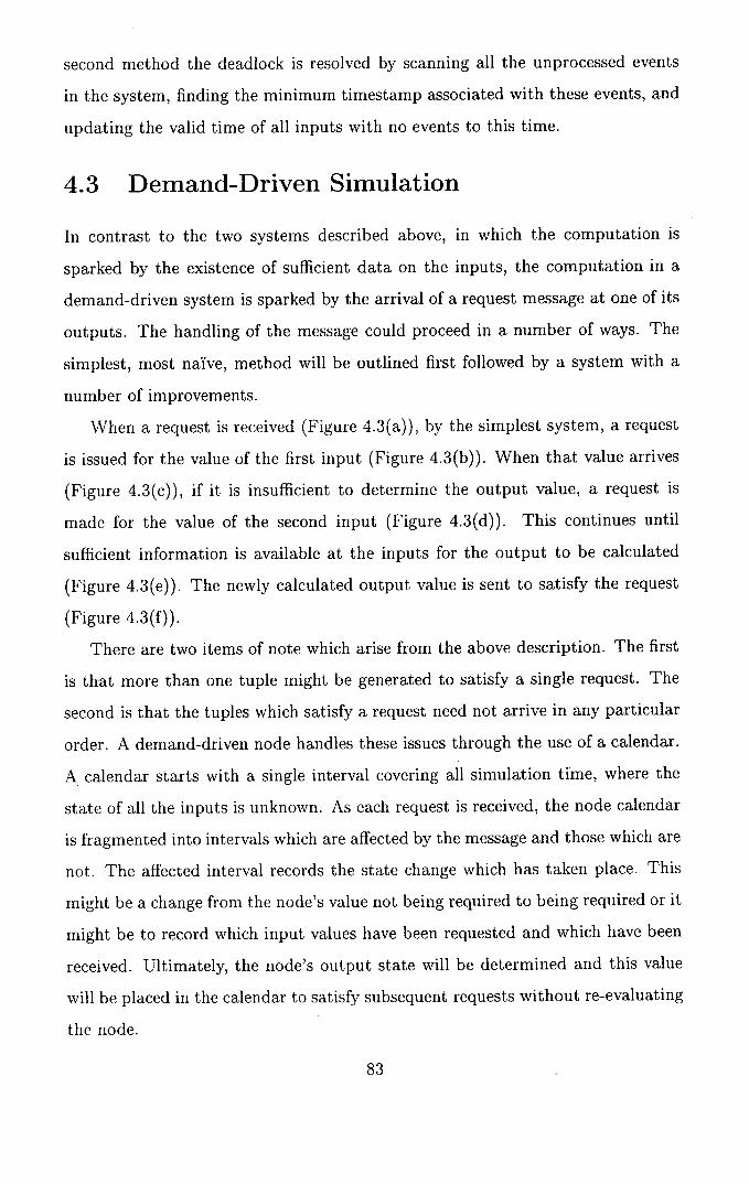
second method the deadlock is resolved by scanning all the unprocessed events
in the system, finding the minimum timestamp associated with these events, and
updating the valid time of all inputs with no events to this time.
4.3 Demand-Driven Simulation
In contrast to the two systems described above, in which the computation is
sparked by the existence of sufficient data on the inputs, the computation in a
demand-driven system is sparked by the arrival of a request message at one of its
outputs. The handling of the message could proceed in a number of ways. The
simplest, most naïve, method will be outlined first followed by a system with a
number of improvements.
When a request is received (Figure 4.3(a)), by the simplest system, a request
is issued for the value of the first input (Figure 4.3(b)). When that value arrives
(Figure 4.3(c)), if it is insufficient to determine the output value, a request is
made for the value of the second input (Figure 4.3(d)). This continues until
sufficient information is available at the inputs for the output to be calculated
(Figure 4.3(e)). The newly calculated output value is sent to satisfy the request
(Figure 4.3(f)).
There are two items of note which arise from the above description. The first
is that more than one tuple might be generated to satisfy a single request. The
second is that the tuples which satisfy a request need not arrive in any particular
order. A demand-driven node handles these issues through the use of a calendar.
A calendar starts with a single interval covering all simulation time, where the
state of all the inputs is unknown. As each request is received, the node calendar
is fragmented into intervals which are affected by the message and those which are
not. The affected interval records the state change which has taken place. This
might be a change from the node's value not being required to being required or it
might be to record which input values have been requested and which have been
received. Ultimately, the node's output state will be determined and this value
will be placed in the calendar to satisfy subsequent requests without re-evaluating
the node.
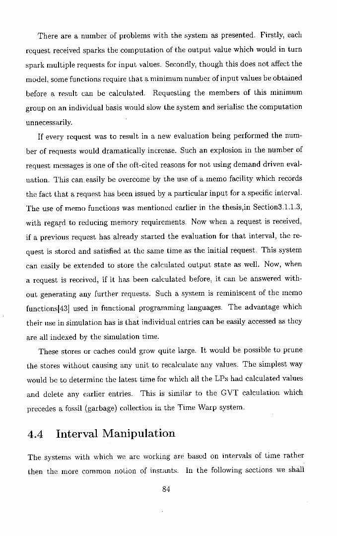
There are a number of problems with the system as presented. Firstly, each
request received sparks the computation of the output value which would in turn
spark multiple requests for input values. Secondly, though this does not affect the
model, some functions require that a minimum number of input values be obtained
before a result can be calculated. Requesting the members of this minimum
group on an individual basis would slow the system and serialise the computation
unnecessarily.
If every request was to result in a new evaluation being performed the num-
ber of requests would dramatically increase. Such an explosion in the number of
request messages is one of the oft-cited reasons for not using demand driven eval-
uation. This can, easily be overcome by the use of a memo facility which records
the fact that a request has been issued by a particular input for a specific interval.
The use of memo functions was mentioned earlier in the thesis,in Section3.1.1.3,
with regard to reducing memory requirements. Now when a request is received,
if a previous request has already started the evaluation for that interval, the re-
quest is stored and satisfied at the same time as the initial request. This system
can easily be extended to store the calculated output state as well. Now, when
a request is received, if it has been calculated before, it can be answered with-
out generating any further requests. Such a system is reminiscent of the memo
functions[43] used in functional programming languages. The advantage which
their use in simulation has is that individual entries can be easily accessed as they
are all indexed by the simulation time.
These stores or caches could grow quite large. It would be possible to prune
the stores without causing any unit to recalculate any values. The simplest way
would be to determine the latest time for which all the LPs had calculated values
and delete any earlier entries. This is similar to the GVT calculation which
precedes a fossil (garbage) collection in the Time Warp system.
4.4 Interval Manipulation
The systems with which we are working are based on intervals of time rather
then the more common notion of instants. In the following sections we shall
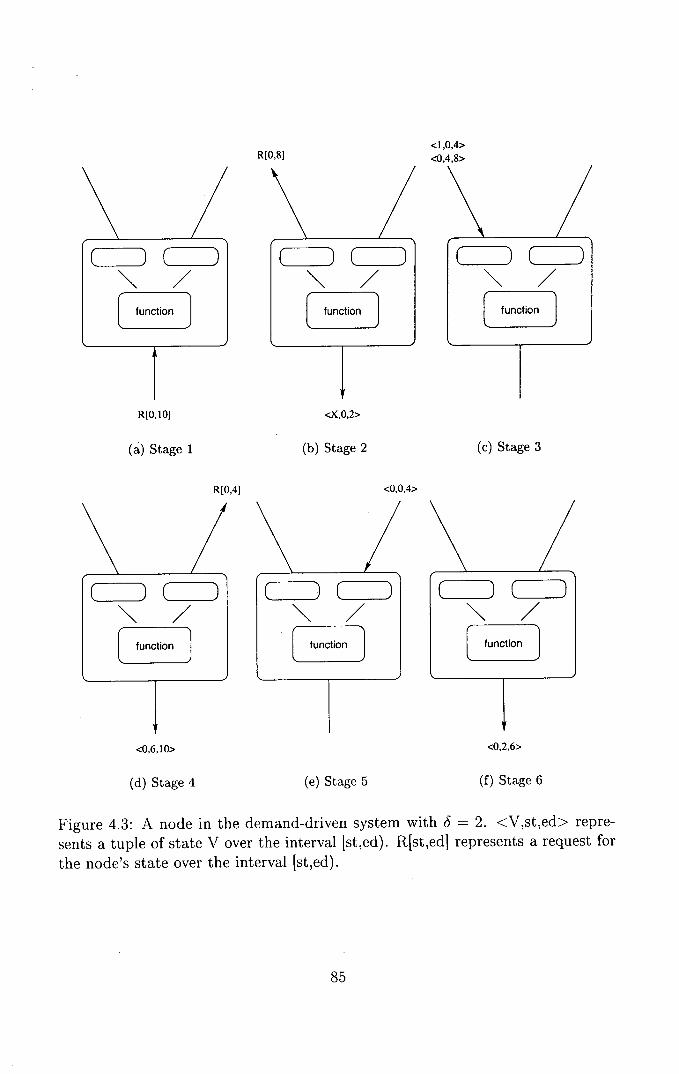
<1,0,4> R[0,8] <0,4,8>
cc_ /
[ctionj
[
[
R[0,10]
<X,0,2>
(a) Stage 1
(b) Stage 2
(c) Stage 3
R[0,4] <0,0,4>
c— c -
function
function
[
<0,6,10> <0,2,6>
(d) Stage 4
(e) Stage 5
(f) Stage 6
Figure 4.3: A node in the demand-driven system with 6 = 2. <V,st,ed> repre-sents a tuple of state V over the interval [st,ed). Rst,ed1 represents a request for the node's state over the interval Ist,ed).

define intervals and relations and operations upon intervals. Using the interval
system thus defined we will show how the ELSA and demand-driven systems would
perform and thus how the analytical models of their behaviour were created.
4.4.1 Definition and relations
An interval [a, b) covers all values, x, such that a < x < b. This definition rules
out instants such as [a, a) and intervals [4, 2) where a > b. For interval t, we shall
define the start time as t and the end time as t
From the definition above it is obvious that
[a,b)U[b,c) [a, c) (4.1)
Two intervals are said to overlap if, and only if, they have some interval in
common.
Overla (a b) = J [max(a,b),min(a,b)) iffmax(a,bj <min(a,b) undefined otherwise
(4.2)
Ingalls[44] uses a similar definition but uses closed intervals. The use of closed
intervals permits the existence of instants, i.e. [3,3], which are ruled out in our
definition of an interval as we explicitly require a state to exist for a non-zero
amount of time.
A stream is a set of intervals where no two intervals overlap. A complete
stream over [a, b) is a stream whose intervals are consecutive and which can,
through repeated applications of the identity expressed in Equation 4.1, be shown
to be equivalent to the interval [a, b).
4.4.2 ELSA nodes
A strict ELSA node can only determine the output time interval when all the
input intervals are known. The output interval is the interval which is common
to all the input intervals. If we consider a two input node (inputs A and B) then
the output intervals can be determined as follows:
of
Compare each interval in stream A with every interval in stream B to de-
termine if the two intervals overlap (using the definition in Equation 4.2).
If there is an overlap, then add it to the output stream.
Assuming that A and B are complete streams then D will be a complete
stream. In order to determine the output stream of an ELSA node, it is necessary
to apply one more function. This function, 5, will move the stream forward in
time to mimic the effect of the delay through the node. The S function takes a
time (t), which is the delay, and an interval (a). The S functions adds the value
of t to both the start and end times of the interval. For example, if the interval
is [5,10) and the value oft is 3, then the result of the function will be the interval
18,13).
So far we have shown how to calculate the section of the output stream which
is dependent on the input streams. The time between the start of the simulation
and the first result appearing at the output of the node still needs to be accounted
for. To do this we simple add another interval to the output stream. This is the
interval [0,t), where t is the delay through the node. This is safe to do as the
interval starting at time 0, the start of simulation time, will be advanced by the
S function, mentioned above, by t, and thus cannot affect the output over the
interval [04).
It is therefore simple, if numerically taxing, to determine the number of in-
tervals which will be sent down any given arc for an acyclic graph. Cyclic graphs
add more complexity as their input streams must be merged with their output
streams until a fixed point is reached but the basic operations are the same.
The above is a description of events which take place in an ELSA simulation.
It only lacks data and function evaluation for it to be a complete description.
While the above system will provide, not only the number of messages but the
exact intervals, it also shows that the number of messages in an ELSA system is
independent of the data being carried. This is not, as we shall see, true of either
CMB or the proposed demand-driven systems.
[:yl
4.5 Analytical Models
We assume that the system being modelled is represented by a directed graph,
G = (V, E), where V is the set of nodes and E is the set of arcs (i, i). On any one
input arc all the events occur at discrete times and no two events on the same
arc occur at the same time. The events which arise on any arc can therefore be
represented as the set of times at which the event is raised. It is possible from
the set of event instants to recreate the intervals used by ELSA. The output of
any node is some function of its inputs at that time.
We are not directly concerned about when an event occurs, merely if an event
occurs. The event set is therefore represented by the probability of an event
occurring at time t.
We shall first outline the rules of probability before showing how to determine
the amount of traffic in the system and then, finally, apply a work cost to calculate
the work done by the system.
4.5.1 The Rules of Probability
Rule 1: If the probability of an event A is p(A), then the probability that A does
not happen is:
p(not A) = 1 - p(A)
Rule 2: Two events are mutually exclusive if they cannot both occur together.
The probability that one or the other occurs is the sum of the separate probabil-
ities:
p(A or B) = p(A) + p(B)
Rule 3: Two events are independent if the outcome of the first has no effect
on the outcome of the second. The probability that two independent events will
occur is the product of the separate probabilities:
p(A and B) = p(A) x p(B)
Rule 4: This is an approximation that is often used in risk calculations. While
it is not used in the simple models which will be used as examples, it would make
•1s1
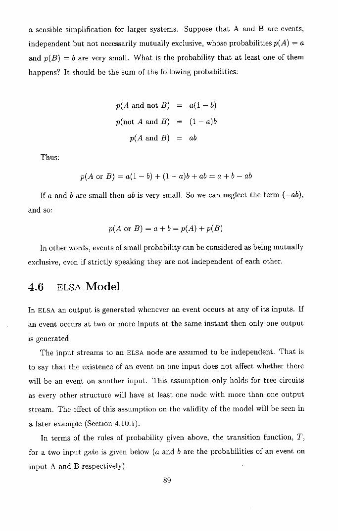
a sensible simplification for larger systems. Suppose that A and B are events,
independent but not necessarily mutually exclusive, whose probabilities p(A) = a
and p(B) = b are very small. What is the probability that at least one of them
happens? It should be the sum of the following probabilities:
p(A and not B) = a(1 - b)
p(not A and B) = (1 - a)b
p(A and B) = ab
Thus:
p(AorB)=a(1—b)+(1—a)b+ab=a+b—ab
If a and b are small then ab is very small. So we can neglect the term (—ab),
and so:
p(A or B) = a + b = p(A) + p(B)
In other words, events of small probability can be considered as being mutually
exclusive, even if strictly speaking they are not independent of each other.
4.6 ELSA Model
In ELSA an output is generated whenever an event occurs at any of its inputs. If
an event occurs at two or more inputs at the same instant then only one output
is generated.
The input streams to an ELSA node are assumed to be independent. That is
to say that the existence of an event on one input does not affect whether there
will be an event on another input. This assumption only holds for tree circuits
as every other structure will have at least one node with more than one output
stream. The effect of this assumption on the validity of the model will be seen in
a later example (Section 4.10.1).
In terms of the rules of probability given above, the transition function, T,
for a two input gate is given below (a and b are the probabilities of an event on
input A and B respectively).
T (a, b) = a + b - ab (4.3)
The transition function for three inputs is T(a, T(b, c)) T(T(a, b), c).
The probability of an event, p, multiplied by the run time of the system, n,
gives a measure of the number of events which flow down the arc.
4.7 CMB model
The model for a CMB system using NULL messages is the same as that presented
above for the ELSA system. This is because every message which arrives, whether
it is a NULL message or a data message, causes the generation of a new message.
This message is either an event message because the output value has changed or
it is a NULL message sent to indicate an increased local time.
In the version of the CMB system which uses a deadlock detection and res-
olution mechanism, an output event is only generated when an output changes
state. The model of the ELSA system is extended to allow for the probability that
the output value may change. We denote this probability by E.
The transition function remains the same but the input parameters are now
the product of the probability of an event, p, and the probability that that event
is different from the previous event, E. This gives the probability of an event
whose state is different from the- last event.
The derivation of the value of E on an output is dependent upon the function
which the node computes. Below we present the derivation assuming that an
exclusive-OR function is being computed.
The nature of the exclusive-OR function is that if both inputs change state
at the same time then the output will remain unchanged.
We therefore want the probability of either of the inputs changing state, but
not both. This can be shown by the Venn diagram in Figure 4.4.
The shaded area of Figure 4.4 can be expressed as follows:
PI E, +P2 E2 -2xP1 E1 P2E2
!1I
Figure 4.4: Venn diagram of A or B but not both
The probability of an event tends to the ratio of favourable events to trials,
as the number of trial increases. The equation for the probability of an output
event having a different state from the previous output is:
PEi 1122
- P1 E1 + P2E2 - P1 E1 P2 E2
As a new event is only dispatched along the output arcs if if is has a different
value from the previous event dispatched along the arcs, we can use the value of
E, defined above, to determine the number of real messages (as opposed to NULL
messages) send along output arcs.
4.8 Demand-Driven Model
The demand-driven model is substantially more complex than either the ELSA or
CMB models. This is due to the fact that the number of messages sent across
any arc can be dependent upon the number of messages sent across some different
arc. For example, the number of data messages being received on one arc can be
affected by the number and state of the data message being received on another
input.
The model is illustrated by a four port unit (Figure 4.5). Each port is bi-
directional and is capable of both sending and receiving messages. This is required
as each port must be able to send data messages and receive request messages or
vice versa.
91
Data in
Requests out
Node
Requests in
Data out
Figure 4.5: A sample node.
4.8.1 communication costs
We make use of information already calculated for the ELSA model when we calcu-
late the communications load for the demand driven approach. The ELSA model
provides the communication load when the data on each link is required 100% of
the time. With demand-driven simulation this is not the case. We shall use the
ELSA calculations when we start to determine the demand-driven data commu-
nications load.
Each arc can be given a weighting (W) which will indicate the percentage of
the time for which it is actually required. If a node has two or more output arcs
which means, in turn, that the node has two or more sources of requests, then
the effective amount of time for which the node is required to be active is some
function of the percentages of the request streams. By the same argument used
in Section 4.5.1, the function is T, the transition function.
The node will be active when one, or more, of the independent input arcs is
active. Therefore, the effective fraction of the run for which the node is active is
given by
W = T(X),X = jWjj : (i,j) E E}
92
We now need to determine the weighting on each link in turn W.
If the node is active for W, percent of the time then it must have, at least, one
link active for that time. Therefore the first input will have requests covering W2
percent. For convenience we shall order the n inputs to a node and label them
from 0 to n - 1. We shall denote the source of the arc as src(j).
T/Vi, src(0) = Wi
The percentage of request activity on the second and subsequent arcs is depen-
dent upon the function being evaluated at the node. There is a certain probability
that more data will be required, for node i, once the first request is satisfied, let
us call this M(, i ). The amount of request activity on the second input arc is
M(j) times the activity percentage of the first arc. The value M(, 2 ) is the prob-
ability that more data is required after both the first and second arcs have been
evaluated. This continues until all n of the input arcs have been evaluated. The
value of M(,) must be zero as there are no further sources of data left to be
interrogated. M(,o) is 0 for all primary inputs (as they must, by definition, know
their output without computation) and 1 otherwise.
i- i
T47isrc(j) = T47 H IVI(i,k)
k=O
This enables us to estimate what percentage of the time each arc will be active.
Now that we know how many messages will be transmitted on all the arcs if
they were active for all the simulation run, and the percentage of their activity,
we can determine the number of data message passed over each arc.
DCjj = Cjj x Wi,j
There only remains the number of request messages sent over each link to be
determined.
If there is only one output arc then the number of requests sent over the first
input arc is the same as the number of requests received from that output arc.
Should there be more than one output arc then the number of request messages
is some function of the incoming request streams.
93
The function is, once again, the transition function T. The parameters of the
function are based on the probability of a request message being received.
Ri,src(0) - T(X), X = {R 3 , : ( i, i) E E}
The model is completed with the generation of the probability of requests
on the remaining input arcs. Each arc, apart from the first one, gets a number
of requests based on the number of incoming messages on the previous arc. As
mentioned earlier, each arc has associated with it a probability, M. The number
of requests sent up the next input in turn is
,src(j) = M(,_1) (csrc(j_l)i)
The value Csrc(j_I),i is divided by n to get the probability of a data message
arriving.
4.8.2 Computation costs
The handling of a request message should require significantly less real time than
the handling of a data message. We denote by g the relative granularity of the
work being performed at a node. A granularity of 10 means that the node takes
10 times as long to process a data message as it does to process a request message.
Just as we noted in Section 3.1.1.1, data and request messages do not have the
same communication or computation requirements.
To obtain a measure of work performed in a data-driven system we sum the
work done at all of the nodes. The work performed at a node can be determined by
the number of output messages which need to be generated and granularity. Note
that this provides a relative measure and not an absolute statement of simulation
time.
To obtain a measure of work performed in a demand-driven system we deter-
mine the useful work performed in the same manner as the data-driven system.
We then need to add the number of request messages which need processing.
Again, this gives a relative measure, but it can be used in comparisons.
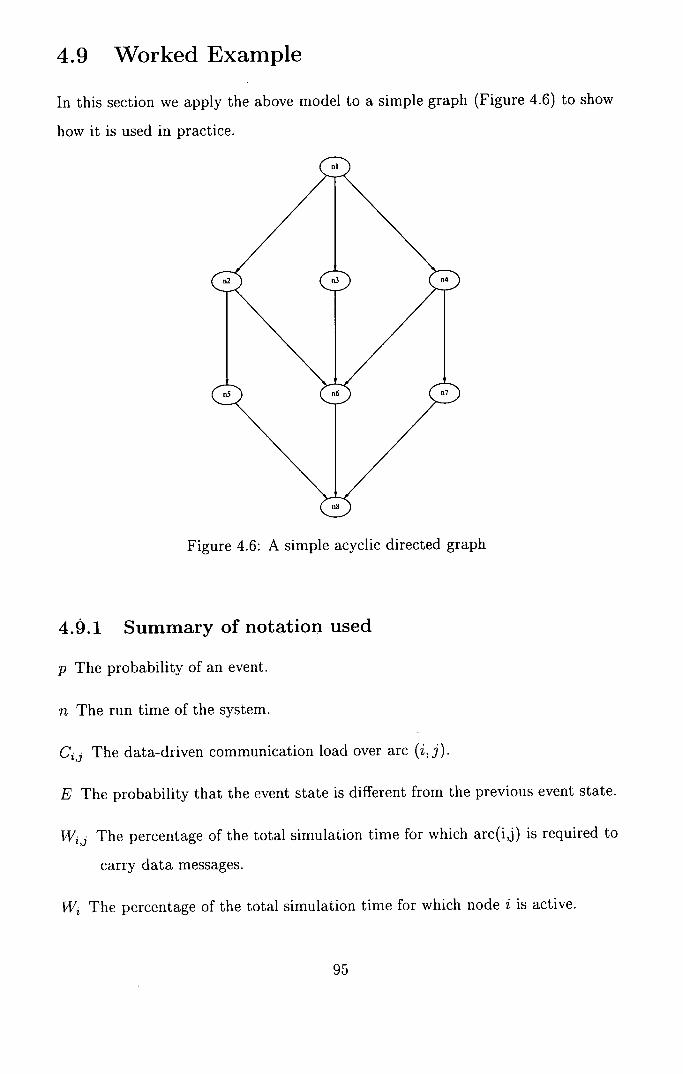
4.9 Worked Example
In this section we apply the above model to a simple graph (Figure 4.6) to show
how it is used in practice.
Figure 4.6: A simple acyclic directed graph
4.9.1 Summary of notation used
p The probability of an event.
n The run time of the system.
Cjj The data-driven communication load over arc (i, i).
E The probability that the event state is different from the previous event state.
Wjj The percentage of the total simulation time for which arc(i,j) is required to
carry data messages.
Wi The percentage of the total simulation time for which node i is active.
95
M(,k) The probability that more data will be required once request k of node i
is satisfied.
DC,3 The number of data messages passed over demand-driven arc (i, i).
Rj, i The probability of a request message on arc (j, i).
T(a, b) The transition function which, given the probability of independent, but
not mutually exclusive, events occuring on inputs a and b, can give the
probability of an event occuring on input a, or on input b or on both a and
g The relative granularity of productive work to request message handling.
4.9.2 ELSA data-driven model
For the data driven model we shall assume that the two parameters p and ii are
known. This leads to equations for the number of dta messages on the outputs
of nodes 1 . . . 4 as follows:
C1 , 2 = Ci , 3 = C1 , 4 = np
The data communication load from these nodes is the same as the data loads
into the nodes, hence:
C2 , 5 = C2 , 6 = C3 , 6 = C4 , 6 = C4 ,7 = np
A similar situation holds true for the communication outputs from nodes 5
and 7.
C5 ,8 = C7 ,8 = rip
The output of node 6 is a function of the inputs.
C26 C3 6 C4 ,6 \
((n ni C6 , 8 = T T ___L , , I n
= (p3 3p2 +3p)fl
This just leaves the data communications load for node 8.
Rol
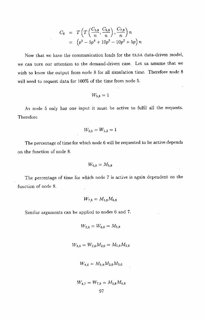
C8 = T(T(
C"8,—),'8" n Ti fli
= (P 5 -5 P4 + 1Op3 - 1Op2 + 5p)
Now that we have the communication loads for the ELSA data-driven model,
we can turn our attention to the demand-driven case. Let us assume that we
wish to know the output from node 8 for all simulation time. Therefore node 8
will need to request data for 100% of the time from node 5.
W 5 , 8 = 1
As node 5 only has one input it must be active to fulfil all the requests.
Therefore
= W 1 , 2 = 1
The percentage of time for which node 6 will be requested to be active depends
on the function of node 8.
T46,8 = 1 /5,8
The percentage of time for which node 7 is active is again dependent on the
function of node 8.
1/V7 ,8 =
Similar arguments can be applied to nodes 6 and 7.
1/V2 ,6 = 1'176,8 = 1'15,8
1/V3 , 6 = 1/V2 , 6 = M5,8 M2,6
1/V4 , 6
1474,7 = 1/V7 , 8 = M5,8 M6,8
97
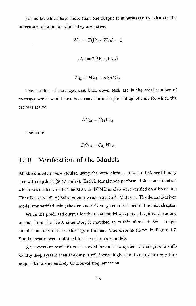
For nodes which have more than one output it is necessary to calculate the
percentage of time for which they are active.
W 1 , 2 = T(W 2 ,5 , T'V2 , 6 ) = 1
= T(VV, 6 , 1474,7)
1'V,3 = T'V6,3 = M5,8 M2,6
The number of messages sent back down each arc is the total number of
messages which would have been sent times the percentage of time for which the
arc was active.
DC1 , = C,3 W, 3
Therefore:
DC6 ,8 = C6 , 8 W 6 , 8
4.10 Verification of the Models
All three models were verified using the same circuit. It was a balanced binary
tree with depth 11 (2047 nodes). Each internal node performed the same function
which was exclusive-OR. The ELSA and CMB models were verified on a Breathing
Time Buckets (BTB)[841 simulator written at DRA, Malvern. The demand-driven
model was verified using the demand driven system described in the next chapter.
When the predicted output for the ELSA model was plotted against the actual
output from the DRA simulator, it matched to within about + 8%. Longer
simulation runs reduced this figure further. The error is shown in Figure 4.7.
Similar results were obtained for the other two models.
An important result from the model for an ELSA system is that given a suffi-
ciently deep system then the output will increasingly tend to an event every time
step. This is due entirely to interval fragmentation.
Error 0
0 0
0
0
0
o 00 0
00
0 0 CD
000 8 8
0 000 00
0000 0 00 0Z
00
0 000% 0 0 00
: 80 * 8 o
° 0
°000:ozo 08 ,00 0 /vo8
i0
00 kV
0
0 0
0o
0 00000 O
0 0
0 0
10
8
6
4 0
C)
2 0 C) 0 a-
0
-2
-4
0
0 0000 0
- 0 200 400 600 800 1000 Node number
Figure 4.7: Percentage error when comparing ELSA model to actual results from DRA simulator.
4.10.1 The effect of non-independent streams
As mentioned earlier, the models assume that the streams are independent. A
small case study using the gate level description of a 74LS283 adder[65] illustrates
the limitations of the ELSA model. This limitation propagates through the other
models as they are based, in part, on the ELSA model.
The parameters to the model were chosen arbitrarily:
. n, the run time, set to 1768.
• Values from the range , ,. . . assigned to the nine input probabilities.120
No two inputs had the same probability.
The measured and calculated results are compared in Figure 4.8. Note that,
while the model is a close representation in the early nodes (1.. . 9) the quality of
the model's predictions starts to decline in the next level (10. . . 28) until, by level
3, the model is assigning over 5 times as many messages to an arc as actually
pass across it. This over-estimate is the result of smaller over-estimates made in
the levels above and the lack of independence in the data streams.
450
400
350
300
250
200
150
tOO
50
cbsorved .-Prodicled
0 5 tO 15 20 25 30 35 40 45 Node Nurflbo,
Figure 4.8: Comparison of calculated and observed communications for 74LS283 adder.
Consider the data stream {5,10,15,20}. Its size is clearly 4. If this stream
is sent to both inputs of a two input gate then the output data stream, which
is basically the union of the input data streams, will also have a size of 4. If
however, one of the inputs had a delay of one unit then the output stream would
be {5,6,10,11,15,16,20,21} which has size 8. It is therefore plain that the diverse
paths taken from the data stream source to the destination gate can have a
dramatic effect on the size of the output data stream.
Consider node 29 of the adder (a node on the 3rd level of the network). Its
output stream is some function of its five input streams. The streams from nodes
10. . . 14 are themselves functions of streams.
n29= f(n io) n il , n 12 ,n13 ,n 14 )
n10 = f(n 2 )
nil = f(n i ,n4 )
n12 = f(ni,n3,n6)
n13 = f(n i ,n3 ,n5 ,n8 )
n14 = f(n 1 ,n3 ,n51 ri7 ,n9 )
As the above equations clearly show, the output from node n 1 is used four
times in determining the output stream from node 29. The delays of the interven-
100
ing nodes are chosen randomly from the range 11. . . 51. With four nodes choosing
from five discrete delays the probability that two or more of the nodes will choose
the same value is quite high (0.808)'
When the range of possible delays in increased, the observed number of mes-
sages at node 29 (and at other nodes) increases as predicted. The increase,
however, does not provide sufficient messages to meet the model's prediction.
These figures highlight the model's sensitivity to non-independent streams and
to small errors high in the circuit snowballing and swamping the count at deeper
levels.
4.10.2 Suggested improvements to the model
The greatest weakness of the model is that fact that it only considers local infor-
mation in determining the data or request activity of a node. As we saw in the
previous section, non-independent streams can cause the model to significantly
over-estimate the number of messages on any arc and thus the total amount of
work performed. This could be addressed in a number of different ways.
As we have seen in Section 4.4.2 it is possible, given the input intervals, to
determine exactly the levels of traffic across arcs in the ELSA system. As all the
models take as a base the data-driven level of traffic, then this might be used to
produce a tighter upper-bound on the message traffic, and thus on the amount
of work to be performed.
An alternative improvement would be to take into consideration the common
sources of the message traffic and also the various paths from source to the node
under consideration. If we have one stream taking two paths which had equal
delays then we could remove from consideration one of the streams, as it gives rise
to events which, as they occur at the same as those in the other stream, would
not cause an increase in the number transmitted. Currently the model assumes
independent streams and thus identical streams would be counted twice.
'The probability that two or more nodes will choose the same value is 1 minus the probability of all the nodes choosing different values. As there are 54 possible orderings of which 5 x 4 x 3 x 2 = 120 are unique, the number of orderings in which two or more nodes have the same delay is 0.808
101
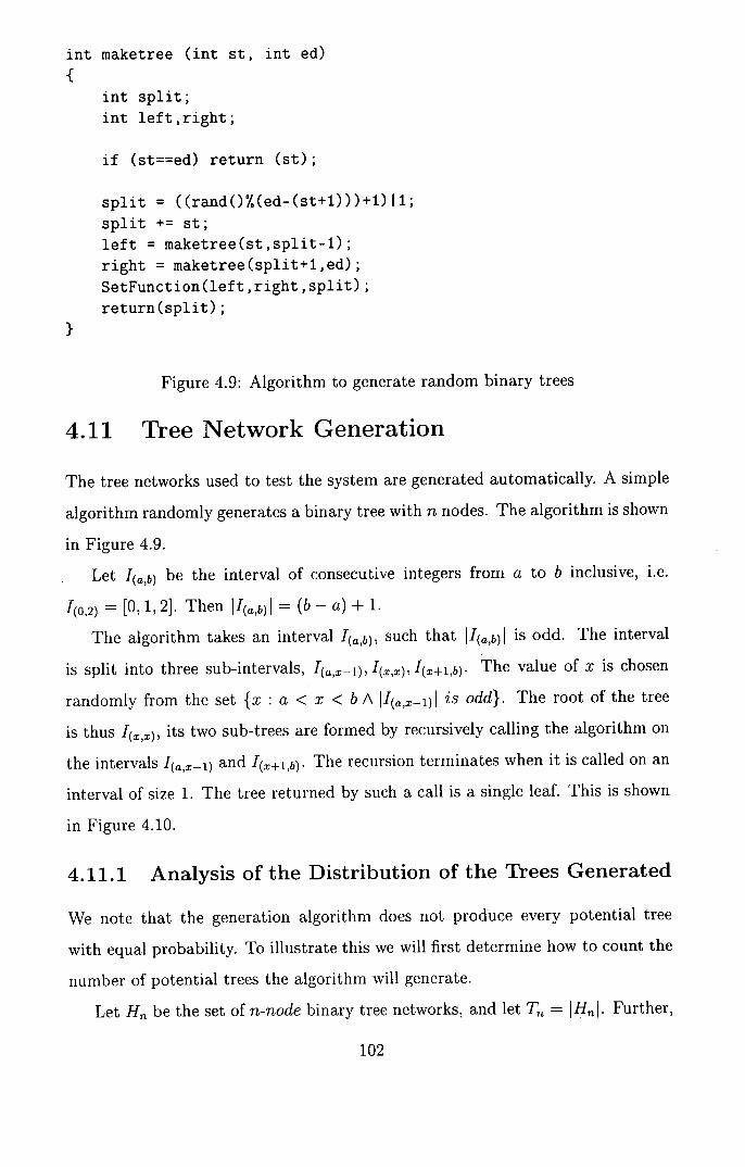
mt maketree (mt st, mt ed) {
mt split; mt left,right;
if (st==ed) return (st);
split = ((randO °h(ed-(st+1)))+1) Ii; split += st; left = maketree(st,split-1); right = maketree(split+1,ed); SetFunction(left ,right ,split); return (split)
}
Figure 4.9: Algorithm to generate random binary trees
4.11 Tree Network Generation
The tree networks used to test the system are generated automatically. A simple
algorithm randomly generates a binary tree with n nodes. The algorithm is shown
in Figure 4.9.
Let I(a,b) be the interval of consecutive integers from a to b inclusive, i.e.
1(0,2) = [0,1,2]. Then 11(a,b) I = (b - a) + 1.
The algorithm takes an interval I(a,b), such that II(a,b)l is odd. The interval
is split into three sub-intervals, '(ax—I), I(x,x), '(x+l,b) The value of x is chosen
randomly from the set {x : a < x < b A I(a,x-1)j is odd}. The root of the tree
is thus I(X,X), its two sub-trees are formed by recursively calling the algorithm on
the intervals I(a,xI) and '(x+1,b) The recursion terminates when it is called on an
interval of size 1. The tree returned by such a call is a single leaf. This is shown
in Figure 4.10.
4.11.1 Analysis of the Distribution of the Trees Generated
We note that the generation algorithm does not produce every potential tree
with equal probability. To illustrate this we will first determine how to count the
number of potential trees the algorithm will generate.
Let H,, be the set of n-node binary tree networks, and let T = IHII . Further,
102

let HL,R be the set of binary tree networks with L nodes in the left sub-tree and
R nodes in the right. Let TL,R = HL,Rl. As the sub-trees on the left and right of
the root node are independent the total number of possible trees is the product
of the number of sub-trees on the left and right.
TL,R = TLTR
Further, as the left and right sub-trees could be swapped, it is clear that
TL,R TR,L.
In general, we have the following recurrence relation for T. It is defined in
terms of the number of sub-trees generated by splitting the n nodes into sub-trees
of x and n - x - 1 nodes, where x ranges across the odd integers from 1 to m - 2
inclusive. fl-i
T =
The base case is T1 = 1. This is a single node with no children or parents. As
the number of nodes in a binary tree is always odd the next case is T3 = 1. This
represents a root with a leaf on both its sub-trees. The next case is T5 .
T5 = T1 , 3 +T3 , 1 = T1 T3 +T3T1 = 2
Values of T for small n are given in Table 4.1. It can be seen that T grows
rapidly; for networks of only 29 nodes, there are over 2 million different potential
trees that can be generated.
Now that we are able to count the number of trees with a given structure, we
will show that the distribution of generated trees is non-uniform. Consider the
generation of an 11 node tree. The number of tree with 11 nodes is given by:
T11 = T1 ,9 + T3 , 7 + T5 , 5 + T7 , 3 + T9 , 1
The above algorithm would generate a tree corresponding to one of the terms
above with equal probability of 1 . It should be noted, however, that T1 ,9 = T9 , 1 =
14 and T3 , 7 = T7 , 3 = 5 while T5 , 5 = 4. There are thus many more networks of type
H1 , 9 or H9 , 1 than of the other possible types. In effect, the algorithm is biased
towards producing balanced trees.
103
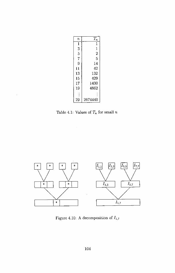
n T. 1 1 3 1 5 2 7 5 9 14
11 42 13 132 15 429 17 1430 19 4862
29 2674440
Table 4.1: Values of T for small n
Figure 4.10: A decomposition of Ii ,-,
104
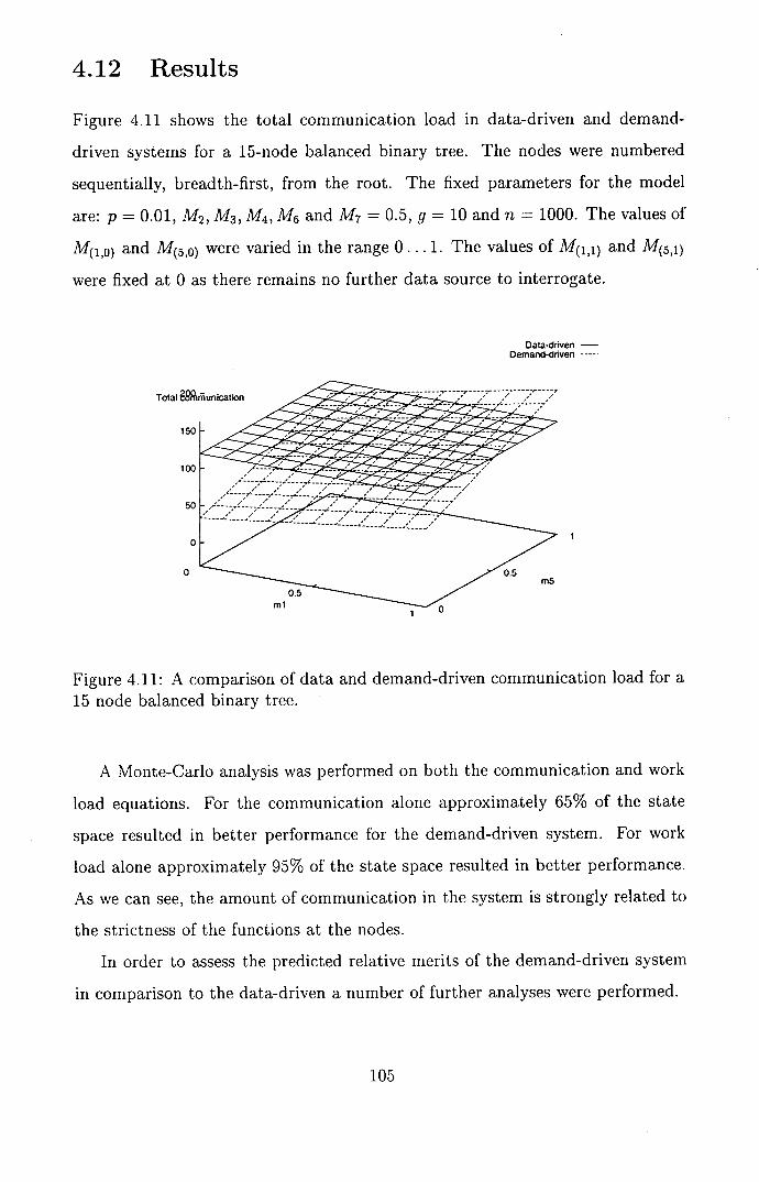
4.12 Results
Figure 4.11 shows the total communication load in data-driven and demand-
driven systems for a 15-node balanced binary tree. The nodes were numbered
sequentially, breadth-first, from the root. The fixed parameters for the model
are: p = 0.01, M2 , N!3 , M4 , NI6 and M7 = 0.5, g = 10 and n = 1000. The values of
M( i , o ) and M( 5 ,o ) were varied in the range 0. . . 1. The values of M( i , 1 ) and M(5,1)
were fixed at 0 as there remains no further data source to interrogate.
Data-driven - Demand-driven
Total
150
100
50
0
0
1
Figure 4.11: A comparison of data and demand-driven communication load for a 15 node balanced binary tree.
A Monte-Carlo analysis was performed on both the communication and work
load equations. For the communication alone approximately 65% of the state
space resulted in better performance for the demand-driven system. For work
load alone approximately 95% of the state space resulted in better performance.
As we can see, the amount of communication in the system is strongly related to
the strictness of the functions at the nodes.
In order to assess the predicted relative merits of the demand-driven system
in comparison to the data-driven a number of further analyses were performed.
105
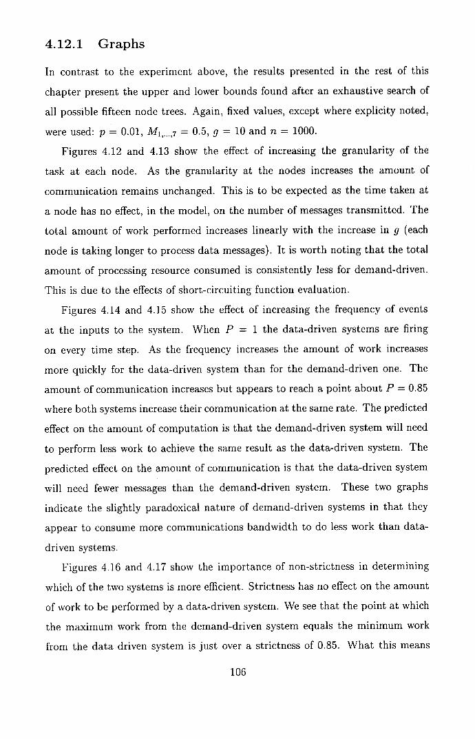
4.12.1 Graphs
In contrast to the experiment above, the results presented in the rest of this
chapter present the upper and lower bounds found after an exhaustive search of
all possible fifteen node trees. Again, fixed values, except where explicity noted,
were used: p = 0.01, M1 ,.,7 = 0.5, g = 10 and n = 1000.
Figures 4.12 and 4.13 show the effect of increasing the granularity of the
task at each node. As the granularity at the nodes increases the amount of
communication remains unchanged. This is to be expected as the time taken at
a node has no effect, in the model, on the number of messages transmitted. The
total amount of work performed increases linearly with the increase in g (each
node is taking longer to process data messages). It is worth noting that the total
amount of processing resource consumed is consistently less for demand-driven.
This is due to the effects of short-circuiting function evaluation.
Figures 4.14 and 4.15 show the effect of increasing the frequency of events
at the inputs to the system. When P = 1 the data-driven systems are firing
on every time step. As the frequency increases the amount of work increases
more quickly for the data-driven system than for the demand-driven one. The
amount of communication increases but appears to reach a point about P = 0.85
where both systems increase their communication at the same rate. The predicted
effect on the amount of computation is that the demand-driven system will need
to perform less work to achieve the same result as the data-driven system. The
predicted effect on the amount of communication is that the data-driven system
will need fewer messages than the demand-driven system. These two graphs
indicate the slightly paradoxical nature of demand-driven systems in that they
appear to consume more communications bandwidth to do less work than data-
driven systems.
Figures 4.16 and 4.17 show the importance of non-strictness in determining
which of the two systems is more efficient. Strictness has no effect on the amount
of work to be performed by a data-driven system. We see that the point at which
the maximum work from the demand-driven system equals the minimum work
from the data driven system is just over a strictness of 0.85. What this means
10111
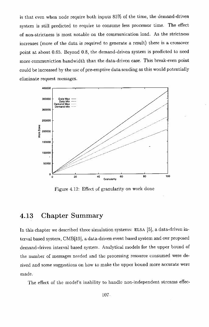
is that even when node require both inputs 85% of the time, the demand-driven
system is still predicted to require to consume less processor time. The effect
of non-strictness is most notable on the communication load. As the strictness
increases (more of the data is required to generate a result) there is a crossover
point at about 0.65. Beyond 0.8, the demand-driven system is predicted to need
more communiction bandwidth than the data-driven case. This break-even point
could be increased by the use of pre-emptive data sending as this would potentially
eliminate request messages.
400000
350000
300000
250000
a, C
200000
150000
100000
50000
0 0 20 40 60 80 100
Granularity
Figure 4.12: Effect of granularity on work done
4.13 Chapter Summary
In this chapter we described three simulation systems: ELSA [5], a data-driven in-
terval based system, CM13[19], a data-driven event based system and our proposed
demand-driven interval based system. Analytical models for the upper bound of
the number of messages needed and the processing resource consumed were de-
rived and some suggestions on how to make the upper bound more accurate were
The effect of the model's inability to handle non-independent streams effec-
107
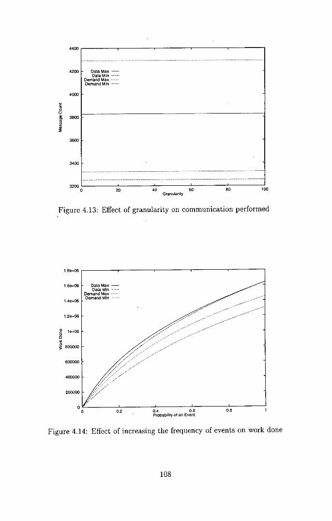
4400
4200
4000
C 0 0 0
, 3800
(a w
3600
3400
VI
0 20 40 60 80 100 Granularity
Figure 4.13: Effect of granularity on communication performed
1.8e+06
1.6e+06
1.4e+06
1.2e+06
le+06 0
800000
600000
400000
200000
- Data Max - Data Mm
Demand Max .....
Demand Mm ...........
. .
. .
............... .....
. .........
. .. ................
0 0.2 0.4 0.6 0.8 Probability of an Event
Figure 4.14: Effect of increasing the frequency of events on work done
- Data Max - Data Mm- -----
Demand Max .....
Demand Mm...........
IIIINI
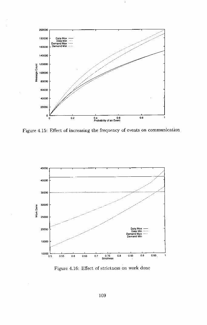
200000
180000
160000
140000
120000 r 0 0
, 100000
(a a,
80000
60000
40000
20000
n
/V
0 0.2 0.4 0.6 0.8 Probability of an Event
Figure 4.15: Effect of increasing the frequency of events on communication
45000
40000
35000
a, 30000 C 0 0
0
25000
20000
15000
10000 1
LL
0.5 0.55 0.6 0.65 0.7 0.75 0.8 0.85 0.9 0.95 Strictness
Figure 4.16: Effect of strictness on work done
109
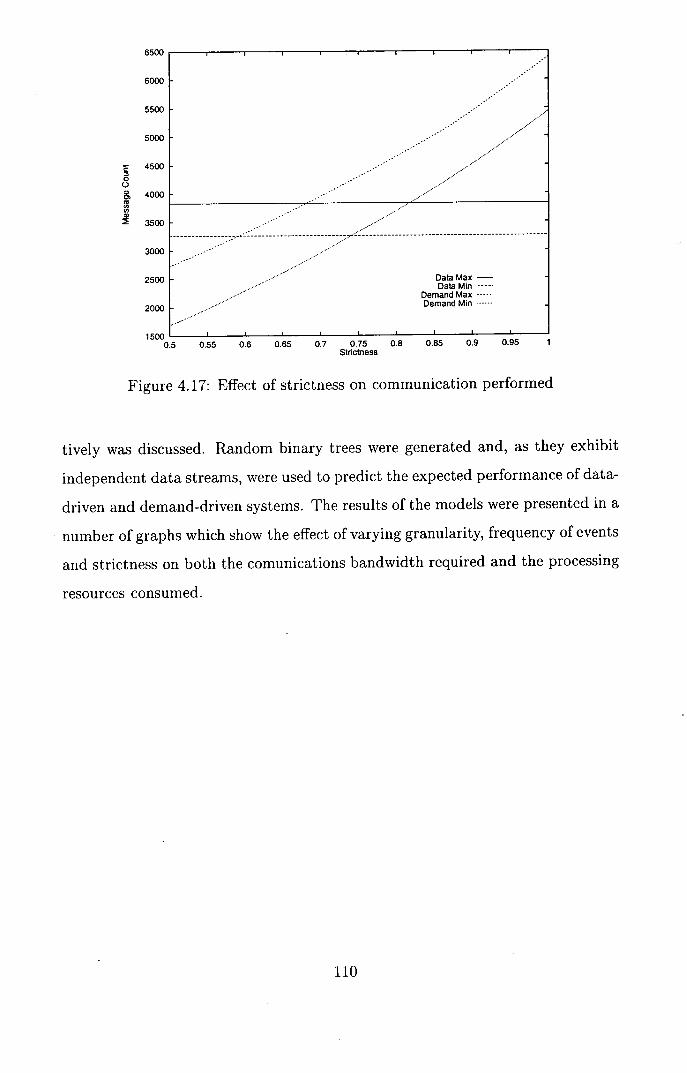
6500
6000
5500
5000
4500 = 0 0
4000 G0
3500
3000
2500
2000
i cnn
Data Max - Data Mm
Demand Max .....
Demand Mm
• 0.5 0.55 0.6 0.65 0.7 0.75 0.8 0.85 0.9 0.95 Strictness
Figure 4.17: Effect of strictness on communication performed
tively was discussed. Random binary trees were generated and, as they exhibit
independent data streams, were used to predict the expected performance of data-
driven and demand-driven systems. The results of the models were presented in a
number of graphs which show the effect of varying granularity, frequency of events
and strictness on both the comunications bandwidth required and the processing
resources consumed.
110
Chapter 5
Experimental Results
The model described previously is only able to give estimates of the total amount
of computation or communication 1 performed by any node. It cannot provide
information relating to the distribution of work through time nor can it give any
indication of how increasing the resources can affect the performance.
In this chapter a number of different circuits are used to examine the dy-
namic nature of the simulation and, in particular, to focus on the parallelism and
performance which is available as the computing resource increases.
5.1 The Test-bed
All the experimental results have been obtained from running the simulations
within the controlled environment of a multiprocessor simulator. The reason
for doing this was to have as much control of the "machine" as possible which
enabled the results to be obtained without interference from other users or being
dependent on factors such as caching or network load. The ultimate aim was to
provide reproducible results. In order for these results to have any validity it is,
of course, necessary to show that the simulator is a fair representation of a real
system. This is shown later.
As the tests are performed within the test-bed it is necessary to define our
concepts of simulation time and how it maps onto "real" time. Consider a circuit
being simulated on the multiprocessor test bed. Simulation time relates to time as
it is understood by the system being simulated - in this case, the circuit. System
1 J11 future, the term work shall be used to mean either computation or communication.
111

time relates to the time of the test bed - this is the time used as real time.
The description of the test-bed has two parts: the micro model (how the
processor functions) and the macro model (how the micro models are connected).
5.1.1 The Micro Model
The micro model describes a processor-memory pair. The memory is strictly local
to the processor and there is no concept of global or shared memory. Nor is there
any concept of a shared, or global, clock.
The micro model is designed as a reactive system. A reactive system is one
where the units remain in some quiescent state until activated by a message or
signal. Some computation is then performed followed by zero or more messages
being sent to other units.
The messages which arrive at a processor are typed. The type determines
whether the body of the message contains data to be processed or a demand for
data'. The amount of time spent handling the message is dependent on its type
and the number of intervals to which it is applied. The complete evaluation of a
function for any time interval will require a number of messages to be processed.
When the node is idle (not processing any message) it waits until a message
arrives and then starts to handle that mesage. Should another message arrive
while the node is handling the first message, the arriving message waits in a
queue until the processor is idle once more. Messages are handled in the order in
which they arrive.
The handling of a message consists of updating the local state of the affected
process (the processor can host a number of processes) and sending the resultant
output messages, if any.
5.1.1.1 Message Handling
Each process maintains a separate state space which defines the state of that
process throughout the simulation time. A process can be at different states in
simulation time at any instant of system time.
'The number of such types could be increased to provide for a range of control messages. A use for such messages is presented later.
112
When a message is received the interval covered by the incoming message is
extracted from the state space. Should the incoming interval start or end in the
middle of an interval in the state space then that interval is split into two (the
part not affected by the incoming message and the part which is affected). Once
the affected portion of the state space is extracted the incoming message is then
applied to each interval in turn. What action is performed depends on the state
of extracted interval and the type of message received.
Demand Message:
When a demand message is applied to an interval, one of three actions can
occur:
If the state of the output for that interval is known then the demand can be
satisfied immediately. The output value is bundled into a message which is
sent to the process which initiated the demand.
If the state of the output for that interval is not known, but data to calculate
that state has been demanded, then the incoming demand is added to the
list of currently outstanding demands. It will be satisfied as soon as the
interval has a value.
If the state of the output for that interval is not known, and no earlier
demands have been made, then the incoming demand is put in a list of
outstanding demands and one or more demand is issued to the nodes whose
data is required to calculate the value of that interval.
Data Message:
When a data message is applied to an interval, one of two actions can occur:
If there is sufficient data available for the value of the interval to be deter-
mined, then all the outstanding demands (and there must be at least one)
are satisfied and the output value is stored.
Should there not yet be sufficient data available, then the incoming data
value is applied to the function for that interval and a demand for further
113
data is sent to the appropriate node. The interval state is thus the partially
evaluated result of the function. This enables short-circuit evaluation.
5.1.2 The Macro Model
The macro model describes how the final parallel resource is constructed and
gives the characteristics of the communication links.
The communication graph assumes that any processor can send data to any
other processor without interrupting the processing on a third, intermediate, pro-
cessor. There are three times associated with communications. The first is the
transport time; this is the time taken for a message to move through the network
from the source to the destination. The second and third times relate to the
processor work required to move the message to and from the processor into the
communications net. If a message is being sent to another process on the same
processor, this cost still applies.
Messages are queued at the destination in the order in which they arrive.
Should two or more messages arrive at the same time, then they are queued in
an arbitrary order.
In all of the experiments below, the nodes were scattered randomly across
the processors. This was done to try and eliminate either method gaining an
advantage from a more favourable distribution. For any individual experiment,
both the data and the demand driven methods were tested using the same random
distribution.
5.1.3 Test-bed Input/Output
Input and output is handled by special nodes which behave in a similar manner
to all the other nodes being simulated. The input nodes can be considered as
functions whose state is known for all simulation time, while the output nodes
are functions with one input which merely store the incoming data.
114

5.1.4 Model Output
As the simulation system is itself being run in a controlled environment it is
possible to take whatever measures are desired without affecting the system being
studied: this is one reason for using such an enviroment.
The output trace concentrates on the behaviour of the processors'. The pro-
cessor is constrained to be in one of four states and to start the simulation in
the idle state. Whenever a processor changes state that information is written to
the trace file and that state is known to persist until another state change event
occurs. Extra information is written to the trace file depending upon what state
the processor is entering. The exception to the above is the Mark event. This
event is used to record any information which is deemed relevant but does not
alter the state of the processor.
The states are given below:
idle: the processor is waiting for a message to arrive.
send: the processor is currently copying one or more messages onto the commu-
nications network.
recv: the processor is copying one message from the communications network.
task: the processor is occupied with internal processing and updating local sys-
tem state.
5.2 Increasing confidence in the veracity of the simulator
As mentioned earlier, when using a simulator, it is necessary to obtain evidence
that the simulator is, in fact, a reasonable representation of a real machine. The
method which was used to obtain such supporting evidence is in three parts:
1. Obtain values from a real machine for the parameters of the simulator.
3 The trace format is very similar to that used in PICL.
115

Obtain results for running the same circuit on both the real and the simu-
lated machines.
Compare the two results
5.2.1 The gentle art of Ping-Pong
The time taken to send a message from one process to another can be measured
by "bouncing" a message from one process off another process. By recording the
time taken by the message to travel to the other process and back again, and
assuming that the journey times are symmetrical, it is possible to determine the
time taken for the message to travel half the distance. It is reasonable to suppose
that the longer the message, then the more time it will take to transmit trough
the network and, as such, the measures are taken for a range of message lengths.
Two different graphs are presented below. The first (Figure 5.1) is for a multi-user
machine (the specification of the machine is in Table 5.1).
Machine ]_________ Attributes
Make Sun Calvay Model SS10
Memory 240M Purpose Staff compute and Xterm server
Make Sun Balta Model SS1+
Memory 11M Purpose Small desktop workstation
Table 5.1: Specification of test machines
Both graphs exhibit a similar linear trend. The graph for Calvay (Figure 5.1)
also shows one of the problems inherent in trying to take performance measures
on a multi-user machine, namely that the process is sharing the machine with
many others, all of which are making demands on the processor. As such the
times taken on Calvay can vary quite significantly, though, by taking sufficient
results, a trend starts to appear. The graph for Balta (Figure 5.2) shows the
linear trend much more clearly.
116
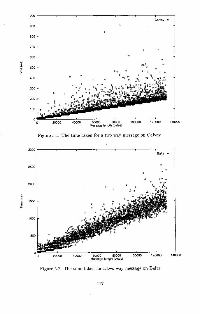
1000
900
800
700
600
C,)
E 500
E I-
400
300
200
100
0 0 20000 40000 60000 80000 100000 120000 140000
Message length (bytes)
Figure 5.1: The time taken for a two way message on Calvay
3000
2500
2000
0
E 'a;- 1500 E F-
1000
500
A
0 20000 40000 60000 80000 100000 120000 140000 Message length (bytes)
Figure 5.2: The time taken for a two way message on Balta
117
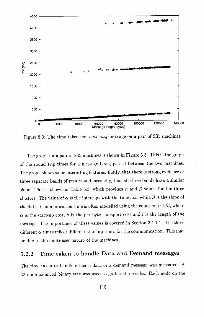
4500
4000
3500
3000
2500 E a) E
2000
1500
1000
500
0 0
0 o
000 • 0 00
400 ON&
20000 40000 60000 80000 100000 120000 140000 Message length (bytes)
Figure 5.3: The time taken for a two way message on a pair of SS5 machines
The graph for a pair of SS5 machines is shown in Figure 5.3. This is the graph
of the round trip times for a message being passed between the two machines.
The graph shows some interesting features: firstly, that there is strong evidence of
three separate bands of results and, secondly, that all three bands have a similar
slope. This is shown in Table 5.3, which provides a and 0 values for the three
clusters. The value of a is the intercept with the time axis while 0 is the slope of
the data. Communication time is often modelled using the equation a + 01, where
a is the start-up cost, 0 is the per byte transport cost and 1 is the length of the
message. The importance of these values is covered in Section 3.1.1.1. The three
different a times reflect different start-up times for the communication. This may
be due to the multi-user nature of the machines.
5.2.2 Time taken to handle Data and Demand messages
The time taken to handle either a data or a demand message was measured. A
32 node balanced binary tree was used to gather the results. Each node on the
118
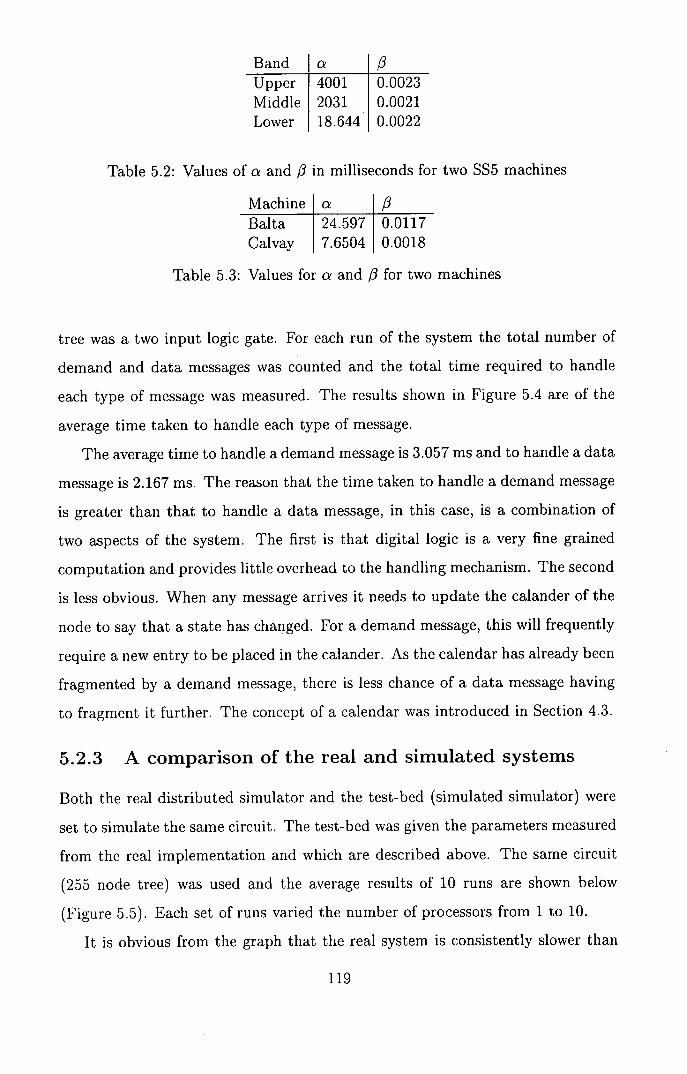
Band a /3 Upper 4001 0.0023 Middle 2031 0.0021 Lower 18.644 0.0022
Table 5.2: Values of a and 0 in milliseconds for two SS5 machines
Machine a 10 Balta 24.597 0.0117 Calvay 7.6504 0.0018
Table 5.3: Values for a and /3 for two machines
tree was a two input logic gate. For each run of the system the total number of
demand and data messages was counted and the total time required to handle
each type of message was measured. The results shown in Figure 5.4 are of the
average time taken to handle each type of message.
The average time to handle a demand message is 3.057 ms and to handle a data
message is 2.167 ms. The reason that the time taken to handle a demand message
is greater than that to handle a data message, in this case, is a combination of
two aspects of the system. The first is that digital logic is a very fine grained
computation and provides little overhead to the handling mechanism. The second
is less obvious. When any message arrives it needs to update the calander of the
node to say that a state has changed. For a demand message, this will frequently
require a new entry to be placed in the calander. As the calendar has already been
fragmented by a demand message, there is less chance of a data message having
to fragment it further. The concept of a calendar was introduced in Section 4.3.
5.2.3 A comparison of the real and simulated systems
Both the real distributed simulator and the test-bed (simulated simulator) were
set to simulate the same circuit. The test-bed was given the parameters measured
from the real implementation and which are described above. The same circuit
(255 node tree) was used and the average results of 10 runs are shown below
(Figure 5.5). Each set of runs varied the number of processors from 1 to 10.
It is obvious from the graph that the real system is consistently slower than
119
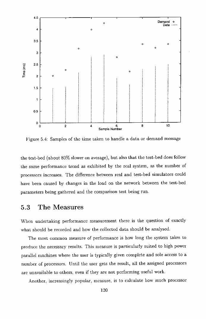
4.
4
3.5 0 0
0
3 0
2.5 E
0 0
E
2- 0
1.5 -
0.5
0
0 2 4 6 8 10 Sample Number
Figure 5.4: Samples of the time taken to handle a data or demand message
the test-bed (about 80% slower on average), but also that the test-bed does follow
the same performance trend as exhibited by the real system, as the number of
processors increases. The difference between real and test-bed simulators could
have been caused by changes in the load on the network between the test-bed
parameters being gathered and the comparison test being run.
5.3 The Measures
When undertaking performance measurement there is the question of exactly
what should be recorded and how the collected data should be analysed.
The most common measure of performance is how long the system takes to
produce the necessary results. This measure is particularly suited to high power
parallel machines where the user is typically given complete and sole access to a
number of processors. Until the user gets the result, all the assigned processors
are unavailable to others, even if they are not performing useful work.
Another, increasingly popular, measure, is to calculate how much processor
120
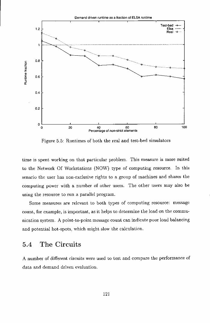
Demand driven runtime as a fraction of ELSA runtime
1.2
0.8 0
0
a, 0.6
C D
0.4
0.2
0 0
Test-bed -9---
Elsa ----- - Real -0--
0
20 40 60 80 100 Percentage of non-strict elements
Figure 5.5: Runtimes of both the real and test-bed simulators
time is spent working on that particular problem. This measure is more suited
to the Network Of Workstations (NOW) type of computing resource. In this
senario the user has non-exclusive rights to a group of machines and shares the
computing power with a number of other users. The other users may also be
using the resource to run a parallel program.
Some measures are relevant to both types of computing resource: message
count, for example, is important, as it helps to determine the load on the commu-
nication system. A point-to-point message count can indicate poor load balancing
and potential hot-spots, which might slow the calculation.
5.4 The Circuits
A number of different circuits were used to test and compare the performance of
data and demand driven evaluation.
121
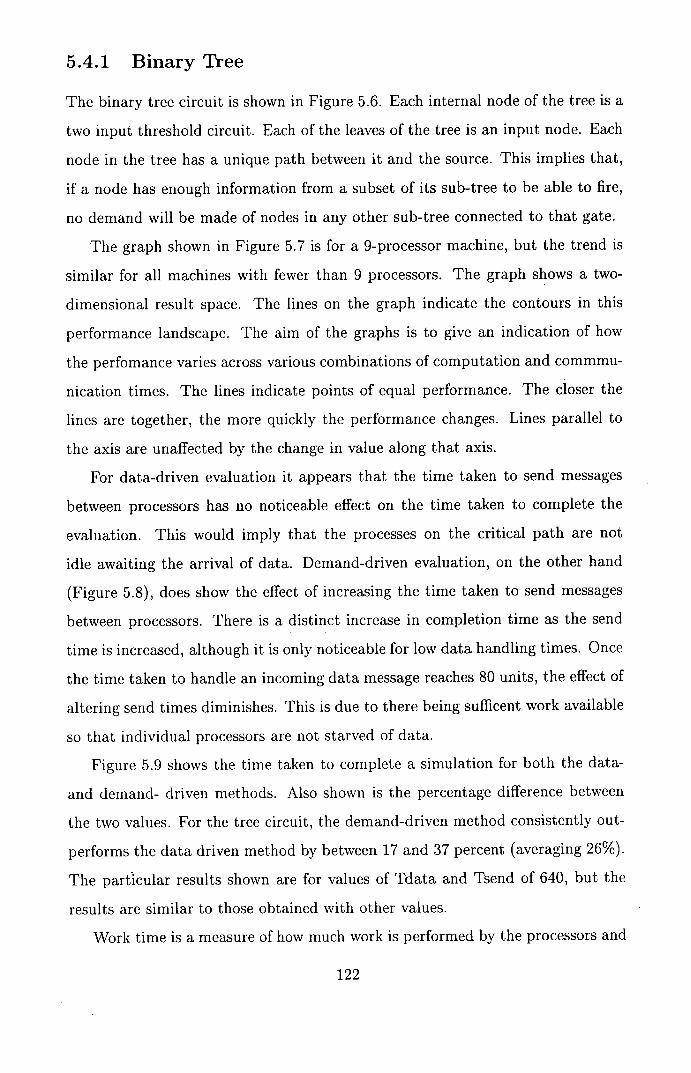
5.4.1 Binary Tree
The binary tree circuit is shown in Figure 5.6. Each internal node of the tree is a
two input threshold circuit. Each of the leaves of the tree is an input node. Each
node in the tree has a unique path between it and the source. This implies that,
if a node has enough information from a subset of its sub-tree to be able to fire,
no demand will be made of nodes in any other sub-tree connected to that gate.
The graph shown in Figure 5.7 is for a 9-processor machine, but the trend is
similar for all machines with fewer than 9 processors. The graph shows a two-
dimensional result space. The lines on the graph indicate the contours in this
performance landscape. The aim of the graphs is to give an indication of how
the perfomance varies across various combinations of computation and commmu-
nication times. The lines indicate points of equal performance. The closer the
lines are together, the more quickly the performance changes. Lines parallel to
the axis are unaffected by the change in value along that axis.
For data-driven evaluation it appears that the time taken to send messages
between processors has no noticeable effect on the time taken to complete the
evaluation. This would imply that the processes on the critical path are not
idle awaiting the arrival of data. Demand-driven evaluation, on the other hand
(Figure 5.8), does show the effect of increasing the time taken to send messages
between processors. There is a distinct increase in completion time as the send
time is increased, although it is only noticeable for low data handling times. Once
the time taken to handle an incoming data message reaches 80 units, the effect of
altering send times diminishes. This is due to there being sufficent work available
so that individual processors are not starved of data.
Figure 5.9 shows the time taken to complete a simulation for both the data-
and demand- driven methods. Also shown is the percentage difference between
the two values. For the tree circuit, the demand-driven method consistently out-
performs the data driven method by between 17 and 37 percent (averaging 26%).
The partcu1ar results shown are for values of Tdata and Tsend of 640, but the
results are similar to those obtained with other values.
Work time is a measure of how much work is performed by the processors and
122
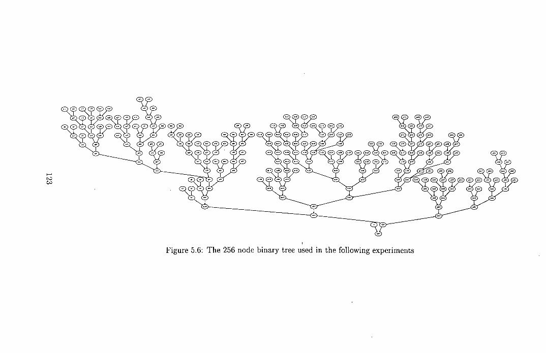
ND CAD
Figure 5.6: The 256 node binary tree used in the following experiments
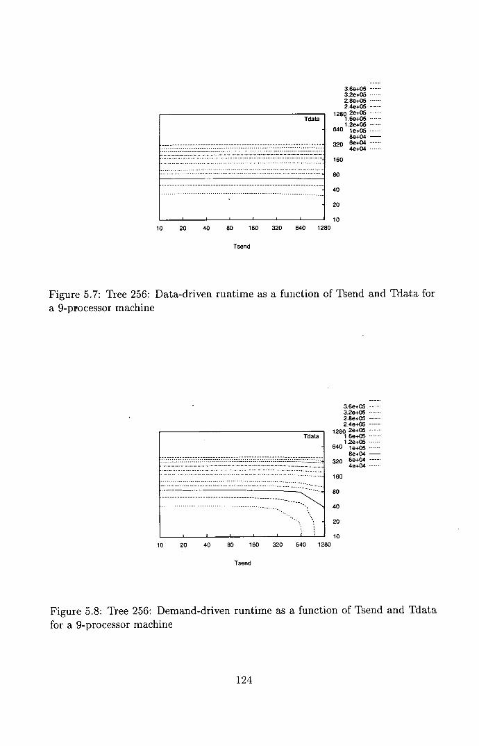
10 20 40 80 160 320
3.6e+05 3.2e+05 2.8e+05 ...... 2.4e+05
1280 2e+05 ----- Tdata 1.6e+05 ......
1.2e+05 ...... 640 1e+05 ......
8e+04 - o 6e+04
4e+04 ......
160
80
40
20
10 640 1280
Tsend
Figure 5.7: Tree 256: Data-driven runtime as a function of Tsend and Tdata for a 9-processor machine
3.6e+05 3.2e+05 ..... 2.8e+05 .......... 2.4e+05
10 20 40 80 160
Tsend
Tdata
640 le+05 ...... 8e+04 -
160
80
40
20
10
320 640 1280
Figure 5.8: Tree 256: Demand-driven runtime as a function of Tsend and Tdata for a 9-processor machine
124
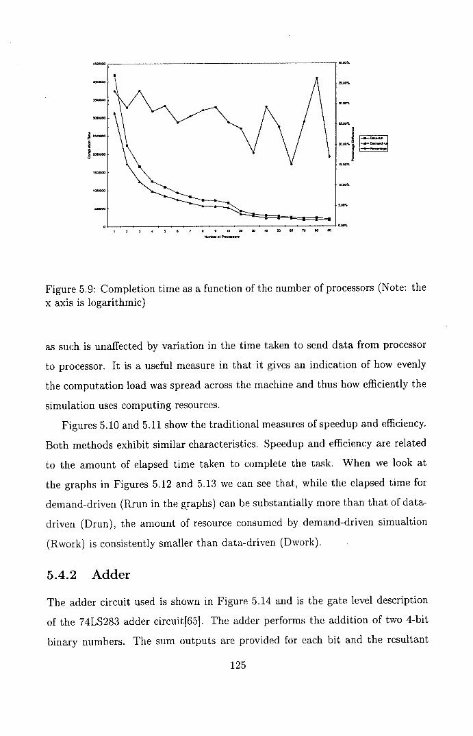
I
3%
3,.
3%
Figure 5.9: Completion time as a function of the number of processors (Note: the x axis is logarithmic)
as such is unaffected by variation in the time taken to send data from processor
to processor. It is a useful measure in that it gives an indication of how evenly
the computation load was spread across the machine and thus how efficiently the
simulation uses computing resources.
Figures 5.10 and 5.11 show the traditional measures of speedup and efficiency.
Both methods exhibit similar characteristics. Speedup and efficiency are related
to the amount of elapsed time taken to complete the task. When we look at
the graphs in Figures 5.12 and 5.13 we can see that, while the elapsed time for
demand-driven (Rrun in the graphs) can be substantially more than that of data-
driven (Drun), the amount of resource consumed by demand-driven simualtion
(Rwork) is consistently smaller than data-driven (Dwork).
5.4.2 Adder
The adder circuit used is shown in Figure 5.14 and is the gate level description
of the 74LS283 adder circuitt65l. The adder performs the addition of two 4-bit
binary numbers. The sum outputs are provided for each bit and the resultant
125
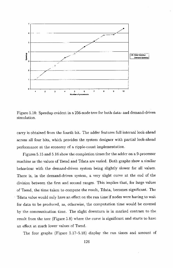
6
HData Speedup
Demand Speedup
2
0 1 2 3 4 5 6 7 6 9 10
Number of processors
Figure 5.10: Speedup evident in a 256-node tree for both data- and demand-driven simulation.
carry is obtained from the fourth bit. The adder features full internal look-ahead
across all four bits, which provides the system designer with partial look-ahead
performance at the economy of a ripple-count implementation.
Figures 5.15 and 5.16 show the completion times for the adder on a 9-processor
machine as the values of Tsend and Tdata are varied. Both graphs show a similar
behaviour with the demand-driven system being slightly slower for all values.
There is, in the demand-driven system, a very slight curve at the end of the
division between the first and second ranges. This implies that, for large values
of Tsend, the time taken to compute the result, Tdata, becomes significant. The
Tdata value would only have an effect on the run time if nodes were having to wait
for data to be produced, as, otherwise, the computation time would be covered
by the communication time. The slight downturn is in marked contrast to the
result from the tree (Figure 5.8) where the curve is significant and starts to have
an effect at much lower values of Tsend.
The four graphs (Figure 5.17-5.18) display the run times and amount of
126
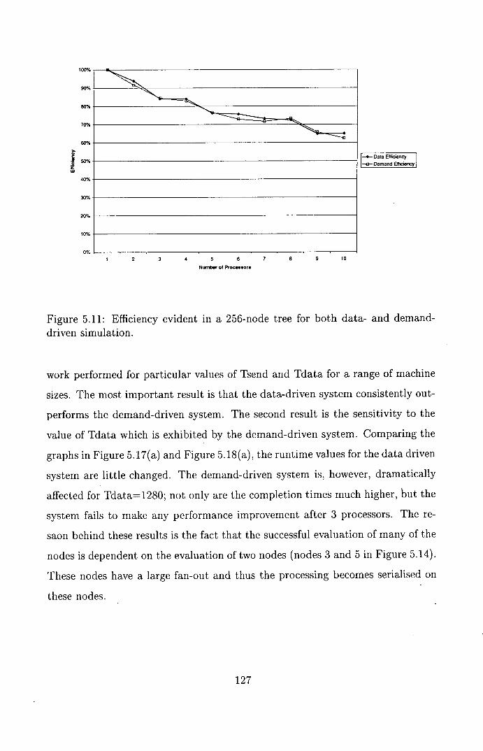
180%
90%
80%
70%
60%
C
50%
UI
40%
30%
20%
10%
0%
1-.--Data Efficiency
-e--Demand Efficiency
1 2 3 4 5 6 7 8 9 10
Number of Processors
Figure 5.11: Efficiency evident in a 256-node tree for both data- and demand-driven simulation.
work performed for particular values of Tsend and Tdata for a range of machine
sizes. The most important result is that the data-driven system consistently out-
performs the demand-driven system. The second result is the sensitivity to the
value of Tdata which is exhibited by the demand-driven system. Comparing the
graphs in Figure 5.17(a) and Figure 5.18(a), the runtime values for the data driven
system are little changed. The demand-driven system is, however, dramatically
affected for Tdata=1280; not only are the completion times much higher, but the
system fails to make any performance improvement after 3 processors. The re-
saon behind these results is the fact that the successful evaluation of many of the
nodes is dependent on the evaluation of two nodes (nodes 3 and 5 in Figure 5.14).
These nodes have a large fan-out and thus the processing becomes serialised on
these nodes.
127
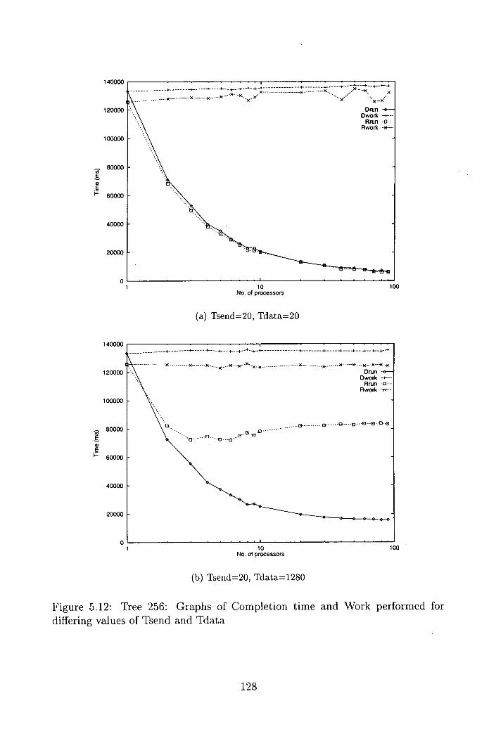
140000
120000
100000
80000 CO
E OC
E ' 60000
40000
20000
0 1
140000
120000
100000
80000 C,
E a, E
60000
40000
20000
0
•'x'.. x
Drun Dwork -----
Rrun .0-.-
Rwork •*--
10 100 No. of processors
(a) Tsend=20, Tdata=20
Drun -o--j Owork
Rrun 0•
Rwork )( ....
&........ 0 ...... .0 .....
.. B . Q
NO. OT processors
(b) Tsend=20, Tdata=1280
Figure 5.12: Tree 256: Graphs of Completion time and Work performed for differing values of Tsend and Tdata
128
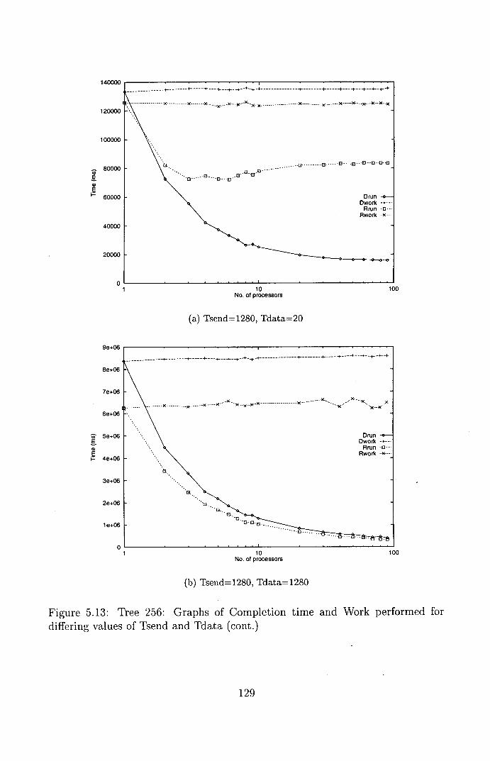
140000
120000
100000
- 80000 C.,
E 5, E
60000
40000
20000
0
+- - ------ -C--------
0 ...... 0 .0 .....
.0 ....... El ...E3...0
10 No. of processors
(a) Tsend= 1280, Tdata=20
Drun -.—H Dwork
Rrun 0-
Rwori ••x....
100
9e+06
8e+06
7e+06
6e+06
13 58+06 E 5, E
i 4e+06
3e+06
2e+06
le+06
C,
13.
Drun -e---Owork -4-- -
Rrun -0-
Rwork --C' ....
...
10 100 No. of processors
(b) Tsend=1280, Tdata=1280
Figure 5.13: Tree 256: Graphs of Completion time and Work performed for differing values of Tsend and Tdata (cont.)
129
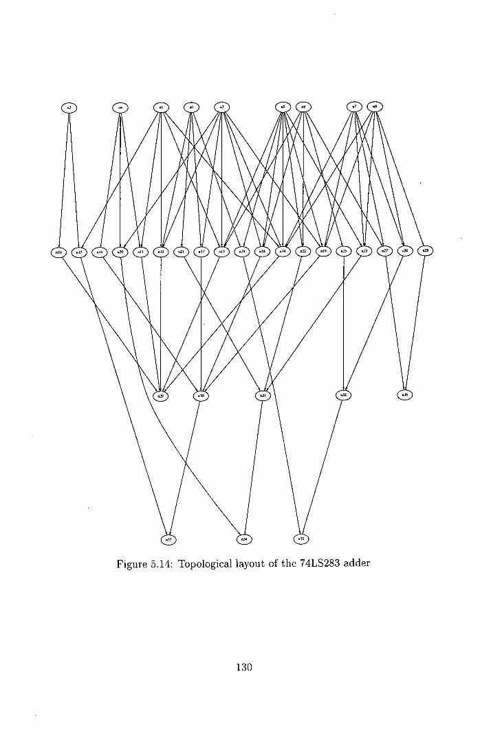
Figure 5.14: Topological layout of the 74LS283 adder
130
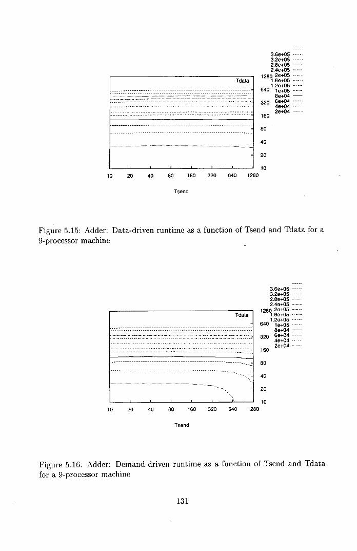
3.6e+05 3.2e+05 - 2.8e+05 ..........
2.4e+05
10 20 40 80 160 320
Tsend
1200 1.6e+05 1.2e-i-05
640 1e-+-05 8e+04
320 6e+04 4e+04 2e+04
160
80
40
20
10 640 1280
Tdata
Figure 5.15: Adder: Data-driven runtime as a function of Tsend and Tdata for a 9-processor machine -
3.6e+05 3.2e+05 ------ 2.8e-+-05 ...........
2.4e+05
10 20 40 80 160 320
Tsend
uou
1.2e-i-05 ------ 640 1e+05 ------
8e+04 320 6e+04
4e-s-04 ......
2e+04 ..........
160
80
40
20
10 640 1280
Tdata
Figure 5.16: Adder: Demand-driven runtime as a function of Tsend and Tdata for a 9-processor machine
131
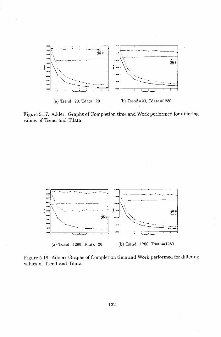
(a) Tsend=1280, Tdata=20
(a) Tsend=20, Tdata=20 (b) Tsend=20, Tdata=1280
Figure 5.17: Adder: Graphs of Completion time and Work performed for differing values of Tsend and Tdata
Figure 5.18: Adder: Graphs of Completion time and Work performed for differing values of Tsend and Tdata
132
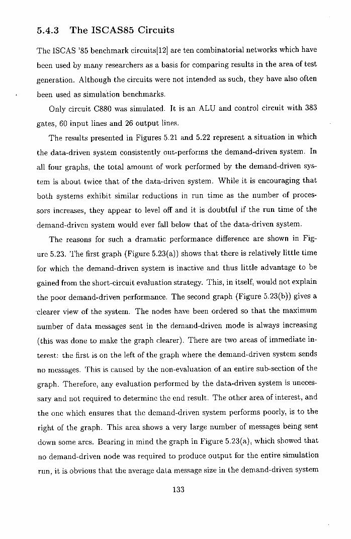
5.4.3 The ISCAS85 Circuits
The ISCAS '85 benchmark circuits[12] are ten combinatorial networks which have
been used by many researchers as a basis for comparing results in the area of test
generation. Although the circuits were not intended as such, they have also often
been used as simulation benchmarks.
Only circuit C880 was simulated. It is an ALU and control circuit with 383
gates, 60 input lines and 26 output lines.
The results presented in Figures 5.21 and 5.22 represent a situation in which
the data-driven system consistently out-performs the demand-driven system. In
all four graphs, the total amount of work performed by the demand-driven sys-
tem is about twice that of the data-driven system. While it is encouraging that
both systems exhibit similar reductions in run time as the number of proces-
sors increases, they appear to level off and it is doubtful if the run time of the
demand-driven system would ever fall below that of the data-driven system.
The reasons for such a dramatic performance difference are shown in Fig-
ure 5.23. The first graph (Figure 5.23(a)) shows that there is relatively little time
for which the demand-driven system is inactive and thus little advantage to be
gained from the short-circuit evaluation strategy. This, in itself, would not explain
the poor demand-driven performance. The second graph (Figure 5.23(b)) gives a
clearer view of the system. The nodes have been ordered so that the maximum
number of data messages sent in the demand-driven mode is always increasing
(this was done to make the graph clearer). There are two areas of immediate in-
terest: the first is on the left of the graph where the demand-driven system sends
no messages. This is caused by the non-evaluation of an entire sub-section of the
graph. Therefore, any evaluation performed by the data-driven system is uneces-
sary and not required to determine the end result. The other area of interest, and
the one which ensures that the demand-driven system performs poorly, is to the
right of the graph. This area shows a very large number of messages being sent
down some arcs. Bearing in mind the graph in Figure 5.23(a), which showed that
no demand-driven node was required to produce output for the entire simulation
run, it is obvious that the average data message size in the demand-driven system
133
was much smaller than that in the data-driven case. This may well be because
of greater interval fragmentation caused by the interaction of both demand and
data messages on the state space of the node over time.
7.5e+06 4.5e+06 ...... 1.5e+06 ..........
8e+05 1280 4e-f05
640
320
160
80
40
20
10
10 20 40 80 160 320 640 1280
Tsend
Figure 5.19: C880: Data-driven runtime as a function of Tsend and Tdata for a 9-processor machine
5.4.4 Linear Shift Register
This benchmark was proposed by Greer[371 as a quick and simple circuit which
could be constructed easily and scaled to stress the simulating system. The
benchmark is constructed by connecting a number of "base units" in series and
then putting a feedback loop which, when gated with the input, feeds the first
unit. The simplest base unit is a D-type flip-flop.
Shown in Figure 5.24 are N series-connected edge triggered D-type flip-flop
units. As shown, these flip-flop units are connected as a shift register with a
feedback from unit M. When the value of M is correctly chosen relative to N,
and when the output of the last unit is connected to the input of the first, a
linear feedback shift register (LFSR) is formed. By repeatedly clocking such a
134
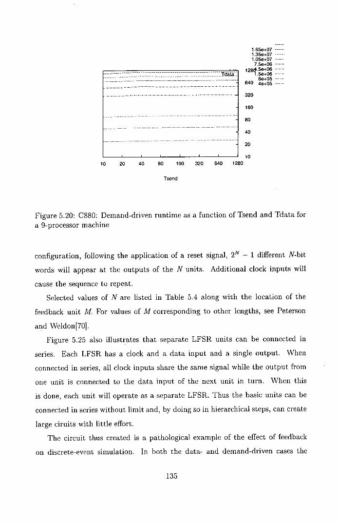
1.65e+07 1.35e+07 1.05e+07 7.5e+06
128.506 1.5e+06
8e-i-05 640 4e+05
320
160
80
- 1 40
•1 20
10
10 20 40 80 160 320 640 1280
Tsend
Figure 5.20: C880: Demand-driven runtime as a function of Tsend and Tdata for a 9-processor machine
configuration, following the application of a reset signal, 2N - 1 different N-bit
words will appear at the outputs of the N units. Additional clock inputs will
cause the sequence to repeat.
Selected values of N are listed in Table 5.4 along with the location of the
feedback unit M. For values of M corresponding to other lengths, see Peterson
and Weldon[70].
Figure 5.25 also illustrates that separate LFSR units can be connected in
series. Each LFSR has a clock and a data input and a single output. When
connected in series, all clock inputs share the same signal while the output from
one unit is connected to the data input of the next unit in turn. When this
is done, each unit will operate as a separate LFSR. Thus the basic units can be
connected in series without limit and, by doing so in hierarchical steps, can create
large ciruits with little effort.
The circuit thus created is a pathological example of the effect of feedback
on discrete-event simulation. In both the data- and demand-driven cases the
135
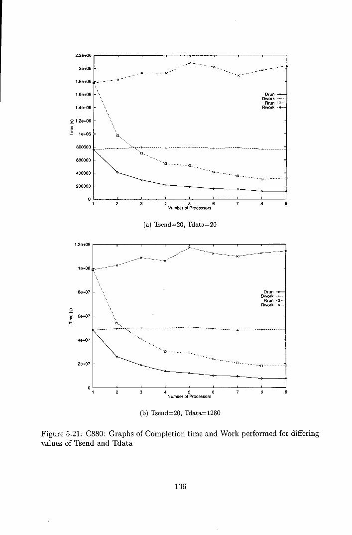
2.2e+06
2e+06
1.8e+06
1.6e+06
1.4e+06
i l.2e+06
i le+06
800000
600000
400000
200000
A
• ••.-• Drun e- Dwork -i---.
Rrun -O-
Rwork )(
= 1 2 3 4 5 6
7 8 9
Number of Processors
(a) Tsend=20, Tdata=20
1.2e+08
16+08
8e+07
Co
6e+07
I-
4ei-07
2e+07
A
x.... ................... . x....- ...
...
Drun -8--
Dwork -4---
Rrun -0-.
Rwork )(
0
1 2 3 4 5 6 7 8 9 Number of Processors
(b) Tsend=20, Tdata= 1280
Figure 5.21: C880: Graphs of Completion time and Work performed for differing values of Tsend and Tdata
136
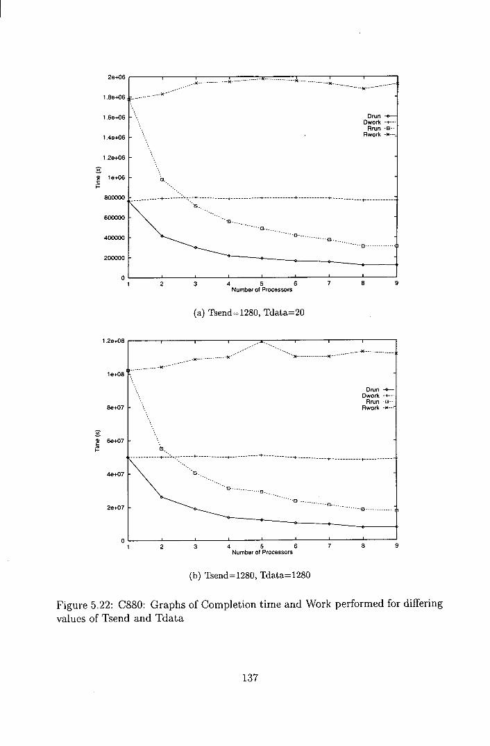
2e+06
1.8e+06
1.6e+06 • Drun Dwork -+--.
Awn D•
1.4e+06 Rwork ••M'••-'
1.2e+06
U,
18+06 C.
I-
800000
600000
13
400000
200000
1 2 3 4 5 6 7 8 9 Number of Processors
(a) Tsend= 1280, Tdata=20
1.2e+08
le+08
8e+07
(0
6e+07
I.-
4e+07
2e+07
I I I I
......... .. ........ ................
U, ... x. ............... U,........
U,
Drun ---Dworfc -i--
Rrun •• Rwork
1 2 3 4 5 6 7 8 9 Number of Processors
(b) Tsend=1280, Tdata=1280
Figure 5.22: C880: Graphs of Completion time and Work performed for differing values of Tsend and Tdata
137
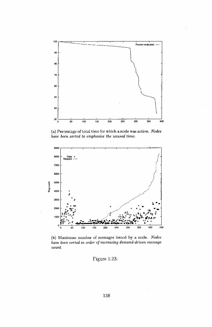
100
90
80
70
60
50
40
Percent evaluated -
301 I I I I I
0 50 100 150 200 250 300 350 400
Percentage of total time for which a node was active. Nodes have been sorted to emphasize the unused time.
9000 I
8000 Data 0
Request -----
7000
6000
5000 I
/ 01
4000 0
8
3000 08
• -------, . 0 .
o 0
2000 0, 10 / 0 0
000
0 •° :
1000 0 0
0ou00 o 0
0 0
0 8 0 1 0
0 50 100 150 200 250 300 350 400 450
Maximum number of messages issued by a node. Nodes have been sorted in order of increasing demand-driven message count.
Figure 5.23:
138
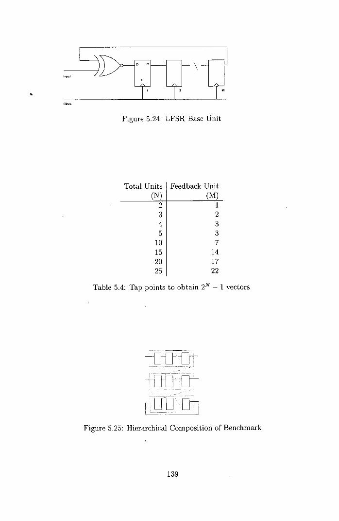
06
C'ock
Figure 5.24: LFSR Base Unit
Total Units I Feedback Unit (N) (M)
2 1 3 2 4 3 5 3
10 7 15 14 20 17 25 22
Table 5.4: Tap points to obtain 2 1" - 1 vectors
Figure 5.25: Hierarchical Composition of Benchmark
139
performance is poor. The effect that this has is to divide, and re-divide, the time
intervals until the system reaches a state of unit time intervals. In the case of
the demand-driven system, as well as the interval fragmentation to be considered,
there is also the fact that the base logic elements maintain internal state. Their
current state is some function of their previous state and the input applied. This
means that, without some reset signal being applied, to determine their current
state, we need to evaluate all previous states back to the start of the simulation
time. Once such demands for data have been sent, we are in a data-driven mode
without any of the short-circuiting, or sub-circuit evaluation, that demand-driven
system rely upon for performance.
5.4.5 Causes of Fragmentation
In ELSA, whenever a tuple arrives an output is generated for the fully defined
interval. The end time of the output tuple is the minimum of the end times
of the input tuples. The net result is that, potentially, the output stream will
be more fragmented than the input streams. The amount of fragmentation will
depend upon how misaligned the input streams are and the average size of the
input intervals.
If the intervals are misaligned by only a small amount then the output stream
will consist of tuples representing the misalignment and tuples representing the
larger, common, data areas. Should the average interval of one of the input
streams be small then the output stream will consists of intervals which are no
larger than those of the small interval input stream.
5.4.6 Example of fragmentation
Table 5.5 shows the number of intervals of a given size which occurred in the
demand-driven simulation of a 16-element LSR while Table 5.6 shows the number
which needed to occur to carry the data. The figures were obtained from an
analysis of the data messages sent during the course of the simulation. If two
contiguous tuples carried the same state value, then they were combined into a
single tuple. This process was repeated until every tuple carried a different state
140
Size of interval Count 1 699606 2 45859 3 30809
4 11862
5 2971
6 1786
7 431
8 93
9 146
10 760
Size of interval 1 2 3 4 5 6 7 8 9
10
Count 7433 5911 2856
514 542 795
16 8 7
455
Table 5.5: Actual Interval Counts Table 5.6: Minimum Interval Counts
to the immediately preceding and succeeding tuple.
The disparity between the figures shows that significantly more messages are
actually sent than would be needed if there was no tuple fragmentation.
The weighted mean values for interval size are 13.65 time units and 86.59
time units respectively. The weighted mean is the mean of the product of interval
size and count. Given that the input waveform has an average interval of 100
time units and the average gate delay is 3 time units the actual results show a
significant degradation of the interval.
Further analysis revealed that the median interval size for the actual results
is 1. That is to say that half the messages in the system represent intervals of
one time unit. The minimum results have a median of 85. This emphasises the
larger interval of the minimum results.
5.5 Conclusions
The general conclusion from the results gathered is that it is possible for the
demand-driven system to out-perform the data-driven system. There is a per-
formance gain in that it is possible for the demand-driven system to finish the
task sooner than the data-driven system. There is also the gain in resource
utilisation in that less of the machine's processor time needs to be used in the
demand-driven system. While this result is less important in the area of dedi-
cated single-user parallel machines, in the increasingly common scenario where a
parallel resource is shared (such as a network of workstations) a lower resource
141
requirement may permit more than one simulation run to be performed at the
same time (replication-parallelism).
What is, perhaps, more interesting is why the demand-driven system some-
times fails to out-perform the data-driven system. It would appear that the per-
formance of the demand-driven system is very dependent on the structure of the
system being evaluated. Even when the demand-driven system performs poorly,
many, if not all, nodes are not evaluated for all time. In some cases, the nodes
were only evaluated for 50% or less of the simulation time. Also, it is possble
to observe that some nodes in a demand-driven system seem to be issuing a far
greater number of messages than they do when evaluating under a data-driven
strategy.
Coupling the two observations, we can see that some nodes in a demand-
driven system are issuing a large number of tuples for very small intervals. As
each tuple must be handled, which causes further fragmentation of the tuple
stream, the resultant increase in run time is the inevitable result. An improved
ordering of nodes for evaluation may help to improve this situation (the current
method is only applicable to tree structures and assumes that the order in which
nodes are evaluated does not affect the evaluation time of any other node.) Also,
various tuple recombination strategies may help to quench the explosion in the
numbers of small tuples.
5.6 Chapter summary
In this chapter, a test-bed system was described which was used as a platform for
the simulation of both data- and demand-driven simulation systems. A number
of logic circuits were simulated on this test-bed and their performance character-
istics measured. As data-driven, conservative systems cannot support dynamic
topologies, the systems simulated had to be static. Their dynamic nature was
examined and we focussed on the effect on parallelism and performance as the
available computing resource increased.
The pathological example of a linear feedback shift-register was presented
which, as a result of the nested feedback loops, caused both the data- and demand-
142

driven system to perform badly as a result of the large number of small tuples
that both systems sent. The interval size for the data messages was fragmented
until both system were, in effect, working with unit time intervals. The demand-
driven system was required to request the state of all the elements for all time
which then left it operating in a data-driven mode.
143
Chapter 6
Summary and Conclusions
In this chapter we will summarise our work, discuss our conclusions and give some
directions for further work in the area of demand-driven systems.
6.1 Summary of thesis
In Chapter 1, we surveyed the state of the art in distributed simulation and
covered the characteristics of the two main systems (conservative - Chandy-Misra-
Bryant and optimistic - Time Warp). We noted that neither of these systems has
all of the attributes of the desired simulation system.
Chapter 2 looked at the background to the issues and we stepped back from
simulation and studied the more generic problems of the production and synchro-
nisation of data in a distributed system. We saw that, by making the receiver
responsible for requesting the data rather than have it wait passively, we could
obtain a dynamic topology for inter-element connections.
We also clarified the difference between request-driven and demand-driven
systems and looked at related work at the micro, compiler and language levels.
Related work in simulation, using either demand-driven or request-driven systems,
was also discussed.
Definitions of speedup and efficiency, that are widely used throughout the
distributed systems field as quality measures, were discussed and we proposed a
new measure, opportunity cost, to give an indication of how much of the systems
resources are withheld from other potential users.
The chapter closed by looking at binary decision diagrams. This method of
144
expressing a function can make explicit any non-strictness in that function and
as such, is well placed to be utilised in a demand-driven system.
The benefits that are inherent in a demand-driven system were outlined in
Chapter 3. It also addressed the more obvious shortcomings of the method and
looked at ways to mitigate their effect. Threshold functions were introduced as a
tool to address the question of the strictness of a function. The work of Dunne
and Leng311 was introduced as an approach to minimising the work required to
evaluate a function. This approach was then expanded to consider the evaluation
of the function on a parallel machine through the use of input and output modes.
Chapter 4 described three simulation systems: ELSA 151, a data-driven interval
based system, CMB[19], a data-driven event based system and our proposed
demand-driven interval based system. Analytical models for the upper bound
of the number of messages needed and the processing resource consumed were
derived and some suggestions on how to make the upper bound more accurate
were made.
The chapter continued with a discussion on the effect of the model's inabil-
ity to handle non-independent streams effectively. Random binary trees were
generated and, as they exhibit independent data streams, were used to predict
the expected performance of ELSA and demand-driven system. The results of
the models were presented in a number of graphs which show the effect of vary-
ing granularity, frequency of events and strictness on both the communications
bandwidth required and the processing resources consumed.
Experimental results were presented in Chapter 5. A test-bed system was
described which was used as a platform for the simulation of both data- and
demand-driven simulation systems. A number of logic circuits were simulated
on this test-bed and their performance characteristics measured. As data-driven,
conservative systems cannot support dynamic topologies, the systems simulated
had to be static. Their dynamic nature was examined and we focussed on the
effect on parallelism and performance as the available computing resource in-
creased.
The pathological example of a linear feedback shift-register was presented
145
which, as a result of the nested feedback loops, caused both the data- and demand-
driven systems to perform badly. The interval size for the data messages was
fragmented until both systems were, in effect, working with unit time intervals.
The demand-driven system was required to request the state of all the elements
for all time which then left it operating in a data-driven mode.
6.2 Further work
Throughout the investigation into demand-driven discrete event simulation, a
number of questions remained unanswered.
6.2.1 The function/cache dichotomy
The model of demand-driven evaluation which we have used throughout the thesis
is one where the node is foremost and the cache of previously computed results is
an adjunct to it. That is to say that the node receives and processes the request,
either by consulting the cache or by sparking a new computation. This "function
centric" view of the system, while simple to implement, is limiting. An alternative
approach would be to reverse the view, to treat the system as "smart memory", by
putting the cache first as the main recipient of requests and make it responsible
for sparking new computation.
The potential advantage of this approach is that, while the memory (cache)
would reside in fixed locations, the nodes responsible for calculating the function
could be spread throughout the system. This opens up the possibility of relatively
fine grain load balancing as each new functional evaluation could be started on
the "best" available resource.
6.2.2 Hierarchical evaluation
A simulation model is created from an abstraction of the features of the physical
system under investigation. The features chosen for the simulation model may
well be some way removed from the physical implementation of those features,
e.g. a wire in a digital circuit will have a number of physical attributes (potential,
current, capacitance etc.). These will, in some models, be simplified to a single
146
logical value of true or false. While it is common for the level of abstraction to
be uniform across the entire system, and it is less common to have different, but
fixed, levels of abstraction within one simulation, standard data-driven methods
do not permit the system to alter the level of abstraction dynamically in response
to internal conditions. This might be triggered by a condition arising which
cannot be modelled successfully at the level of abstraction chosen. A lower level
of abstraction would then need to be used. However, to simulate the entire system
at the lower level in case such a situation occurred may be impractical due to time
or processor constraints.
Demand-driven simulation may be able to address the issue of dynamically
altering the level of abstraction in response to local conditions. Should a condition
arise that needs to be resolved at a lower level, then the node could request that
information at the appropriate level. Further work would be needed to assess the
need for such an adaptive system as well as the overhead involved.
6.2.3 Managing load in a peer-to-peer network
Moving away from simulation, an interesting piece of further work would to in-
vestigate the extent to which the techniques of demand-driven evaluation can be
applied to the emerging peer-to-peer networks.
Assuming a network of web application providers, a user could submit some
task to the network. The local node in the network may well be able to perform
the work itself or it may choose to send a sub-task to another node.
6.3 Conclusion
Whether the benefits of demand-driven simulation can be exploited depends on
the specific situation to which it is applied.
The biggest performance gain in demand-driven simulation comes from non-
strict nodes. These nodes give rise to the possibility of not requiring to evaluate
large sections of the underlying system graph and thus reduce the amount of work
which needs to be performed. This reduction in required evaluation leads, quite
directly, through to reduced communication and processor loads. These reduced
147
loads can often more than compensate for the higher loads imposed by a demand-
driven system compared with a data driven system. There is, however, an open
question about how strict simulation functions actually are, in practice.
Demand-driven systems also perform well in situations where nodes have a
low active, output connectivity. Active connectivity relates to links which are
actually used rather than being logical connections. This reduces the chances
of two nodes requesting similar (but slightly different) time intervals and thus
causing increased fragmentation. The more nodes there are requiring the output
from another node, the greater the chance of fragmentation. The pathological case
of the low output connectivity would be the tree. It is not surprising, therefore,
that the tree structure using non-strict nodes shown in Section5.4.1 performed
well.
The most striking problem which arises in demand-driven simulation is the
potential for an explosion in the number of tuples used to transmit the data
between nodes. This problem is the mirror of one which affects the data driven
system. The demand-driven system has both to contend with its calendar being
fragmented both by request messages and by data messages. If more than one
node requests data over two specific (and overlapping) intervals then both requests
will be fractured resulting, in all probability, in an increase in the number of tuples
sent to each requester. This increase can easily swamp any gain achieved by using
non-strict nodes.
Determining whether two tuples can be recombined is a relatively trivial task
(as long as the states carried can be compared for equality). The only difficulty
is to ensure that no deadlock conditions are added to the system by the recom-
bination. The safest place to perform the combination would be in the cache as
it does not reply on any other data for its functioning and as such, the worst
overhead would be a delay. Tuples can be recombined at other locations as well
if suitable buffers are created.
A related issue which requires special handling to operate efficiently is feed-
back. As in data driven systems, feedback can cause an explosion in the amount
of work required to be performed. In the demand-driven case we have the situ-
ation that a node is dependent on its own earlier results to process the current
request. This can continue until the node reaches some base case, which may be
the initialisation state at the start of simulation time. The node would roll further
and further back in time issuing requests and then roll forward again acting as if
it was a data driven node. Each request would, in the simplest case, fragment the
interval further. The extreme case would have a node stepping forward in time
by the delay through the loop even if the data state did not change. This can be
handled more efficiently in both data and demand-driven systems.
While demand-driven systems can handle variable (but bounded) delays, it
becomes increasingly less efficient at doing so as the bounds on the interval in-
crease. In the extreme example of a node holding a state until some other node
sends a signal (quite common in handshaking protocols) then the node holding
the signal does not know when the other node is going to send its signal and
has, therefore, to hunt back in time until it finds one. Each request causes an
overhead as well as increasing the fragmentation. In general, such protocols will
hunt back to the start of simulation time and then advance in the normal data
driven manner.
While the potential for improved performance depends on the situation to
which demand-driven evaluation is applied, there are other gains to be made from
using a demand-driven system. The most notable one is partial activation. The
need for this feature may be sufficient to make any potential overhead worthwhile
carrying.
Partial activation allows the simulationist to place a probe in the system and
cause only those nodes whose results are needed to generate a result at the probe
to activate. This has the potential to render large parts of the system inactive
and thus save on processing power. A similar effect could be achieved in a data
driven system by a pre-processing step which could determine all those nodes
whose results might be needed. The demand-driven system obviates this step as
determining the necessary nodes is a function of the basic simulation step.
A side effect of partial evaluation is that the necessary input signals to sub-
circuits are automatically generated (assuming that suitable signals are available
149

to the primary inputs). This removes the need (which would exist within a data
driven system) of creating accurate sub-circuit input signals.
Demand-driven discrete event simulation, using time intervals, is able to pro-
vide a platform with dynamic communication between the nodes, local control
of processing, efficiently uses processor power, and is conservative. If the struc-
ture being simulated is free from deadlock, then the simulation will be also. The
client-server approach means that the evaluation is easy to distribute over avail-
able processors. The use of a calendar and time intervals means that the system
is able to automatically identify, and exploit, both structural and temporal par-
allelism in the underlynig system.
150
Bibliography
ADAMS, D. A model for parallel computations. In Parallel Processor Sys-
tems, Technologies, and Applications, L. Hobbs, Ed. Spartan, 1970, pp. 311-
333.
AGRAWAL, P. Concurrency and communication in hardware simulators.
IEEE Trans. on Computer-Aided Design CAD-5, 4 (Oct. 1986), 617-623.
131 AKERS, S. B. Binary decision diagrams. IEEE Transactions on Computers
C-27, 6 (Aug. 1978), 509-516.
11 ARVIND, AND IANNUCCI, R. Two fundamental issues in multiprocessing.
Computation Structures Group Memo 226-5, MIT Computer Science Lab,
July 1986.
151 ARVIND, D., AND SMART, C. A unified framework for parallel event-driven
logic simulation. In Proceedings of the 1991 Summer Computer Simulation
Conference (July 1991), SCS, pp. 92-97.
[6] ARVIND, D., AND SMART, C. Hierarchical parallel discrete event simula-
tion in composite elsa. In Proceedings of the 1992 ACM/IEEE Conference
on Parallel and Distributed Simulation (Newport Beach, CA, Jan. 1992),
ACM/IEEE.
171 AVRIL, H., AND TROPPER, C. Scalable clustered time warp and logic
simulation. VLSI Design 9, 3 (1999), 291-313.
[8] BAUER, H., SPORRER, C., AND KRODEL, T. H. On distributed logic
simulation using time warp. In VLSI 91 (1991), pp. 4a.1.1-4a.1.10.
151
BELLENOT, S. Global virtual time algorithms. In Proceedings of the SCS
Multiconference on Distributed Simulation (January 1990), vol. 22, pp. 122-
127.
BIRD, R. Introduction to Functional Programming using Haskell. Prentice
Hall Press, 1998.
BRADLEY, E., AND HALSTEAD, R. H. Simulating logic circuits: A multi-
processor application. International Journal of Parallel Programming 16, 4
(1987),305-338.
BRGLEZ, F., POWNALL, P., AND Hum, R. Accelerated ATPG and fault
grading via testability analysis. In Proceedings of the International Sympo-
sium on Circuits and Systems (1985).
BRYANT, R. Simulation of packet communication architecture computer sys-
tems. Tech. Rep. MIT-LCS-TR-188, Massachusetts Institute of Technology,
1977.
BRYANT, R. Graph-based algorithms for boolean function manipulation.
IEEE Transactions on Computers C-35, 8 (1986), 677-691.
BRYANT, R. Symbolic boolean manipulation with ordered binary-decision
diagrams. Computing Surveys 2, 3 (1992), 293-318.
BUTLER, J., AND WALLENTINE, V. Message bundling in Time-Warp. Tech-
nical Report TR-CS-90-8, Department of Computing and Information Sci-
ences, Kanas State University, Sept. 1990.
CAI, W., AND TURNER, S. An algorithm for distributed discrete-event
simulation - the 'carrier null' approach. In Proceedings of the SCS Multicon-
ference on Distributed Simulation (January 1990), vol. 22, pp. 3-8.
CA0, J., AND WANG, K. Efficient synchronous checkpointing in distributed
systems. Tech. Rep. 91/6, James Cook University of North Queensland, Dec.
1991.
152
1191 CHANDY, K., AND MISRA, J. Asynchronous distributed simulation via a
sequence of parallel computations. Commun. ACM 24, 11 (Apr. 1981), 198-
206.
CHANDY, K., MISRA, J., AND HAAS, L. Distributed deadlock detection.
ACM Transactions on Computer Systems 1, 2 (May 1983), 144-156.
CHARLTON, C., JACKSON, D., AND LENG, P. Lazy simulation of digital
logic. Computer-Aided Design 23, 7 (Sept. 1991), 506-513.
CHARLTON, C., JACKSON, D., LENG, P., AND RUSSELL, P. Modelling
circuit delays in a demand driven simulator. Computers and Electrical En-
gineering 20, 4 (1994), 309-318.
C0TA, B., AND SARGENT, R. An algorithm for parallel discrete event
simulation using common memory. Simulation Digest 20, 1 (Mar. 1989),
23-31.
DAvis, A., AND KELLER, R. Data-flow program graphs. IEEE Computer
15, 2 (Feb. 1982), 26-41.
DENNIS, J. The evolution of 'static' data-flow architecture. In Advanced
Topics in Data-Flow Computing, J.-L. Gaudiot and L. Bic, Eds. Prentice-
Hall, Englewood Cliffs, NJ, 1991, pp. 35-91.
DENNIS, J., AND MISUNAS, D. A computer architecture for highly parallel
signal processing. In Proceedings of the 1974 National Computer Conference
(1974), AFIPS Press, pp. 402-409.
DEUTSCH, J., AND NEWTON, A. A multiprocessor implementation of
relaxation-based electrical circuit simulation. Proceedings of the 21st De-
sign Automation Conference (1984), 350-357.
DICKENS, P., AND REYNOLDS, P. SRADS with local rollback. In Proceed-
ings of the SCS Multiconference on Distributed Simulation (January 1990),
vol. 22, pp. 161-164.
153

[29) D'SouzA, L., FAN, X., AND WILSEY, P. pGVT: An algorithm for accu-
rate GVT estimation. In Proc. of 8th Workshop on Parallel and Distributed
Simulation (July 1994), PP. 102-109.
DUNNE, P., GITTINGS, C., AND LENG, P. Sequential and parallel strate-
gies for the demand-driven simulation of logic circuits. Microprocessing and
Microprogramming 38 (1993), 519-525.
DUNNE, P. E., AND LENG, P. H. An algorithm for optimising singal selec-
tion in demand-driven digital circuit simulation. Transactions of The Society
for Computer Simulation 8, 4 (Dec. 1991), 269-293.
EAGER, D. L., ZAHORJAN, J., AND LAZOWSKA, E. D. Speedup versus
efficiency in parallel systems. IEEE Transactions on Computers 38, 3 (Mar.
1989),408-423.
FUJIM0TO, R. Time warp on a shared memory multiprocessor. Transactions
of the Society for Computer Simulation 6, 3 (July 1989), 211-239.
FujiMoTo, R. Parallel discrete event simulation. Commun. ACM 33, 10
(Oct. 1990), 31-53.
1351 FujiMoTo, R. M., T5AI, J.-J., AND GOPALAKRISHNAN, G. The roll-back
chip: hardware support for distributed simulation using time warp. In Proc.
of the SCS Multiconference on Distributed Simulation (Feb. 1988), B. Unger
and D. Jefferson, Eds., SCS, pp. 81-86.
[36) GAFNI, A. Roll-back mechanisms for optimistic distributed simulation. Dis-
tributed Simulation 19, 3 (88), 61-67.
GREER, D. L. The quick simulator benchmark. VLSI Systems Design 8, 12
(Nov. 1987), 40-57.
GROSELJ, B., AND TROPPER, C. The time-of-next-event algorithm. In
Proc. of the SCS Multiconference on Distributed Simulation (Feb. 1988),
B. Unger and D. Jefferson, Eds., vol. 19, SCS, pp. 25-29.
154
1391 HALSTEAD, R. New ideas in parallel lisp: Language design, implementation,
and programming tools. In Parallel Lisp: Languages and Systems, T. Ito and
R. H. Halstead, Eds. Springer, 1990, pp. 2-57.
1401 HALSTEAD, R. H. MultiLisp: a language for concurrent symbolic computa-
tion. ACM Trans. Program. Lang. Syst. (Oct. 1985), 501-538.
1411 HILLIs, W. D. The Connection Machine. The MIT Press, 1989.
[421 HOEGER, H., AND JONES, D. Integrating concurrent and conservative dis-
tributed discrete-event simulators. Simulation 67, 5 (1996), 303-314.
1431 HUGHES, R. Lazy memo functions. Lecture Notes in Computer Science 201
(Sept. 1985), 129-148.
[441 INGALLS, R., MORRICE, D., AND WHINSTON, A. Interval time clock im-
plementation for qualitative event graphs. In Proccedings of the 1994 Winter
Simulation Conference (1994), pp. 574-480.
[451 JEFFERSON, D. Virtual time. ACM Trans. Program. Lang. Syst. 7, 3 (July
1985),404-425.
146] JEFFERSON, D., HONTALAS, P., AND BECKMAN, B. Performance of the
Colliding Pucks simulation on the time warp operating systems. In Dis-
tributed Simulation (1989), Society for Computer Simulation, pp. 3-7.
1471 JEFFERSON, D, AND REIHER, P. Supercritical speedup. In The 24th
Annual Simulation Symposium (Apr. 1991), pp. 159-168.
1481 JEFFERSON, D., AND S0wIzRAL, H. Fast concurrent simulation using the
time warp mechanism. In Distributed Simulation 1985 (1985), P. Reynolds,
Ed., SCS, pp. 63-69.
191 JENNINGS, G., ISAKSSON, J., AND LINDGREN, P. Ordered ternary decision
diagrams and the multivalued compiled simulation of unmapped logic. In The
27th Annual Simulation Symposium (Apr. 1994), pp. 99-105.
155
[50] KORPELA, E., WERTHIMER, D., ANDERSON, D., COBB, J., AND LEBOF-
SKY, M. SETI©home: Massively distributed computing for SETI. IEEE
Computing in Science and Engineering 8, 1 (Jan/Feb 2001), 78-83.
151] LEUNG, E., CLEARY, J., LowMow, G., BEAZNER, D., AND UNGER, B.
The effects of feedback on the performance of conservative algorithms. In
Distributed Simulation (1989), Society for Computer Simulation, pp. 44-49.
[52] LIN, Y.-B., AND LAZOWSKA, E. D. The optimal checkpoint interval in
time warp parallel simulation. Tech. Rep. 89-09-04, Department of Computer
Science and Engineering, University of Washington, Seattle, WA, Sept. 1989.
[531 LIN, Y.-B., AND LAZOWSKA, E. D. Determining the global virtual time in
a distributed simulation. In International Conference on Parallel Processing
(1990), pp. 111-201-111-209.
UN, Y.-B., AND PREISS, B. Optimal memory management for time warp
parallel simulation. ACM Transactions on Modeling and Computer Simula-
tion 1, 4 (Oct. 1991), 283-307.
LIN, Y.-B., PREISS, B., LOUCKS, W., AND LAZOWSKA, E. D. Selecting
the checkpoint interval in time warp simulation. In Proc. of the 7th Workshop
on Parallel and Distributed Simulation (May 1993), pp. 3-10.
MADISETTI, V., WALRAND, J., AND MESSERSCHMITT, D. WOLF: a roll-
back algorithm for optimistic distributed simulation systems. In Proceedings
of the Winter Simulation Conference (San Diego, California, 1988), pp. 296-
305.
MCAFFER, J. A unified distributed simulation system. In Proccedings of
the 1990 Winter Simulation Conference (Dec. 1990), SCS, pp. 415-422.
MICHIE, D. 'Memo' functions and machine learning. Nature, 218 (April
1968),19-22.
1591 MINSKY, M. U., AND PAPERT, S. A. Perceptrons. MIT Press, 1988.
156
MISRA, J. Distributed discrete-event simulation. ACM Computing Surveys
18, 1 (March 1986), 39-65.
MOHR, E., KRANZ, D., AND HALSTEAD, R. Lazy task creation: A tech-
nique for increasing the granularity of parallel programs. IEEE Transactions
on Parallel and Distributed Systems 2, 3 (July 1991), 246-280.
MONSON-HAEFEL, R., AND CHAPPELL, D. Java Message Service. O'Reilly,
Dec. 2000.
MULLER, H., HARTEL, P., AND HERTZBERGER, L. Evaluation of abstract
simulation models. Collected Papers from the Second BCS PPSG Workshop
on Abstract Machine Models for Highly-Parallel Computers, Apr. 1993. Uni-
versity of Leeds.
MUROGA, S. Threshold Logic and its Applications. John Wiley and Sons,
Inc., 1971.
NATIONAL SEMICONDUCTOR. Logic Databook, 1981.
NIC0L, D. Parallel discrete-event simulation of FCFS stochastic queuing
networks. In Proceedings of the A CM/SIGPLAN Symposium on Principles
and Practice of Parallel Programming (1988), pp. 124-137.
NIKHIL, R., AND ARVIND. Can dataflow subsume von Neumann computing?
In Proceedings of the 16th International Symposium on Computer Architec-
ture (Jerusalem, Israel, May 1989), pp. 262-272.
NIKHIL, R., PAPADOPOULOS, G., AND ARVIND. *T : a multithreaded mas-
sively parallel architecture. In Proceedings of the 19th International Sympo-
sium on Computer Architecture (Brisbane, Australia, May 1992), pp. 156-
167.
PALANISWAMY, A. C., AND WILSEY, P. A. An analytical comparison
of periodic checkpointing and incremental state-saving. In Proc. of the 7th
Workshop on Parallel and Distributed Simulation (May 1993), pp. 127-134.
4
157
[70] PETERSON, W., AND WELDON, J. E. Error-Correcting Codes. The MIT
Press, 1972.
1711 PRAKASH, A., AND SUBRAMANIAN, R. Filter: An algorithm for reducing
cascaded rollbacks in optimistic distributed simulation. In The 24th Annual
Simulation Symposium (Apr. 1991), pp. 123-132.
PREISS, B., LOUCKS, W., MACINTYRE, I., AND FIELD, J. Null message
cancellation in conservative distributed simulation. Advances in Parallel and
Distributed Simulation 23 (Jan. 1991), 33-38.
PREISS, B., MACINTYRE, I., AND LOUCKS, W. On the trade-off between
time and space in optimistic parallel discrete-event simulation. In Proc. of the
6th Workshop on Parallel and Distributed Simulation (Jan. 1992), pp. 33-42.
RAJAEI, H., AYANI, R., AND THORELLI, L. The local time warp approach
to parallel simulation. In Proc. of 7th Workshop on Parallel and Distributed
Simulation (May 1993), pp. 119-126.
REIHER, P., FUJIMOTO, R., BELLENOT, S., AND JEFFERSON, D. Cancel-
lation strategies in optimistic execution systems. In Proceedings of the SCS
Multiconference on Distributed Simulation (January 1990), vol. 22, pp. 112-
121.
REYNOLDS, P. A spectrum of options for parallel simulation. In Proccedings
of the 1988 Winter Simulation Conference (Dec. 1988), SCS, pp. 325-332.
RODRIGUEZ, J. A graph model for parallel computation. Tech. Rep. ESLR-
398, MAC-TR-64, MIT Computer Science Lab, Sept. 1969.
SAMADI, B. Distributed Simulation Algorithms and Performance Analysis.
PhD thesis, University of California, Los Angeles, 1985.
179] SASSA, M., AND NAKATA, I. Time-optimal short-circuit evaluation of
boolean expressions. Information Processing Letters 29 (Sept. 1988), 43-
51.
158
SMITH, S. P. Progress in Computer-Aided VLSI Design, vol. 1. Ablex
Publishing Corporation, 1989, ch. Demand-Driven Simulation, pp. 191-233.
SMITH, S. P., MERCER, M. R., AND BROCK, B. Demand driven sim-
ulation: BACKSIM. In 24th ACM/IEEE Design Automation Conference
(1987), ACM/IEEE, pp. 181-187.
SOULE, L. Parallel-logic simulation: An evaluation of centralized and
distributed-time algorithms. Tech. Rep. TR-92-527, Coumputer Systems
Laboratory, Stanford University, 1992.
SOULE, L., AND GUPTA, A. Parallel distributed-time logic simulation. IEEE
Design & Test of Computers (Dec. 1989), 32-48.
STEINMAN, J. SPEEDES: A unified approach to parallel simulation. In Proc.
of the 6th Workshop on Parallel and Distributed Simulation (Jan. 1992),
pp. 75-83.
STEINMANN, J. Breathing time warp. In Proc. of the 7th Workshop on
Parallel and Distributed Simulation (May 1993), pp. 109-118.
STERLING, T., BECKER, D. J., SAVARESE, D., DORBAND, J. E.,
RANAWAKE, U. A., AND PACKER, C. V. BEOWULF: A parallel work-
station for scientific computing. In Proceedings of the 1995 International
Conference on Parallel Processing (ICCP) (Aug. 1995), vol. 1, pp. 22-30.
SUBRAMANIAN, K., AND ZARGHAM, M. Distributed and parallel demand
driven logic simulation. In 27th ACM/IEEE Design Automation Conference
(1990), pp. 485-490.
TEO, Y., AND TAY, S. Modelling and distributed simulation on a network
of workstations. International Journal of Modelling and Simulation 17, 3
(1997),208-216.
VEGDAHL, S. A survey of proposed architectures for the execution of func-
tional languages. IEEE Transactions on Computers C-23, 12 (Dec. 1984),
1050-1071.
159
1901 WAGNER, D., AND LAZOWSKA, E. Techniques for efficient shared-memory
parallel simulation. Tech. Rep. .TR-88-04-05, Department of Computer Sci-
ence, University of Washington, Seattle, Washington, Aug. 1988.
WAGNER, D., AND LAZOWSKA, E. Parallel simulation of queueing networks:
Limitations and potentials. In Proceedings of the ACM SIGMETRICS and
Performance, Vol 17, No. 1 (May 1989), pp. 146-155.
WAGNER, D. B., AND CALDER, B. Portable, efficient futures. Technical
Report CU-CS-609-92, University of Colorado at Boulder, Aug. 1992.
160


![Concurrent atomistic-continuum simulations of uniaxial ...€¦ · atomic trajectory inside the materials in experiments, numerical simulations via atomistic methods [11,12] and discrete](https://static.documents.pub/doc/80x56/5fb2485e21a30672d07b36b4/concurrent-atomistic-continuum-simulations-of-uniaxial-atomic-trajectory-inside.jpg)


![Discrete Control - Real-Time Systems, Lecture 14 · Discrete Control Real ... System: Chapter 12] 1. Discrete Event Systems 2. ... mechanism is time-driven. Continuous discrete-time](https://static.documents.pub/doc/80x56/5b1497697f8b9a3e7c8daf88/discrete-control-real-time-systems-lecture-14-discrete-control-real-system.jpg)


