Demand For Fuel Economy in the Indian Passenger Vehicle Market

Demand For Fuel Economy in the Indian PassengerVehicle Market∗

DRAFTDecember 29, 2009

Randy Chugh†Department of Economics

University of Maryland, College Park

Maureen Cropper‡Department of Economics

University of Maryland, College Parkand

Resources for the Future

Urvashi Narain§World Bank

Abstract

As the Indian automobile market continues its rapid expansion, concerns over the con-sequences of increased fuel consumption continue to grow. One potential response is fueleconomy regulation. One justification for fuel economy standards is the failure of consumersto choose optimally, due to myopia or market constraints. We evaluate the optimality ofconsumer responses to fuel economy in India by focusing on the choice between petrol anddiesel vehicles. Our first test asks whether it would be cheaper for the buyer of a petrol(diesel) vehicle to own and operate an otherwise identical diesel (petrol) vehicle. To do thiswe estimate hedonic price functions and fuel efficiency frontiers to predict what the chosenpetrol (diesel) vehicle, described in terms of weight, power, and other characteristics, wouldcost as a diesel (petrol) vehicle, and what its fuel economy would be. We use these resultsto estimate the break even period—the time it takes for the difference in purchase pricebetween otherwise identical diesel and petrol vehicles to equal the present discounted valueof fuel savings—and compare this to expected vehicle life. Because this assumes that eachpetrol vehicle is available in diesel form, we also compare the difference in purchase priceplus operating cost between the chosen petrol vehicle and the average diesel sold. This isa lower bound to the difference between what a petrol owner is willing to pay for a morepowerful, but less fuel efficient petrol car and the average diesel car.

∗We thank Rob Williams and Hendrik Wolff for helpful suggestions and John Allen Rogers for many usefuldiscussions and assistance in obtaining data. We also thank seminar participants at University of Maryland,College Park and at the 2009 Western Economic Association International conference in Vancouver, BritishColumbia. This paper was funded by the World Bank’s KCP Trust Fund. The findings and conclusions ofthis paper are those of the authors and do not necessarily represent the views of the World Bank and itsaffiliated organizations, the Executive Directors of the World Bank, or the governments they represent.†[email protected]‡[email protected]§[email protected]

1 Introduction

As a result of India’s economic boom, demand for passenger vehicles has grown steadily and

swiftly over the last decade. In April 2002, Indian nationwide passenger vehicle sales were

approximately 50, 000; by April 2008 monthly sales had tripled to approximately 150, 000

(see Figure 1). To put these figures in perspective, January 2008 monthly sales in the

United States were approximately 1 million, while over 650, 000 vehicles were sold in China

in the same month. Despite the recent worldwide economic slowdown, the Indian automobile

market is projected to account for a significant share of global vehicle sales and for this reason

continues to attract investment from major US, European, and Japanese firms. With such

rapid growth and change, many in India are advocating for strong legislative action to avoid

the many economic, security, and environmental concerns that inevitably accompany the

expanded use of motorized transportation.

As the number of cars on Indian roads swells, the Indian government and civil society

have begun the debate on the appropriate legislative response to the market failures as-

sociated with automobiles. These include air pollution, congestion, safety, greenhouse gas

emissions, and foreign oil dependence. Echoing the concerns that led to the 1975 Energy

Policy and Conservation Act in which the United States enacted Corporate Average Fuel

Economy (CAFE) standards, much of the Indian debate has centered on fuel economy. Many

pollutants, including greenhouse gases emissions, are proportional to fuel consumption. Al-

though most economists would consider fuel economy standards a second best approach to

reducing fuel consumption (Austin and Dinan 2005; Jacobsen 2008; Parry, Walls, and Har-

rington 2007), compared to raising fuel taxes, there is some agreement on the use of fuel

economy regulation as a counter measure to consumer myopia (Portney, Parry, Gruenspecht,

and Harrington 2003).

It may be the case that car buyers discount future fuel expenditure at a higher discount

rate than they use in other markets. This might be due to incomplete information about, or

inaccurate expectations of, future fuel prices and vehicle fuel economy. In response to this,

1

the Indian government has recently required that fuel economy information (kilometers per

liter) be made available to potential buyers.

The extent to which consumers are forward looking is an essential element of economic

and environmental policy making. Knowledge of this aspect of Indian consumer behavior,

however, remains scarce. Among the unanswered questions are: Given the cost of additional

fuel economy, do consumers respond rationally? Do consumers compare the cost of buying

a more fuel efficient vehicle to the present discounted value of fuel savings? This paper

attempts to answer these questions.

We evaluate consumer responses to fuel economy by focusing on the choice between

petrol and diesel vehicles. Diesel vehicles, holding all other characteristics constant, are

more expensive, but have lower operating cost than their petrol counterparts. In addition to

the higher fuel economy associated with diesel vehicles, operating cost is decreased by the

state regulated price of diesel being approximately 30% lower than that of petrol. Exploiting

this difference between petrol and diesel vehicles allows us to construct two rationality tests

which we apply to owners of petrol and diesel hatchbacks and owners of petrol and diesel

sedans. We present separate tests for each of the 2002 to 2006 model years.

Our first rationality test asks whether it would be cheaper for the buyer of a petrol

(diesel) vehicle to own and operate an otherwise identical diesel (petrol) vehicle. To do

this we must predict what the chosen petrol (diesel) vehicle, described in terms of weight,

power, and other characteristics, would cost as a diesel (petrol) vehicle, and what its fuel

economy would be. This is accomplished by estimating hedonic price functions and fuel

economy frontiers for Indian passenger vehicles. We use these results to estimate the break

even period—the time it takes for the increase in purchase price of a diesel (v. a petrol)

vehicle to equal the present discounted value of fuel savings from owning a diesel (v. a petrol)

vehicle. The break even period also depends on miles driven, which are, on average, higher

for owners of diesel vehicles. If the markets for new and used vehicles operate efficiently, the

break even period for owners of diesel vehicles should be shorter than the life of the vehicle.

2

For owners of petrol cars the break even period should be longer than expected vehicle life.

Furthermore, if the break even period for petrol owners is declining over time, we would

expect the market share of diesel vehicles to increase over time.

The drawback of this rationality test is that it assumes that all petrol (diesel) vehicles

(described in terms of weight, power, safety features, etc.) are available in diesel (petrol)

form. In reality, this is not true. For example, the set of diesel hatchbacks on the market

during our period of analysis (2002-2006 model years) was small, and not all combinations

of characteristics were available in diesel form. Our second rationality test compares the

purchase price and operating cost of the chosen petrol vehicle with the purchase price and

operating cost of the average diesel vehicle sold in that year.

Since we are allowing the entire vector of characteristics to change, however, we can

no longer hold utility constant, and can not base our rationality judgment on the break

even period alone. Instead, we assume a fixed vehicle life and consumer discount rate and

compute the amount of money that a typical petrol vehicle owner has implicitly forgone

in not purchasing the average diesel alternative. This is the lower bound on the difference

between his willingness to pay for a more powerful but less fuel efficient petrol vehicle and his

willingness to pay for the average diesel alternative. Judging rationality using this amount

is more difficult. A large difference in the willingness to pay may simply reflect the fact that

consumers place a high premium on power and other characteristics that would be lacking

in the average diesel car. These preferences should be taken into account in evaluating the

desirability of fuel economy standards.

The rest of the paper is organized as follows. Section 2 provides a brief overview of the

Indian passenger vehicle market. Section 3 presents our empirical strategy. In section 4 we

describe the data used in our study and our estimates of the hedonic price function and fuel

efficiency frontiers. Empirical results are presented in section 5 and section 6 summarizes

and concludes.

3

2 Overview of the Indian Passenger Vehicle Market

Sales of passenger vehicles in India have been growing rapidly—from approximately 50, 000

cars per month in 2002 to approximately 150, 000 per month in 2008 (see Figure 1). The

market is highly concentrated, with the top five manufacturers controlling nearly 90% of

the market between 2002 and 2006. Maruti Suzuki accounted for 48% of sales, Tata Motors

18%, Hyundai 15%, and Mahindra and Toyota each accounted for 4% (see Figure 2). Figure

3 shows market shares by body type and fuel type for the same period.1 The majority of

passenger vehicles sold in India are small cars; hatchbacks constitute approximately 65% of

the market, sedans about 17%, SUVs 12%, and vans 5%.2 Approximately 85% of hatchbacks

and 75% of sedans run on petrol, whereas virtually all SUVs run on diesel (only 3% are

petrol). Given these characteristics, the rest of the paper focuses on hatchbacks and sedans

only.

Fuel prices, shown in Figure 4, are set by the Indian government.3 As noted in the

introduction, diesel fuel is about 30% cheaper than petrol, with petrol currently selling at

about 46 Rs. per liter and diesel at 33 Rs. per liter. Both fuels are expensive by US

standards: petrol costs almost $5 per gallon at market exchange rates and diesel more than

$3 per gallon.

Annual market share data reveals substantial changes in market composition, with new

models being introduced and old models being discontinued almost every year. For example,

three models of diesel hatchback had positive market share in 2002, but by 2006 the Tata

Indica was effectively the only diesel hatchback model being purchased4. In this year the Tata

1All market share data come from the 2002-2006 waves of the J.D. Power Asia Pacific’s AutomotivePerformance, Execution, and Layout (APEAL) study (an annual survey of over 5,500 new car buyers inIndia). Vehicle price and characteristics data come from Autocar India, an Indian car industry magazine(www.autocarindia.com), and Segment Y, a private automobile market research firm (www.segmenty.com).Additional data on body type classification and fuel type come from Carwale, a website that providesinformation for purchasers (www.Carwale.com).

2The remainder of the market is comprised of multi-use vehicles (MUVs), wagons, and coupes.3Fuel prices vary by city. The prices shown in Figure 4 are Delhi prices, which are used throughout the

analysis.4For the 2006 model year J.D. Power reports 48 models with positive market share, the Tata Indica is

the only diesel hatchback among these.

4

Indica captured 8.81% of the total passenger vehicle market, down from 9.35% in 2002, and

100% of the diesel hatchback segment, up from 96.49% in 2002. Another noteworthy change

in model availability occured with the 2003 introduction of the Tata Indigo, a relatively cheap

sedan offered in both petrol and diesel versions. In its first year the Tata Indigo captured

about 7% of the petrol sedan segment and over 60% of the diesel sedan market, drastically

lowering the purchase price of the sales weighted average diesel sedan. Figures 5 and 6

demonstrate the changing petrol and diesel composition of new vehicle sales for hatchbacks

and sedans, respectively. For hatchbacks, diesel market share has remained constant at

around 15%. For sedans, however, a clear trend of increasing diesel market share has taken

place, from 11% in 2002 to 32% in 2006.

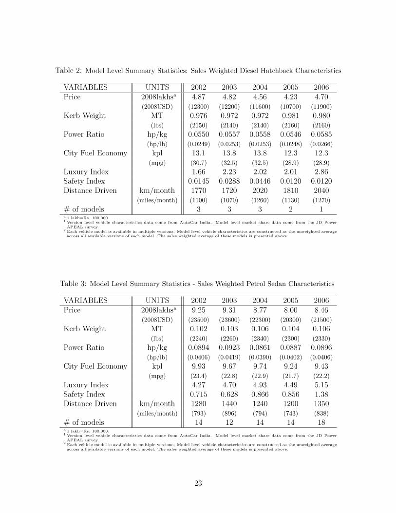
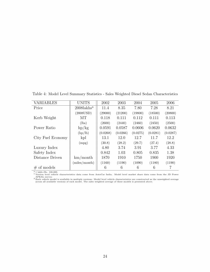
Tables 1-4 provide sales weighted summary statistics for prices and vehicle characteristics

for hatchbacks and sedans. Comparing this information with data on US vehicle characteris-

tics, from the United States Environmental Protection Agency, suggests that Indian cars are

lighter and less powerful in terms of power to weight ratio than cars in the US. In 2006, for

example, the sales weighted average weight of a vehicle purchased in India was about 1800

pounds for a hatchback and 2300 pounds for a sedan. In contrast, in the US, the average car

weighed approximately 3500 pounds (Environmental Protection Agency 2008). In the same

year, the average power to weight ratio (in horsepower per pound) was 0.032 for an Indian

hatchback, 0.041 for an Indian sedan and 0.054 for an average car in the US. In view of

their lighter weight and lower power ratio, it is perhaps not surprising that the average fuel

economy of the Indian hatchback and sedan (28.3 and 22.3 miles per gallon in city driving,

respectively)was greater than that of the average US car (19.4 miles per gallon).5 Estimates

of fuel economy technical frontiers (shown only for Indian cars in Table 8), however, suggest

that Indian cars are not necessarily as fuel efficient as US cars, holding weight and power

constant.6

5The figures for the US are the adjusted city miles per gallon rather than laboratory results, as reportedin USEPA (2008, Table 1).

6When the average US car is put through a fuel economy technical frontier similar to that reported inTable 7, its predicted fuel economy is less than 16 miles per gallon.

5

Comparisons of the sales weighted average petrol hatchback with the sales weighted

average diesel hatchback suggest that the diesel hatchbacks are heavier and less powerful

than their petrol counterparts. The same is true for sedans. These differences in vehicle

characteristics make it difficult to compare fuel economy by fuel type. In 2006, for example,

the sales weighted average fuel economy of the diesel sedan was 28.80 miles per gallon; its

petrol counterpart had a fuel economy of only 22.19 miles per gallon. Fuel economy for 2006

hatchbacks do not show such dramatic difference in fuel economy by fuel type. The diesel

hatchback had a fuel economy of 28.86 miles per gallon while that of the petrol hatchback was

28.43 miles per gallon; however, diesel hatchbacks were much heavier than petrol hatchbacks.

Tables 1-4 also show the average list price and distance driven of the four vehicle types.

Diesel hatchbacks are, on average, more expensive than petrol hatchbacks. Diesel sedans

were more expensive than petrol sedans in 2002. In the years 2003 to 2006, however, diesel

sedans were less expensive than petrol sedans. This reversal in the relative price for petrol

and diesel sedans can be attributed to the introduction of the relatively cheap and instantly

popular Tata Indigo in 2003. Additionally, owners of diesel vehicles appear to drive more each

month, irrespective of body type. Diesel hatchback owners drive approximately 75% more

than petrol hatchback owners per month while diesel sedan owners drive approximately 43%

more per month than petrol sedan owners. Furthermore, on average, sedan owners appear

to drive 22% more than hatchback owners.

3 Theoretical Framework

Break Even Period Analysis

Our first approach to evaluating consumer rationality asks whether it would be cheaper for

the buyer of petrol (diesel) vehicle to own and operate an otherwise identical vehicle in diesel

(petrol) form. If the buyer maximizes utility as described below, it would be irrational for

him to own a petrol vehicle if the otherwise identical diesel vehicle were cheaper. Formally,

6

we assume that the consumer selects the vector of vehicle characteristics (Z) to buy, miles

to drive (K) and fuel type (d) to maximize his utility, which is additively separable in the

utility of the chosen vehicle u(Z,K) and all other goods (x),

maxx,Z,K,d

U(x, Z,K) = x+ u(Z,K) (1)

The vector of vehicle characteristics (Z) includes weight, power, automatic transmission

and so forth. Fuel type (d) does not enter the utility function, but enters the consumer’s

budget constraint through its effect on vehicle price, P (Z, d), fuel price (denoted pd for diesel

and pp for petrol) and fuel economy (kpl),

y = x+ P (Z, d) +KT∑t=0

1

(1 + r)tdpd(t) + (1 − d)pp(t)

kpl(Z, d)(2)

In equation (2) y denotes wealth, r the discount rate, and T the expected life of the vehicle.

In solving this problem the consumer computes the optimal x, Z, and K conditional on his

choice of fuel type (d = 0 for petrol and d = 1 for diesel). The fuel type that yields the

highest utility is then chosen.

Using ∗’s to denote the optimal choice of vehicle characteristics and miles driven, we can

say that the buyer of a petrol vehicle is irrational if his chosen (Z∗p , K∗p) bundle is cheaper

in diesel form,

P (Z∗p , 0) +K∗p

T∑t=0

1

(1 + r)tpp(t)

kpl(Z∗P , 0)> P (Z∗p , 1) +K∗p

T∑t=0

1

(1 + r)tpd(t)

kpl(Z∗P , 1)(3)

This is simply to say that, all else equal, cheaper is better. If the same (Z∗p, K∗p) bundle

can be purchased more cheaply in diesel form, the consumer is not choosing optimally. (A

similar statement can obviously be made for diesel buyers.) Calculation of (3) requires that

we predict the price and fuel economy of the Z∗p vector of characteristics as a diesel vehicle.

Implementing this test of rationality requires estimating an hedonic price function to predict

7

vehicle prices and a fuel economy frontier to predict kilometers per liter as a function of Z

and d. Both the hedonic price function and the fuel economy frontier are described in section

4.

An equivalent way to calculate the rationality of petrol car buyers is to calculate the

break even period T̂ that would make the additional cost of Z∗p in diesel form equal to the

PDV of fuel savings,

P (Z∗p , 1) − P (Z∗p , 0) = K∗p

T̂∑t=0

1

(1 + r)t

(pp(t)

kpl(Z∗p , 0)− pd(t)

kpl(Z∗p , 1)

)(4)

and compare T̂ to T . T̂ < T suggests that the petrol car buyer is irrational. For the owner

of a diesel vehicle T̂ would be calculated analogously, but using the (Z∗d , K∗d) vector. Since

T̂ in both cases is the time required for the accumulated operating cost savings from a diesel

vehicle to cover the difference in purchase price, for a diesel owner, T̂ > T would indicate

irrationality. Equivalently, we could calculate the discount rate r′ that would make the break

even period T̂ equal to the life of the vehicle. An r′ value that exceeds the market interest

rate would also indicate consumer myopia.7

As in the literature on consumer purchases of energy efficient appliances, a high discount

rate may represent lack of information (e.g., people may not be well informed about differ-

ences in fuel economy across vehicles), failure to compare the difference in purchase price

to the difference in operating costs over the life of the vehicle, or lack of access to credit

markets. We are able, indirectly, to test whether consumers are poorly informed about fuel

economy across vehicles by comparing fuel economy estimates provided by new car buyers

(available through the J.D. Power APEAL survey) with estimates of fuel economy reported

in AutoCar India, an Indian car magazine that uses test runs to estimate fuel economy. As

for credit markets, they appear to be well functioning; over 70% of new cars in India are

7Note that our definition of rationality treats the purchaser in equations (1) and (2) as the sole ownerof the vehicle. Rationality thus assumes that both the new and used car markets operate efficiently. Analternative would be to evaluate the rationality of new car buyers, conditional on prices in the used carmarket. Data on the used car market in India are, however, not readily available.

8

financed by auto loans at an average interest rate of 12 − 14%.8

Willingness To Pay Analysis

One problem with the above rationality test is that it assumes that the chosen Z vector for

a petrol car is available in diesel form, and vice versa. This is not always true. Figures 7-16

show bundles of vehicle characteristics available in the market for hatchbacks and for sedans

for the model years 2002-2006. The dark dots represent available petrol models while the

grey dots represent diesel models. For the first test of rationality to be valid, there need to be

diesel bundles close to petrol bundles. This appears to hold for sedans, but not necessarily

for hatchbacks. This casts doubts on the validity of our break even analysis for petrol car

owners, especially hatchback owners. We therefore compare the cost of the chosen petrol

vehicle with the cost of the average diesel vehicle, i.e., with what is purchased in the market,

rather than with the otherwise identical diesel vehicle.

Our second rationality test compares the purchase price and operating costs of the chosen

petrol vehicle with the purchase price and operating costs of the average diesel vehicle sold.

Let x∗ denote the income remaining after the petrol car buyer purchases Z∗p and drives K∗p .

Let x′ denote the income remaining if he drives K∗p kilometers but purchases Z ′d, the vector

of characteristics of the average diesel vehicle. If the buyer is rational he prefers (x∗, Z∗p , K∗p)

to (x′, Z ′d, K∗p),

U(x∗, Z∗p , K∗p) > U(x′, Z ′d, K

∗p) (5)

However, there is some amount of money, x̂, that would make the buyer as happy with the

average diesel vehicle as with his chosen car,

U(x∗, Z∗p , K∗p) = U(x̂, Z ′d, K

∗p) (6)

8http://www.rupeetimes.com/news/car_loans/auto_loan_interest_rates_

slashed_by_bank_of_india_1079.html http://www.financialexpress.com/news/

auto-lenders-set-to-revise-interest-rates/407419/ http://www.carazoo.com/article/

1606200801/Car-Loans---More-Than-Meets-the-Eye

9

His willingness to pay for his chosen car above what he is willing to pay for the alternative

car is thus x̂− x∗. Since x̂ > x′, the buyer’s willingness to pay for Z∗p must be greater than

x′− x∗. The latter is the difference between the cost of buying and operating his chosen car

minus the cost of buying and operating the average diesel vehicle,

P (Z∗p , 0) − P (Z ′d, 1) +K∗p

T∑t=0

1

(1 + r)t

(pp(t)

kpl(Z∗p , 0)− pd(t)

kpl(Z ′d, 1)

)(7)

It is difficult to say how large (7) must be for a petrol car buyer to be irrational.9 What

x̂−x∗ in fact measures is the petrol car buyers preferences for his chosen vehicle rather than

a more fuel efficient, but less powerful, diesel vehicle.

4 Data and Estimation

We perform the rationality tests described in the previous section using data on vehicle sales

and kilometers driven from the J.D. Power APEAL survey, an annual survey of new car

buyers in India.10 This data set provides information on market share by model and fuel

type as well as buyer characteristics such as distance driven, income, and education level.

We compute separate measures for hatchback and sedan owners, and compute each measure

for the model years 2002 through 2006.

In computing the break even period for (e.g.) petrol hatchbacks we use the sales-weighted

vector of characteristics of petrol hatchbacks (for each model year) to estimate Z∗p . The char-

acteristics, which are described more fully below come from AutoCar India and Carwale.com.

K∗p is the average kilometers driven by owners of petrol hatchbacks in each model year. The

price of Z∗p as a diesel vehicle—and as a petrol vehicle—is calculated from the hedonic price

9A similar expression could be computed for the purchasers of diesel vehicles. We compute equation (7)only for petrol car buyers since the assumptions underlying counterfactual break even analysis are satisfiedfor diesel car buyers.

10The APEAL survey covers 5, 500 new car buyers each year. We have data on the percent of buyerspurchasing each model for each of the years 2002-2006. Summary statistics describing the buyers of eachmodel are also provided; however we did not have access to individual buyer data.

10

function for hatchbacks, described below. The fuel economy of Z∗p (in petrol form and diesel

form) is calculated from our estimated fuel economy frontier for hatchbacks, also described

below. Calculation of the break even period also requires estimates of petrol and diesel prices

over the life of the vehicle. We assume that fuel prices are equal to those observed in the

year of purchase. We use discount rates of 10% and 15% on the grounds that the average

interest rate on a new car loan in India is approximately 12 to 14%.

Estimates of how much more a petrol hatchback owner is willing to pay to drive his car

as a petrol rather than as a diesel vehicle require comparing the cost of Z∗p in petrol form,

P (Z∗p , 0), with the cost of Z∗p in diesel form, P (Z∗p , 1). All price and fuel economy estimates

are based on the hedonic price and fuel economy frontiers described in the next section. In

computing equation (7), T , the life of the vehicle, is assumed to be 11 years for hatchbacks

and 12 years for sedans (Rogers 2009).

Estimates of Hedonic Price and Fuel Economy Frontiers

To compute the purchase price of a (Z, d) vector, we estimate a semi-log hedonic price

function for the jtℎ vehicle of the form

logP (Zj, dj) =n∑

i=1

�izij + �dj + �j (8)

where d is the diesel indicator variable, equal to 1 for diesel and 0 for petrol.11 The tech-

nical frontier is estimated using the same list of vehicle characteristics, according to the

specification

log kpl(Zj, dj) =n∑

i=1

�izij + �dj + �j (9)

In order to avoid the problems of multicollinearity frequently reported in previous hedonic

price function analyses, we restrict the use of explanatory variables to a parsimonious list.

11Alternatively the equation logP (Zj , dj) =∑n

i=1 �izij + idjzij + �dj + �j could be used in place ofequation 8. Inclusion of these diesel interaction terms leads to loss of statistical significance which complicatesthe simulation and analysis of counterfactuals.

11

The variables included are chosen based on precedent in the literature and their link to

desirable vehicle properties (Atkinson and Halvorsen 1984; Ohta and Griliches 1986; Dreyfus

and Viscusi 1995; Espey and Nair 2005). To capture the many facets of luxury and safety,

two index variables are constructed as described below.

The key variables in our analysis are:

∙ Price - list price of vehicle in Delhi converted to January 2008 lakhs (100, 000 rupees)

using the urban non-manual worker CPI

∙ Kerb Weight - mass of vehicle in metric tons

∙ City Fuel Economy - fuel economy under urban driving conditions in kilometers

per litre

∙ Power Ratio - ratio of power (in horsepower) to kerbweight. This variable is a key

indicator of vehicle performance.

∙ Luxury Index - the sum of the indicator variables for air conditioning, power steering,

central locking, power windows, alloy wheels, leather seat, power mirrors, cd player,

and Carwale.com luxury rating (0-none, 1-luxury, or 2-super luxury)

∙ Safety Index - the sum of the indicator variables for airbags, rear seat belts, anti-lock

braking system, and traction control

∙ Automatic - an indicator variable for transmission type (0-manual or 1-automatic)

∙ Diesel - an indicator variable for fuel type (0-petrol or 1-diesel)

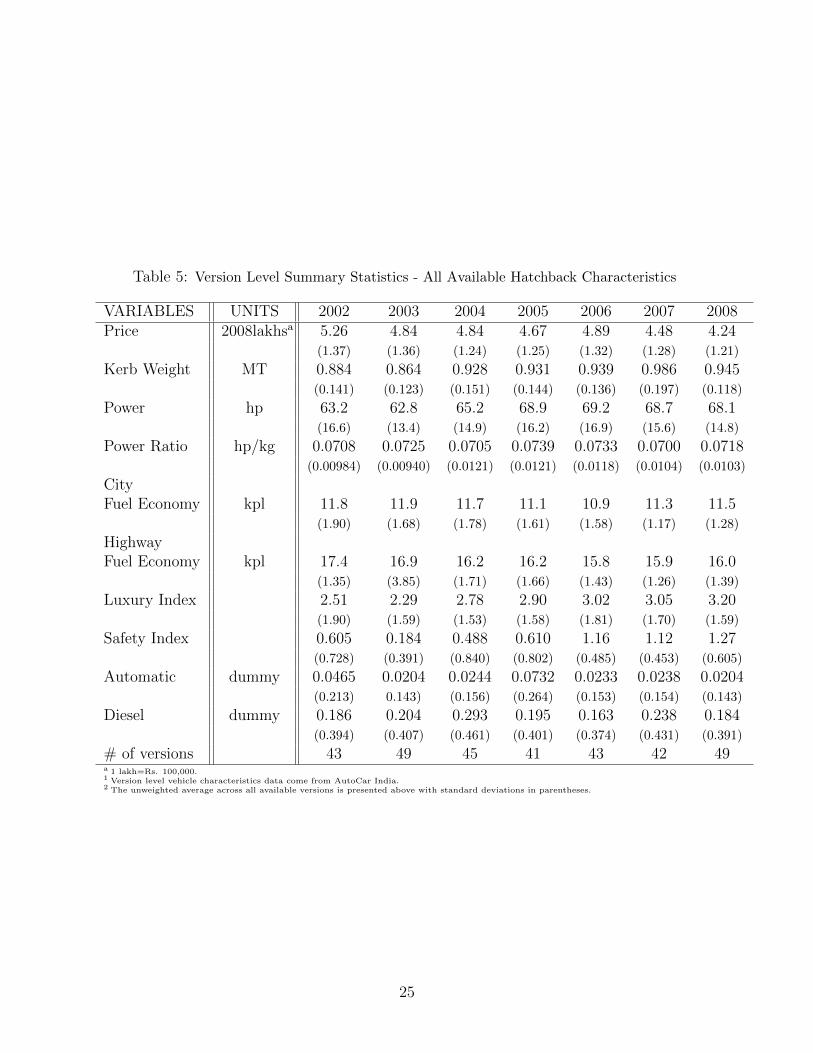
Tables 5 and 6 summarize the means and standard deviations of each variable, by model

year, for hatchbacks and sedans. Note that in estimating hedonic price functions and fuel

economy equations we use data on all models that appeared in AutoCar India, unweighted

by sales.

12

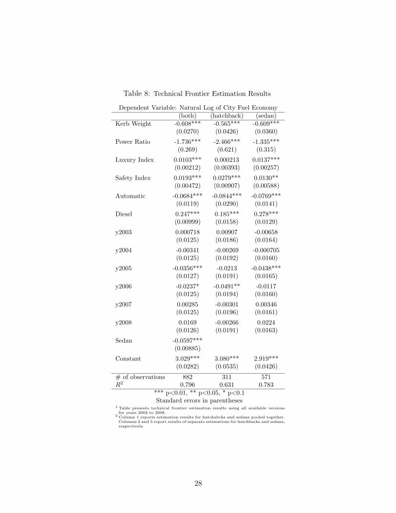
The hedonic price functions and fuel economy technical frontier estimation results are

presented in Tables 7 and 8. In both tables, column 1 includes both hatchbacks and sedans,

column 2 includes hatchbacks only, and column 3 includes sedans only. From columns 2

and 3 of Table 7 it appears that choosing diesel over petrol results in an approximately

15% increase in vehicle price for hatchbacks and an approximately 19% increase for sedans.

Similarly, diesel hatchbacks appear to be 19% more fuel efficient than petrol hatchbacks,

while diesel sedans are 28% more efficient (see Table 8).

In addition to the effects of fuel type on purchase price and fuel economy, several results

are worthy of remark. Almost all coefficients in Table 7, except for those on safetyindex

and the y2003 indicator variable in column 3, are statistically significant with signs that

agree with our expectations. Vehicle price varies positively with weight, power ratio, luxury,

automatic transmission (relative to standard), and diesel fuel type (relative to petrol). Safety

index has a positive and statistically significant coefficient when hatchbacks and sedans

are pooled, though not when the hedonic price function is estimated for each separately.

Additionally, year dummies indicate a nearly monotonic decline in quality adjusted purchase

price: holding the various vehicle characteristics constant, vehicles are becoming cheaper.

It should be noted, however, that vehicle characteristics are likely not being held constant.

Thus the quality adjusted drop in purchase price may not translate into lower unadjusted

prices.

As shown in Table 8 fuel economy decreases with vehicle weight, power to weight ratio,

and automatic transmission. Diesel cars have significantly higher fuel economy than petrol

cars, holding other characteristics constant. Fuel economy also varies positively with lux-

uryindex and safetyindex, though these coefficients are not always statistically significant

and are not substantial in magnitude. Year dummy coefficients are generally negative, but

rarely statistically significant and exhibit no clear time trend. The results of column 1 show

that sedans, all else equal, are approximately 6% less fuel efficient than their hatchback

counterparts.

13

5 Results on Fuel Economy and Vehicle Choice

Break Even Period Analysis

Tables 9 to 12 summarize the results of the break even analysis for owners of petrol hatch-

backs, diesel hatchbacks, petrol sedans, and diesel sedans. In each table the characteristics of

the “chosen” vehicle are the sales-weighted vehicle characteristics for that vehicle segment.

The regression results in Tables 7 and 8 are used to predict the price and fuel economy for

both the segment representative vehicle (the chosen vehicle) and the counterfactual vehicle,

in which only fuel type has been switched. The break even period is presented for each

model year using 10% and 15% discount rates .

The break even period for owners of diesel vehicles (both hatchbacks and sedans) is always

lower than the life of the vehicle, suggesting that buyers of diesel vehicles are indeed rational.

For owners of diesel hatchbacks, the break even period is between 1.5 and 2.5 years. This

is the outcome of a modest price premium for a diesel hatchback (about 70, 000 rupees) but

fuel savings of 3, 000-4, 000 rupees per month. Because the fuel cost savings from driving

a diesel hatchback are increasing over time the break even period is falling over time. The

break even period for owners of diesel sedans varies between 5.2 and 2.7 years, and is also

falling over time. This is due both to rising fuel cost savings and a narrowing of the spread

between the price of the average diesel sedan and its counterfactual petrol counterpart.

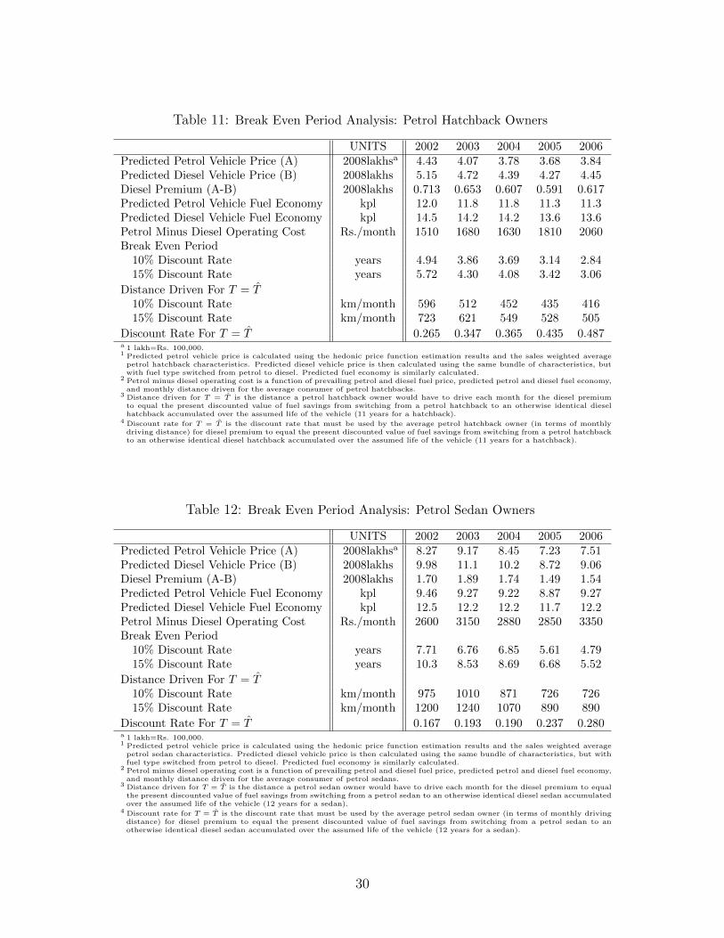
If drivers of petrol cars are rational, their break even period—the length of time it takes

a diesel version of their car to pay for itself—should be greater than the expected life of

their car. This does not appear to be the case for owners of either petrol hatchbacks or

sedans. Although data on vehicle life in India is scarce, Rogers(2009) suggests that the

median lifetime of a small car is between 11 and 12 years, while it is between 12 and 13

years for a medium-sized car. In contrast, the break even period ranges from 3 to 6 years

for petrol hatchbacks and from 5 to 10 years for petrol sedans. The break even period for

owners of petrol hatchbacks is longer than for owners of diesel hatchbacks since owners of

14

petrol hatchbacks, on average, drive fewer miles than diesel hatchback owners. The initial

price premium for a diesel hatchback, however, still pays for itself in less than 6 years. The

longer break even period for petrol sedans reflects the substantial price premium for a diesel

sedan (between 150, 000 and 170, 000 rupees). For both petrol hatchbacks and sedans length

of the payback period is falling over time. As above, this is due to an increase in the price

of petrol and diesel fuel and a decreasing diesel price premium.12

Because the time it takes a diesel vehicle to pay for itself in fuel savings is falling over

time for both diesel hatchbacks and diesel sedans, we would expect the market share of

diesel vehicles to be increasing for each segment.13 This is indeed true for sedans, but not

for hatchbacks. As Figure 6 shows, diesel sedan sales rose from 11% of the sedan market in

2002 to 33% in 2006. In contrast, the diesel share of hatchback sales remained approximately

constant at 15% over this period (see Figure 5). Indeed, by 2006 only one diesel hatchback,

the Tata Indica, had positive market share. We discuss this point further below.

Heterogeneity and Myopia in the Car Market

The preceding results suggest that more buyers of petrol cars should be switching to diesel;

however, the break even analysis is based on the mean number of kilometers driven by owners

of petrol hatchbacks and sedans. Buyers who drive fewer kilometers may well be rational.

Tables 11 and 12 also report the maximum number of kilometers that the owner of a petrol

hatchback or sedan could drive each year and have a break even period that equals the life of

the car. These numbers are much smaller than mean distance driven, and generally decrease

with each model year. In 2006 a petrol car driver who buys the sales-weighted average

petrol hatchback would have to drive no more than 500 km (approximately 300 miles) each

month for the purchase of the petrol hatchback to be rational—less than half of the mean

12This analysis assumes that the maintenance costs of diesel and petrol vehicles are the same. If mainte-nance costs are higher for diesel vehicles, this would increase the break even period.

13Formally, the probability of purchasing a diesel vehicle, is an increasing function of the difference inutility between the optimal diesel vehicle and the optimal petrol vehicle. The latter is an increasing functionof the difference in operating costs between the two vehicles, and a decreasing function of the difference inpurchase price.

15

distance driven (1140 km). For owners of petrol sedans the maximum K is approximately

900 km, compared to a mean distance of 1350 km. Unfortunately, we do not have data

on the distribution of monthly distance driven by vehicle type, which would enable us to

estimate the fraction of buyers who fail the rationality test.

Another way to present the results of our first rationality test is to calculate the discount

rate that would make the break even period equal the life of the car. This is presented

in Tables 11 and 12 for the owners of petrol hatchbacks and sedans who drive the mean

distance traveled. As expected, given the declining break even period, the discount rate r′

is increasing over time; for petrol hatchbacks the rate increases from 27% in 2002 to 49% in

2006 while for petrol sedans the increase over the same period is 17% to 28%. Given that

the average interest rate on a new car loan is between 12 and 14%, these discount rates are

high.

In the literature on the purchase of energy efficient appliances (Hausman 1979; Jaffe,

Newell, and Stavins 2003) high discount rates are interpreted as reflecting either lack of

information on the part of buyers, failure to take this information into account when making

purchases, or market failure. The latter can include failure of capital markets (buyers can’t

borrow to cover the cost of more energy efficient appliances) or agency problems—home

buyers fail to install such appliances because they believe that the housing market does not

fully price their benefits.

In the case of the Indian car market we can speak to the first issue by comparing owners’

assessments of fuel economy with figures published by AutoCar India on city and highway

kilometers per liter. The two sets of figures agree very well. A regression through the origin

of buyers’ estimates of fuel economy on published estimates of city fuel economy yields a

coefficient of 0.83 (s.e. = .0087); when highway fuel economy is added to the equation,

the coefficient on city fuel economy equals 1.00 (s.e. = .10) and the coefficient on highway

fuel economy is 0.12 (s.e. = .078). Buyers’ assessments of fuel economy agree very well

with published figures, and consequently, high discount rates for petrol vehicles cannot be

16

explained by a lack of information on fuel economy.

As for the question of market failure, high discount rates do not appear to be driven by

a lack of credit. Over 70% of new car purchases are fincanced by auto loans, with interest

rates ranging from 12 to 14% (see footnote 8). Lack of data on the secondary market for

passenger vehicles prevents us from evaluating whether the high discount rate is driven by

the failure of the used car market to fully price fuel economy.

On the basis of the analysis in this and the previous section, can we conclude that

purchasers of petrol hatchbacks and sedans are irrational, at least those purchasers driving

distances above the maximum K? This conclusion would be warranted if it were the case

that petrol car owners could in fact purchase otherwise identical diesel vehicles. The next

section explores whether this assumption is true.

Willingness To Pay Analysis

The preceding analysis assumes that buyers of petrol hatchbacks and sedans could buy their

chosen car as an otherwise identical diesel vehicle in which only the fuel type has been

changed. To examine whether this is the case we plot bundles of vehicle characteristics

available in the diesel market on graphs showing the mean sales-weighted characteristics of

the chosen petrol hatchback and chosen petrol sedan for each model year (Figures 7-16). A

comparison of available bundles of characteristics for diesel and petrol hatchbacks in Figures

7-11 shows that very few hatchbacks are available in diesel form. As for sedans, there appear

to be close substitutes for some, but not all, models. This suggests the possibility that

petrol hatchback and sedan owners are not irrational but are placing a high premium on

other vehicle characteristics than fuel economy.

To explore this possibility further we calculate the difference in purchase price plus op-

erating costs between the chosen petrol vehicle and the average diesel vehicle sold in each

year. This difference (equation 7) represents the present value of the money a petrol car

owner forgoes by not buying a diesel car and, as argued in section 3, is a lower bound to his

17

willingness to pay to own his chosen petrol vehicle above what he is willing to pay for the

average diesel alternative.

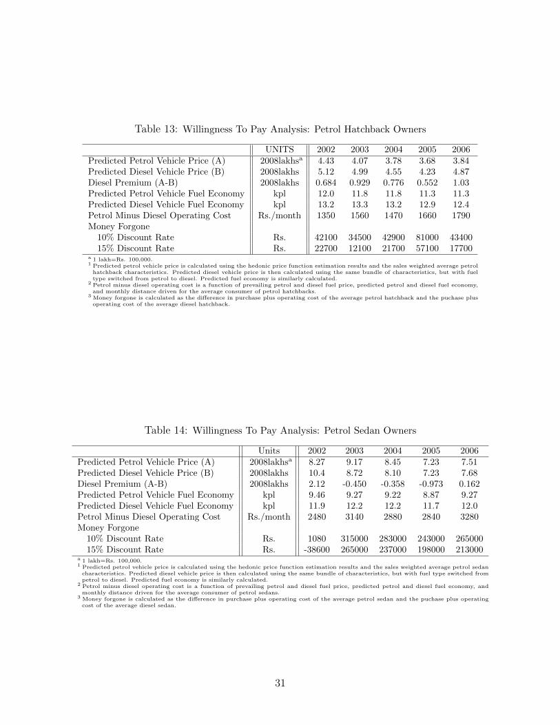
As Table 13 shows, the money a petrol hatchback owner forgoes by not buying the

average diesel fluctuates across the 2002 to 2006 model years. It averages Rs. 49, 000 at a

10% discount rate and Rs. 26, 000 at a 15% discount rate. These amounts are approximately

10% and 5% of the cost of a new petrol hatchback. The amounts are lower bounds to what

the owner is willing to pay for a more powerful, but less fuel efficient vehicle above what he

is willing to pay for the average diesel alternative.

The situation is somewhat different for owners of petrol sedans. The lower bound to

what they are willing to pay for a more powerful, but less fuel efficient vehicle, is much

larger in absolute terms than what hatchback owners are willing to pay, and much larger

relative to the purchase price of the car. These amounts are shown in Table 14. The drastic

change between the years 2002 and 2003 is explained by the 2003 introduction of the Tata

Indigo, a low price sedan that captured approximately 60% of the diesel sedan market and

approximately 7% of the petrol sedan market. By drastically lowering the purchase price of

the average diesel sedan, this model increased the difference in purchase price plus operating

cost between the chosen petrol sedan and the average diesel sedan. Focusing on the period

2003 to 2006, the lower bound to the difference in what sedan owners will pay for a more

powerful but less fuel efficient car (relative to what they are willing to pay for the average

diesel alternative) ranges from Rs. 198, 000 to Rs. 265, 000 (or about 27% of the cost of the

car) using a 15% discount rate.

6 Summary And Conclusions

One justification for fuel economy regulation is consumer myopia. If consumers fail to ap-

preciate the cost savings associated with buying a more fuel efficient vehicle or, equivalently,

if they discount them at a higher rate than they exhibit in other markets, fuel economy

18

standards may be warranted. We have attempted to address this question by calculating

the length of time it would take for the fuel savings associated with a diesel vehicle to just

equal the additional purchase price of the vehicle, compared with an identical petrol vehicle

(i.e., the break even period). If buyers consider fuel savings rationally, this period should be

shorter than the life of the vehicle for owners of diesel vehicles; for owners of petrol vehicles

it should be longer. We have also calculated the discount rate that makes the break even

period equal to the life of the vehicle for buyers of diesel and petrol vehicles.

Using a 10% or 15% discount rate, the owner of the average diesel car indeed seems

rational. The break even period for the model years 2002 to 2006 is between 1.5 and 2.5

years for diesel hatchback owners and between 2.5 and 5.2 years for diesel sedan owners. The

break even period has been falling over time, due largely to increases in the spread between

the cost per kilometer of driving a petrol and a diesel vehicle.

Similar calculations for owners of petrol vehicles suggest that they are myopic. People

who buy petrol vehicles have longer break even periods (partly because they drive fewer

kilometers per year than diesel owners), but these periods are shorter than average vehicle

life. At a 15% discount rate they range between 3.1 and 5.7 years for hatchback owners and

5.5 and 10 years for owners of petrol sedans, compared to median vehicle lives of 11 and 12

years, respectively. Equivalently, the discount rates that equate the break even period to

the life of the vehicle in 2006 are 49% for petrol hatchback owners and 28% for petrol sedan

owners.

We note that this apparent myopia is not the result of Indian car owners failing to

appreciate differences in fuel economy among vehicles. When an owner’s assessment of fuel

economy from the J.D. Power APEAL survey is regressed on published fuel economy data

from AutoCar India, the two are in very close agreement. It is, however, the case that the

assumption underlying our calculations—that the buyer of a petrol vehicle can purchase

an identical vehicle (in terms of power weight ratio, vehicle weight, etc.) in diesel form—

may not be true. Buyers of petrol vehicles may indeed have to sacrifice power (and other

19

characteristics) when they switch to the diesel version of their car.

This leads us construct an alternate test of the rationality of petrol car buyers in which we

calculate the difference in the purchase price-plus-present value of operating costs between

the chosen petrol vehicle and the average diesel vehicle sold each year. This is a lower bound

to what a petrol buyer is willing to pay (above his willingness to pay for the average diesel

car) for his more powerful, but more costly to operate, petrol car. Averaged across the 2002-

2006 model years, this amount for hatchback owners is approximately Rs. 49, 000 using a

10% discount rate and Rs. 26, 000 at a discount rate of 15%. These amounts are lower

bounds to willingness to pay, but are a small fraction of the purchase price of a hatchback

(approximately Rs. 400, 000). Sedan owners are willing to pay a much higher amount in

absolute and relative terms to own a more powerful but less fuel efficient vehicle. At a

15% discount rate they are willing to pay at least 25% of the car’s purchase price (over Rs.

200, 000); at a 10% discount rate this amount increases to approximately 30% of the cost of

a petrol sedan (over Rs. 220, 000) for model years 2003-2006.

We cannot, however, conclude from this information that buyers of petrol cars are nec-

essarily myopic. They may simply place a high premium on power and other characteristics

that would be lacking in the average diesel car. These preferences must be taken into account

in evaluating the desirability of fuel economy standards. If, for example, auto manufacturers

in India were to meet fuel economy standards by reducing vehicle weight and power, as was

done in the U.S. (Klier and Linn 2008), this could result in a welfare loss to Indian con-

sumers that would have to be balanced against the gains (e.g., to national security) from

reducing dependence on foreign oil. Evaluating these tradeoffs requires estimating the struc-

tural model in equations (1) and (2), as well as modeling the supply side of the market. We

are currently estimating a structural model of consumer choice using the data from the J.D.

Power APEAL survey. This will allow us to examine the welfare implications of alternative

forms of fuel economy regulation, including the possibility of removing the subsidy to diesel

fuel.

20

References

Atkinson, S. E. and R. Halvorsen (1984). A new hedonic technique for estimating at-tribute demand: An application to the demand for automobile efficiency. The Reviewof Economics and Statistics 66 (3), 417–426.

Austin, D. and T. Dinan (2005). Clearing the air: The costs and consequences of highercafe standards and increased gasoline taxes. Journal of Environmental Economics andManagement 50, 562–582.

Dreyfus, M. K. and W. K. Viscusi (1995). Rates of time preference and consumer val-uations of automobile safety and fuel efficiency. Journal of Law and Economics 38,79–105.

Environmental Protection Agency (2008). Light-Duty Automotive Technology and FuelEconomy Trends: 1975 Through 2008. Office of Transportation and Air Quality.

Espey, M. and S. Nair (2005). Automobile fuel economy: What is it worth? ContemporaryEconomic Policy 23 (3), 317–323.

Hausman, J. (1979). Individual discount rates and the purchase and utilization of energy-using durables. Bell Journal of Economics 10 (1), 33–54.

Jacobsen, M. (2008). Evaluating fuel efficiency standards in a model with producerand household heterogeneity. Working Paper , Available online at econ.ucsd.edu/

˜m3jacobs.

Jaffe, A. B., R. G. Newell, and R. N. Stavins (2003). Chapter 11 technological change andthe environment. In K. G. Mler and J. R. Vincent (Eds.), Handbook of EnvironmentalEconomics, Volume 1 of Handbook of Environmental Economics, Chapter 11, pp. 461–516. Elsevier.

Klier, T. and J. Linn (2008). New vehicle characteristics and the cost of the corporateaverage fuel economy standard. Working Paper Series WP-08-13.

Ohta, M. and Z. Griliches (1986). Automobile prices and quality: Did the gasoline priceincrease change consumer tastes in the u.s.? Journal of Business & Economic Statis-tics 4 (2), 187–198.

Parry, I. W. H., M. Walls, and W. Harrington (2007). Automobile externalities and poli-cies. Journal of Economic Literature 45, 373–399.

Portney, P. R., I. W. H. Parry, H. K. Gruenspecht, and W. Harrington (2003). Theeconomics of fuel economy. Journal of Economic Perspectives 17 (4), 203–217.

Rogers, J. A. (2009). personal communication.

21

Table 1: Model Level Summary Statistics: Sales Weighted Petrol Hatchback Characteristics

VARIABLES UNITS 2002 2003 2004 2005 2006Price 2008lakhsa 4.72 4.06 4.00 3.72 3.96

(2008 USD) (12000) (10300) (10100) (9450) (10000)

Kerb Weight MT 0.771 0.749 0.759 0.777 0.810(lbs) (1700) (1650) (1670) (1710) (1790)

Power Ratio hp/kg 0.0698 0.0732 0.0684 0.0713 0.0707(hp/lb) (0.0317) (0.0332) (0.0310) (0.0324) (0.0321)

City Fuel Economy kpl 12.4 12.3 11.9 12.0 12.1(mpg) (29.1) (29.0) (27.9) (28.2) (28.4)

Luxury Index 2.37 1.67 2.07 1.92 2.17Safety Index 0.657 0.0224 0.0562 0.156 1.25Distance Driven km/month 1030 1080 990 1090 1140

(miles/month) (641) (670) (615) (678) (708)

# of models 9 7 8 10 9a 1 lakh=Rs. 100,000.1 Version level vehicle characteristics data come from AutoCar India. Model level market share data come from the JD Power

APEAL survey.2 Each vehicle model is available in multiple versions. Model level vehicle characteristics are constructed as the unweighted average

across all available versions of each model. The sales weighted average of these models is presented above.

22

Table 2: Model Level Summary Statistics: Sales Weighted Diesel Hatchback Characteristics


(2008USD) (12300) (12200) (11600) (10700) (11900)





(miles/month) (1100) (1070) (1260) (1130) (1270)




Table 3: Model Level Summary Statistics - Sales Weighted Petrol Sedan Characteristics


(2008USD) (23500) (23600) (22300) (20300) (21500)





(miles/month) (793) (896) (794) (743) (838)




23

Table 4: Model Level Summary Statistics - Sales Weighted Diesel Sedan Characteristics


(2008USD) (29000) (21200) (19800) (18500) (20800)





(miles/month) (1160) (1190) (1090) (1180) (1190)




24

Table 5: Version Level Summary Statistics - All Available Hatchback Characteristics

VARIABLES UNITS 2002 2003 2004 2005 2006 2007 2008Price 2008lakhsa 5.26 4.84 4.84 4.67 4.89 4.48 4.24

(1.37) (1.36) (1.24) (1.25) (1.32) (1.28) (1.21)

Kerb Weight MT 0.884 0.864 0.928 0.931 0.939 0.986 0.945(0.141) (0.123) (0.151) (0.144) (0.136) (0.197) (0.118)

Power hp 63.2 62.8 65.2 68.9 69.2 68.7 68.1(16.6) (13.4) (14.9) (16.2) (16.9) (15.6) (14.8)

Power Ratio hp/kg 0.0708 0.0725 0.0705 0.0739 0.0733 0.0700 0.0718(0.00984) (0.00940) (0.0121) (0.0121) (0.0118) (0.0104) (0.0103)

CityFuel Economy kpl 11.8 11.9 11.7 11.1 10.9 11.3 11.5

(1.90) (1.68) (1.78) (1.61) (1.58) (1.17) (1.28)

HighwayFuel Economy kpl 17.4 16.9 16.2 16.2 15.8 15.9 16.0

(1.35) (3.85) (1.71) (1.66) (1.43) (1.26) (1.39)

Luxury Index 2.51 2.29 2.78 2.90 3.02 3.05 3.20(1.90) (1.59) (1.53) (1.58) (1.81) (1.70) (1.59)

Safety Index 0.605 0.184 0.488 0.610 1.16 1.12 1.27(0.728) (0.391) (0.840) (0.802) (0.485) (0.453) (0.605)

Automatic dummy 0.0465 0.0204 0.0244 0.0732 0.0233 0.0238 0.0204(0.213) 0.143) (0.156) (0.264) (0.153) (0.154) (0.143)

Diesel dummy 0.186 0.204 0.293 0.195 0.163 0.238 0.184(0.394) (0.407) (0.461) (0.401) (0.374) (0.431) (0.391)

# of versions 43 49 45 41 43 42 49a 1 lakh=Rs. 100,000.1 Version level vehicle characteristics data come from AutoCar India.2 The unweighted average across all available versions is presented above with standard deviations in parentheses.

25

Table 6: Version Level Summary statistics - All Available Sedan Characteristics

VARIABLES UNITS 2002 2003 2004 2005 2006 2007 2008Price 2008lakhsa 10.1 12.7 13.7 14.2 15.4 15.1 15.7

(4.48) (9.79) (14.7) (16.3) (16.9) (16.1) (15.3)

Kerb Weight MT 1.14 1.13 1.17 1.19 1.23 1.23 1.27(0.133) (0.188) (0.209) (0.218) (0.237) (0.209) (0.209)

Power hp 83.2 94.5 102 108 113 116 120(28.1) (29.2) (39.2) (43.6) (50.3) (49.1) (50.0)

Power Ratio hp/kg 0.0735 0.0831 0.0858 0.0887 0.0900 0.0915 0.0922(0.0225) (0.0172) (0.0189) (0.0216) (0.0240) (0.0232) (0.0237)

CityFuel Economy kpl 9.97 9.81 9.51 9.14 9.15 9.35 9.66

(1.57) (1.79) (2.03) (2.07) (2.00) (1.95) (2.09)

HighwayFuel Economy kpl 14.2 13.4 12.7 13.7 13.8 14.0 14.3

(2.83) (2.60) (2.87) (2.91) (2.95) (2.80) (2.92)

Luxury Index 4.09 5.25 5.44 5.73 6.09 6.30 6.83(2.69) (2.20) (2.40) (2.52) (2.37) (2.57) (2.42)

Safety Index 0.853 1.00 1.32 1.65 2.10 2.07 2.46(1.11) (1.40) (1.45) (1.49) (1.37) (1.20) (1.17)

Automatic dummy 0.0400 0.0556 0.152 0.230 0.247 0.270 0.304(0.197) 0.231) (0.361) (0.424) (0.434) (0.446) (0.463)

Diesel dummy 0.347 0.264 0.215 0.270 0.225 0.258 0.359(0.479) (0.444) (0.414) (0.447) (0.420) (0.440) (0.482)

# of versions 75 72 79 74 89 89 92a 1 lakh=Rs. 100,000.1 Version level vehicle characteristics data come from AutoCar India.2 The unweighted average across all available versions is presented above with standard deviations in parentheses.

26

Table 7: Hedonic Price Function Estimation Results

Dependent Variable: Natural Log of Price(both) (hatchback) (sedan)

Kerb Weight 1.329*** 0.837*** 1.497***(0.0398) (0.0471) (0.0514)

Power Ratio 8.416*** 8.544*** 7.948***(0.406) (0.679) (0.499)

Luxury Index 0.0695*** 0.0680*** 0.0758***(0.00378) (0.00432) (0.00493)

Safety Index 0.0138* -0.0147 0.00219(0.00810) (0.00987) (0.0104)

Automatic 0.218*** 0.182*** 0.165***(0.0199) (0.0249) (0.0256)

Diesel 0.177*** 0.149*** 0.187***(0.0173) (0.0172) (0.0232)

y2003 -0.00702 -0.0648*** 0.0166(0.0233) (0.0208) (0.0327)

y2004 -0.126*** -0.144*** -0.0976***(0.0231) (0.0208) (0.0320)

y2005 -0.220*** -0.215*** -0.207***(0.0234) (0.0215) (0.0322)

y2006 -0.228*** -0.165*** -0.235***(0.0230) (0.0215) (0.0314)

y2007 -0.290*** -0.275*** -0.269***(0.0230) (0.0217) (0.0315)

y2008 -0.334*** -0.309*** -0.327***(0.0227) (0.0210) (0.0312)

Sedan 0.128***(0.0154)

Constant -0.391*** 0.0842 -0.448***(0.0376) (0.0585) (0.0561)

# of observations 986 327 659R2 0.948 0.868 0.934

Standard errors in parentheses*** p<0.01, ** p<0.05, * p<0.1

1 Table presents hedonic price function estimation results using all available ver-sions for years 2002 to 2008.

2 Column 1 reports estimation results for hatchabcks and sedans pooled together.Columns 2 and 3 report results of separate estimations for hatchbacks andsedans, respectively.

27

Table 8: Technical Frontier Estimation Results

Dependent Variable: Natural Log of City Fuel Economy(both) (hatchback) (sedan)

Kerb Weight -0.608*** -0.565*** -0.609***(0.0270) (0.0426) (0.0360)

Power Ratio -1.736*** -2.466*** -1.335***(0.269) (0.621) (0.315)

Luxury Index 0.0103*** 0.000213 0.0137***(0.00212) (0.00393) (0.00257)

Safety Index 0.0193*** 0.0279*** 0.0130**(0.00472) (0.00907) (0.00588)

Automatic -0.0684*** -0.0844*** -0.0769***(0.0119) (0.0290) (0.0141)

Diesel 0.247*** 0.185*** 0.278***(0.00999) (0.0158) (0.0129)

y2003 0.000718 0.00907 -0.00658(0.0125) (0.0186) (0.0164)

y2004 -0.00341 -0.00269 -0.000705(0.0125) (0.0192) (0.0160)

y2005 -0.0356*** -0.0213 -0.0438***(0.0127) (0.0191) (0.0165)

y2006 -0.0237* -0.0491** -0.0117(0.0125) (0.0194) (0.0160)

y2007 0.00285 -0.00301 0.00346(0.0125) (0.0196) (0.0161)

y2008 0.0169 -0.00266 0.0224(0.0126) (0.0191) (0.0163)

Sedan -0.0597***(0.00885)

Constant 3.029*** 3.080*** 2.919***(0.0282) (0.0535) (0.0426)

# of observations 882 311 571R2 0.796 0.631 0.783

*** p<0.01, ** p<0.05, * p<0.1Standard errors in parentheses

1 Table presents technical frontier estimation results using all available versionsfor years 2002 to 2008.

2 Column 1 reports estimation results for hatchabcks and sedans pooled together.Columns 2 and 3 report results of separate estimations for hatchbacks and sedans,respectively.

28

Table 9: Break Even Period Analysis: Diesel Hatchback Owners

UNITS 2002 2003 2004 2005 2006Predicted Petrol Vehicle Price (A) 2008lakhsa 4.41 4.30 3.92 3.65 4.19Predicted Diesel Vehicle Price (B) 2008lakhs 5.12 4.99 4.55 4.23 4.87Diesel Premium (A-B) 2008lakhs 0.709 0.691 0.630 0.586 0.674Predicted Petrol Vehicle Fuel Economy kpl 11.0 11.1 10.9 10.7 10.3Predicted Diesel Vehicle Fuel Economy kpl 13.2 13.3 13.2 12.9 12.4Petrol Minus Diesel Operating Cost Rs./month 2830 2870 3580 3190 4050Break Even Period

10% Discount Rate years 2.32 2.23 1.58 1.65 1.4915% Discount Rate years 2.46 2.36 1.64 1.72 1.54

a 1 lakh=Rs. 100,000.1 Predicted diesel vehicle price is calculated using the hedonic price function estimation results and the sales weighted average

diesel hatchback characteristics. Predicted petrol vehicle price is then calculated using the same bundle of characteristics, butwith fuel type switched from diesel to petrol. Predicted fuel economy is similarly calculated.

2 Petrol minus diesel operating cost is a function of prevailing petrol and diesel fuel price, predicted petrol and diesel fuel economy,and monthly distance driven for the average consumer of diesel hatchbacks.

Table 10: Break Even Period Analysis: Diesel Sedan Owners



a 1 lakh=Rs. 100,000.1 Predicted diesel vehicle price is calculated using the hedonic price function estimation results and the sales weighted average

diesel sedan characteristics. Predicted petrol vehicle price is then calculated using the same bundle of characteristics, butwith fuel type switched from diesel to petrol. Predicted fuel economy is similarly calculated.

2 Petrol minus diesel operating cost is a function of prevailing petrol and diesel fuel price, predicted petrol and diesel fueleconomy, and monthly distance driven for the average consumer of diesel sedans.

29

Table 11: Break Even Period Analysis: Petrol Hatchback Owners



Distance Driven For T = T̂10% Discount Rate km/month 596 512 452 435 41615% Discount Rate km/month 723 621 549 528 505

Discount Rate For T = T̂ 0.265 0.347 0.365 0.435 0.487a 1 lakh=Rs. 100,000.1 Predicted petrol vehicle price is calculated using the hedonic price function estimation results and the sales weighted average

petrol hatchback characteristics. Predicted diesel vehicle price is then calculated using the same bundle of characteristics, butwith fuel type switched from petrol to diesel. Predicted fuel economy is similarly calculated.

2 Petrol minus diesel operating cost is a function of prevailing petrol and diesel fuel price, predicted petrol and diesel fuel economy,and monthly distance driven for the average consumer of petrol hatchbacks.

3 Distance driven for T = T̂ is the distance a petrol hatchback owner would have to drive each month for the diesel premiumto equal the present discounted value of fuel savings from switching from a petrol hatchback to an otherwise identical dieselhatchback accumulated over the assumed life of the vehicle (11 years for a hatchback).

4 Discount rate for T = T̂ is the discount rate that must be used by the average petrol hatchback owner (in terms of monthlydriving distance) for diesel premium to equal the present discounted value of fuel savings from switching from a petrol hatchbackto an otherwise identical diesel hatchback accumulated over the assumed life of the vehicle (11 years for a hatchback).

Table 12: Break Even Period Analysis: Petrol Sedan Owners



Distance Driven For T = T̂10% Discount Rate km/month 975 1010 871 726 72615% Discount Rate km/month 1200 1240 1070 890 890

Discount Rate For T = T̂ 0.167 0.193 0.190 0.237 0.280a 1 lakh=Rs. 100,000.1 Predicted petrol vehicle price is calculated using the hedonic price function estimation results and the sales weighted average

petrol sedan characteristics. Predicted diesel vehicle price is then calculated using the same bundle of characteristics, but withfuel type switched from petrol to diesel. Predicted fuel economy is similarly calculated.

2 Petrol minus diesel operating cost is a function of prevailing petrol and diesel fuel price, predicted petrol and diesel fuel economy,and monthly distance driven for the average consumer of petrol sedans.

3 Distance driven for T = T̂ is the distance a petrol sedan owner would have to drive each month for the diesel premium to equalthe present discounted value of fuel savings from switching from a petrol sedan to an otherwise identical diesel sedan accumulatedover the assumed life of the vehicle (12 years for a sedan).

4 Discount rate for T = T̂ is the discount rate that must be used by the average petrol sedan owner (in terms of monthly drivingdistance) for diesel premium to equal the present discounted value of fuel savings from switching from a petrol sedan to anotherwise identical diesel sedan accumulated over the assumed life of the vehicle (12 years for a sedan).

30

Table 13: Willingness To Pay Analysis: Petrol Hatchback Owners

UNITS 2002 2003 2004 2005 2006Predicted Petrol Vehicle Price (A) 2008lakhsa 4.43 4.07 3.78 3.68 3.84Predicted Diesel Vehicle Price (B) 2008lakhs 5.12 4.99 4.55 4.23 4.87Diesel Premium (A-B) 2008lakhs 0.684 0.929 0.776 0.552 1.03Predicted Petrol Vehicle Fuel Economy kpl 12.0 11.8 11.8 11.3 11.3Predicted Diesel Vehicle Fuel Economy kpl 13.2 13.3 13.2 12.9 12.4Petrol Minus Diesel Operating Cost Rs./month 1350 1560 1470 1660 1790Money Forgone

10% Discount Rate Rs. 42100 34500 42900 81000 4340015% Discount Rate Rs. 22700 12100 21700 57100 17700

a 1 lakh=Rs. 100,000.1 Predicted petrol vehicle price is calculated using the hedonic price function estimation results and the sales weighted average petrol

hatchback characteristics. Predicted diesel vehicle price is then calculated using the same bundle of characteristics, but with fueltype switched from petrol to diesel. Predicted fuel economy is similarly calculated.

2 Petrol minus diesel operating cost is a function of prevailing petrol and diesel fuel price, predicted petrol and diesel fuel economy,and monthly distance driven for the average consumer of petrol hatchbacks.

3 Money forgone is calculated as the difference in purchase plus operating cost of the average petrol hatchback and the puchase plusoperating cost of the average diesel hatchback.

Table 14: Willingness To Pay Analysis: Petrol Sedan Owners

Units 2002 2003 2004 2005 2006Predicted Petrol Vehicle Price (A) 2008lakhsa 8.27 9.17 8.45 7.23 7.51Predicted Diesel Vehicle Price (B) 2008lakhs 10.4 8.72 8.10 7.23 7.68Diesel Premium (A-B) 2008lakhs 2.12 -0.450 -0.358 -0.973 0.162Predicted Petrol Vehicle Fuel Economy kpl 9.46 9.27 9.22 8.87 9.27Predicted Diesel Vehicle Fuel Economy kpl 11.9 12.2 12.2 11.7 12.0Petrol Minus Diesel Operating Cost Rs./month 2480 3140 2880 2840 3280Money Forgone

10% Discount Rate Rs. 1080 315000 283000 243000 26500015% Discount Rate Rs. -38600 265000 237000 198000 213000

a 1 lakh=Rs. 100,000.1 Predicted petrol vehicle price is calculated using the hedonic price function estimation results and the sales weighted average petrol sedan

characteristics. Predicted diesel vehicle price is then calculated using the same bundle of characteristics, but with fuel type switched frompetrol to diesel. Predicted fuel economy is similarly calculated.

2 Petrol minus diesel operating cost is a function of prevailing petrol and diesel fuel price, predicted petrol and diesel fuel economy, andmonthly distance driven for the average consumer of petrol sedans.

3 Money forgone is calculated as the difference in purchase plus operating cost of the average petrol sedan and the puchase plus operatingcost of the average diesel sedan.

31

Figure 1: Monthly Passenger Vehicle Sales, 2002 to 2008

0

20000

40000

60000

80000

100000

120000

140000

160000

180000

200000

Pas

sen

ger

Ve

hic

les

Sold

Source: Monthly vehicle sales data come from Society of Indian Automobile Manufacturers.

Figure 2: Market Shares by Vehicle Make, Averaged Over 2002 to 2006

0%

10%

20%

30%

40%

50%

60%

Source: Annual vehicle sales data come from the J.D. Power APEAL survey.

32

Figure 3: Market Shares by Body- and Fuel-Type, Averaged Over 2002 to 2006

0%

10%

20%

30%

40%

50%

60%

70%

Hatchback Sedan SUV/MUV Van

Petrol Diesel


Figure 4: Average Diesel and Petrol Fuel Price in Delhi, 2002 to 2006

0

1

2

3

4

5

0

10

20

30

40

50

60

2002 2003 2004 2005 2006

Fue

l Pri

ce (

20

08

USD

/Gal

lon

)

Fue

l Pri

ce (

20

08

Ru

pe

e/L

itre

)

petrol diesel

Source: Monthly Delhi fuel price data come from IndiaStat. Annual average prices are constructed byweighting monthly prices by fraction of annual vehicle sales sold in each month.

33

Figure 5: Hatchback Market Share By Fuel Type, 2002 to 2006

0

10

20

30

40

50

60

70

80

90

100

2002 2003 2004 2005 2006

Shar

e o

f H

atch

bac

k M

arke

t

petrol diesel


Figure 6: Sedan Market Share By Fuel Type, 2002 to 2006

0

10

20

30

40

50

60

70

80

90

100

2002 2003 2004 2005 2006

Shar

e o

f Se

dan

Mar

ket

petrol diesel


34

Figure 7: Availability of Vehicle Characteristics - 2002 Hatchback

0

0.02

0.04

0.06

0.08

0.1

0.12

0 0.2 0.4 0.6 0.8 1 1.2 1.4

Po

we

r R

atio

(h

p/k

g)

Kerb Weight (metric tons)

petrol diesel

(a) Power Ratio vs. Kerb Weight

0

1

2

3

4

5

6

7

8

0 0.5 1 1.5 2 2.5 3 3.5

Luxu

ry In

dex

Safety Index

petrol diesel

(b) Luxury Index vs. Safety Index

Source: Vehicle characteristics data come from AutoCar India.


0

0.02

0.04

0.06

0.08

0.1

0.12

0 0.2 0.4 0.6 0.8 1 1.2 1.4

Po

we

r R

atio

(h

p/k

g)


petrol diesel


0

1

2

3

4

5

6

7

8

0 0.5 1 1.5 2 2.5 3 3.5

Luxu

ry In

dex

Safety Index

petrol diesel




0

0.02

0.04

0.06

0.08

0.1

0.12

0 0.2 0.4 0.6 0.8 1 1.2 1.4

Po

we

r R

atio

(h

p/k

g)


petrol diesel


0

1

2

3

4

5

6

7

8

0 0.5 1 1.5 2 2.5 3 3.5

Luxu

ry In

dex

Safety Index

petrol diesel



35


0

0.02

0.04

0.06

0.08

0.1

0.12

0 0.2 0.4 0.6 0.8 1 1.2 1.4

Po

we

r R

atio

(h

p/k

g)


petrol diesel


0

1

2

3

4

5

6

7

8

0 0.5 1 1.5 2 2.5 3 3.5

Luxu

ry In

dex

Safety Index

petrol diesel




0

0.02

0.04

0.06

0.08

0.1

0.12

0 0.2 0.4 0.6 0.8 1 1.2 1.4

Po

we

r R

atio

(h

p/k

g)


petrol diesel


0

1

2

3

4

5

6

7

8

0 0.5 1 1.5 2 2.5 3 3.5

Luxu

ry In

dex

Safety Index

petrol diesel



Figure 12: Availability of Vehicle Characteristics - 2002 Sedan

0

0.05

0.1

0.15

0.2

0.25

0 0.5 1 1.5 2 2.5 3

Po

we

r R

atio

(h

p/k

g)


petrol diesel


0

2

4

6

8

10

12

0 1 2 3 4 5 6 7 8 9 10

Luxu

ry In

dex

Safety Index

petrol diesel



36


0

0.05

0.1

0.15

0.2

0.25

0 0.5 1 1.5 2 2.5 3

Po

we

r R

atio

(h

p/k

g)


petrol diesel


0

2

4

6

8

10

12

0 1 2 3 4 5 6 7 8 9 10

Luxu

ry In

dex

Safety Index

petrol diesel




0

0.05

0.1

0.15

0.2

0.25

0 0.5 1 1.5 2 2.5 3

Po

we

r R

atio

(h

p/k

g)


petrol diesel


0

2

4

6

8

10

12

0 1 2 3 4 5 6 7 8 9 10

Luxu

ry In

dex

Safety Index

petrol diesel




0

0.05

0.1

0.15

0.2

0.25

0 0.5 1 1.5 2 2.5 3

Po

we

r R

atio

(h

p/k

g)


petrol diesel


0

2

4

6

8

10

12

0 1 2 3 4 5 6 7 8 9 10

Luxu

ry In

dex

Safety Index

petrol diesel



37


0

0.05

0.1

0.15

0.2

0.25

0 0.5 1 1.5 2 2.5 3

Po

we

r R

atio

(h

p/k

g)


petrol diesel


0

2

4

6

8

10

12

0 1 2 3 4 5 6 7 8 9 10

Luxu

ry In

dex

Safety Index

petrol diesel



38

Date post:	22-Jan-2022
Category:	Documents
Upload:	others
View:	2 times
Download:	0 times

Demand For Fuel Economy in the Indian Passenger Vehicle Market

Documents