Demand for Marijuana, Cocaine and Heroin:

A Multivariate Probit Approach∗

Preety Ramful and Xueyan Zhao

Department of Econometrics and Business Statistics

Monash University

Australia

Abstract This paper investigates factors affecting the demand for marijuana, cocaine and heroin in

Australia using micro-unit data from a national survey. Accounting for cross-commodity

correlation potentially induced by unobserved personal characteristics such as tastes and

addictive personalities, we estimate a trivariate probit model where the participation decisions

for all drugs are jointly modelled as a system with correlated error terms. The estimated

correlation coefficients are high across all three drugs. The multivariate approach allows us

to predict joint and conditional probabilities, unavailable from univariate models. Such

results offer extra insights in designing educational programs and drug policies within a

multi-drug framework.

Key Words: Drug consumption, discrete choice models, univariate probit, multivariate

probit.

JEL Classification: C3, D1, I1

∗ We thank Mark Harris and Don Poskitt, Department of Econometrics and Business Statistics, Monash University, and Jenny Williams, Department of Economics, University of Melbourne, for helpful comments. We also wish to acknowledge financial support of the Australian Research Council.

Demand for Marijuana, Cocaine and Heroin in Australia:

A Multivariate Probit Approach

1. Introduction

The use of psychoactive substances is widespread around the globe. Excessive and chronic

use of psychoactive drugs not only affects the users, with research evidence linking to

psychiatric illnesses amongst other harms, but also imposes significant costs on the society

through its impacts on health, criminal justice and social welfare systems. According to the

United Nations Office on Drugs and Crime (UNODC 2003), about 15 million people in the

world used opium and heroin and about 14 million people used cocaine in 2000-01. Medical

treatment data consistently rank heroin and cocaine abuse as having the most severe

consequences on drug abusers and medical systems. Marijuana is commonly considered a

soft drug. However it has remained the most widely produced, trafficked and consumed illicit

drug worldwide (UNODC, 2003).

In Australia, according to the most recent national survey on drug consumption, the National

Drug Strategy Household Survey (2001), about 38 per cent of the population aged fourteen

and over, or 5.9 million Australians, have used an illicit drug at some stage in their lives, and

nearly 17 per cent have reported recent use of an illicit drug. According to a comprehensive

Australian study (Collins and Lapsley 2002), illicit drug-related illness, death, and crime

costed the Australian nation approximately $6.1 billion in 1998-99. This suggests that every

man, woman, and child in Australia paid nearly $320 in a year to cover the expenses of

unnecessary health care, extra law enforcement, auto accidents, crime, and lost productivity

resulting from illicit substance abuse. Recently, a study on the Australian burden of diseases

(Mathers et al. 1999) find that illicit drugs are direct causes of death as well as risk factors for

conditions such as HIV/AIDS, hepatitis, low birth-weight, inflammatory heart disease,

poisoning, suicide and self-inflicted injuries. They estimated that these account for nearly 2

per cent of all disability-adjusted life years (DALY)1. In particular, deaths from illicit drug

use were found to be mainly associated with opiates, of which heroin is the refined product

1 One DALY is a lost year of ‘healthy’ life and is calculated as a combination of years of life lost due to premature mortality and equivalent ‘healthy’ years of life lost due to disability.

1

form, with only 23 of the 4,658 deaths from illicit drug dependence, abuse or poisoning in the

eleven years from 1986 to 1996 not related to opiates.

In late 2000 and early 2001, Australia experienced a “heroin drought” resulted in part from a

shortage in world supply, mainly from opium production decline in Afghanistan, and the

cracking down of a number of trafficking groups supplying the Australian market. The

significant reduction in the availability of heroin led to declines in the number of drug related

crimes and deaths, as well as increases in the number of heroin addicts seeking treatment.

However, there have been reports that heroin originated or trafficked via North Korea took up

the Australian market in 2003 (UNODC, 2003).

While there exists a vast economic literature on the consumption of legal recreational drugs

such as alcohol and tobacco, research on the consumption of illegal drugs is limited due to

the paucity of data on illicit drug usage and prices. Some important theoretical advances have

been made into the understanding of consumer behaviour of drug addiction (Becker and

Murphy 1988). However, scarcity in inter-temporal consumption data often restricts the

empirical applications of the rational addiction model. The lack of reliable price data for

illicit drugs also hinders empirical estimation of price responsiveness. Where price elasticities

are estimated, results often vary widely across studies.

Among the illegal drugs, marijuana has attracted the most attention given its popularity and

widespread use. Many economists have attempted to estimate its price elasticity using

marijuana decriminalisation as a proxy for its price (Model 1993; Thies and Register 1993;

Chaloupka et al. 1998; Saffer and Chaloupka 1998, 1999; Farrelly et al. 2001). Marijuana

decriminalisation is a law that eliminates criminal sanctions for the possession of small

amounts of marijuana. By lowering the penalties associated with the use of marijuana,

decriminalisation usually increases its demand. Others have investigated the economic

relationship between marijuana and alcohol (Chaloupka and Laixuthai 1997; Pacula 1998b;

DiNardo and Lemieux 2001), tobacco (Farrelly et al. 2001), and cocaine (Chaloupka et al.

1998; Desimone and Farrelly 2003). The gateway effects of marijuana have also been a focus

of some studies (Pacula 1998a). Limited number of studies, most of which have been

conducted in the US, have investigated the demand for other psychoactive substances such as

cocaine and heroin (DiNardo 1993; Saffer and Chaloupka 1995; Chaloupka et al. 1998;

Grossman and Chaloupka 1998; Saffer and Chaloupka 1999; Petry 2001; Desimone and

2

Farrelly 2003; van Ours 2003). In Australia, despite the severity of illicit drugs abuse, very

limited economic research has been undertaken on their consumption. Recently, using data

from the National Drug Strategy Household Surveys (NDSHS), a few studies have

investigated the demand for marijuana (Clements and Daryal 1999; Cameron and Williams

2001; Zhao and Harris 2003; Williams 2004), but to our knowledge there has not been

economic analysis on the demand for cocaine and heroin in Australia.

Using unit-record data from the two most recent NDSHS surveys, we investigate the factors

that influence the joint demand for marijuana, cocaine and heroin in Australia. The drug price

data obtained from the Illicit Drug Reporting System (IDRS) enable us to study the own and

cross price effects for the three related drugs. Additionally, the use of individual level data

also allows us to investigate how drug consumption is related to various demographic factors

characterising the users. Such findings can be useful to policy makers in designing and

assessing the impacts of education programs and drug policies.

Survey data related to illicit drug consumption are mostly of categorical nature. Studies on

drug participation decisions of several drugs based on such data often use a univariate probit

framework. For example, Cameron and Williams (2001) estimated three univariate probit

equations to study participation decisions for tobacco, alcohol and marijuana in Australia

using the same dataset. The univariate approach ignores the potential cross-commodity

correlations across the various drugs for the same individual that are not reflected in

observable characteristics. Due to unobserved characteristics such as individual tastes and

addictive personalities, an individual’s decision for a variety of drugs can well be related

through the error terms. As a consequence, vital cross-drug information is lost using a

univariate approach.

In this paper, we estimate a trivariate probit model that accounts for potential correlation

between the participation decisions for marijuana, cocaine and heroin. In addition to

estimating marginal effects of individual explanatory variables on marginal probabilities

available from univariate models, we also estimate joint and conditional probabilities of drug

participation, and marginal effects on these probabilities. Prediction of such probabilities

indeed provides valuable cross-drug information to policymakers. We also note that the

proposed trivariate probit model and how results on joint and conditional probabilities are

3

computed and presented in this paper are generally applicable to joint analysis of any three

binary decisions of the same individuals.

2. Data

A pooled set of data from the 1998 and 2001 National Drug Strategy Household Surveys

(NDSHS, 2001) comprising more than 36,000 observations is used in this study. The NDSHS

is a nationally representative survey of the non-institutionalised civilian population of

Australia aged fourteen and above. Individuals are personally interviewed about their

awareness and attitude to both licit and illicit drugs while more sensitive and confidential

questions about personal drug usage are answered by means such as self-completion drop-

and-collect method. While these surveys have been conducted in Australia since 1985, our

study is restricted to the two most recent surveys due to unavailability of some drug prices

prior to 1998.

Questions on drug usage in the surveys are in the form of multiple choices referring to the

respondents’ frequencies of drug consumption. Table 1 depicts these consumption

frequencies for marijuana, cocaine and heroin across the two surveys. The users represent

individuals who have consumed the respective drugs at least once in the year before the

survey. As shown in Table 1, while on average around 15% of the surveyed individuals

participated in marijuana use, only 1.5% and 0.5% of the respondents used cocaine and

heroin respectively.

Note also that participation in heroin showed a significant decline from 1.3% in 1998 to 0.2%

in 2001 reflecting decreases in all categories of users. This is most likely the result of the

heroin drought experienced all over Australia in late 2000 and early 2001. Weatherburn et al.

(2001) also found that the heroin drought led to sharp falls in heroin consumption and the

number of heroin overdoses across NSW, and also prompted some heroin users to seek

methadone treatment and others to consume more of other drugs. The Australian Bureau of

Criminal Intelligence (ABCI, 2002) also suggested that the reduction in heroin use may also

be the outcome of increased law enforcement efficiency that may have disrupted heroin

importation networks and thus reduced heroin availability in the country.

4

Table 1: Drug Consumption Frequenciesa

1998 2001 Combined

N % N % N %

Marijuana Abstainer 8181 80.90 23086 87.23 31267 85.48 Every few months or less 906 8.96 1613 6.09 2519 6.89 Once a month 267 2.64 430 1.62 697 1.91 Once a week or more 759 7.51 1337 5.05 2096 5.73 Total 10113 100.00 26466 100.00 36579 100.00Cocaine Abstainer 9899 98.00 26141 98.89 36040 98.65 Every few months or less 191 1.89 252 0.95 443 1.21 Once a month 8 0.08 27 0.10 35 0.10 Once a week or more 3 0.03 14 0.05 17 0.05 Total 10101 100.00 26434 100.00 36535 100.00Heroin Abstainer 9982 98.71 26376 99.81 36358 99.50 Every few months or less 112 1.11 21 0.08 133 0.36 Once a month 8 0.08 7 0.03 15 0.04 Once a week or more 10 0.10 23 0.09 33 0.09 Total 10112 100.00 26427 100.00 36539 100.00a Based on data from NDSHS (2001). Missing observations are excluded in calculations.

Due to the relatively few observations of users for the two harder drugs, particularly that for

heroin, our study will focus on the decision of participation rather than the frequency of use.

Thus, the dependent variables Y j M C Hj ( , , )= in this study are dichotomous measures for

participation in the use of marijuana, cocaine and heroin, taking the value one for all those

who have used the respective drugs at least once in the past year and zero otherwise.

Table 2: Joint and Marginal Participation Probabilitiesa

Joint Probability

Marginal (Marijuana)

Marginal (Cocaine)

Marginal (Heroin)

Marijuana only 13.23 13.23 Cocaine only 0.17 0.17 Heroin only 0.03 0.03 Marijuana and Cocaine only 0.87 0.87 0.87 Marijuana and Heroin only 0.15 0.15 0.15 Cocaine and Heroin only 0.02 0.02 0.02 Marijuana, Cocaine and Heroin 0.30 0.30 0.30 0.30 None 85.23 Total 100.00 14.55 1.35 0.50 a Measured as percentages of total respondents, based on data from NDSHS (2001). Missing observations are excluded in calculations.

Based on the pooled sample data, the joint and marginal frequency distributions of

participation are compiled in Table 2. As mentioned above, the rate of participation in

5

marijuana is relatively higher (14.6%) than those of cocaine (1.4%) and heroin (0.5%). While

these proportions appear small, when translated to the Australian population of around 15

million aged fourteen and over, they represent about 2 million marijuana users, 200,000

cocaine users and 74,000 heroin users.

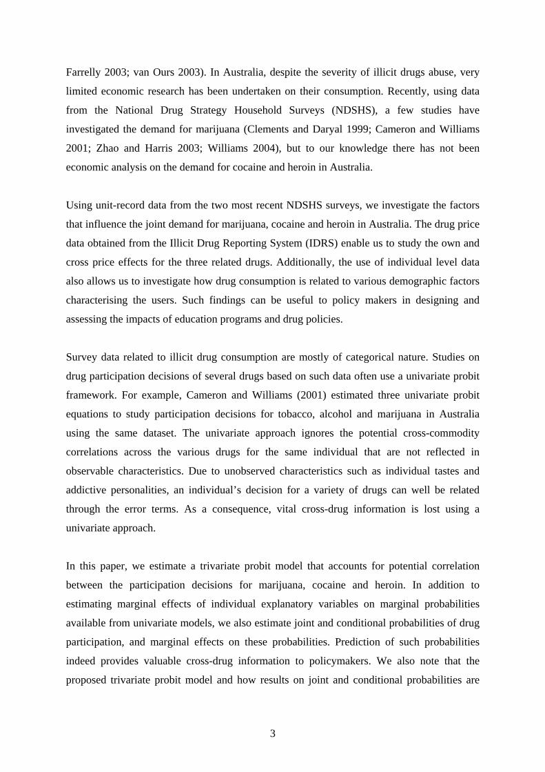
While the marginal probabilities are useful, the conditional probabilities of participation

given in Table 3 indicate how the consumptions of the three illicit drugs are related. For

instance, among those who consume heroin, 90.1% use marijuana and 63.5% use cocaine,

much higher than the unconditional probabilities of 14.6% and 1.4% respectively. As high as

86% of cocaine users consume marijuana and 23.3% of them use heroin. Among those who

consume cocaine and heroin jointly, 94.8% are marijuana users. Thus, we see that the chance

of an individual participating in a particular drug is much higher if he/she is known to be

taking other drug(s). These sample statistics indicate strong correlation across the three drugs.

A formal econometric model will allow the estimation of conditional correlations after

observable explanatory factors are controlled.

Table 3: Sample Participation Probabilitiesa

Marijuana Cocaine Heroin

P(. ) 14.55 1.35 0.50

P(.| )YM = 1 100.00 8.03 3.07

P(.| )YC = 1 86.23 100.00 23.28

P(.| )YH = 1 90.06 63.54 100.00

P(.| , )Y YC H= =1 1 94.78 100.00 100.00

P(.| , )Y YM H= =1 1 100.00 66.87 100.00

P(. | , )Y YM C= =1 1 100.00 100.00 25.59 a Probabilities are calculated from Table 2.

Price series for marijuana, cocaine and heroin for individual years and states/territories are

obtained mostly from the Illicit Drug Reporting System (IDRS, 2003). They correspond to

prices per ounce of marijuana and per gram of cocaine and heroin. The IDRS drug prices are

collected from interviewing injecting drug users and key informants who have regular

contacts with illicit drug users. In occasional cases where a price report is missing for a

particular state, we have constructed the price using information from the Australian Bureau

of Criminal Intelligence (ABCI, 2002). The ABCI (2002) is an alternative source for drug

6

prices, with information supplied by covert police units and police informants. We have

opted to use the price data from IDRS which are provided with unified measures and fewer

missing observations. Consumer Price Indexes by states for all groups come from the

Australian Bureau of Statistics (ABS 2003) and are used to deflate all three price series as

well as personal incomes of individuals.

In addition to information on drug use, the NDSHSs also contain details on personal

characteristics of respondents such as gender, marital status, educational attainment,

occupational status, household structure, income, etc. These are potential explanatory

variables in the econometric model to account for heterogeneity in participation decisions.

Details on definition of variables and sample statistics are outlined in the Appendix.

Table 4 highlights some cross statistics that provide information on how the participation in

marijuana, cocaine and heroin relate to the various demographic groups. These figures

represent proportions of individuals who consume the respective drugs in each population

group. It appears that males are more likely to consume all three drugs than females. Single

individuals have much higher chances of consuming all drugs than those who are married. In

terms of main activity, the highest proportions of marijuana or heroin use are recorded for the

unemployed individuals, followed by those whose main activity is studying. In fact, the

highest proportion of cocaine use is observed in the student group. In terms of educational

attainment, it appears that those with year-12 qualifications are more likely to use drugs than

those with higher qualifications or those with less than year-12 qualifications.

Also noted is that Aboriginals/Torres Strait Islanders (ATSI) have almost twice the chances

of using the drugs than non-aboriginals. Those who have pre-school children in the household

have lower chances of using these drugs than the rest. However, in terms of household

structure, single parents with dependent children have much higher chances to consume the

three drugs than the rest. Correlation with personal income is not straightforward from the

sample statistics. Marijuana use is highest among the low and middle income earners, while

heroin prevalence is highest in low income or higher-middle income earners. Cocaine

prevalence seems to fluctuate between one and two percent, with the highest percentages

observed among middle and very high income earners.

7

Table 4: Observed Participation Proportions by User Typea

Marijuana Cocaine Heroin

MALE 17.14 1.61 0.57 FEMALE 12.42 1.15 0.43 MARRIED 8.61 0.68 0.25 SINGLE 28.37 3.05 1.04 WORK 16.43 1.74 0.45 STUDY 24.93 2.05 0.68 UNEMPL 28.80 1.60 1.52 OTHERACT 5.87 0.40 0.39 DEGREE 13.35 1.76 0.33 DIPLOMA 14.49 1.38 0.36 YR12 19.14 1.79 0.75 LESSYR12 12.27 0.73 0.55 PRESCHOOL 12.98 1.27 0.32 NO-PRESCHOOL 14.75 1.36 0.52 ATSI 26.45 2.20 1.10 NON-ATSI 14.30 1.34 0.48 CAPITAL 15.57 1.70 0.57 NON-CAPITAL 12.09 0.54 0.33 SIN-PARENT 25.42 1.82 1.20 OTHERHHLD 13.72 1.32 0.44 INCOME: $0-$9,999 14.78 0.99 0.65 $10,000-$19,999 16.60 1.38 0.34 $20,000-$29,999 17.56 1.94 0.52 $30,000-$39,999 14.40 1.98 0.32 $40,000-$49,000 14.21 1.02 0.76 $50,000-$59,000 12.34 1.26 0.21 $60,000 or more 11.49 1.92 0.14

a Percentage of participation out of total for each demographic group.

3. The Multivariate Probit Model for Illicit Drug Participation

We assume that there is an underlying latent propensity variable Y (whereY ) that

is proportional to the unobserved level of demand for each of the three illicit drugs j

j∗

j∗ ⊂ −∞ ∞( , )

( , ,j )M C H= . The latent demand is determined by:

8

, (1) Y X j M C Hj j j j∗ = ′ + =β ε ( , , )

where represents a vector of observed personal characteristics and other economic

variables that affect the consumption of drug j,

X j

β j is a vector of unknown parameters, and

ε j is the error term. Equation (1) is mapped to an observable binary discrete variable Y

indicating whether or not an individual consumes a particular drug:

j

YYY

j M C Hjj

j

=>≤

RS|T|=

1 00 0

ifif

*

* ( , , ) . (2)

If we assume that ε j ( , ,j )M C H= are independently and identically distributed with a

standard normal distribution, equations (1) and (2) define three univariate probit (UVP)

models. The assumption of independent error terms in the UVP means that information about

an individual’s participation in one drug does not alter the prediction of the participation

probability of the same person for another drug.

A more general specification is to assume that the error terms in the three latent equations in

(1) jointly follow a multivariate normal distribution, that is, ( , , )' ~ ( , )ε ε εM C H MVN 0 Σ ,

where the variance-covariance matrix ∑ is given by

∑ =F

HGG

I

KJJ

11

1

ρ ρρρ ρ

MC MH

MC CH

MH CH

ρ , (3)

and where ρij is the correlation coefficient of ε i and ε j ( , , , ; )i j M C H i j= ≠ . Under this

assumption, equations (1) and (2) give a multivariate probit (MVP) model that jointly

represents the participation decisions for the three drugs. The MVP specification with

potentially non-zero off-diagonal elements in ∑ allows for correlations across the

disturbances of the three latent equations, which embody unobserved characteristics for the

same individuals. While the MVP model has the UVP as a special case, it now allows for the

knowledge on an individual’s participation in one drug to help predicting his/her probability

9

of participating in a related drug. Note that the assumption of unit variance for ε j ensures

that the β j parameters can be identified separately from the variance ofε j ( , ,j )M C H= .

The univariate marginal probability for participation in each drug is given:

P Y X Xj j j j( ) ( '= =1 1Φ β ) ( , , )j M C H= , (4)

where is the cumulative univariate distribution function for standard normal

distribution.

Φ1(.)

The bivariate joint probabilities are given by ( , , , ; )i j M C H i j= ≠ :

P Y Y X X X X

P Y Y X X X X

P Y Y X X X X

i i i i j j i

i i i i j j

i i i i j

j j

j j

j j

( , , ) ( , ; ),

( , , ) ( , ; )

( , , ) ( , ;

' '

' '

' '

= = =

= = = − −

= = = − −

1 1

1 0

0 0

2

2

2

Φ

Φ

Φ

β β ρ

β β ρ

β β ρ

.

j

ij

j ij

,

)

(5)

where Φ2 1 2 12( , ; )z z γ denotes the cumulative distribution function of standard bivariate

normal distribution with γ 12 as the correlation coefficient between the two univariate random

elements and . Z1 Z2

The multivariate joint probabilities are given by ( , , , , ; , ; )i j k M C H i j i k j k= ≠ ≠ ≠ :

P Y Y Y X X X X X X

P Y Y Y X X X X X X

P Y Y Y X X X X X X

P Y

i k i k i i j j k k ij ik jk

i k i k i i j j k k ij ik jk

i k i k i i j j k k ij ik jk

j j

j j

j j

( , , , , ) ( , , ; , , ),

( , , , , ) ( , , ; , , ),

( , , , , ) ( , , ; , , ),

(

' ' '

' ' '

' ' '

= = = =

= = = = − − −

= = = = − − − −

1 1 1

1 1 0

1 0 0

3

3

3

Φ

Φ

Φ

β β β ρ ρ ρ

β β β ρ ρ ρ

β β β ρ ρ ρ

i k i k i i j j k k ij ik jkY Y X X X X X Xj j= = = = − − −0 0 0 3, , , , ) ( , , ; , , ),' ' 'Φ β β β ρ ρ ρ etc.

(6)

10

where Φ3 1 2 3 12 13 23( , , ; , , )z z z γ γ γ denotes the cumulative distribution function of standard

trivariate normal distribution with γ st as the correlation coefficient between two of the three

univariate random elements and ( ,Zs Zt , , ; )s t s t= ≠1 2 3 .

Various conditional probabilities can also be similarly defined. Below are a few such

conditional probabilities:

P Y Y Y X X XX X X

X X

P Y Y Y X X XX X X

X X

P Y Y Y X X X

i j k i j ki i j j k k ij ik jk

j j k k jk

i j k i j ki i j j k k ij ik jk

j j k k jk

i j k i j k

( , ; , , )( , , ; , , )

( , ; ),

( , ; , , )( , , ; , ,

( , ; ),

( , ; , ,

= = = =

)

′ ′ ′

′ ′

= = = =′ − ′ − ′ − −

− ′ − ′

= = =

1 1 1

1 0 0

0 0 1

3

2

3

2

Φ

Φ

Φ

Φ

β β β ρ ρ ρ

β β ρ

β β β ρ ρ ρ

β β ρ

)( , , ; , , )

( ),

( ; , )( , ; )

( ),

=− ′ − ′ ′ − −

′

= = =′ ′

′

Φ

Φ

Φ

Φ

3

1

2

1

1 1

X X X

X

P Y Y X XX X

X

i i j j k k ij ik jk

k k

i j i ji i j j ij

j j

β β β ρ ρ ρ

β

β β ρ

β

etc.

(7)

Given an i.i.d. sample of N individuals and conditional on observed personal heterogeneity,

the MVP model can be estimated by maximising the following log-likelihood function:

log( ) ( , , ) log( ( , , , , )),L h i j k P Y i Y j Y k X X Xn Mkjin

N

C H Mn Cn Hn= = = =====∑∑∑∑

0

1

0

1

0

1

1

where

h i j kn Y i Y j Y k

i j knM C H( , , )

, , )( , , ).=

RST =10

0 1 if individual chooses ( = = = if otherwise.

or

4. Results

4.1 Results on Marginal Probabilities

11

The MVP model is estimated using the pooled sample of around 36,000 individuals from the

1998 and 2001 NDSHS surveys. We have used the same set of explanatory variables for all

three drug equations, so X X XM C H= X= ≡ . Table 5 gives estimates of the multivariate

probit model for marijuana, cocaine and heroin. Marginal effects (MEs) reported in this table

correspond to those of univariate marginal probabilities. For each continuous explanatory

variable the MEs relate to the absolute change in the unconditional probability of

participation for a particular drug in response to a unit change in the explanatory variable,

while for a dummy variable it represents the change in the probability when the dummy

variable changes from 0 to 1, all evaluated at the sample means of the other explanatory

variables2. Standard errors are reported in parentheses.

Table 5: Results of the MVP Modela

Marijuana Cocaine Heroin

Coefficient Marginal Effect Coefficient Marginal Effect Coefficient Marginal EffectCONSTANT -16.966 (1.088)** -2.862 (0.153)** -22.999 (2.771)** -0.248 (0.026)** -22.477 (5.314)** -0.109 (0.022)**

PRH 0.162 (0.045)** 0.027 (0.009)** -0.221 (0.112)** -0.002 (0.001)** 0.048 (0.177) 0.000 (0.000)

PRC 0.233 (0.051)** 0.039 (0.013)** 0.032 (0.158) 0.000 (0.002) 0.081 (0.170) 0.000 (0.001)

PRM -0.121 (0.079) -0.020 (0.013) 0.387 (0.197)** 0.004 (0.002)* 0.757 (0.510) 0.004 (0.002)*

INCOME 0.038 (0.016)** 0.006 (0.001)** 0.153 (0.039)** 0.002 (0.000)** -0.044 (0.060) 0.000 (0.000)

CAPITAL 0.020 (0.025) 0.003 (0.002)* 0.341 (0.064)** 0.004 (0.001)** 0.128 (0.093) 0.001 (0.000)

YR01 -0.065 (0.032)** -0.011 (0.006)* 0.126 (0.075)* 0.001 (0.001) -0.255 (0.163) -0.001 (0.001)*

AGE 9.563 (0.555)** 1.614 (0.045)** 11.546 (1.387)** 0.125 (0.010)** 9.857 (2.303)* 0.048 (0.007)**

AGESQ -1.550 (0.079)** -0.261 (0.006)** -1.809 (0.200)** -0.020 (0.002)** -1.499 (0.341)** -0.007 (0.001)**

MALE 0.279 (0.022)** 0.047 (0.002)** 0.113 (0.046)** 0.001 (0.000)** 0.222 (0.083)** 0.001 (0.000)**

MARRIED -0.410 (0.025)** -0.069 (0.004)** -0.457 (0.057)** -0.005 (0.001)** -0.418 (0.094)** -0.002 (0.001)**

WORK -0.047 (0.037) -0.008 (0.005)* 0.014 (0.094) 0.000 (0.001) -0.236 (0.118)** -0.001 (0.000)**

STUDY -0.051 (0.046) -0.009 (0.009) 0.134 (0.104) 0.001 (0.001) -0.268 (0.129)** -0.001 (0.000)**

UNEMP 0.290 (0.058)** 0.049 (0.004)** 0.058 (0.138) 0.001 (0.002) 0.036 (0.150) 0.000 (0.001)

PRESCHOOL -0.106 (0.031)** -0.018 (0.005)** -0.122 (0.073)* -0.001 (0.001)* 0.111 (0.111) 0.001 (0.000)

ATSI 0.208 (0.072)** 0.035 (0.018)* 0.108 (0.171) 0.001 (0.002) -0.101 (0.303) 0.000 (0.002)

DEGREE -0.080 (0.034)** -0.013 (0.005)** 0.020 (0.074) 0.000 (0.001) -0.403 (0.115)** -0.002 (0.000)**

DIPLOMA 0.033 (0.031) 0.006 (0.004) 0.051 (0.070) 0.001 (0.001) -0.287 (0.095)** -0.001 (0.000)**

YR12 0.008 (0.032) 0.001 (0.004) -0.001 (0.072) 0.000 (0.001) -0.235 (0.097)** -0.001 (0.000)**

SIN-PARENT 0.133 (0.038)** 0.023 (0.010)** -0.027 (0.082) 0.000 (0.001) 0.178 (0.096)* 0.001 (0.000)** ρMC 0.651 (0.023)** ρMH 0.590 (0.044)** ρCH 0.835 (0.026)**

2 Alternatively, we can compute the average MEs over all individuals. Harris et al. (2004) estimated MEs for a different discrete choice model using both approaches and found that the difference between them was trivial.

12

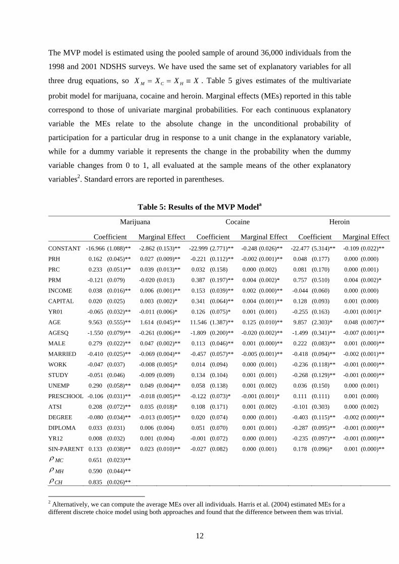
a. Standard errors are given in parentheses. * indicates significance at 10% level. **indicates significance at 5% level.

The last three rows of Table 5 show the estimated correlation coefficients

ρ ij i j M C H i j' ( , , , ; )s = ≠ . As expected, after accounting for impacts of observable

individual heterogeneity and economic factors, there still remains a strong positive

correlation among the participation decisions of the three drugs for the same individual. This

correlation is likely to be induced by unobservable personal characteristics such as taste and

addiction that have similar effects on individuals’ consumption of the three drugs. All three

correlation coefficients are statistically significant at the 1% level. This suggests that the null

hypothesis of three UVP models, or the hypothesis of independence across the error terms of

the three latent equations, can be rejected, and the MVP model is a better model for the

observed data. In particular, a correlation coefficient of 0.65 is estimated between the error

terms for marijuana and cocaine, 0.59 between those for marijuana and heroin, and the

highest correlation of 0.84 is observed between cocaine and heroin. It appears that being hard

drugs, cocaine and heroin are more strongly related in consumption.

Turning to the effects of observed explanatory factors, we start with the impacts of personal

characteristics. The knowledge of the vulnerable population segments for drugs can be useful

to policy makers in designing effective anti-drug programs. Prior studies have shown that

participation probabilities for recreational drugs are highest among young adults as compared

to teenagers and elderly people. To allow for this non-linear relationship, we have entered a

“squared” variable for age in the model. In all three equations, we obtain significant effects

for both the linear and quadratic age terms. To illustrate the combined effect of the two age-

related variables we estimate participation probabilities for a range of different age values as

plotted in Figure 1, holding all other explanatory variables fixed at mean values. In particular,

holding other factors at the same values, we find that the highest rate of participation for

marijuana is predicted among users who are in their early twenties. Cocaine is more popular

among individuals who are in their mid-twenties, while the highest participation in heroin

usage is observed among users in their late twenties. Overall, individuals in the age group 20-

30 years are mostly likely to be drug users.

Looking at the marginal effects of other demographic factors, other factors being constant,

we find that males are 4.7% more likely to use marijuana and 0.1% more likely to engage in

cocaine or heroin consumption than females. As compared to single individuals, married or

13

partnered individuals are 6.9%, 0.5% and 0.2% less likely to use marijuana, cocaine and

heroin respectively. With respect to individuals’ main occupation, relative to the group of

individuals who are pensioners or retired or who mainly perform home duties

(‘OTHERACT’=1), it appears that those who work have 0.8% and 0.1% less chances to

consume marijuana and heroin respectively, those who study are 0.1% less likely to consume

heroin, and those who are unemployed have 4.9% more chances of engaging in marijuana

consumption. Controlling for all other factors, it appears that main activity of individuals has

no significant partial effect on cocaine consumption.

Figure 1: Participation Probabilities by Age

0.00

0.05

0.10

0.15

0.20

0.25

0.30

0.35

10 20 30 40 50 60 70 80 90Age

Prob

abilit

y of

Mar

ijuan

a U

sage

0.000

0.005

0.010

0.015

0.020

0.025

0.030

Prob

abilit

y of

Coc

aine

& H

eroi

n U

sage

Marijuana

Cocaine

Heroin

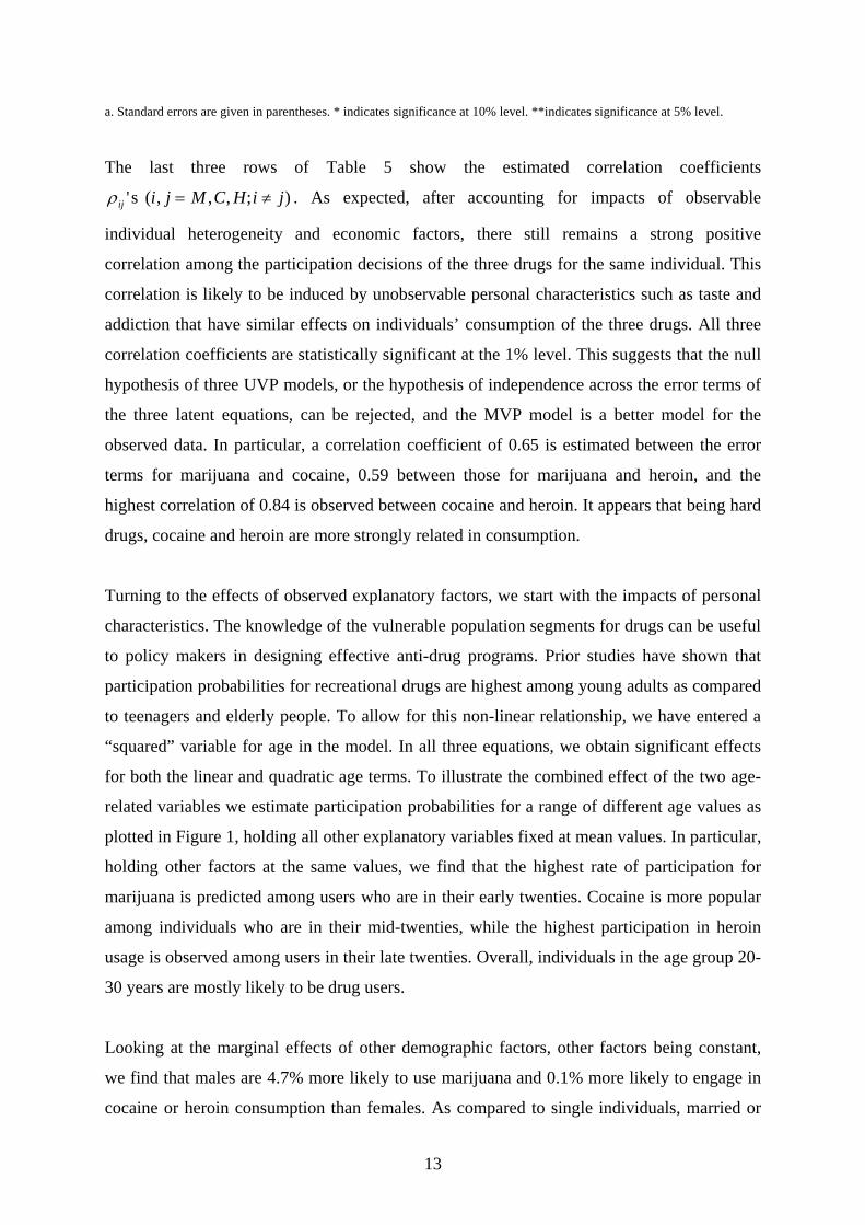
The presence of pre-school children in the household decreases the chances of consuming

marijuana and cocaine by 1.8% and 0.1% respectively. Aboriginals/Torres Strait Islanders

(ATSI) have 3.5% higher chances of using marijuana than non-aboriginals. Those living in

capital cities have 0.3% and 0.4% more chances in participating in marijuana and cocaine

consumption respectively. While there appears to be no correlation between education and

the use of cocaine, those who hold a degree have 1.3% less chances of using marijuana than

those with less than year-12 education. As for heroin, it appears that all other education

groups are significantly less likely to participate than the less than year-12 group. In

particular, degree holders are 0.2% less likely and those with a diploma or year-12 have 0.1%

less chances to use heroin than those in the lowest education band. People who did not finish

year-12 seem to be the most vulnerable group for heroin. Finally, being a single parent

14

increases the chances of using marijuana and heroin by 2.3% and 0.1% respectively. The

predicted probabilities for some of the demographic groups, holding other factors at mean

values, are illustrated in Figures 2-4.

In terms of personal income, we find that at the 5% significance level, it is positively related

to marijuana and cocaine participation when other factors are held constant. In particular, a

10% increase in income on average seems to increase the participation probabilities for

marijuana and cocaine by 0.06 and 0.02 percentage points respectively. For a total population

of 15 million aged 14 and above in Australia, these marginal effects translate into about 9,500

and 2,500 more marijuana and cocaine users respectively. However, we do not observe any

significant effect of income on heroin usage.

Finally, the drug price effects indicate that neither cocaine nor heroin participation is

responsive to their own prices, while there appears to be some evidence (with a p-value of

0.13) of own price response for marijuana. To the extent the price data are representative of

the true drug prices facing each individual, the cross price results provide some indication

about the economic relationships across the drugs. In particular, we find that marijuana

demand seems to respond to changes in the prices of harder drugs, such that a 10% increase

in the respective prices of cocaine and heroin increases the prevalence of marijuana use by

0.39 and 0.27 percentage points. However, there seems to be only weak evidence that an

increase in the price of marijuana will lead to an increased participation in cocaine and heroin

usage. Lastly, we find that an increase in the price of heroin decreases the participation

probability for cocaine. However, we recognise the lack of variation in our price data, given

that they vary by years and states, and deem individual level prices more appropriate.

Figure 2. Predicted Probabilities by Groups - Marijuana

15

0.00

0.02

0.04

0.06

0.08

0.10

0.12

0.14

0.16

0.18

GENDER MARITAL STATUS SINGLE PARENT MAIN ACTIVITY EDUCATION

Prob

abili

ty o

f Mar

ijuan

a C

onsu

mpt

ion

MALE

FEMALE

MARRIE

SINGLE

WORK

STUDY

UNEMPLOYED

OTHERACTIV

DEGREE

DIPLOMA

YEAR12QUAL

LESSYR12

SINGLEPARENT

OTHER

Figure 3. Predicted Probabilities by Groups - Cocaine

0.000

0.001

0.002

0.003

0.004

0.005

0.006

0.007

0.008

GENDER MARITAL STATUS CAPITAL PRESCHOOLCHILDREN

Prob

abili

ty o

f Coc

aine

Con

sum

ptio

n

MALE

FEMALE

MARRIE

SINGLE

PRESCH

OTHER

CAPIT

A

OTHER

Figure 4. Predicted Probabilities for Groups - Heroin

16

0.000

0.001

0.001

0.002

0.002

0.003

0.003

0.004

GENDER MARITAL STATUS SINGLE PARENT MAIN ACTIVITY EDUCATION

Pro

babi

lity

of H

eroi

n C

onsu

mpt

ion

MALE

FEMALE

MARRIE

SINGLE

SINGLEPARENT

OTHER

WORK

STUDY

UNEMPLOYED

OTHERACTI

V

DEGREE

DIPLOMA

YEAR12QUAL

LESSYR12

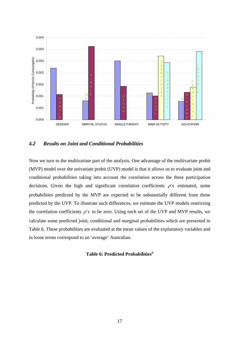
4.2 Results on Joint and Conditional Probabilities

Now we turn to the multivariate part of the analysis. One advantage of the multivariate probit

(MVP) model over the univariate probit (UVP) model is that it allows us to evaluate joint and

conditional probabilities taking into account the correlation across the three participation

decisions. Given the high and significant correlation coefficients ρ' s estimated, some

probabilities predicted by the MVP are expected to be substantially different from those

predicted by the UVP. To illustrate such differences, we estimate the UVP models restricting

the correlation coefficients ρ' s to be zero. Using each set of the UVP and MVP results, we

calculate some predicted joint, conditional and marginal probabilities which are presented in

Table 6. These probabilities are evaluated at the mean values of the explanatory variables and

in loose terms correspond to an ‘average’ Australian.

Table 6: Predicted Probabilitiesa

17

Marijuana Cocaine

MVP UVP MVP UVP

P( | )Y XM = 1 0.0948 0.0950 P( | )Y XC = 1 0.0036 0.0043 (0.0025) (0.0083) (0.0006) (0.0006) P( | )Y Y Y XM C H= = =1 0, 0, 0.0918 0.0950 P( | )Y Y Y XC M H= = =1 0, 0, 0.0007 0.0043 (0.0027) (0.0083) (0.0002) (0.0006) P( | , , )Y Y Y XM C H= = =1 1 1 0.8697 0.0950 P( | , , )Y Y Y XC M H= = =1 1 1 0.5692 0.0043 (0.0087) (0.0083) (0.0598) (0.0006) P( | , )Y Y XM C= =1 1 0.7943 0.0950 P( | , )Y Y XC M= =1 1 0.0302 0.0043 (0.0119) (0.0083) (0.0040) (0.0006) P( | , )Y Y XM H= =1 1 0.7785 0.0950 P( | , )Y Y XC H= =1 1 0.5095 0.0043 (0.0204) (0.0083) (0.0582) (0.0006)

Heroin Joint

MVP UVP MVP UVP

P( | )Y XH = 1 0.0015 0.0016 P( , , | )Y Y Y XM C H= = =1 1 1 0.0007 0.0000 (0.0005) (0.0003) (0.0001) (0.0000) P( | )Y Y Y XH M C= = =1 0, 0, 0.0003 0.0016 P( | )Y Y YM C H= = =0, 0, 0 X 0.9043 0.8997 (0.0001) (0.0003) (0.0029) (0.0083) P( | , , )Y Y Y XH M C= = =1 1 1 0.2308 0.0016 P( , | )Y Y Y XM C H= = =1 0, 0 0.0919 0.0945 (0.0537) (0.0003) (0.0028) (0.0083) P( | , )Y Y XH M= =1 1 0.0122 0.0016 P( , | )Y Y YM C H= = =0, 1 0 X 0.0007 0.0039 (0.0037) (0.0003) (0.0002) (0.0006) P( | , )Y Y XH C= =1 1 0.2108 0.0016 P( | )Y Y YM C H= = =0, 0, 1 X 0.0002 0.0014 (0.0469) (0.0003) (0.0001) (0.0003)

a Probabilities calculated at sample means of explanatory variables.

As shown in Table 6, with the UVP model, conditional and unconditional probabilities are

exactly the same given that participation decisions for the various drugs are independent. For

instance, even if an individual is known to be participating in both cocaine and heroin, his/her

probability for marijuana usage will be predicted by the UVP model as 9.5%, same as that if

the extra information is not available. However, taking into account the cross-equation

correlations, the individual’s marijuana participation probability is predicted by the MVP

model as high as 87%. Also, if an individual is known to be a heroin user, his/her

participation probability for cocaine is predicted to be 51% by the MVP model as against

0.4% by the UVP model. Using the UVP model, whether or not an individual is known to be

engaged in other drugs’ consumption, his/her probability of heroin consumption is predicted

as 0.2%. However, given that an individual consumes both cocaine and marijuana, his

chances of being a heroin user is higher at 23% using the MVP model. Similarly, joint

probabilities in the UVP model are obtained from multiplying the relevant marginal

probabilities, ignoring the positive links across uses of different drugs. Once the association

18

of the various choices are taken into account in the MVP, the predicted joint probabilities for

participating in all three drugs as well as for abstaining from all three drugs are higher than

those from the UVP.

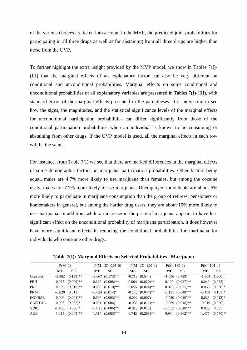
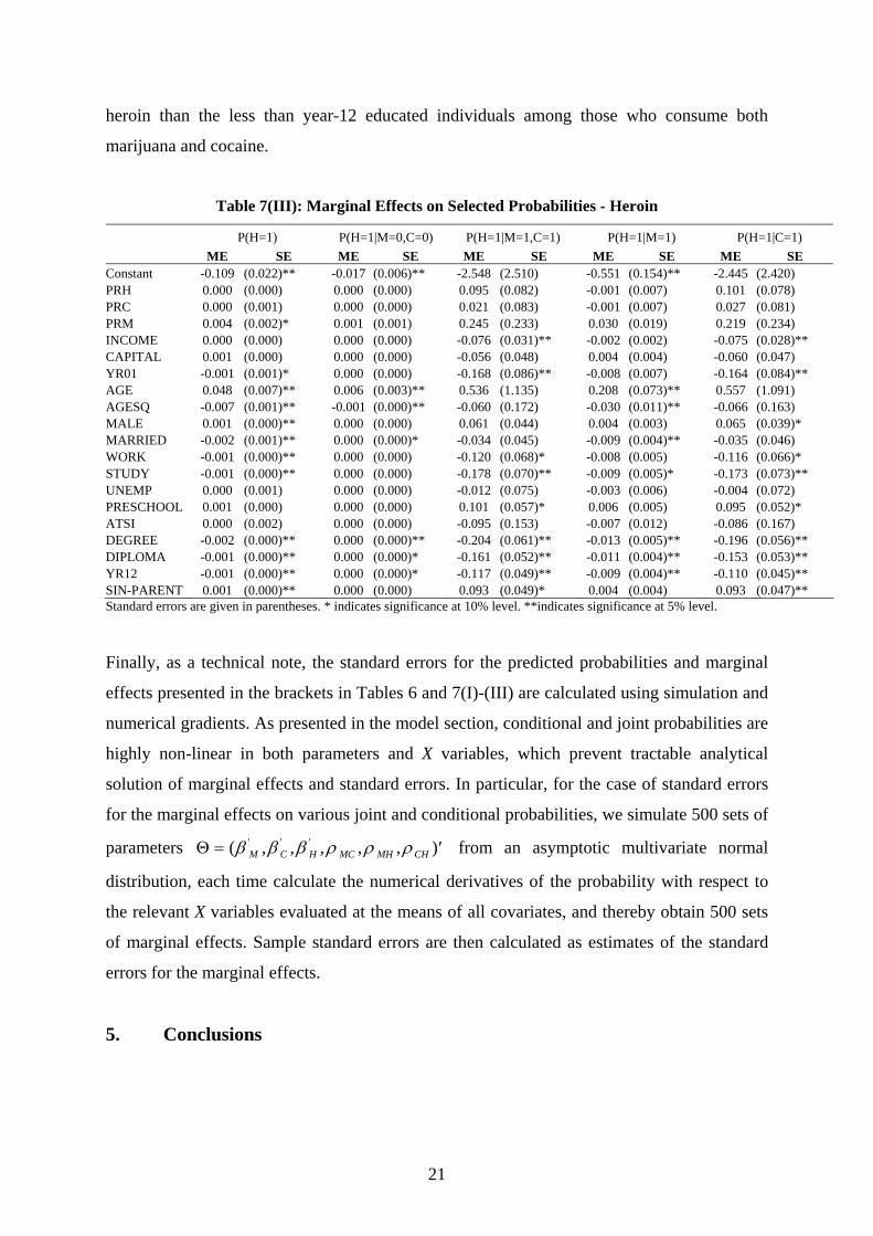
To further highlight the extra insight provided by the MVP model, we show in Tables 7(I)-

(III) that the marginal effects of an explanatory factor can also be very different on

conditional and unconditional probabilities. Marginal effects on some conditional and

unconditional probabilities of all explanatory variables are presented in Tables 7(I)-(III), with

standard errors of the marginal effects presented in the parentheses. It is interesting to see

how the signs, the magnitudes, and the statistical significance levels of the marginal effects

for unconditional participation probabilities can differ significantly from those of the

conditional participation probabilities when an individual is known to be consuming or

abstaining from other drugs. If the UVP model is used, all the marginal effects in each row

will be the same.

For instance, from Table 7(I) we see that there are marked differences in the marginal effects

of some demographic factors on marijuana participation probabilities. Other factors being

equal, males are 4.7% more likely to use marijuana than females, but among the cocaine

users, males are 7.7% more likely to use marijuana. Unemployed individuals are about 5%

more likely to participate in marijuana consumption than the group of retirees, pensioners or

homemakers in general, but among the harder drug users, they are about 10% more likely to

use marijuana. In addition, while an increase in the price of marijuana appears to have less

significant effect on the unconditional probability of marijuana participation, it does however

have more significant effects in reducing the conditional probabilities for marijuana for

individuals who consume other drugs.

Table 7(I): Marginal Effects on Selected Probabilities - Marijuana

P(M=1) P(M=1|C=0,H=0) P(M=1|C=1,H=1) P(M=1|C=1) P(M=1|H=1) ME SE ME SE ME SE ME SE ME SE Constant -2.862 (0.153)** -2.667 (0.173)** -0.713 (0.544) -1.096 (0.728) -1.604 (1.200) PRH 0.027 (0.009)** 0.028 (0.008)** 0.064 (0.020)** 0.109 (0.027)** 0.049 (0.038) PRC 0.039 (0.013)** 0.039 (0.010)** 0.055 (0.024)** 0.078 (0.035)** 0.068 (0.038)* PRM -0.020 (0.013) -0.024 (0.014)* -0.126 (0.047)** -0.131 (0.048)** -0.198 (0.105)* INCOME 0.006 (0.001)** 0.006 (0.003)** -0.002 (0.007) -0.020 (0.010)** 0.023 (0.013)* CAPITAL 0.003 (0.002)* 0.001 (0.004) -0.038 (0.011)** -0.069 (0.016)** -0.019 (0.020) YR01 -0.011 (0.006)* -0.011 (0.006)** -0.013 (0.017) -0.052 (0.018)** 0.028 (0.035) AGE 1.614 (0.045)** 1.517 (0.085)** 0.743 (0.268)** 0.934 (0.362)** 1.477 (0.570)**

19

AGESQ -0.261 (0.006)** -0.246 (0.012)** -0.134 (0.040)** -0.165 (0.053)** -0.259 (0.086)** MALE 0.047 (0.002)** 0.046 (0.004)** 0.049 (0.010)** 0.077 (0.012)** 0.056 (0.018)** MARRIED -0.069 (0.004)** -0.065 (0.004)** -0.036 (0.011)** -0.049 (0.014)** -0.064 (0.022)** WORK -0.008 (0.005)* -0.008 (0.006) 0.002 (0.015) -0.020 (0.022) 0.031 (0.026) STUDY -0.009 (0.009) -0.009 (0.008) -0.009 (0.018) -0.048 (0.025)* 0.036 (0.028) UNEMP 0.049 (0.004)** 0.048 (0.009)** 0.071 (0.024)** 0.094 (0.035)** 0.098 (0.033)** PRESCHOOL -0.018 (0.005)** -0.017 (0.005)** -0.024 (0.013)* -0.012 (0.017) -0.061 (0.024)** ATSI 0.035 (0.018)* 0.034 (0.013)** 0.053 (0.031)* 0.052 (0.042) 0.096 (0.064) DEGREE -0.013 (0.005)** -0.013 (0.006)** 0.004 (0.014) -0.034 (0.018)* 0.053 (0.026)** DIPLOMA 0.006 (0.004) 0.006 (0.005) 0.024 (0.013)* 0.001 (0.017) 0.070 (0.023)** YR12 0.001 (0.004) 0.002 (0.006) 0.019 (0.013) 0.003 (0.018) 0.051 (0.022)** SIN-PARENT 0.023 (0.010)** 0.022 (0.006)** 0.027 (0.014)* 0.055 (0.020)** 0.012 (0.022) Standard errors are given in parentheses. * indicates significance at 10% level. **indicates significance at 5% level.

Table 7(II): Marginal Effects on Selected Probabilities - Cocaine

P(C=1) P(C=1|M=0,H=0) P(C=1|M=1,H=1) P(C=1|M=1) P(C=1|H=1) ME SE ME SE ME SE ME SE ME SE Constant -0.248 (0.026)** -0.046 (0.010)** -3.448 (3.027) -1.209 (0.193)** -3.719 (3.135) PRP -0.002 (0.001)** -0.001 (0.000)** -0.189 (0.092)** -0.025 (0.009)** -0.174 (0.100)* PRC 0.000 (0.002) 0.000 (0.001) -0.038 (0.118) -0.007 (0.011) -0.021 (0.114) PRM 0.004 (0.002)* 0.001 (0.001) -0.089 (0.255) 0.037 (0.016)** -0.136 (0.275) INCOME 0.002 (0.000)** 0.000 (0.000)** 0.123 (0.033)** 0.011 (0.004)** 0.126 (0.038)** CAPITAL 0.004 (0.001)** 0.001 (0.000)** 0.170 (0.055)** 0.027 (0.006)** 0.162 (0.055)** YR01 0.001 (0.001) 0.001 (0.000)** 0.215 (0.082)** 0.013 (0.006)** 0.219 (0.090)** AGE 0.125 (0.010)** 0.022 (0.004)** 2.326 (1.381)* 0.565 (0.094)** 2.613 (1.401)* AGESQ -0.020 (0.002)** -0.003 (0.001)** -0.382 (0.206)* -0.087 (0.013)** -0.433 (0.207)** MALE 0.001 (0.000)** 0.000 (0.000) -0.054 (0.044) -0.002 (0.004) -0.040 (0.044) MARRIED -0.005 (0.001)** -0.001 (0.000)** -0.076 (0.055) -0.021 (0.005)** -0.089 (0.055)* WORK 0.000 (0.001) 0.000 (0.000) 0.127 (0.077)* 0.003 (0.008) 0.133 (0.078)* STUDY 0.001 (0.001) 0.001 (0.000) 0.225 (0.078)** 0.013 (0.008) 0.230 (0.085)** UNEMP 0.001 (0.002) 0.000 (0.000) -0.003 (0.095) -0.007 (0.012) 0.020 (0.096) PRESCHOOL -0.001 (0.001)* 0.000 (0.000) -0.127 (0.063)** -0.006 (0.006) -0.140 (0.064)** ATSI 0.001 (0.002) 0.000 (0.001) 0.105 (0.187) 0.001 (0.014) 0.126 (0.204) DEGREE 0.000 (0.001) 0.000 (0.000) 0.215 (0.062)** 0.005 (0.006) 0.225 (0.066)** DIPLOMA 0.001 (0.001) 0.000 (0.000) 0.170 (0.057)** 0.003 (0.005) 0.184 (0.058)** YR12 0.000 (0.001) 0.000 (0.000) 0.112 (0.055)** 0.000 (0.006) 0.122 (0.060)** SIN-PARENT 0.000 (0.001) 0.000 (0.000) -0.116 (0.058)** -0.008 (0.007) -0.111 (0.060)* Standard errors are given in parentheses. * indicates significance at 10% level. **indicates significance at 5% level.

From Table 7(II), we also see that those who are married or partnered have 0.5% less chances

of consuming cocaine than single individuals, but are 0.1% less likely to do so if they are

abstainers of other drugs and 7.6% less likely to do so if they use both of other two drugs.

Other factors controlled, individuals who study have as much chances to use cocaine as the

base group of retirees, pensioners and homemakers but are about 23% more likely to do so

given that they consume marijuana and heroin. In Table 7(III), we see that while educational

attainment seems to have only negligible effect on heroin consumption, holders of a degree,

diploma and year-12 qualifications are, respectively, 20%, 16% and 12% less likely to use

20

heroin than the less than year-12 educated individuals among those who consume both

marijuana and cocaine.

Table 7(III): Marginal Effects on Selected Probabilities - Heroin P(H=1) P(H=1|M=0,C=0) P(H=1|M=1,C=1) P(H=1|M=1) P(H=1|C=1) ME SE ME SE ME SE ME SE ME SE Constant -0.109 (0.022)** -0.017 (0.006)** -2.548 (2.510) -0.551 (0.154)** -2.445 (2.420) PRH 0.000 (0.000) 0.000 (0.000) 0.095 (0.082) -0.001 (0.007) 0.101 (0.078) PRC 0.000 (0.001) 0.000 (0.000) 0.021 (0.083) -0.001 (0.007) 0.027 (0.081) PRM 0.004 (0.002)* 0.001 (0.001) 0.245 (0.233) 0.030 (0.019) 0.219 (0.234) INCOME 0.000 (0.000) 0.000 (0.000) -0.076 (0.031)** -0.002 (0.002) -0.075 (0.028)** CAPITAL 0.001 (0.000) 0.000 (0.000) -0.056 (0.048) 0.004 (0.004) -0.060 (0.047) YR01 -0.001 (0.001)* 0.000 (0.000) -0.168 (0.086)** -0.008 (0.007) -0.164 (0.084)** AGE 0.048 (0.007)** 0.006 (0.003)** 0.536 (1.135) 0.208 (0.073)** 0.557 (1.091) AGESQ -0.007 (0.001)** -0.001 (0.000)** -0.060 (0.172) -0.030 (0.011)** -0.066 (0.163) MALE 0.001 (0.000)** 0.000 (0.000) 0.061 (0.044) 0.004 (0.003) 0.065 (0.039)* MARRIED -0.002 (0.001)** 0.000 (0.000)* -0.034 (0.045) -0.009 (0.004)** -0.035 (0.046) WORK -0.001 (0.000)** 0.000 (0.000) -0.120 (0.068)* -0.008 (0.005) -0.116 (0.066)* STUDY -0.001 (0.000)** 0.000 (0.000) -0.178 (0.070)** -0.009 (0.005)* -0.173 (0.073)** UNEMP 0.000 (0.001) 0.000 (0.000) -0.012 (0.075) -0.003 (0.006) -0.004 (0.072) PRESCHOOL 0.001 (0.000) 0.000 (0.000) 0.101 (0.057)* 0.006 (0.005) 0.095 (0.052)* ATSI 0.000 (0.002) 0.000 (0.000) -0.095 (0.153) -0.007 (0.012) -0.086 (0.167) DEGREE -0.002 (0.000)** 0.000 (0.000)** -0.204 (0.061)** -0.013 (0.005)** -0.196 (0.056)** DIPLOMA -0.001 (0.000)** 0.000 (0.000)* -0.161 (0.052)** -0.011 (0.004)** -0.153 (0.053)** YR12 -0.001 (0.000)** 0.000 (0.000)* -0.117 (0.049)** -0.009 (0.004)** -0.110 (0.045)** SIN-PARENT 0.001 (0.000)** 0.000 (0.000) 0.093 (0.049)* 0.004 (0.004) 0.093 (0.047)** Standard errors are given in parentheses. * indicates significance at 10% level. **indicates significance at 5% level.

Finally, as a technical note, the standard errors for the predicted probabilities and marginal

effects presented in the brackets in Tables 6 and 7(I)-(III) are calculated using simulation and

numerical gradients. As presented in the model section, conditional and joint probabilities are

highly non-linear in both parameters and X variables, which prevent tractable analytical

solution of marginal effects and standard errors. In particular, for the case of standard errors

for the marginal effects on various joint and conditional probabilities, we simulate 500 sets of

parameters from an asymptotic multivariate normal

distribution, each time calculate the numerical derivatives of the probability with respect to

the relevant X variables evaluated at the means of all covariates, and thereby obtain 500 sets

of marginal effects. Sample standard errors are then calculated as estimates of the standard

errors for the marginal effects.

Θ = ′( , , , , , )' ' 'β β β ρ ρ ρM C H MC MH CH

5. Conclusions

21

We investigate factors that influence the consumption of marijuana, cocaine and heroin in

Australia using unit-record data from national representative surveys involving more than

36,000 individuals. Recognising the potential association between the demands for the three

closely related drugs due to unobserved personal characteristics such as taste and addictive

personality, we estimate a multivariate probit (MVP) model where the three participation

equations are jointly estimated as a system with correlated error terms. The estimated

correlation coefficients between the three drugs are found to be very high and statistically

significant. The highest correlation is found between the two harder drugs, cocaine and

heroin, which are more similar in nature as compared to marijuana.

To highlight the advantages of the MVP model over the typically used univariate probit

(UVP) model where correlations across drug equations are restricted to zero, we compare the

predicted marginal, conditional and joint probabilities using the two approaches. The results

show that the MVP model provides better predictions than the UVP model in terms of

conditional and joint probabilities. The additional knowledge of an individual’s participation

(or abstention) in other drugs can significantly alter his or her probability of consuming a

particular drug.

We also estimate the marginal effects of individual explanatory factors on marginal, joint and

conditional probabilities. They shed important insights on the effects of prices and other

demographic factors on participation probabilities when the user is known to be consuming

or abstaining from related drugs. The results indicate that the marginal effect of a particular

independent variable and their statistical significance can be very different for conditional

and unconditional participation probabilities. These extra insights on cross commodity

relationships provided by the MVP model are important to policy makers.

The study provides valuable empirical information on the consumer behaviour of illicit drugs.

While there are a range of studies on legal recreational drugs, illegal drug studies are much

fewer due to data scarcity. We investigate the effects of price, income and other demographic

factors on the demand for all three drugs. While acknowledging potential lack of variation in

the drug price data used, we find no significant own price responsiveness for cocaine and

heroin but some weak evidence of own price response for marijuana. Interestingly, the

negative own-price effect on marijuana participation is much larger and statistically

significant among users of other drugs. We also find some significant cross-price effects on

22

the demand for the three drugs. There is also some evidence of a positive income effect on

the use of marijuana and cocaine. Additionally, participation in the consumption of the three

drugs is shown to be related to social and demographic factors. Marijuana is most popular

among young adults in their early twenties and, other factors being equal, is more likely to be

consumed by individuals who are male, single, unemployed, aboriginals and single parents.

Cocaine is more associated with individuals in their mid twenties, male, single and who

reside in capital cities. The highest participation in heroin usage is observed among

individuals in their late twenties, less educated, male, and single, while lower participation

probability is found among individuals who work or study, other factors equal. The empirical

application indicates that important cross-drug information will be lost using a univariate

approach.

References

ABCI (2002). "Australian Illicit Drug Report", Australian Bureau of Criminal Intelligence. Commonwealth of Australia: Canberra. ABS (2003). Consumer Price Index 14th Series: By Region, All Groups, Cat. No. 640101b. Australian Bureau of Statistics. Becker, G. S. and K. M. Murphy (1988). "A Theory of Rational Addiction." Journal of Political Economy 96(4): 675-700. Cameron, L. and J. Williams (2001). "Cannabis, Alcohol and Cigarettes: Substitutes or Complements." The Economic Record 77(236): 19-34. Chaloupka, F. J., M. Grossman and J. A. Tauras (1998). The Demand for Cocaine and Marijuana by Youth. National Bureau of Economic Research. Working Paper 6411. Chaloupka, F. J. and A. Laixuthai (1997). "Do Youths Substitute Alcohol and Marijuana? Some Econometric Evidence." Eastern Economic Journal 23(3): 253. Clements, K. W. and M. Daryal (1999). The Economics of Marijuana Consumption. University of Western Australia, unpublished paper. Collins, D. J. and H. M. Lapsley (2002). Counting the Cost: Estimates of the Social Costs of Drug Abuse in Australia in 1998-99. Commonwealth Department of Human Services and Health: Canberra. Desimone, J. and M. C. Farrelly (2003). Price and Enforcement Effects on Cocaine and Marijuana Demand. Department of Economics, East Carolina University. Working Paper 0101.

23

DiNardo, J. (1993). "Law Enforcement, the Price of Cocaine and Cocaine Use." Mathematical and Computer Modeling 97(2). DiNardo, J. and T. Lemieux (2001). "Alcohol, Marijuana, and American Youth: The Unintended Consequences of Government Regulation." Journal of Health Economics 20(6): 991-1010. Farrelly, M. C., J. W. Bray, G. A. Zarkin and B. W. Wendling (2001). "The Joint Demand for Cigarettes and Marijuana: Evidence from the National Household Surveys on Drug Abuse." Journal of Health Economics 20(1): 51-68. Grossman, M. and F. J. Chaloupka (1998). "The Demand for Cocaine by Young Adults: A Rational Addiction Approach." Journal of Health Economics 17: 427–474. Harris, M., P. Ramful, and X. Zhao (2004), “Alcohol Consumption in Australia: An Application of the OGEV Model to Micro-Unit Data.”, Journal of Health Economics, forthcoming. IDRS (2003). "Australian Drug Trends", Illicit Drug Reporting System. National Drug and Alcohol Research Centre. Mathers, C., T. Vos and C. Stevenson (1999). The Burden of Disease and Injury in Australia. Australian Institute of Health and Welfare: Canberra. Model, K. E. (1993). "The Effect of Marijuana Decriminalisation on Hospital Emergency Room Drug Episodes: 1975-1978." Journal of the American Statistical Association 88(423): 737-747. NDSHS (2001). Computer Files, National Drug Strategy Household Surveys, 1998 and 2001, Social Science Data Archives, Australian National University, Canberra. Pacula, R. L. (1998a). Adolescent Alcohol and Marijuana Consumption: Is There Really a Gateway Effect? National Bureau of Economic Research. Working paper 6348. --- (1998b). "Does Increasing the Beer Tax Reduce Marijuana Consumption?" Journal of Health Economics 17(5): 557-585. Petry, N. M. (2001). "A Behavioral Economic Analysis of Polydrug Abuse in Alcoholics: Asymmetrical Substitution of Alcohol and Cocaine." Drug and Alcohol Dependence 62: 31-39. Saffer, H. and F. J. Chaloupka (1995). The Demand for Illicit Drugs, National Bureau of Economic Research. Working Paper 5238. --- (1998). Demographic Differentials in the Demand for Alcohol and Illicit Drugs. National Bureau of Economic Research. Working Paper 6432. --- (1999). "The Demand for Illicit Drugs." Economic Inquiry 37(3): 401-411.

24

Thies, C. F. and C. A. Register (1993). "Decriminalization of Marijuana and the Demand for Alcohol, Marijuana and Cocaine." Social Science Journal 30(4): 385-400. UNODC (2003). Global Illicit Drug Trends, 2003. United Nations Office on Drugs and Crime. Vienna, Austria, United Nations. van Ours, J. C. (2003). "Is Cannabis a Stepping-Stone for Cocaine?" Journal of Health Economics 22: 539–554. Weatherburn, D., C. Jones, K. Freeman and T. Makkai (2001). The Australian Heroin Drought and Its Implications for Drug Policy. Crime and Justice Bulletin. Number 59. Williams, J. (2004). "The Effects of Price and Policy on Marijuana Use: What Can Be Learned from the Australian Experience?" Health Economics 13: 123-137. Zhao, X. and M. Harris (2003). Demand for Marijuana, Alcohol and Tobacco: Participation, Levels of Consumption, and Cross-Equation Correlations. Paper presented at the Australasian Meeting of the Econometrics Society, July, Sydney.

25

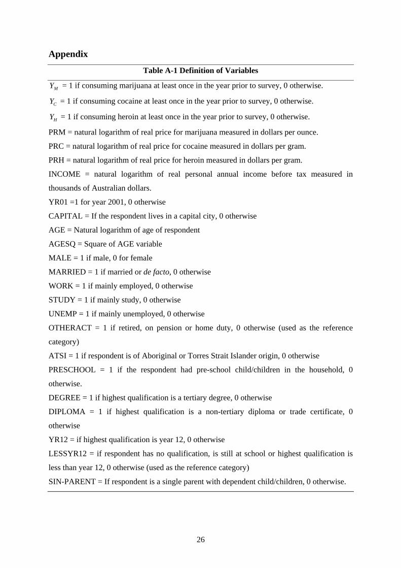
Appendix

Table A-1 Definition of Variables

YM = 1 if consuming marijuana at least once in the year prior to survey, 0 otherwise.

YC = 1 if consuming cocaine at least once in the year prior to survey, 0 otherwise.

YH = 1 if consuming heroin at least once in the year prior to survey, 0 otherwise.

PRM = natural logarithm of real price for marijuana measured in dollars per ounce.

PRC = natural logarithm of real price for cocaine measured in dollars per gram.

PRH = natural logarithm of real price for heroin measured in dollars per gram.

INCOME = natural logarithm of real personal annual income before tax measured in

thousands of Australian dollars.

YR01 =1 for year 2001, 0 otherwise

CAPITAL = If the respondent lives in a capital city, 0 otherwise

AGE = Natural logarithm of age of respondent

AGESQ = Square of AGE variable

MALE = 1 if male, 0 for female

MARRIED = 1 if married or de facto, 0 otherwise

WORK = 1 if mainly employed, 0 otherwise

STUDY = 1 if mainly study, 0 otherwise

UNEMP = 1 if mainly unemployed, 0 otherwise

OTHERACT = 1 if retired, on pension or home duty, 0 otherwise (used as the reference

category)

ATSI = 1 if respondent is of Aboriginal or Torres Strait Islander origin, 0 otherwise

PRESCHOOL = 1 if the respondent had pre-school child/children in the household, 0

otherwise.

DEGREE = 1 if highest qualification is a tertiary degree, 0 otherwise

DIPLOMA = 1 if highest qualification is a non-tertiary diploma or trade certificate, 0

otherwise

YR12 = if highest qualification is year 12, 0 otherwise

LESSYR12 = if respondent has no qualification, is still at school or highest qualification is

less than year 12, 0 otherwise (used as the reference category)

SIN-PARENT = If respondent is a single parent with dependent child/children, 0 otherwise.

26

Table A-2 Summary Statistics

Mean Std. Dev. Minimum Maximum Cases

Dependent Variables YM 0.145 0.352 0 1 36579 YC 0.014 0.116 0 1 36535 YH 0.005 0.070 0 1 36539 Explanatory Variables PRH 5.750 0.263 5.439 6.348 37081 PRC 5.169 0.238 4.818 5.824 37081 PRM 5.408 0.178 4.996 5.662 37081 INCOME 9.661 0.976 6.654 11.42 29141 CAPITAL 0.699 0.459 0 1 37084 YR01 0.721 0.448 0 1 37084 AGE 3.633 0.455 2.639 4.585 37080 AGESQ 13.41 3.252 6.965 21.02 37080 MALE 0.445 0.497 0 1 37084 MARRIED 0.565 0.496 0 1 36864 WORK 0.527 0.499 0 1 36230 STUDY 0.115 0.319 0 1 36230 UNEMP 0.037 0.188 0 1 36230 PRESCHOOL 0.138 0.345 0 1 36365 ATSI 0.018 0.132 0 1 36750 DEGREE 0.208 0.406 0 1 36390 DIPLOMA 0.276 0.447 0 1 36390 YR12 0.214 0.410 0 1 36006 SIN-PARENT 0.067 0.250 0 1 36293

27