86
644031-4 Demand forecast for Annual Security Assessment (from 2010) Prepared by Electricity Commission 26 October 2010
| Date post: | 24-Jun-2018 |
| Category: |
Documents |
| Upload: | vuongthuan |
| View: | 220 times |
| Download: | 0 times |
644031-4
Demand forecast for Annual Security Assessment (from 2010)
Prepared by Electricity Commission
26 October 2010


Demand forecast for Annual Security Assessment (from 2010)
644031-4 C
Executive summary
This document presents demand forecasts prepared for use in the 2010 Annual Security
Assessment (ASA).
Transpower must prepare and publish the 2010 ASA. As part of the transition of Security of
Supply monitoring and forecasting responsibilities, it has been agreed that the Commission
will provide a demand forecast for use in this assessment. Transpower will be responsible for
preparing forecasts for future assessments.
The report includes five-year forecasts of total annual energy demand (GWh), annual peak
demand (MW), and (new this year) the mean of the 200 highest half-hourly peaks.
Forecasts are provided for New Zealand as a whole, the North and South Islands, and the
four half-islands (Upper North, Lower North, Upper South, Lower South).
The forecasting methodology is essentially the same as that used in the 2007 and 2008
demand forecasts. It is based on:
stakeholder expert knowledge about specific existing and new loads; and
statistical extrapolation of other demand.
For 2011, the national energy forecasts are 40,466 GWh (expected, P50) and 41,798 GWh
(prudent, P95). These forecasts represent annual growth of 1.6% or 2.4% since 2007, in
which the energy demand was 38,034 GWh.
The expected rate of energy growth from 2011 to 2015 is 2.1%.
For 2011, the national half-hourly peak forecasts are 6,676 MW (expected, P50) and 6,931
MW (prudent, P95). These forecasts represent annual growth of 1.0% (expected) or 2.0%
(prudent) since 2007, in which the half-hourly peak was 6,405 MW.
The expected rate of peak growth from 2011 to 2015 is 2.0%.
Energy growth is predicted to be very similar across the two islands. Peak growth is
expected to be higher in the North Island (2.2%) than the South Island (1.7%).
The report discusses some unusual features of recent demand:
both peak and energy demand were low in 2009 and 2010, even allowing for reduced
demand at the Tiwai smelter; and
organic energy demand growth in the North Island has been low since 2006.
A low growth ("hockey stick") sensitivity scenario is included.

Demand forecast for Annual Security Assessment (from 2010)
D 644031-4
Glossary of abbreviations and terms
5% POE Forecast with 5% probability of exceedence, i.e. there is intended to
be a 5% chance that actual demand will be higher than forecast in
any given year. Also referred to as 'prudent forecast' and P95
50% POE Forecast with 50% probability of exceedence. Also referred to as
'expected forecast' and P50
Embedded
generator
Generator connected to a distribution network (as opposed to: grid-
connected generator)
Energy Used here in the sense of total electrical energy, denominated in
GWh. Energy forecast is used in the calculation of Winter Energy
Margin
Expected forecast See '50% POE'
Forecast Prediction of the future (c.f. 'projection', which is used in this
document to indicate a single possible sequence of future values -
many projections are combined to produce a single forecast)
Generation
component of
demand
Reduction in total demand (energy or peak) stemming from the
netted-off generators listed in Table 1 - always expressed as a
negative number (see also: industrial component of demand, residual
component of demand)
GPA Grid Planning Assumptions, as published in the Statement of
Opportunities
Grid-connected
generator
Generator connected directly to the national grid (as opposed to:
embedded generator)
GXP Grid Exit Point
Half-hourly peak Maximum half-hourly demand in a given time period, where half-
hourly demand is defined as the mean electricity demand in each
trading period and denominated in MW. C.f. instantaneous peak
Half-island One of the Upper North Island, Lower North Island, Upper South
Island and Lower South Island regions (see Section 1.5)
Industrial
component of
demand
Portion of total demand (energy or peak) stemming from the direct-
connect customers listed in Table 2 (see also: generation component
of demand, residual component of demand)
Instantaneous
peak
Maximum demand in a given period, where demand is measured at a
high frequency (e.g. every 10 seconds) and denominated in MW. C.f.
half-hourly peak
LNI, LSI Lower North Island and Lower South Island (see Section 1.5)

Demand forecast for Annual Security Assessment (from 2010)
644031-4 E
Netted-off
generation
Generation whose total output has been subtracted from the demand
forecast. Should not be modelled on the supply side (this would be
double counting).
NIPS North Island Public Supply (i.e. total electricity supplied by
generators)
P50, P95 See '50% POE' and ‘5% POE’
Projection In this document, used interchangeably with 'trajectory' to indicate a
single possible sequence of future values - a 'forecast' is calculated
as a summary of a set of projections
Prudent forecast See '5% POE'
RENA Reserve Energy Needs Assessment – older name for Annual Security
Assessment
Residual
component of
demand
Portion of total demand (energy or peak) that is left over after
'generation component' and 'industrial component' have been
subtracted
Short-term
variation factor
Factor applied to half-hourly peak demand forecasts to produce
instantaneous peak forecasts, reflecting the influence of within-half-
hour variation in demand
SIPS South Island Public Supply (i.e. total electricity supplied by
generators)
SOO Statement of Opportunities (contains Grid Planning Assumptions)
SSF Transpower's System Security Forecast
Temperature
correction factor
Factor measuring the effect of temperature on the residual
component of peak (or top200) demand. A high factor (substantially
over 1) means that cold winter temperatures led to high demand
Temperature-
corrected residual
demand
Residual component of peak (or top200) demand divided by the
temperature correction factor. Indicates the estimated value that
residual peak demand would have taken in a given year if
temperatures had been average
Top200 Mean of the highest 200 half-hourly peaks in a given year.
Denominated in MW. Used in the calculation of Winter Capacity
Margin
Trajectory Used interchangeably with 'projection'
UNI, USI Upper North Island, Upper South Island (see Section 1.5)
Winter Capacity
Margin, Winter
Energy Margin
Metrics used in the Annual Security Assessment

Demand forecast for Annual Security Assessment (from 2010)
F 644031-4
Demand forecast for Annual Security Assessment (from 2010)
644031-4 G
Contents
Executive summary C
Glossary of abbreviations and terms D
1. Introduction 1
1.1 Background 1
1.2 Scope of the forecast 2
1.3 Reactive demand growth - out of scope 3
1.4 Treatment of netted-off generation 4
1.5 Region definitions 7
2. Methodology 8
2.1 Overview 8
2.2 Data preparation – historical demand 11
2.3 Collection of information from stakeholders 12
2.4 Temperature vs peak demand modelling 13
2.5 Statistical analysis of residual demand 15
2.6 Assembling the forecasts 16
2.7 Instantaneous peak forecasts 18
3. Results 19
3.1 Historical demand data 19
3.2 Demand questionnaire findings 25
3.3 Temperature vs peak demand – results 27
3.4 Forecasts 32
3.5 Instantaneous peak forecasts 40
3.6 Changes since 2008 41
3.7 Caveats 44
4. Validation 45
4.1 Introduction 45
4.2 Validation of the predictions for 2009 and 2010 46
5. Comparisons with other published forecasts 51

Demand forecast for Annual Security Assessment (from 2010)
H 644031-4
5.1 Introduction 51
5.2 The 2010 GPA forecasts 51
6. Low growth ('hockey stick') sensitivity 56
6.1 Rationale 56
6.2 Assumptions 56
6.3 Results 56
Appendix 1 Gnash script used to produce the half-hourly demand
dataset 63
Appendix 2 Demand and embedded generation survey 66
Appendix 3 Historical demand data 68
Tables
Table 1 Netted-off generators 5
Table 2 Existing direct-connect customers in the industrial component 10
Table 3 Existing netted-off generators in the generation component 10
Table 4 Comparison of recent energy demand growth rates (excluding industrial and embedded generation components) 24
Table 5 Forecasts 32
Table 6 Short-term variation factors, as used to produce instantaneous peak forecasts 40
Table 7 Instantaneous peak forecasts 41
Table 8: Comparison between expected energy demand forecasts 42
Table 9: Comparison between prudent energy demand forecasts 42
Table 10: Comparison between expected halfhourly peak demand forecasts 42
Table 11: Comparison between prudent halfhourly peak demand forecasts 42
Table 12 Predicted 2009 half-hourly peaks vs actual values 46
Table 13 Predicted 2010 half-hourly peaks vs actual values 48
Table 14 Predicted 2009 energy vs actual values 49
Table 15 Energy forecasts - 'hockey stick' sensitivity 57
Table 16 Peak forecasts - 'hockey stick' sensitivity 59
Table 17 Historical energy demand data 68
Table 18 Historical half-hourly peak demand data 71
Table 19 Historical top200 demand data 74

Demand forecast for Annual Security Assessment (from 2010)
644031-4 I
Figures
Figure 1: A sample of 20 projections of the residual demand component 16
Figure 2: A sample of 20 projections of half-hourly peak demand 17
Figure 3: Historical demand data used in the forecast 20
Figure 4: Residual component of North Island energy demand 22
Figure 5: Residual component of North Island peak demand 23
Figure 6: Residual component of South Island energy demand 23
Figure 7: Residual demand component averaged over top 200 peaks - actual vs temperature-corrected 28
Figure 8: Residual demand component at half-hourly peak - actual vs temperature-corrected 29
Figure 9: Forecasts 35
Figure 10: Comparison between expected forecasts 43
Figure 11: Comparison with GPA energy forecasts (relative to 2007) 53
Figure 12 Comparison with GPA half-hourly peak forecasts (relative to 2007) 54
Figure 13 Energy forecasts - 'hockey stick' sensitivity 58
Figure 14 Peak forecasts - 'hockey stick' sensitivity 60


Demand forecast for Annual Security Assessment (from 2010)
644031-4 1
1. Introduction
1.1 Background
1.1.1 This document presents the energy and peak demand forecasts prepared for use
in the 2010 Annual Security Assessment (ASA).
1.1.2 The Commission has undertaken previous Annual Security Assessments (also
referred to as Reserve Energy Needs Assessments, RENA) to assess security of
supply and determine whether there is a need for additional reserve energy.
1.1.3 In 2007, a demand forecasting methodology was developed for use in the Annual
Security Assessment process and published for consultation.1 The new
methodology was implemented to prepare demand forecasts2 that were used in
the 2007 RENA.3
1.1.4 In 2008, the demand forecast was updated4 and used in the 2008 ASA.5
1.1.5 No new demand forecast was prepared for use in the 2009 ASA6, because it was
considered that there was not enough new data to justify the forecasting
exercise. (Data from winter 2008 were considered to be compromised by the dry
winter and public conservation campaign, and data from early-mid 2009 were
suspected to be affected by a short-term 'blip' caused by economic conditions.)
Instead, the assessment used the previous year’s demand forecast, with
modifications based on information collected through a confidential survey.
1.1.6 Transpower must prepare and publish the 2010 ASA, under its Security of Supply
Forecasting and Information Policy (SOSFIP).7 As part of the transition of
Security of Supply monitoring and forecasting responsibilities, it has been agreed
that the Commission will provide a demand forecast for use in this assessment.
1.1.7 Transpower will be responsible for preparing forecasts for future assessments.
1 http://www.ea.govt.nz/our-work/consultations/security-of-supply/demand-forecasting-methodology/
2 http://www.ea.govt.nz/document/11863/download/industry/ec-archive/security-of-supply/asa/archives/
3 http://www.ea.govt.nz/our-work/consultations/security-of-supply/asa-and-reserve-energy-needs-07/
4 http://www.ea.govt.nz/document/11864/download/industry/ec-archive/security-of-supply/asa/
5 http://www.ea.govt.nz/document/2397/download/industry/ec-archive/security-of-supply/asa/
6 http://www.ea.govt.nz/document/4550/download/industry/ec-archive/security-of-supply/asa/
7 http://www.systemoperator.co.nz/sos-policy

Demand forecast for Annual Security Assessment (from 2010)
2 644031-4
1.2 Scope of the forecast
1.2.1 The scope of this work is to produce forecasts of:
(a) energy – total annual energy demand (GWh);
(b) peak – annual half-hourly peak and instantaneous peak (both in MW); and
(c) top200 – the mean of the 200 highest half-hourly peaks in each year (MW).
1.2.2 The energy forecasts are used in the calculation of Winter Energy Margins, and
the top200 forecasts in the calculation of the Winter Capacity Margin.8
1.2.3 The peak forecasts are not strictly required for the Annual Security Assessment,
and are provided for information only.
1.2.4 It has been suggested that an MVA forecast should be included. No such
forecast has been included at this stage, though reactive power issues are
acknowledged as being important (Section 1.3).
1.2.5 Forecasts are presented at national, island and half-island9 levels. Note that peak
demand forecasts refer to national demand at national peak, island demand
at island peak, and half-island demand at half-island peak (rather than, say, half-
island demand at national peak time).
1.2.6 The forecast horizon covers five calendar years (not March years), from 2011 to
2015.
1.2.7 Both expected forecasts and more conservative 'prudent' forecasts have been
prepared.
1.2.8 All forecasts represent demand 'at grid exit point (GXP) level', i.e. inclusive of
distribution losses but exclusive of transmission losses. The output of some
(mostly embedded) generators has been netted off – see Section 1.4.
1.2.9 The aim of this work is to forecast demand in the absence of unusual demand
response. Demand-side response during periods of actual or potential scarcity
should be modelled outside the forecast.
8 http://www.ea.govt.nz/act-code-regs/code-regs/the-code/part-7/
9 I.e. Upper North Island, Lower North Island, Upper South Island and Lower South Island, as defined in Section
1.5.

Demand forecast for Annual Security Assessment (from 2010)
644031-4 3
1.3 Reactive demand growth - out of scope
1.3.1 There is a substantial requirement for reactive power investment in the Upper
North Island and Upper South Island.
1.3.2 In theory, these reactive power needs could be considered in the Annual Security
Assessment - in which case, a forecast of reactive demand would be required.
1.3.3 At this stage, however, it is not felt that it would be useful to do so - these issues
are better canvassed in other contexts. The Commission's recent consultation
paper on Stage 2 of the Transmission Pricing Review discusses the facilitation of
static reactive investment.10
1.3.4 For basic information on reactive growth in the last few years, see the following
IAG presentation: http://www.ea.govt.nz/document/3296/download/our-
work/advisory-working-groups/iag/iag-meeting-11-february-2010/.
1.3.5 In summary, power factors have been generally improving, and are likely to
continue to do so, possibly with additional incentives under a future transmission
pricing methodology or benchmark agreement.
10
http://www.ea.govt.nz/document/9996/download/our-work/consultations/transmission/tpr-stage2options/

Demand forecast for Annual Security Assessment (from 2010)
4 644031-4
1.4 Treatment of netted-off generation
1.4.1 Some generation has been netted off the forecasts – i.e. the predicted future
output of these generators has been subtracted from the demand forecasts.
When using this forecast to carry out security assessments, these generators
should not be modelled on the supply side (this would be double-counting).
On the other hand, any generator that has not been netted off should be
modelled on the supply side.
1.4.2 The generators netted off are listed in Table 1. They include:
(a) most existing embedded generators;
(b) some future embedded generators; and
(c) a small number of grid-connected plants.
1.4.3 By contrast, the Commission's GPA demand forecasts11 are designed to be net
of all embedded generation and gross of all grid-connected generation. So the
two forecasts are not comparable in absolute terms (although it may be
reasonable to compare them in terms of growth rates). For example, the output of
grid-connected cogeneration at Glenbrook has been netted off this forecast but
not the GPA forecast. On the other hand, the output of the embedded parts of
Tararua Wind Farm (stages 1 and 2) has not been netted off this forecast but was
netted off the GPA forecast.
1.4.4 The forecasts in this document are also not comparable in absolute terms with
any historical demand data that do not share the same treatment of netted-off
and grossed-on generation. For ‘apples vs apples’ comparisons of forecast and
historical demand, see:
(a) Section 3.4 of this report; and
(b) monthly reports available on the Commission website12, which discuss
recent demand trends and comment on the accuracy of earlier Security of
Supply demand forecasts.
1.4.5 Any confusion relating to the treatment of netted-off generation is regretted. The
approach used was adopted after some consideration, on the grounds that the
resulting forecast will be the most fit for purpose.
11
http://www.ea.govt.nz/industry/ec-archive/soo/2010-soo/
12 http://www.ea.govt.nz/industry/ec-archive/security-of-supply/short-term-monitoring/demand-archive/

Demand forecast for Annual Security Assessment (from 2010)
644031-4 5
Table 1 Netted-off generators
Generator Netted off Not netted off
Glenbrook –
cogeneration at
NZ Steel mill
All cogeneration is netted off
forecasts (including grid-injected
generation at GLN0332)
Highbank – 'partly
embedded' hydro
generation
All generation is netted off forecasts
(whether embedded or grid-
injected)
Waipori – 'partly
embedded' hydro
generation
All generation, including Deep
Stream, is netted off forecasts
(whether embedded or grid-
injected)
Aniwhenua – 'partly
embedded' hydro
generation
All generation is netted off forecasts
(whether embedded or grid-
injected)
Kawerau (Norske
Skog), Karioi (Winstone
Pulp and Paper), and
Whirinaki (Pan Pac) –
wood processing
cogeneration
Cogeneration is netted off forecasts
Kapuni – CHP
cogeneration
Generation is not netted off
forecasts and should be modelled
on the supply side
Whareroa – dairy
factory cogeneration
Generation is not netted off
forecasts. Net injection should be
modelled on the supply side
Te Rapa – dairy factory
cogeneration
Generation is not netted off
forecasts, even though it is
embedded. Net injection should be
modelled on the supply side
Kinleith - cogeneration Generation is not netted off
forecasts and should be modelled
on the supply side

Demand forecast for Annual Security Assessment (from 2010)
6 644031-4
Generator Netted off Not netted off
Southdown -
cogeneration
Generation is not netted off
forecasts and should be modelled
on the supply side
Tararua Wind Farm –
stages 1-3
Generation is not netted off
forecasts, even though stages 1
and 2 are embedded, and should
be modelled on the supply side
Te Apiti Generation is not netted off
forecasts and should be modelled
on the supply side
White Hill Generation is not netted off
forecasts, even though embedded,
and should be modelled on the
supply side
New wind farms Generation from new wind farms
with capacity under 30 MW is
assumed to be netted off forecasts
Generation from new wind farms
with capacity at least 30 MW is not
netted off forecasts and should be
modelled on the supply side
Other embedded
generators not listed
above, whether existing
or new
Generation is assumed to be netted
off forecasts
Other grid-connected
generators not listed
above, whether existing
or new
Generation is not netted off
forecasts and should be modelled
on the supply side

Demand forecast for Annual Security Assessment (from 2010)
644031-4 7
1.5 Region definitions
1.5.1 In this document, the North Island is divided into the Upper North Island (UNI)
and Lower North Island (LNI), and the South Island is divided into the Upper
South Island (USI) and Lower South Island (LSI).
1.5.2 These 'half-island' labels are used in various other contexts and their meaning
varies between sources. For the avoidance of doubt, the way in which they are
used in this work is defined below.
(a) Upper North Island – all GXPs in the Northland and Auckland 'transmission
regions', including Glenbrook (GLN), Takanini (TAK), Bombay (BOB), Wiri
(WIR) and Meremere (MER) but excluding Huntly (HLY);
(b) Lower North Island – all other North Island GXPs;
(c) Upper South Island – all GXPs in the West Coast, Nelson/Marlborough,
and Canterbury 'transmission regions', and, in the South Canterbury region,
Albury (ABY), Temuka (TMK), Timaru (TIM) and Tekapo (TKA) but not
Twizel (TWZ);
(d) Lower South Island – all other South Island GXPs.
Demand forecast for Annual Security Assessment (from 2010)
8 644031-4
2. Methodology
2.1 Overview
2.1.1 This section describes the methodology used to prepare the forecasts. Results,
including historical demand series and forecasts, are presented in Section 3.
Validation analysis and comparisons with some other forecasts are presented in
Section 4.
2.1.2 The methodology used is essentially the same as that used in the 2007 and
2008 RENA demand forecasts. The only significant difference is that top200
forecasts (i.e. mean of the highest 200 half-hourly peaks in each year) are now
included, for use in calculating the Winter Capacity Margin.
2.1.3 The forecasting methodology is based on:
(a) stakeholder expert knowledge about specific existing and new loads; and
(b) statistical extrapolation of other demand.
2.1.4 The data sources used include:
(a) historical half-hourly demand data covering the period from 1997 to 201013
(Section 2.2);
(b) questionnaires completed by stakeholders, providing information on
expected new loads, changes to existing loads, and changes to embedded
generation (Section 2.3); and
(c) historical air temperature records, used to estimate the impact of weather
conditions on peak and top200 demand (Section 2.4).
2.1.5 Various other sources of data (e.g. econometric projections, appliance use
statistics, etc) have been suggested by stakeholders, and could potentially be
incorporated in future forecasts.
2.1.6 For each year, 'expected' and 'prudent' forecasts were produced. The 'prudent'
forecasts were calculated on a 5% POE basis – i.e. it is intended that there is a
probability of 0.05 that a 'prudent' forecast will be exceeded in any given year.
13
Data for October-December 2010 were not available at the time of writing, but were imputed based on
previous years. This enabled use of January-September 2010 data in the energy forecast.

Demand forecast for Annual Security Assessment (from 2010)
644031-4 9
2.1.7 The process used to prepare the forecasts is described below. This process was
carried out separately for each half-island, for both islands and for New Zealand
as a whole.14
2.1.8 Energy, peak and top200 forecasts were carried out separately - they used
consistent inputs, but were not explicitly linked.15
2.1.9 Energy forecasts were produced by:
(a) using the half-hourly demand data described in Section 2.2 to calculate
annual energy consumption in GWh for 1997-2010, minus the output of
'netted-off generators' (as listed in Section 1.3);
(b) dividing the resulting data series into three components:
(i) industrial – the combined demand of selected direct-connect
customers (Table 2);
(ii) generation – the combined output of selected netted-off generators
(Table 3), expressed as a 'negative demand'; and
(iii) residual – all other demand;
(c) using information from stakeholders (where available, see Section 2.3)
to project the generation and industrial components forwards;
(d) carrying out statistical regression analysis to estimate the trend of the
residual component and extrapolate it forwards, both in terms of expected
value and variability around the mean (see Section 2.5);
(e) producing a set of projections of possible future demand, each generated
by projecting the residual, generation, and industrial components
independently and summing the results (see Section 2.6); and
(f) calculating the 'expected forecast' for each year as the median of the future
demand projections, and the 'prudent forecast' as the 95th percentile of the
future demand projections.
2.1.10 The primary aim of this approach was to separate out the residual component,
which may be somewhat predictable over the medium term using a purely
statistical (time series) approach, from the generation and industrial components,
which are not statistically tractable but can potentially be predicted using expert
knowledge.
14
An alternative would have been to carry out a single national forecast, and then use some form of allocation
technique to break it down by island and region.
15 An alternative would have been to carry out an energy forecast first, and then base the peak forecast (in whole
or in part) on projected energy growth rates.

Demand forecast for Annual Security Assessment (from 2010)
10 644031-4
Table 2 Existing direct-connect customers in the industrial component
Half-island Sites
UNI Glenbrook – NZ Steel mill
Marsden Point – NZRC oil refinery
Otahuhu – Pacific Steel mill
LNI Kinleith – CHH pulp and paper plant
Kawerau – Norske Skog pulp and paper plant
Whirinaki – Pan Pac mill
Karioi – Winstone pulp mill
Motunui – Methanex methanol plant
USI None
LSI Tiwai – NZAS aluminium smelter
Table 3 Existing netted-off generators in the generation component
Half-island Sites
UNI None
LNI Kaimai - hydro schemes
Rotokawa – embedded geothermal
Aniwhenua – 'partly embedded' hydro
USI Highbank – 'partly embedded' hydro
LSI Waipori – 'partly embedded' hydro
2.1.11 The same method was used to produce half-hourly peak forecasts, except that:
(a) data series and projections were based on the half-hourly peak in each
year, rather than the annual total; and
(b) the effect of temperature on peak demand was incorporated.
2.1.12 Historical temperature records were used to develop a model of the effect of
temperature on annual peaks. This model was then used to strip the effect of
weather conditions out of the residual peak demand series, yielding a
'temperature-corrected' series which could be used to provide better estimates of
underlying trends (Section 2.4). Simulated temperature effects were then
Demand forecast for Annual Security Assessment (from 2010)
644031-4 11
incorporated into future projections, to model the possible future effects of
weather on peak demand (Section 2.6).
2.1.13 Instantaneous peak forecasts were produced by applying a 'short-term variation
factor' to half-hourly peak forecasts, to reflect the effect of within-half-hour
variation. Different factors were used for each region, and for expected and
prudent forecasts. Section 2.7 describes the process used to estimate these
short-term variation factors.
2.1.14 Top200 forecasts were produced in the same way as half-hourly peak forecasts,
except that data series and projections were based on the mean of the top 200
half-hourly peaks in each year, rather than the annual total.
2.2 Data preparation – historical demand
2.2.1 A key input to the analysis was a dataset of historical half-hourly demand data.
This dataset was extracted from the Gnash database published in the
Commission's Centralised Dataset.16
2.2.2 Gnash code is included (Appendix 1). In theory stakeholders could use this code
to reproduce the dataset, but:
(a) Gnash data series labels change without notice, so each published version
of Gnash would require different changes to the code in order for it to run
successfully; and
(b) some data used in the early portion of the dataset were provided by market
participants under confidentiality, and are not included in published
versions of Gnash.
2.2.3 Alternatively, the dataset can be provided on request, minus confidential
information.
2.2.4 Data for October-December 2010 were not available at the time of writing, but
were imputed based on previous years. This enabled use of January-September
2010 data in the energy forecast.
16
http://www.ea.govt.nz/industry/modelling/cds/
Demand forecast for Annual Security Assessment (from 2010)
12 644031-4
2.3 Collection of information from stakeholders
2.3.1 A key component of the forecast was information received from stakeholders
about potential step changes to demand and embedded generation. A
questionnaire was sent to:
(a) distributors;
(b) some major direct-connect customers; and
(c) some industry associations.
2.3.2 The focus of the survey was on step changes in demand and embedded
generation over the next five years. The full questionnaire is reproduced as
Appendix 2.
2.3.3 Individual responses to the questionnaire are covered by commercial confidence,
but some aggregated results are presented in Section 3.1.5.
2.3.4 These responses have been used, along with historical data, to produce demand
projections for each of the direct-connect customers and netted-off generators
listed in Table 2 and Table 3. They have also been used to predict new loads and
embedded generation plants that may be commissioned in the next five years.
2.3.5 When using stakeholder responses relating to new developments, the
Commission has attempted to focus on 'step changes' rather than on 'organic
growth'. The key criteria used were that changes to demand should be
associated with a specific site, should be at least 5 MW (possibly reaching that
level over a period of time rather than in a single step), and should relate to an
industrial or agricultural consumer rather than to residential or commercial
development.
2.3.6 Each step change was assigned a probability by the Commission, based on
indications given by respondents as to the likelihood of it occurring, the time
frame and the current stage of development. These probabilities ranged between
0.5 (credible, but not yet confirmed) and 1 (certain).
2.3.7 Some step changes appear to reflect an acceleration of historical trends, rather
than a genuinely new trend (e.g. increased South Island irrigation and dairy
processing). These types of changes have been derated by 50%, reflecting that
they are not completely additional.
2.3.8 Attempts have been made to avoid double-counting where two or more
stakeholders have commented on the same development.
2.3.9 The Commission thanks all respondents for the information provided. Their
efforts are appreciated; even null responses are useful.

Demand forecast for Annual Security Assessment (from 2010)
644031-4 13
2.4 Temperature vs peak demand modelling
2.4.1 Weather conditions have a significant effect on peak demand. A substantial
proportion of the inter-year variation in annual peak demand is driven by
temperatures. This can obscure the underlying pattern of demand growth.
2.4.2 For example, the 2006 winter peak was very high relative to previous years,
which might have been interpreted as showing an upturn in the rate of demand
growth – but in fact this peak was largely due to cold temperatures in late June.
2.4.3 The methodology used to identify the effect of temperature on historical half-
hourly peak demand is described below. (Air temperature was used as a proxy
for general weather conditions.)
2.4.4 The aim of the analysis was to determine annual 'temperature effects' for each
region, measuring the impact of temperature on the residual component17 of peak
demand in each winter. These temperature effects were expressed as factors,
indicating the amount by which historical peak demands were increased by
temperature effects. For example, a factor of 0.98 for the lower North Island in
2005 would indicate that mild weather had reduced peak demand by 2%.
2.4.5 Historical temperature data were sourced from MetService. A hourly temperature
series covering 1997-2010 was derived for each half-island, as a population-
weighted average of temperature records at population centres within the region.
2.4.6 In brief, the analysis identified the ten days in each winter on which peak demand
was highest, assessed the effect of temperature on each of those days, and
calculated the temperature correction factor as the average of these temperature
effects. Winters where the highest peaks occurred during an unusually severe
cold snap were therefore assigned a high temperature correction factor.
2.4.7 The full process used to produce annual half-island temperature correction
factors was as follows:
(a) identify the 'top ten daily peaks' in each historical winter from 1997 to 2010
– i.e. the ten days on which the highest half-hourly peak demand was
recorded;
(b) create a daily data series of residual demand at evening peak;
(c) build a statistical regression model relating these daily evening peaks to
date, day of week, and temperature variables, including lagged effects
(see Appendix 3 of 2008 RENA demand forecast18 for details);
17
The generation and industrial components of demand were not expected to be strongly temperature-driven.
18 http://www.ea.govt.nz/document/11864/download/industry/ec-archive/security-of-supply/asa/

Demand forecast for Annual Security Assessment (from 2010)
14 644031-4
(d) use the evening peak model to estimate a 'temperature effect on evening
peak' value for each winter day from 1997 to 2010, calculated as the sum of
the temperature-related effects in the model (but excluding other effects like
month or day of week). For example, a cold day might have a temperature
effect of 1.03, meaning that evening peak demand was probably about 3%
higher than it would have been on a day with average temperatures;
(e) repeat steps (b)-(d) for daily morning peaks;
(f) calculate the temperature correction factor for each year as the average
daily temperature effect on the days of the 'top ten daily peaks' (using the
'morning peak effect' from (e) for days when the peak occurred in the
morning, or the 'evening peak effect' from (d) otherwise); and
(g) divide the resulting series of annual temperature correction factors by their
mean, to standardise to a mean of 1 (on the assumption that these ten
years are a representative sample of the historical range of temperatures).
2.4.8 Factors for the North Island, South Island and New Zealand as a whole were
estimated as demand-weighted averages of the respective half-island values.
2.4.9 For each half-island, each island and New Zealand as a whole, the actual annual
peak demands were divided by these temperature correction factors to produce
'temperature-corrected residual peak demand' series. These temperature-
corrected series are shown in Section 3.3.
2.4.10 The analysis was also used to determine a probability distribution for the
'temperature correction factor' applied to each future year when projecting peak
demand forwards (see Section 2.6). For each region, temperature correction
factors were drawn from a normal distribution, with mean of 1 and standard
deviation equal to the standard deviation of the estimated annual temperature
effects in that region over 1997-2010.
2.4.11 The same approach was used to model the effect of temperature on top200
demand, except that the ‘top fifty daily peaks’ were used rather than ‘top ten’.
2.4.12 The implicit assumption is that temperatures over the next five years will be
similar to those experienced over the last decade. This is possibly questionable,
given that the historical record shows some considerably colder winters.
Transpower has suggested that the full recorded range of historical weather
conditions should be taken into account in future analysis. This is a good
suggestion and should be taken up at some point - but to date it has not proved
possible to obtain a significantly longer temperature data series that is consistent
throughout.

Demand forecast for Annual Security Assessment (from 2010)
644031-4 15
2.5 Statistical analysis of residual demand
2.5.1 For each region, for each of energy, top200 and half-hourly peak, the residual
demand component is an annual series covering 1997-2010. Demand from
selected major direct-connect consumers has been subtracted from the total
demand (the industrial component), and the output of selected 'netted-off'
generators has been added back onto the demand series (the generation
component). The resulting residual series comprises residential, commercial and
smaller industrial demands, with only minor embedded generators netted off. For
peak and top200, an attempt has also been made to remove the effect of
temperature (Section 2.4).
2.5.2 As a result, year-to-year changes in the residual demand series should be largely
driven by underlying organic growth plus 'random' variation.
2.5.3 Therefore, these demand series were projected into the future using a 'pure time
series' approach – i.e. using statistical regression models with no exogenous
predictors.
2.5.4 The regression models used an exponential fit, i.e. the logarithm of demand was
regressed against time. This implies a constant underlying growth rate, with log-
normally distributed variation around the trend line.
2.5.5 Data from the 2001, 2003 and 2008 years were excluded from the regression
models19, since demand in these years was reduced by dry-year savings
campaigns, and the goal was to produce a forecast of demand without any
unusual demand response (Section 1.2).
2.5.6 Projections of the residual component into the future were based on
extrapolations of the fitted curve, with three sources of variation incorporated:
(a) uncertainty about the underlying growth rate (based on the standard errors
of the regression coefficients);
(b) year-to-year variation (based on the residual standard deviation of the
model); and
(c) possible future changes in trend, perhaps driven by changes in consumer
behaviour or appliance use. In each projection, the growth rates from 2012
onwards are modified by a random amount, drawn from a normal
distribution with a mean of zero and standard deviation of 0.5%.20
19
An alternative would have been to use a 'savings campaign year' indicator variable in the regression models,
but omitting 2001, 2003 and 2008 data entirely was felt to be a better approach.
20 The same increment is applied to all growth rates from 2012 onwards in a single projection, rather than a
separate increment being randomly drawn for each individual year.

Demand forecast for Annual Security Assessment (from 2010)
16 644031-4
2.5.7 The 'possible future changes in trend' component should be seen as a
precautionary measure. It is intended to allow for unforeseeable changes that
could occur several years from now (affecting energy, or peak, or the relationship
between the two). The effect is to increase prudent forecasts from 2013 onwards
quite significantly, but there is very little effect on expected forecasts. The
assumed date when the changes start to take effect is acknowledged to be
arbitrary, as is the modelled distribution of possible changes.
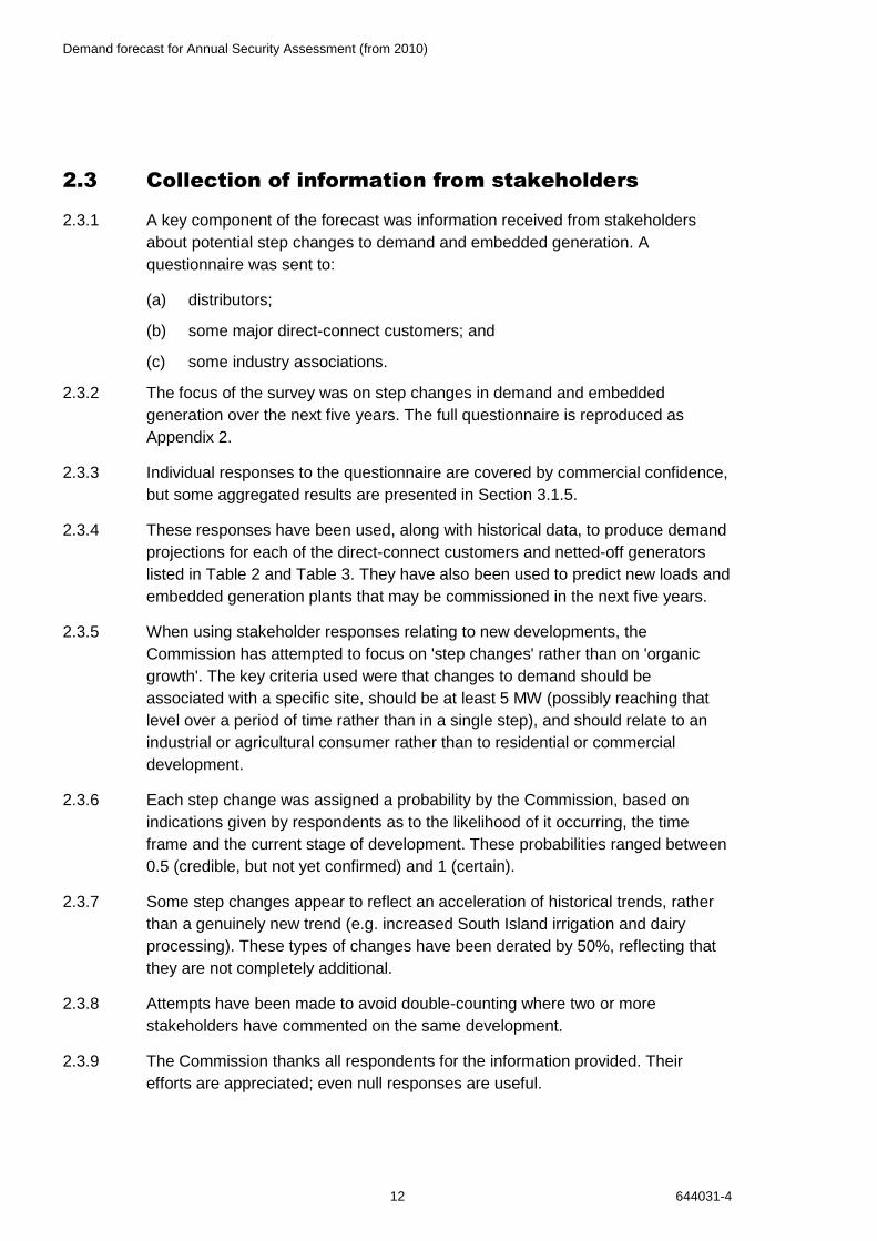
2.5.8 One set of projections is shown below, to illustrate the approach.
Figure 1: A sample of 20 projections of the residual demand component
2.6 Assembling the forecasts
2.6.1 The process used to produce the forecasts was to:
(a) produce many projections of annual energy demand over the 2011-15
period, by:
(i) projecting demand of selected existing direct-connect customers
(listed in Table 2), allowing for uncertainty;
(ii) projecting demand of significant new loads, allowing for uncertainty;
(iii) projecting generation of selected existing netted-off generators (listed
in Table 1) and new netted-off generators, allowing for uncertainty;
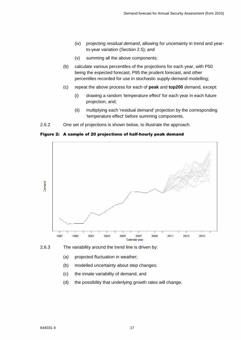
Demand forecast for Annual Security Assessment (from 2010)
644031-4 17
(iv) projecting residual demand, allowing for uncertainty in trend and year-
to-year variation (Section 2.5); and
(v) summing all the above components;
(b) calculate various percentiles of the projections for each year, with P50
being the expected forecast, P95 the prudent forecast, and other
percentiles recorded for use in stochastic supply-demand modelling;
(c) repeat the above process for each of peak and top200 demand, except:
(i) drawing a random 'temperature effect' for each year in each future
projection, and;
(ii) multiplying each 'residual demand' projection by the corresponding
'temperature effect' before summing components.
2.6.2 One set of projections is shown below, to illustrate the approach.
Figure 2: A sample of 20 projections of half-hourly peak demand
2.6.3 The variability around the trend line is driven by:
(a) projected fluctuation in weather;
(b) modelled uncertainty about step changes;
(c) the innate variability of demand; and
(d) the possibility that underlying growth rates will change.

Demand forecast for Annual Security Assessment (from 2010)
18 644031-4
2.7 Instantaneous peak forecasts
2.7.1 Electricity demand varies within each half-hour period. Published half-hour
demand figures are an average of data sampled at higher frequencies.
Accordingly, the instantaneous peak on any given day is greater than the half-
hourly peak (since the maximal value in the half-hour with highest demand will
always be greater than the average value in that half-hour). In New Zealand, the
difference can be over 100 MW.
2.7.2 For some purposes, half-hourly demand forecasts are adequate; in other
contexts, the instantaneous peak is more relevant. Accordingly, both types of
forecasts are provided in this report.
2.7.3 Instantaneous peak forecasts were derived by applying 'short-term variation
factors' to half-hourly peak forecasts, modelling the effect of within-half-hour
variation. The process used to derive these factors is described in the 2008
RENA demand forecast document.
2.7.4 Typically the process resulted in variation factors of about 1% (for expected
forecasts) or between 1% and 2% (for prudent forecasts). Different factors were
used for each region (NI, SI, and New Zealand overall).
2.7.5 Variation factors and instantaneous peak forecasts are presented in Section 3.5.

Demand forecast for Annual Security Assessment (from 2010)
644031-4 19
3. Results
3.1 Historical demand data
3.1.1 The historical demand data used to prepare the forecast are shown in Appendix
3. These series were derived from augmented Centralised Dataset information,
using the Gnash code in Appendix 1.
3.1.2 It should be expected that these demand figures will not be directly comparable
with those in other publications (such as the 2010 SOO), because of the
treatment of embedded generation, the calendar year (rather than March year)
basis, and some differences in region definitions. Naturally, the half-hourly peak
forecasts are not directly comparable with instantaneous peak forecasts
published elsewhere.
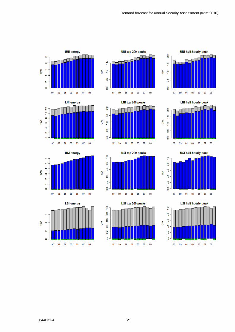
3.1.3 The same data are plotted in Figure 3. A note on interpretation: the position of
the top of each bar indicates the total demand less netted-off generation (this is
the quantity being forecast). The green portion below the y-axis is the embedded
generation component, including the plants listed in Table 3. The grey portion is
the industrial component, made up of the direct-connect customers listed in Table
2. Adding the blue and green portions together would yield the residual
component.
3.1.4 Two features are of particular interest:
(a) both peak and energy demand were low in 2008, 2009 and 2010, due
in part to a combination of:
(i) the 2008 dry winter and public conservation campaign, and
(ii) the 2008-09 demand reduction at the Tiwai smelter (caused by a
transformer failure).
Section 4.2 explores 2009-10 demand in more detail (in the context of
assessing the accuracy of earlier forecasts); and
(b) organic energy (as opposed to peak) growth in the North Island has been
low since 2006. The remainder of this section discusses this trend.

Demand forecast for Annual Security Assessment (from 2010)
20 644031-4
Figure 3: Historical demand data used in the forecast
Demand forecast for Annual Security Assessment (from 2010)
644031-4 21
Demand forecast for Annual Security Assessment (from 2010)
22 644031-4
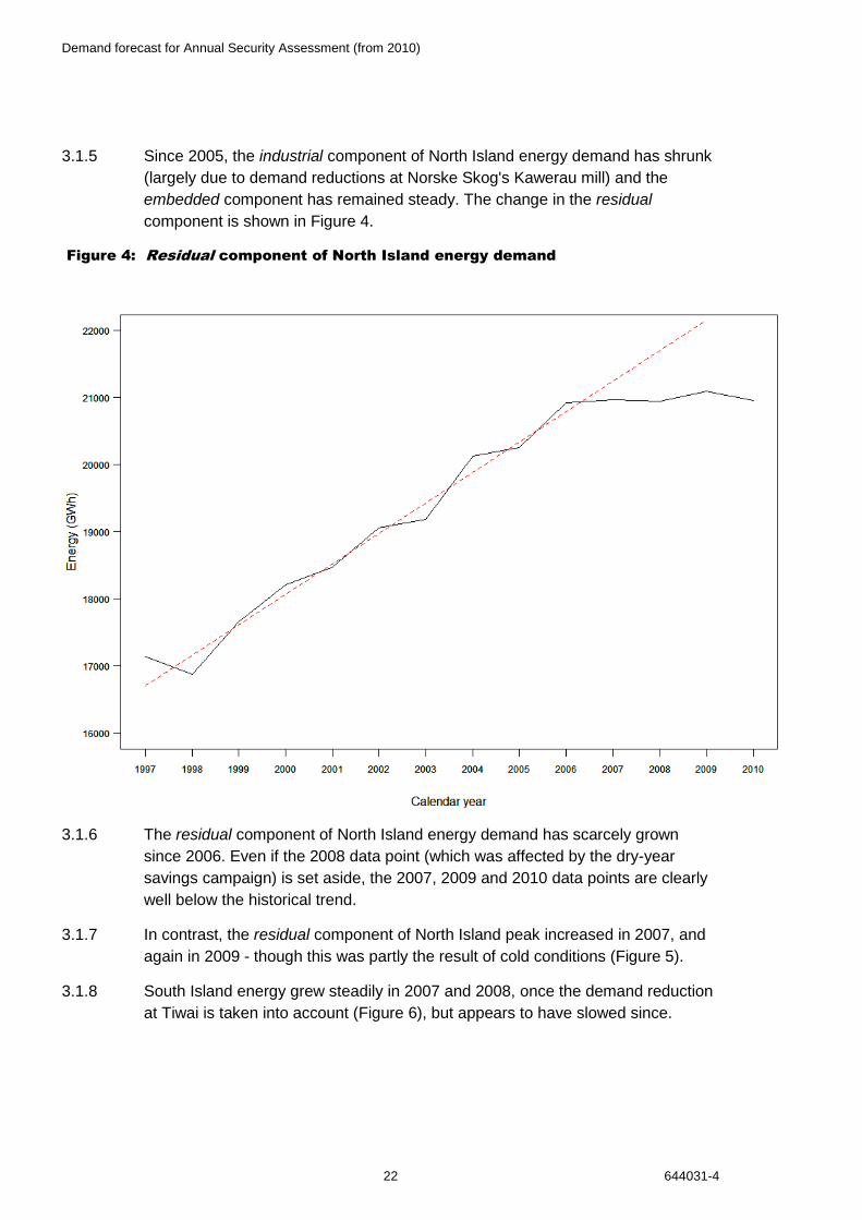
3.1.5 Since 2005, the industrial component of North Island energy demand has shrunk
(largely due to demand reductions at Norske Skog's Kawerau mill) and the
embedded component has remained steady. The change in the residual
component is shown in Figure 4.
Figure 4: Residual component of North Island energy demand
3.1.6 The residual component of North Island energy demand has scarcely grown
since 2006. Even if the 2008 data point (which was affected by the dry-year
savings campaign) is set aside, the 2007, 2009 and 2010 data points are clearly
well below the historical trend.
3.1.7 In contrast, the residual component of North Island peak increased in 2007, and
again in 2009 - though this was partly the result of cold conditions (Figure 5).
3.1.8 South Island energy grew steadily in 2007 and 2008, once the demand reduction
at Tiwai is taken into account (Figure 6), but appears to have slowed since.

Demand forecast for Annual Security Assessment (from 2010)
644031-4 23
Figure 5: Residual component of North Island peak demand
Figure 6: Residual component of South Island energy demand
Excludes Tiwai
2008 - affected by
savings campaign
2010 - mild winter
2009 - cold winter
Demand forecast for Annual Security Assessment (from 2010)
24 644031-4
3.1.9 The reasons why North Island energy growth has slowed since 2006 are not
clear. Some of the reasons could be:
(a) increased electricity efficiency;
(b) consumer response to rising electricity prices; and
(c) economic conditions.
3.1.10 However, at this stage there is no way of determining which of the above factors
has been most important.
3.1.11 The slowdown in demand growth has certainly not affected the whole country.
There have been substantial differences in recent demand growth rates between
regions of New Zealand (Table 4).
Table 4 Comparison of recent energy demand growth rates
(excluding industrial and embedded generation components)
Growth rate Regions
Highest
(over 5% p.a.)
West Coast
High
(2.5-3% p.a.)
Waikato, Bay of Plenty, South Canterbury
Average
(1.5-2% p.a.)
Auckland, Canterbury, Otago/Southland
Low
(less than 1.5%)
Central North Island, Hawkes Bay, Nelson/Marlborough, North
Isthmus/Northland, Taranaki, Wellington
Growth rates shown are based on the increase in demand from 2002-04 to 2007-09.
3.1.12 In some regions, the reasons for the observed trends are clear (e.g. dairy growth
in South Canterbury, dairy and mining on the West Coast). Others are not as
evident.
3.1.13 MED data suggests that the reduction in national energy demand growth rates
has been driven by the residential sector. According to the Energy Datafile21,
there has been substantial growth in commercial and agricultural electricity
demand in the last five years, but minimal growth in the residential sector. It is a
21
Energy Datafile, http://www.med.govt.nz/templates/MultipageDocumentTOC____43905.aspx, Table G.1

Demand forecast for Annual Security Assessment (from 2010)
644031-4 25
little hard to compare the MED figures on an 'apples vs apples' basis with those
presented here, but the result is interesting.
3.1.14 One can speculate about the extent to which electricity efficiency has helped to
restrain demand growth, and will continue to do so. According to EECA (pers.
comm.), some electricity efficiency measures that could have helped slow
demand growth over the last few years are:
(a) increased use of compact fluorescent light bulbs;
(b) replacement of traditional electric heaters with heat pumps;
(c) installation of efficient home appliances (such as whiteware and hot water
cylinders) under minimum energy performance standards (MEPS); and
(d) improvements in the industrial sector (perhaps lighting or motors).
3.1.15 All these measures (and more) will continue over the next few years, and are
expected to yield ongoing efficiency gains.
3.1.16 On the other hand, there are concerns about power-guzzling televisions,
replacement of gas and solid fuel heaters with electric heat pumps, and the
'takeback' effect (i.e. consumers responding to increased efficiency by using their
appliances more often).
3.1.17 The question for the forecaster (and the wider industry) is: will energy growth
over the next few years return to the ten-year trend, or will it continue at the
slower rate that has been seen since 2006? The base case forecasts in this
document effectively assume the former, and predict that electricity consumption
in 2011-15 will be substantially higher than in 2008-10.
3.1.18 A "hockey stick" sensitivity is also included, exploring the effect of a sustained
period of low growth (Section 6).
3.2 Demand questionnaire findings
3.2.1 This section describes the responses to the Commission's questionnaire about
potential step changes in demand and embedded generation (Section 2.3), to the
limited extent that confidentiality requirements allow.
3.2.2 Responses were received from a high proportion of questionnaire recipients. The
Commission wishes to thank all respondents.
3.2.3 In some cases the response was a simple 'no step changes expected', or the
step changes predicted did not fit the criteria for inclusion in the forecast, but
these responses were appreciated nonetheless.

Demand forecast for Annual Security Assessment (from 2010)
26 644031-4
3.2.4 Most respondents indicated that they wished the information provided to remain
confidential, and accordingly none of the responses will be published. However,
some qualitative comments about the nature of the responses are made below.
3.2.5 The following types of step changes were not used in the forecast:
(a) changes to generation that is not netted off the forecast, e.g. new wind
farms of at least 30 MW capacity or grid-connected geothermal
developments;
(b) changes of less than 5 MW;
(c) changes taking place after winter 2015;
(d) changes identified by the respondent as having a low probability; and
(e) changes to residential or commercial demand (which are intended to be
incorporated in the 'residual component' of demand, rather than modelled
separately as step changes).
3.2.6 About twenty changes remained after the above filters had been applied. As
noted in Section 2.3, each step change was assigned a probability and some
were derated as not fully additional.
3.2.7 The most significant changes over the period to 2015 relate to (in no particular
order):
(a) expected or potential production increases by major (grid-connected)
industrial consumers;
(b) new generation (small wind and hydro, embedded peakers)
(c) irrigation;
(d) mining; and
(e) new dairy processing facilities.
3.2.8 No single change was expected to have an effect of more than 20 MW.
3.2.9 Results were generally quite consistent with the 2009 survey. The 2008 survey
was more optimistic than either, featuring various new schemes throughout the
country, but economic conditions seem to have damped activity.

Demand forecast for Annual Security Assessment (from 2010)
644031-4 27
3.3 Temperature vs peak demand – results
3.3.1 The analysis of temperature vs peak demand is described in Section 2.4. This
section presents the 'temperature-corrected peaks' produced for each half-island
for each year from 1997 to 2010.
3.3.2 The analysis applies to the 'residual component' of demand only.
3.3.3 Plots of 'temperature-corrected vs actual' residual demand are shown below, for
each island (peak and top200), and each half-island (peak only). Generally,
accounting for temperature effects reduces the year-to-year variability of demand.
(The dashed series are more linear than the solid series.)
3.3.4 2006 is a good example of a year that was affected by a cold snap (for both
islands, the solid line is higher than the dashed; peak demand would have been
lower if not for cold conditions).
3.3.5 Winter 2008 was mild in the South Island and average in the North.
3.3.6 Winter 2009 was unusually cold in the North Island - with the most severe
temperature effect in the last decade - but average in the Upper South and mild
in the Lower South.
3.3.7 Winter 2010 was mild throughout the country.
Demand forecast for Annual Security Assessment (from 2010)
28 644031-4
Figure 7: Residual demand component averaged over top 200 peaks - actual vs
temperature-corrected

Demand forecast for Annual Security Assessment (from 2010)
644031-4 29
Figure 8: Residual demand component at half-hourly peak - actual vs
temperature-corrected
Demand forecast for Annual Security Assessment (from 2010)
30 644031-4

Demand forecast for Annual Security Assessment (from 2010)
644031-4 31

Demand forecast for Annual Security Assessment (from 2010)
32 644031-4
3.4 Forecasts
3.4.1 This section presents the forecasts of annual energy, half-hourly peak and
top200 (i.e. mean of the 200 highest half-hourly peaks).
3.4.2 As earlier noted, these forecasts are not directly comparable with those in other
publications (such as the 2010 SOO), because of the treatment of embedded
generation, the calendar year (rather than March year) basis, and some
differences in region definitions. Naturally, the half-hourly peak forecasts are not
directly comparable with instantaneous peak forecasts published elsewhere.
3.4.3 2010 energy figures (italic) are partially based on imputed data (since, at time of
writing, the 2010 year is not yet complete).
Table 5 Forecasts
Energy (GWh) Half-hourly peak (MW) Top200 (MW)
Region Year Expected Prudent Expected Prudent Expected Prudent
NZ 2004 37,150 6,022 5,859
2005 37,120 6,045 5,862
2006 37,598 6,329 6,076
2007 38,034 6,405 6,129
2008 37,912 6,185 5,970
2009 37,521 6,375 6,068
2010 38,429 6,232 6,029
2011 40,466 41,798 6,676 6,931 6,472 6,698
2012 41,239 42,655 6,800 7,065 6,591 6,827
2013 41,977 43,514 6,921 7,212 6,709 6,973
2014 42,702 44,532 7,027 7,344 6,826 7,115
2015 43,481 45,495 7,154 7,514 6,945 7,277
NI 2004 23,560 4,104 3,949
2005 23,541 4,070 3,928
2006 23,839 4,261 4,075
2007 23,909 4,335 4,093
2008 23,894 4,199 4,008
2009 24,050 4,402 4,167
2010 23,939 4,199 4,023
2011 25,309 26,367 4,520 4,713 4,338 4,511
2012 25,756 26,951 4,600 4,805 4,415 4,594
2013 26,229 27,502 4,685 4,914 4,502 4,695
2014 26,682 28,053 4,766 5,023 4,581 4,801
2015 27,141 28,734 4,855 5,144 4,670 4,913

Demand forecast for Annual Security Assessment (from 2010)
644031-4 33
Energy (GWh) Half-hourly peak (MW) Top200 (MW)
Region Year Expected Prudent Expected Prudent Expected Prudent
SI 2004 13,590 2,000 1,934
2005 13,579 2,017 1,970
2006 13,759 2,076 2,027
2007 14,125 2,113 2,065
2008 14,017 2,098 2,001
2009 13,471 1,988 1,947
2010 14,489 2,058 2,024
2011 15,145 15,444 2,195 2,267 2,150 2,227
2012 15,468 15,816 2,234 2,310 2,190 2,273
2013 15,739 16,131 2,264 2,350 2,224 2,314
2014 16,023 16,494 2,290 2,380 2,253 2,354
2015 16,321 16,874 2,322 2,424 2,287 2,402
UNI 2004 10,241 1,869 1,804
2005 10,321 1,901 1,819
2006 10,641 2,044 1,925
2007 10,730 2,043 1,929
2008 10,742 2,028 1,906
2009 10,656 2,083 1,986
2010 10,654 2,028 1,927
2011 11,418 12,058 2,145 2,270 2,046 2,133
2012 11,644 12,297 2,186 2,316 2,084 2,177
2013 11,860 12,615 2,229 2,368 2,123 2,227
2014 12,105 12,920 2,274 2,424 2,163 2,279
2015 12,369 13,222 2,321 2,487 2,210 2,335
LNI 2004 13,318 2,252 2,156
2005 13,220 2,200 2,124
2006 13,197 2,282 2,166
2007 13,178 2,318 2,177
2008 13,153 2,235 2,118
2009 13,394 2,339 2,198
2010 13,285 2,239 2,120
2011 13,909 14,382 2,416 2,537 2,302 2,394
2012 14,114 14,629 2,459 2,588 2,342 2,436
2013 14,385 14,956 2,508 2,646 2,389 2,495
2014 14,575 15,232 2,550 2,701 2,428 2,545
2015 14,782 15,542 2,592 2,759 2,470 2,600

Demand forecast for Annual Security Assessment (from 2010)
34 644031-4
Energy (GWh) Half-hourly peak (MW) Top200 (MW)
Region Year Expected Prudent Expected Prudent Expected Prudent
USI 2004 5,812 983 937
2005 5,925 1,004 968
2006 6,081 1,048 1,020
2007 6,173 1,060 1,029
2008 6,453 1,074 1,027
2009 6,455 1,046 1,019
2010 6,543 1,032 1,013
2011 6,899 7,126 1,109 1,170 1,083 1,138
2012 7,108 7,335 1,132 1,194 1,108 1,166
2013 7,311 7,582 1,154 1,225 1,130 1,192
2014 7,506 7,833 1,169 1,246 1,150 1,221
2015 7,720 8,109 1,192 1,276 1,176 1,254
LSI 2004 7,779 1,023 1,006
2005 7,654 1,030 1,008
2006 7,678 1,036 1,015
2007 7,952 1,061 1,045
2008 7,565 1,046 1,021
2009 7,015 985 976
2010 7,946 1,054 1,028
2011 8,249 8,376 1,103 1,153 1,063 1,115
2012 8,365 8,505 1,120 1,169 1,076 1,132
2013 8,442 8,602 1,130 1,182 1,086 1,142
2014 8,527 8,706 1,140 1,193 1,093 1,152
2015 8,615 8,815 1,153 1,207 1,102 1,166

Demand forecast for Annual Security Assessment (from 2010)
644031-4 35
Figure 9: Forecasts

Demand forecast for Annual Security Assessment (from 2010)
36 644031-4
Demand forecast for Annual Security Assessment (from 2010)
644031-4 37

Demand forecast for Annual Security Assessment (from 2010)
38 644031-4

Demand forecast for Annual Security Assessment (from 2010)
644031-4 39
3.4.4 For 2011, the national energy forecasts are 40,466 GWh (expected, P50) and
41,798 GWh (prudent, P95). These forecasts represent annual growth of 1.6% or
2.4% since 2007, in which the energy demand was 38,034 GWh.
3.4.5 The expected rate of energy growth from 2011 to 2015 is 2.1%.
3.4.6 For 2011, the national half-hourly peak forecasts are 6,676 MW (expected, P50)
and 6,931 MW (prudent, P95). These forecasts represent annual growth of 1.0%
(expected) or 2.0% (prudent) since 2007, in which the half-hourly peak was
6,405 MW.
3.4.7 The expected rate of peak growth from 2011 to 2015 is 2.0%.
3.4.8 Expected national energy and peak growth rates are quite similar (2.1% vs 2.0%
after 2011).
3.4.9 Energy growth is predicted to be very similar across the two islands. Peak growth
is expected to be higher in the North Island (2.2%) than the South Island (1.7%).
Demand forecast for Annual Security Assessment (from 2010)
40 644031-4
3.5 Instantaneous peak forecasts
3.5.1 This section gives the results of the analysis of within-half-hour variation
described in Section 2.7, and presents forecasts of instantaneous peak demand.
3.5.2 Instantaneous peak forecasts were derived by applying 'short-term variation
factors' to half-hourly peak forecasts, modelling the effect of within-half-hour
variation.
Table 6 Short-term variation factors, as used to produce
instantaneous peak forecasts
Region Variation factor – expected forecast
Variation factor – prudent forecast
All NZ 0.8% 1.3%
North Island 1.0% 1.9%
South Island 1.0% 1.4%
3.5.3 For example, the expected forecasts of instantaneous peak for the North Island
are calculated by adding 1.0% to the expected forecasts of half-hourly peak.
3.5.4 The variation factors for the expected forecast are considerably lower than those
for the prudent forecast:
(a) the expected forecast variation factors are based on mean ratios of annual
instantaneous peak to annual half-hourly peak from 2002 to 2006. For New
Zealand as a whole, these ratios have ranged from 1.0056 to 1.0096, with a
mean of 1.008, hence the 0.8% variation factor;
(b) the prudent forecast variation factors are based on an analysis of the ratio
of daily instantaneous peak to daily half-hourly peak on high-demand winter
days from 2002 to 2006. On some days, this ratio has been as high as
1.016 for New Zealand – but this is a rare event, unlikely to occur on the
same day as the annual half-hourly peak. Accordingly, the variation factors
used are based on the 90th percentile of the sample of ratios, rather than
the maximum. For New Zealand this is 1.013, hence the 1.3% variation
factor.
3.5.5 For New Zealand as a whole, in 2011, this analysis indicates a margin of 90 MW
between the half-hourly and instantaneous prudent peak forecasts.
3.5.6 The resulting instantaneous peak forecasts are shown below, for New Zealand as
a whole and for each island.
Demand forecast for Annual Security Assessment (from 2010)
644031-4 41
Table 7 Instantaneous peak forecasts
Instantaneous peak (MW)
Region Year Expected Prudent
NZ
2011 6,730 7,021
2012 6,855 7,157
2013 6,976 7,305
2014 7,083 7,440
2015 7,211 7,612
NI
2011 4,565 4,803
2012 4,646 4,896
2013 4,732 5,007
2014 4,814 5,118
2015 4,904 5,242
SI
2011 2,217 2,299
2012 2,256 2,342
2013 2,287 2,383
2014 2,312 2,413
2015 2,345 2,458
3.6 Changes since 2008
3.6.1 This section compares the demand forecasts in this document with the
predictions made in the 2008 RENA demand forecast and the demand
assumptions used in the 2009 ASA.22
3.6.2 Table 8 and Table 9 compare the 2008, 2009 and 2010 energy forecasts;
Table 10 and Table 11 compare peak forecasts. (The 2008 and 2009 documents
did not include top200 forecasts.)
3.6.3 Both energy and peak forecasts have dropped substantially since 2008
(driven mainly by low 2009 and 2010 actuals).
22
The 2009 ASA used an update of the 2008 RENA demand forecast incorporating new survey information,
rather than a completely new demand forecast.

Demand forecast for Annual Security Assessment (from 2010)
42 644031-4
Table 8: Comparison between expected energy demand forecasts
Year 2008 RENA forecast
2009 ASA demand assumptions
2010 ASA forecast
2011 42,415 42,315 40,466
2012 43,249 43,149 41,238
2013 44,058 43,958 41,976
Table 9: Comparison between prudent energy demand forecasts
Year 2008 RENA forecast
2009 ASA demand assumptions
2010 ASA forecast
2011 43,496 43,396 41,798
2012 44,571 44,471 42,655
2013 45,602 45,502 43,514
Table 10: Comparison between expected halfhourly peak demand forecasts
Year 2008 RENA forecast
2009 ASA demand assumptions
2010 ASA forecast
2011 6,920 6,895 6,676
2012 7,047 7,022 6,800
2013 7,169 7,144 6,920
Table 11: Comparison between prudent halfhourly peak demand forecasts
Year 2008 RENA forecast
2009 ASA demand assumptions
2010 ASA forecast
2011 7,103 7,078 6,931
2012 7,266 7,241 7,065
2013 7,435 7,410 7,211
Demand forecast for Annual Security Assessment (from 2010)
644031-4 43
Figure 10: Comparison between expected forecasts
37,000
38,000
39,000
40,000
41,000
42,000
43,000
44,000
45,000
2006 2007 2008 2009 2010 2011 2012 2013
An
nu
al
en
erg
y (
GW
h)
.
2008 RENA forecast
2009 ASA demand
assumptions
2010 ASA forecast
2007 actual
6,300
6,400
6,500
6,600
6,700
6,800
6,900
7,000
7,100
7,200
7,300
2006 2007 2008 2009 2010 2011 2012 2013
Peak (
MW
)
.
2008 RENA forecast
2009 ASA demand
assumptions
2010 ASA forecast
2007 actual
Demand forecast for Annual Security Assessment (from 2010)
44 644031-4
3.7 Caveats
3.7.1 This section lists some concerns about the forecasts.
3.7.2 The forecasts do not include econometric predictors. It is fairly clear that the state
of the economy has slowed demand growth since 2008 (see sections 3.1, 4.2).
There is further economic trouble ahead - NZIER, for instance, predicts a
"slowing recovery" with "a weak patch in late 2010 and early 2011" and warns of
impending collapse in the non-residential construction sector.23 An implication is
that electricity demand growth may be lower than forecast.
3.7.3 It would be possible to model this dynamic by adding econometric predictors to
future forecasts, but this would only be useful to the extent that the state of the
economy can be predicted years in advance - a notoriously difficult problem.
3.7.4 The forecasts do not consider technological or market step changes that may
occur in future. An example would be the introduction of critical peak pricing
tariffs for residential consumers with smart meters, which would have the
potential to slow peak growth. It has also been suggested that the introduction of
plug-in electric vehicles may increase demand, but it is very unlikely that there
will be significant uptake before 2015.
3.7.5 The forecasts do not specifically model increases in electricity efficiency or an
increased focus on conservation among residential customers. These effects
have slowed demand growth in recent years (Section 3.1) and will continue to do
so - but it is not clear to what extent.
3.7.6 It may be possible to add statistics on efficient appliance sales (heat pumps,
CFLs, whiteware) to future forecasts, though obtaining the relevant data is not
straightforward.
3.7.7 The forecasts do not consider changes in how load control is used. The South
Island load controller has helped to manage peak in the winters of 2009 and
2010 (Section 4.2) and there are opportunities for future cooperation of this sort.
3.7.8 On the other hand, some parties have suggested that the use of load control to
manage peaks may decline in future (because there may not be appropriate
incentives for distributors to do so, or because the load may be controlled for
other purposes e.g. by retailers via smart meters, or because ageing ripple
control systems are not being maintained).
3.7.9 Some of these uncertainties can, perhaps, be addressed by improving the
forecasting methodology; others will only be resolved by the passage of time.
23
http://www.nzier.org.nz/Site/News/media_releases/media_releases_list.aspx
Demand forecast for Annual Security Assessment (from 2010)
644031-4 45
4. Validation
4.1 Introduction
4.1.1 This section describes the analysis carried out to validate the forecasts in this
document.
4.1.2 There are three main approaches to validation:
(a) comparing predicted demand to recent historical demand;
(b) comparing predicted demand to actual demand, once the actual demand
data become available; and
(c) out of sample forecasting – carrying out forecasts for years that have
already occurred, based on the information that would have been available
in advance, and comparing these 'out of sample forecasts' with actual
demand.
4.1.3 On (a), the near-future growth rates predicted in the 'expected' forecasts are
broadly consistent with growth rates in the last decade.
4.1.4 On (b), comparisons of predictions for 2009-10 in the 2008 RENA demand
forecast with actual 2009-10 demand are provided in Section 4.2.
4.1.5 In theory, predictions for 2008 could also be compared with actual 2008 demand.
However, electricity demand in 2008 was depressed by the dry year and resulting
public conservation campaign, so this has not been done.
4.1.6 On (c), an out of sample analysis was carried out as part of the 2007 RENA
demand forecast and has not been repeated this year.

Demand forecast for Annual Security Assessment (from 2010)
46 644031-4
4.2 Validation of the predictions for 2009 and 2010
4.2.1 Actual energy and peak demand figures for 2009, and peak demand figures for
2010, are now available. In this section, these actuals are compared with the
predictions for 2009 in the 2008 RENA demand forecast.
4.2.2 The aim of the analysis is to gain information about the performance of the
demand forecasting methodology over very short time scales.
4.2.3 We first consider half-hourly peak predictions for 2009.
Table 12 Predicted 2009 half-hourly peaks vs actual values
Region Actual peak (MW)
Expected forecast (MW)
Prudent forecast (MW)
Actual minus expected (MW, %)
NZ (*) 6,374 6,646 6,791 -272 (-4.1%)
NI 4,402 4,494 4,626 -92 (- 2.0%)
SI (*) 1,988 2,211 2,270 -223 (-10.0%)
UNI 2,082 2,111 2,235 -29 (-1.4%)
LNI 2,338 2,412 2,505 -74 (-3.1%)
USI 1,045 1,131 1,180 -86 (-7.6%)
LSI (*) 984 1,096 1,135 -112 (-10.2%)
(*) - Affected by reduction in Tiwai consumption following transformer failure in 2008
Figures shown will not correspond exactly to figures published elsewhere, due to different
treatment of netted-off generation.
4.2.4 All peak demand forecasts for 2009 in the 2008 RENA forecast were too high.
4.2.5 New Zealand peak demand was 270 MW (4%) below the expected forecast.
In part this was a consequence of unexpectedly low demand at the NZAS
aluminium smelter (following a transformer failure in 2008), which led to Lower
South Island peak being 110 MW (10%) below forecast.
4.2.6 However, peak forecasts were also too high for regions that do not include the
Tiwai smelter.

Demand forecast for Annual Security Assessment (from 2010)
644031-4 47
4.2.7 North Island peak demand was 90 MW (2%) below the expected forecast, largely
due to reductions in the industrial component of peak - the residual and
embedded components were accurately predicted. This result should be taken in
context of a cold North Island winter (Section 3.3) - had temperatures been
milder, the gap between actual and expected demand would have been higher.
4.2.8 Upper South Island peak demand was 86 MW (7.6%) below the expected
forecast, despite average weather in mid-late winter.24 We believe this was a
result of several factors, including:
(a) the introduction of the Upper South Island load controller in March 200925,
which has been estimated to have reduced peak load by 30 MW over the
winter26;
(b) the economic downturn; and
(c) energy efficiency and fuel switching.
24
South Island weather was unusually cold in early winter, but this period did not set the annual island peak
because Tiwai demand was still low.
25 http://www.oriongroup.co.nz/load-management/Upper-south-island-load-management.aspx
26 http://www.oriongroup.co.nz/downloads/USI_Load_Management_annual_progress_reportFeb10.pdf

Demand forecast for Annual Security Assessment (from 2010)
48 644031-4
4.2.9 We next consider half-hourly peak predictions for 2010.
Table 13 Predicted 2010 half-hourly peaks vs actual values
Region Actual peak (MW)
Expected forecast (MW)
Prudent forecast (MW)
Actual minus expected (MW, %)
NZ 6,232 6,796 6,954 -564 (-8.3%)
NI 4,199 4,607 4,751 -408 (-8.9%)
SI 2,058 2,248 2,309 -190 (-8.5%)
UNI 2,028 2,182 2,309 -154 (-7.1%)
LNI 2,239 2,457 2,555 -218 (-8.9%)
USI 1,032 1,154 1,205 -122 (-10.6%)
LSI 1,054 1,111 1,153 -57 (-5.1%)
(*) - Slightly affected by reduction in Tiwai consumption
Figures shown will not correspond exactly to figures published elsewhere, due to different
treatment of netted-off generation.
4.2.10 All peak demand forecasts for 2010 in the 2008 RENA forecast were much too
high.
4.2.11 We attribute this to a combination of several factors, including:
(a) a mild winter;
(b) Tiwai demand still being slightly below normal;
(c) reduced demand by North Island industrial consumers at peak times;
(d) the effect of the Upper South Island load controller;
(e) the economic downturn; and
(f) energy efficiency and fuel switching.
Demand forecast for Annual Security Assessment (from 2010)
644031-4 49
4.2.12 We next consider energy predictions for 2009.
Table 14 Predicted 2009 energy vs actual values
Region Actual energy (GWh)
Expected forecast (GWh)
Prudent forecast (GWh)
Difference between actual and expected
(GWh)
NZ (*) 37,520 40,557 41,312 (3,037) - 7.5%
NI 24,050 25,471 26,079 (1,421) - 5.6%
SI (*) 13,470 15,082 15,535 (1,612) - 10.7%
UNI 10,656 11,488 11,830 (832) - 7.2%
LNI 13,393 13,989 14,308 (596) - 4.3%
USI 6,455 6,818 6,988 (363) - 5.3%
LSI (*) 7,015 8,264 8,404 (1,249) - 15.1%
(*) - Affected by reduction in Tiwai consumption following transformer failure in 2008
Figures shown will not correspond exactly to figures published elsewhere, due to different
treatment of netted-off generation.
4.2.13 All energy demand forecasts for 2009 in the 2008 RENA forecast were much too
high.
4.2.14 New Zealand energy demand was 3,000 GWh (7.5%) below the expected
forecast. In part this was a consequence of low Tiwai demand, which led to
Lower South Island energy demand being 1,200 GWh (15%) below forecast.
4.2.15 However, energy forecasts were also too high for regions that do not include the
Tiwai smelter. North Island energy demand was 1,400 GWh (5.5%) below the
expected forecast, and Upper South Island energy demand was 350 GWh (5%)
below the forecast.
4.2.16 The North Island over-forecasts (of both energy and peak) were largely driven by
overestimation of the residual component of demand; the Upper South Island
over-forecasts were also affected by overestimation of the industrial component.

Demand forecast for Annual Security Assessment (from 2010)
50 644031-4
4.2.17 We have not included a comparison of energy predictions for 2010 with actuals,
because the 2010 year is not complete. However, based on data for Jan-Sep
2010, it is clear that actuals will be much lower than predictions for all areas.
4.2.18 We conclude that:
(a) peak and energy demand in 2009 and 2010 were lower than expected,
even once the effects of low Tiwai demand are taken into account;
(b) for energy, this is a continuation of a trend that has been in progress since
2006 (Section 3.1); and
(c) the reasons are not clear, but may include some combination of low
economic growth, consumer response to rising prices, the introduction of
the Upper South Island load controller, and increases in electricity
efficiency.
4.2.19 It remains to be seen how accurate the predictions in this report will be. There are
clear risks that:
(a) recent slowdowns in demand growth are only a short-term 'blip', and will
soon be reversed by a period of rapid growth (in which case the present
forecast may be too low); OR
(b) recent slowdowns in demand growth reflect a new underlying trend, and will
continue over the next few years (in which case the present forecast may
be too high).
Demand forecast for Annual Security Assessment (from 2010)
644031-4 51
5. Comparisons with other published forecasts
5.1 Introduction
5.1.1 This section compares the forecasts presented in this document with the 2010
GPA demand forecasts.27
5.1.2 The 2007 RENA forecast document also included comparisons with:
(a) the half-hourly peak forecasts in Transpower's System Security Forecast
(SSF), as published in December 2006;28 and
(b) the energy forecast in the Ministry of Economic Development's Energy
Outlook to 2030 (Outlook), as published in November 2006,29
but these comparisons have not been repeated this year.
5.1.3 It should be noted that the forecasts listed above are intended to be long-term
predictions, with the SSF spanning ten years and the GPAs and Outlook
considerably longer. They were not designed to be accurate over the short term
(1-2 years).
5.2 The 2010 GPA forecasts
5.2.1 The 2010 GPAs include regional, island and national forecasts of energy and
half-hourly peak, extending to 2040 and beyond.
5.2.2 The GPA energy forecast used a top-down econometric approach, first identifying
the relationship between national demand growth and exogenous econometric
variables (such as GDP and population) then using this relationship to predict
growth in demand based on projections of the exogenous econometric variables.
The model was somewhat bottom-up, with separate sub models for residential,
industrial/commercial, and Tiwai demand.
5.2.3 Island- and region-level energy demand was predicted by applying an allocation
method to the national forecast, rather than by creating separate regional models
(because of the limitations of the historical econometric data).
5.2.4 The GPA 'Prudent and Expected' peak demand forecasts were a compromise
between a top-down statistical approach and a top-down econometric approach.
The predicted long-run growth in peak demand was driven by energy demand
27
http://www.ea.govt.nz/industry/modelling/demand-forecasting/, http://www.ea.govt.nz/industry/ec-
archive/soo/2010-soo/
28 www.transpower.co.nz/?id=4801
29 http://www.med.govt.nz/templates/MultipageDocumentTOC____21862.aspx

Demand forecast for Annual Security Assessment (from 2010)
52 644031-4
growth (and hence by econometric forecasts), but short-term growth was
adjusted upwards to match recent historical growth rates where these exceeded
projected energy growth. Predicted variability on all time scales was driven by
observed historical variability. Weather data were not used; weather-based
variability was effectively 'rolled in' with all other sources of demand variability.
5.2.5 Participant information about expected load shifts was used sparingly in the GPA
forecasts, in cases where it could be demonstrated to a high standard of
confidence that a change will occur and that it would be of a significant size
compared to the underlying load.
5.2.6 A 'high growth' scenario of energy demand has been extracted, using a 5% POE
criterion. 'Prudent' forecasts of peak demand were produced, though they were
based on a 10% POE criterion, rather than the 5% POE prudent forecasts
presented in this work. These prudent peak forecasts incorporated an allowance
for the possibility that peak would grow substantially faster than energy over the
next few years, which was thought to be a significant risk.
5.2.7 Comparisons between the medium-term forecasts in this document and the first
few years of the GPA forecasts are shown on the following page.
5.2.8 The main difficulty in making meaningful comparisons relates to the different
treatment of netted-off generation. The GPA forecasts are 'net of embedded
generation'. It would be expected that this would lead to a different baseline, with
(for example) Tararua 1 and 2 netted off – by comparison, in this work Tararua 1
and 2 are not netted off, but Glenbrook cogeneration is.
5.2.9 Accordingly, the comparisons relate to growth rates since 2007 rather than
absolute levels of demand. This goes some way towards resolving the problem of
inconsistent baselines.
5.2.10 Another complication was that the GPA energy forecasts are for 'March years',
i.e. the label 2007 indicates the period from 1 April 2006 to 31 March 2007.
These have been converted to calendar years by approximating the demand in
calendar year X as 0.25 times the demand in March year X plus 0.75 times the
demand in March year X+1.

Demand forecast for Annual Security Assessment (from 2010)
644031-4 53
Figure 11: Comparison with GPA energy forecasts (relative to 2007)
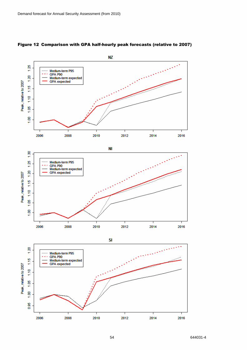
Demand forecast for Annual Security Assessment (from 2010)
54 644031-4
Figure 12 Comparison with GPA half-hourly peak forecasts (relative to 2007)

Demand forecast for Annual Security Assessment (from 2010)
644031-4 55
5.2.11 In terms of North Island energy, the GPA forecast is very similar to the medium-
term forecast for 2011, but grows more rapidly over 2012-15.
5.2.12 In terms of South Island energy, the two forecasts are very similar over 2011-15.
5.2.13 In terms of peak, the GPA forecasts are much higher than the medium-term
forecasts, for both islands over 2011-15. (This is mainly because the GPA
forecast does not take account of the low peak demand observed in 2009 and
2010. The GPA forecast is also more bullish about increases to specific
agricultural and industrial loads.)

Demand forecast for Annual Security Assessment (from 2010)
56 644031-4
6. Low growth ('hockey stick') sensitivity
6.1 Rationale
6.1.1 As set out in Section 3.1, North Island energy growth was reasonably rapid over
1997-2006 but much slower over 2007-10. Several possible causes have been
suggested, but it is not clear which (if any) is the primary driver of the change, nor
whether the period of slow growth will continue.
6.1.2 South Island energy growth, and peak demand growth in both islands, have also
slowed in the last couple of years.
6.1.3 The 'base case' forecasts in this document implicitly assume that growth over the
next few years will return to the ten-year trend, and hence predict that demand in
2011-15 will be substantially higher than in 2008-10.
6.1.4 This section sets out a 'hockey stick'
sensitivity in which it is assumed that
the slower rate of growth observed
since 2006 will continue over 2011-15.
6.1.5 The 'hockey stick' indicates a
piecewise trend, with a long period of
rapid growth followed by a shorter
period of slow growth.
6.1.6 It may be appropriate to use this as
the basis for a 'low energy growth'
sensitivity in the 2010 ASA.
6.2 Assumptions
6.2.1 The methodology used in the 'hockey stick' sensitivity is the same as in the 'base
case' energy forecast, except that the linear regression (in log space) of Section
2.5 becomes a piecewise linear fit (also in log space).
6.2.2 The join between the two pieces is between the years 2006 and 2007.
6.3 Results
6.3.1 The 'hockey stick' predictions are provided in Table 15, Figure 13, Table 16 and
Figure 14.
2006

Demand forecast for Annual Security Assessment (from 2010)
644031-4 57
Table 15 Energy forecasts - 'hockey stick' sensitivity
Energy (GWh)
Region Year Expected Prudent
NZ 2004 37,150
2005 37,120
2006 37,598
2007 38,034
2008 37,912
2009 37,521
2010 38,429
2011 39,026 39,689
2012 39,245 40,072
2013 39,580 40,654
2014 39,817 41,156
2015 40,018 41,760
NI 2004 23,560
2005 23,541
2006 23,839
2007 23,909
2008 23,894
2009 24,050
2010 23,939
2011 24,089 24,613
2012 24,116 24,736
2013 24,196 25,008
2014 24,198 25,202
2015 24,250 25,393
SI 2004 13,590
2005 13,579
2006 13,759
2007 14,125
2008 14,017
2009 13,471
2010 14,489
2011 14,923 15,197
2012 15,149 15,513
2013 15,330 15,772
2014 15,521 16,115
2015 15,745 16,435

Demand forecast for Annual Security Assessment (from 2010)
58 644031-4
Figure 13 Energy forecasts - 'hockey stick' sensitivity

Demand forecast for Annual Security Assessment (from 2010)
644031-4 59
Table 16 Peak forecasts - 'hockey stick' sensitivity
Half-hourly peak (MW)
Region Year Expected Prudent
NZ 2004 6,022
2005 6,045
2006 6,329
2007 6,405
2008 6,185
2009 6,375
2010 6,232
2011 6,482 6,693
2012 6,518 6,760
2013 6,595 6,851
2014 6,630 6,937
2015 6,667 7,062
NI 2004 4,104
2005 4,070
2006 4,261
2007 4,335
2008 4,199
2009 4,402
2010 4,199
2011 4,374 4,543
2012 4,400 4,596
2013 4,440 4,661
2014 4,460 4,732
2015 4,504 4,789
SI 2004 2,000
2005 2,017
2006 2,076
2007 2,113
2008 2,098
2009 1,988
2010 2,058
2011 2,132 2,186
2012 2,151 2,210
2013 2,164 2,230
2014 2,167 2,248
2015 2,179 2,282
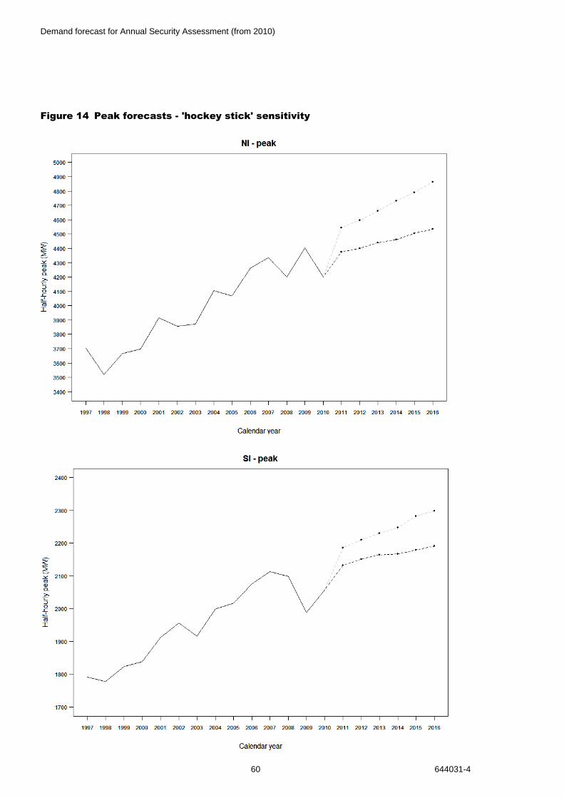
Demand forecast for Annual Security Assessment (from 2010)
60 644031-4
Figure 14 Peak forecasts - 'hockey stick' sensitivity

Demand forecast for Annual Security Assessment (from 2010)
644031-4 61
6.3.2 For 2011, the national energy forecasts are 39,026 GWh (expected, P50) and
39,689 GWh (prudent, P95). These forecasts represent annual growth of 0.6% or
1.1% since 2007, in which energy demand was 38,034 GWh.
6.3.3 The expected rate of energy growth from 2011 to 2015 is 1.3%.
6.3.4 North Island energy growth is much slower than South Island - with annual
growth of 0.8% and 2.0% respectively over the 2011-2015 period.
6.3.5 For 2011, the national half-hourly peak forecasts are 6,482 MW (expected, P50)
and 6,693 MW (prudent, P95). These forecasts represent annual growth of 0.3%
or 1.1% since 2007, in which peak demand was 6,405 MW.
6.3.6 The expected rate of peak growth from 2011 to 2015 is 1.3%.
6.3.7 North Island peak growth is slightly faster than South Island - with annual growth
of 1.3% and 1.1% respectively over the 2011-2015 period.

Demand forecast for Annual Security Assessment (from 2010)
62 644031-4
Appendices
Appendix 1 Gnash script used to produce the half-hourly demand
dataset 63
Appendix 2 Demand and embedded generation survey 66
Appendix 3 Historical demand data 68

Demand forecast for Annual Security Assessment (from 2010)
644031-4 63
Appendix 1 Gnash script used to produce the half-hourly demand dataset
%%%%%%%%%%%%%%%%%%%%%%%%%%%%%%%%%%%%%%%%%%%%%%%%%%%%%%%%%%%%%%%%%
% Gnash code to produce data for the Security of Supply Demand Forecast.
%
% Consistent with Gnash as of Oct 2010.
%
% Be aware that the Gnash data change without notice - series names, series contents, data gaps...
% Whenever this code is reused it will therefore be necessary to check the contents quite thoroughly.
% If in doubt, contact Brian Bull ([email protected]).
%
set dump.aux.provenance=F
set dump.aux.titles=F
%
%%%%%%%%%%%%%%%%%%%%%%%%%%%%%%%%%%%%%%%%%%%%%%%%%%%%%%%%%%%%%%%%%
%
% UNI
%
calculate uni_net_load = mergeadd(NI.BOMBAY.33KV, NI.BOMBAY.110KV, NI.Glenbrook.T4T5.Nett,
NI.Glenbrook.T6.Nett, NI.MANGERE.CITY, NI.MANGERE.STEELMILL, NI.OTAHUHU, NI.PAKURANGA, NI.PENROSE.22KV,
NI.PENROSE.33KV.A, NI.PENROSE.33KV.B, NI.PENROSE.110KV, NI.MOUNTROSKILL.22KV, NI.MOUNTROSKILL.110KV,
NI.TAKANINI, NI.WIRI, NI.ALBANY.33KV, NI.ALBANY.110KV, NI.BREAMBAY, NI.DARGAVILLE, NI.HENDERSON,
NI.HEPBURN.AUCKLAND, NI.HEPBURN.WAITEMATA, NI.KENSINGTON, NI.KAIKOHE, NI.KAITAIA.33KV, NI.MARSDEN, NI.MEREMERE,
NI.MAUNGATAPERE, NI.MAUNGATUROTO, NI.SILVERDALE.EXPORT, NI.WELLSFORD) - zpad(ni.kaikohe.import)
%
% Including the following major loads / embeddeds (positive is demand, negative is generation):
%
calculate uni_glenbrook = NI.Glenbrook.T4T5.Nett + NI.Glenbrook.T6.Nett
calculate uni_marsden_point = NI.BreamBay
calculate uni_pacific_steel = NI.MANGERE.STEELMILL
%
%%%%%%%%%%%%%%%%%%%%%%%%%%%%%%%%%%%%%%%%%%%%%%%%%%%%%%%%%%%%%%%%%
%
% USI
%
calculate usi_net_load = mergeadd(SI.CAIRNBRAE, SI.ADDINGTON.11KV.NETT.a, SI.ADDINGTON.66KV.NETT.a,
SI.ASHBURTON.33KV, SI.ASHBURTON.66KV.EXPORT, SI.ASHLEY, SI.BROMLEY.11KV, SI.BROMLEY.66KV, SI.COLERIDGE,
SI.CULVERDEN, SI.HORORATA.33KV, SI.HORORATA.66KV, SI.ISLINGTON, SI.ISLINGTON.HALSWELL, SI.KAIAPOI, SI.KAIKOURA,
SI.PAPANUI.11KV, SI.PAPANUI.66KV, SI.SOUTHBROOK.33KV, SI.SPRINGSTON.33KV, SI.SPRINGSTON.66KV.EXPORT,

Demand forecast for Annual Security Assessment (from 2010)
64 644031-4
SI.WAIPARA, SI.WAIPARA.66KV, SI.BLENHEIM, SI.KIKIWA, SI.MURCHISON, SI.MOTUEKA, SI.MOTUPIPI.33KV,
SI.MOTUPIPI.66KV, SI.STOKE, SI.ARAHURA.Export, SI.ARTHURSPASS, SI.CASTLEHILL, SI.DOBSON.export,
SI.GREYMOUTH.EXPORT, SI.HOKITIKA, SI.KUMARA.EXPORT, SI.WESTPORT.OROWAITI.CODE1, SI.WESTPORT.OROWAITI.CODE2,
SI.OTIRA.NZR, SI.REEFTON.EXPORT, SI.WESTPORT.ROBERTSON.export, SI.WAIMANGAROA, SI.WESTPORT, SI.TEMUKA.11KV,
SI.TEMUKA.33KV, SI.ALBURY.export, SI.TIMARU, SI.TEKAPO, SI.Reefton.110KV.Code1, SI.Reefton.110KV.Code2,
SI.Middleton.code1, si.atarau, si.middleton.code4) - zpad(SI.Ashburton.66KV.Import) - zpad(GEN.Hydro.Highbank)
- zpad(SI.KUMARA.IMPORT)
%
% Including the following major loads / embeddeds (positive is demand, negative is generation):
%
calculate usi_highbank = -(Gen.Hydro.Highbank)
%
%%%%%%%%%%%%%%%%%%%%%%%%%%%%%%%%%%%%%%%%%%%%%%%%%%%%%%%%%%%%%%%%%
%
% LNI
%
calculate lni_net_load = mergeadd(NI.EDGECUMBE, NI.KAWERAU.TOWN.EXPORT, NI.KAWERAU.TASMAN.C112,
NI.KAWERAU.TASMAN.C113, NI.MATAHINA, NI.MOUNTMAUNGANUI.11KV, NI.MOUNTMAUNGANUI.33KV, NI.OWHATA,
NI.ROTORUA.11KV.EXPORT, NI.ROTORUA.33KV.NETT, NI.TAURANGA.11KV, NI.TAURANGA.33KV.EXPORT, NI.TEKAHA, NI.TEMATAI,
NI.TARUKENGA, NI.WAIOTAHI, NI.BUNNYTHORPE.33KV.EXPORT, NI.Bunnythorpe.NZR.P1P2Nett.Active.Export, NI.BRUNSWICK,
NI.DANNEVIRKE, NI.LINTON.EXPORT, NI.MANGAMAIRE, NI.MANGAHAO, NI.MARTON, NI.MATAROA, NI.NATIONALPARK,
NI.OHAKUNE.A, NI.OHAKUNE.B, NI.ONGARUE.EXPORT, NI.TOKAANU, NI.TANGIWAI.KARIOI,
NI.TANGIWAI.NZR.P1P2Nett.Active.Export, NI.WOODVILLE, NI.WANGANUI, NI.WAIPAWA, NI.FERNHILL, NI.GISBORNE.11KV,
NI.GISBORNE.50KV, NI.REDCLYFFE, NI.TOKOMARUBAY, NI.TUAI, NI.WHIRINAKI.PP, NI.WAIROA.11KV.EXPORT,
NI.WAIROA.50KV, NI.WHAKATU, NI.CARRINGTON.11KV, NI.CARRINGTON.33KV, NI.HUIRANGI, NI.Hawera.110KV.Export,
NI.Hawera.110KV.Whareroa.Export, NI.Hawera.33KV.Export, NI.KAPONGA.export, NI.MOTUNUI, NI.MOTUROA, NI.OPUNAKE,
NI.Stratford.B.PowerStation.33KV, NI.STRATFORD, NI.TAUMARUNUI.NZR.P1P2Nett.Active.Export, NI.WAVERLEY.11KV,
NI.AROHENA, NI.CAMBRIDGE, NI.HAMILTON.11KV, NI.HAMILTON.33KV, NI.Hamilton.NZR.P1P2Nett.Active.Export,
NI.HINUERA, NI.HANGATIKI, NI.KINLEITH.11KV.T1, NI.KINLEITH.11KV.T2, NI.KINLEITH.33KV, NI.KOPU,
NI.LICHFIELD.T1.Export, NI.LICHFIELD.T2.Export, NI.MAROTIRI, NI.MARAETAI.A, NI.MARAETAI.B, NI.OHAAKI,
NI.TEAWAMUTU, NI.TEKOWHAI.EXPORT, NI.WESTERNROAD, NI.WAIHOU, NI.WAIKINO, NI.WAIRAKEI.EXPORT,
NI.CENTRALPARK.11KV, NI.CENTRALPARK.33KV, NI.GRACEFIELD, NI.GREYTOWN.33KV.EXPORT, NI.HAYWARDS.11KV,
NI.HAYWARDS.33KV, NI.KAIWHARAWHARA, NI.MELLING.11KV, NI.MELLING.33KV, NI.MASTERTON, NI.PAUATAHANUI,
NI.PARAPARAUMU, NI.TAKAPUROAD, NI.UPPERHUTT, NI.WILTON, NI.HUNTLY.33KV, NI.Makara.PowerStation.code2,
NI.Makara.PowerStation.code3, NI.Kaitemako , NI.WHAKAMARU.33KV) - zpad(NI.ONGARUE.IMPORT) - zpad(NI.Bunnythorpe.33KV.Import) - zpad(NI.Linton.Import) + zpad(GEN.Wind.Tararua.Bunnythorpe) +
zpad(GEN.Wind.Tararua.Linton) - zpad(NI.TeKowhai.Import) + zpad(Gen.Thermal.TeRapa) - Gen.Hydro.Aniwhenua.B -
zpad(NI.WAIRAKEI.IMPORT)
%
%

Demand forecast for Annual Security Assessment (from 2010)
644031-4 65
%
% Including the following major loads / embeddeds (positive is demand, negative is generation):
%
calculate lni_kaimai = -(Gen.Hydro.Kaimai.1)
calculate lni_rotokawa = -zpad(Gen.Geothermal.Rotokawa.Wairakei)
calculate lni_kinleith = NI.KINLEITH.11KV.T1 + NI.KINLEITH.11KV.T2 + NI.KINLEITH.33KV
calculate lni_kawerau = NI.KAWERAU.TASMAN.C112 + NI.KAWERAU.TASMAN.C113
calculate lni_whirinaki_panpac = NI.Whirinaki.PP
calculate lni_karioi = NI.Tangiwai.Karioi
calculate lni_motunui = NI.Motunui
calculate new_lni_aniwhenua = (Gen.hydro.Aniwhenua.B + 4000)
patch Gen.hydro.Aniwhenua for 2008-2010 from new_lni_aniwhenua
calculate lni_aniwhenua = -(Gen.hydro.Aniwhenua)
%
%%%%%%%%%%%%%%%%%%%%%%%%%%%%%%%%%%%%%%%%%%%%%%%%%%%%%%%%%%%%%%%%%
%
% LSI
%
calculate lsi_net_load = mergeadd(SI.BALCLUTHA, SI.BRYDONE, SI.CROMWELL.export, SI.CLYDE.export,
SI.EDENDALE.33KV, SI.FRANKTON, SI.GORE, SI.DUNEDIN.HALFWAYBUSH.C331, SI.DUNEDIN.HALFWAYBUSH.C332,
SI.INVERCARGILL, SI.INVERCARGILL.SOUTHLAND, SI.NORTHMAKAREWA.EXPORT, SI.NASEBY.EXPORT, SI.OAMARU,
SI.PALMERSTON, SI.DUNEDIN.SOUTH, SI.STUDHOLME, TY, SI.WAITAKI.33KV, SI.WINTON.11KV, SI.WINTON.66KV.export,
SI.TWIZEL.A, SI.TWIZEL.Mm, SI.TWIZEL.WAITAKI, si.blackpoint , SI.BellsPond) - zpad(SI.NORTHMAKAREWA.IMPORT) - Gen.Hydro.Waipori.Berwick + zpad(Gen.Wind.WhiteHill) - zpad(SI.Clyde.Import) - zpad(gen.hydro.monowai)
%
% Including the following major loads / embeddeds (positive is demand, negative is generation):
%
calculate lsi_waipori = -(zpad(Gen.Hydro.Waipori.halfwaybush) + Gen.Hydro.Waipori.Berwick)
calculate lsi_tiwai = TY
%
%%%%%%%%%%%%%%%%%%%%%%%%%%%%%%%%%%%%%%%%%%%%%%%%%%%%%%%%%%%%%%%%%
%
% Dump everything
%
set fieldwidth=12
dump uni_~, lni_~, usi_~, lsi_~ for 1/1/1997-30/9/2010 to c:\mydir\gnash_data.txt
%
%%%%%%%%%%%%%%%%%%%%%%%%%%%%%%%%%%%%%%%%%%%%%%%%%%%%%%%%%%%%%%%%%

Demand forecast for Annual Security Assessment (from 2010)
66 644031-4
Appendix 2 Demand and embedded generation survey

Demand forecast for Annual Security Assessment (from 2010)
644031-4 67

Demand forecast for Annual Security Assessment (from 2010)
68 644031-4
Appendix 3 Historical demand data
Table 17 Historical energy demand data
Region Year Demand (GWh)
Industrial component
Netted-off gen component
Residual component
NZ 1997 32,076 8,420 -608 24,264
1998 31,912 8,614 -756 24,054
1999 32,952 8,789 -763 24,927
2000 33,794 8,891 -790 25,693
2001 34,183 8,692 -785 26,276
2002 35,361 8,993 -769 27,137
2003 35,481 8,692 -725 27,514
2004 37,150 9,209 -797 28,739
2005 37,120 9,109 -876 28,887
2006 37,598 8,623 -853 29,828
2007 38,034 8,824 -827 30,037
2008 37,912 8,324 -794 30,382
2009 37,521 7,760 -834 30,596
2010 (*) 38,429 8,829 -862 30,461
NI 1997 20,406 3,613 -340 17,133
1998 20,094 3,709 -482 16,867
1999 20,950 3,781 -487 17,656
2000 21,587 3,868 -494 18,212
2001 21,691 3,748 -531 18,474
2002 22,451 3,905 -514 19,059
2003 22,378 3,642 -449 19,185
2004 23,560 3,999 -572 20,133
2005 23,541 3,876 -585 20,251
2006 23,839 3,530 -613 20,922
2007 23,909 3,503 -560 20,966
2008 23,894 3,508 -557 20,943
2009 24,050 3,534 -583 21,099
2010 (*) 23,939 3,551 -572 20,961
SI 1997 11,671 4,808 -268 7,131
1998 11,818 4,905 -273 7,187
1999 12,003 5,008 -276 7,271
2000 12,208 5,023 -296 7,481
2001 12,493 4,944 -254 7,802
2002 12,911 5,088 -255 8,078
2003 13,103 5,050 -276 8,329
2004 13,590 5,210 -225 8,606
2005 13,579 5,234 -291 8,636
2006 13,759 5,093 -239 8,906
2007 14,125 5,321 -266 9,070
2008 14,017 4,816 -237 9,438
2009 13,471 4,226 -252 9,496
2010 (*) 14,489 5,278 -289 9,500
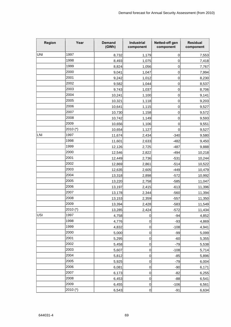
Demand forecast for Annual Security Assessment (from 2010)
644031-4 69
Region Year Demand (GWh)
Industrial component
Netted-off gen component
Residual component
UNI 1997 8,732 1,179 0 7,553
1998 8,493 1,075 0 7,418
1999 8,824 1,056 0 7,767
2000 9,041 1,047 0 7,994
2001 9,242 1,012 0 8,230
2002 9,582 1,044 0 8,537
2003 9,743 1,037 0 8,706
2004 10,241 1,100 0 9,141
2005 10,321 1,118 0 9,203
2006 10,641 1,115 0 9,527
2007 10,730 1,158 0 9,572
2008 10,742 1,149 0 9,593
2009 10,656 1,106 0 9,551
2010 (*) 10,654 1,127 0 9,527
LNI 1997 11,674 2,434 -340 9,580
1998 11,601 2,633 -482 9,450
1999 12,126 2,725 -487 9,888
2000 12,546 2,822 -494 10,218
2001 12,449 2,736 -531 10,244
2002 12,869 2,861 -514 10,522
2003 12,635 2,605 -449 10,479
2004 13,318 2,898 -572 10,992
2005 13,220 2,758 -585 11,047
2006 13,197 2,415 -613 11,396
2007 13,178 2,344 -560 11,394
2008 13,153 2,359 -557 11,350
2009 13,394 2,428 -583 11,549
2010 (*) 13,285 2,424 -572 11,434
USI 1997 4,758 0 -94 4,852
1998 4,776 0 -93 4,869
1999 4,832 0 -108 4,941
2000 5,000 0 -99 5,099
2001 5,295 0 -60 5,355
2002 5,458 0 -79 5,538
2003 5,607 0 -108 5,714
2004 5,812 0 -85 5,896
2005 5,925 0 -79 6,004
2006 6,081 0 -90 6,171
2007 6,173 0 -82 6,255
2008 6,453 0 -88 6,541
2009 6,455 0 -106 6,561
2010 (*) 6,543 0 -91 6,634

Demand forecast for Annual Security Assessment (from 2010)
70 644031-4
Region Year Demand (GWh)
Industrial component
Netted-off gen component
Residual component
LSI 1997 6,913 4,808 -174 2,279
1998 7,043 4,905 -180 2,318
1999 7,170 5,008 -168 2,330
2000 7,208 5,023 -197 2,383
2001 7,198 4,944 -193 2,447
2002 7,452 5,088 -176 2,540
2003 7,497 5,050 -168 2,615
2004 7,779 5,210 -141 2,710
2005 7,654 5,234 -212 2,632
2006 7,678 5,093 -149 2,734
2007 7,952 5,321 -184 2,815
2008 7,565 4,816 -149 2,898
2009 7,015 4,226 -146 2,935
2010 (*) 7,946 5,278 -198 2,866
(*) - Values for 2010 include some imputed data, since the 2010 year was not complete at time of writing
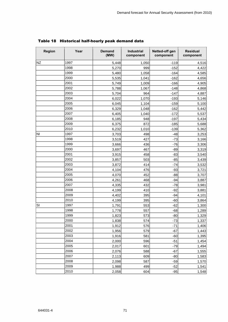
Demand forecast for Annual Security Assessment (from 2010)
644031-4 71
Table 18 Historical half-hourly peak demand data
Region Year Demand (MW)
Industrial component
Netted-off gen component
Residual component
NZ 1997 5,448 1,050 -119 4,516
1998 5,270 999 -152 4,422
1999 5,480 1,058 -164 4,585
2000 5,535 1,041 -162 4,656
2001 5,749 1,009 -166 4,905
2002 5,788 1,067 -148 4,868
2003 5,704 964 -147 4,887
2004 6,022 1,070 -193 5,146
2005 6,045 1,104 -159 5,100
2006 6,329 1,048 -162 5,442
2007 6,405 1,040 -172 5,537
2008 6,185 948 -197 5,434
2009 6,375 872 -185 5,688
2010 6,232 1,010 -139 5,362
NI 1997 3,703 498 -48 3,253
1998 3,519 427 -73 3,166
1999 3,666 436 -76 3,306
2000 3,697 467 -89 3,319
2001 3,915 458 -83 3,540
2002 3,857 503 -85 3,439
2003 3,872 414 -74 3,532
2004 4,104 476 -93 3,721
2005 4,070 452 -88 3,707
2006 4,261 468 -94 3,887
2007 4,335 432 -78 3,981
2008 4,199 410 -92 3,881
2009 4,402 395 -94 4,101
2010 4,199 395 -60 3,864
SI 1997 1,791 553 -62 1,300
1998 1,778 557 -68 1,289
1999 1,823 573 -80 1,329
2000 1,838 574 -73 1,337
2001 1,912 576 -71 1,406
2002 1,956 579 -67 1,443
2003 1,916 581 -60 1,395
2004 2,000 596 -51 1,454
2005 2,017 601 -79 1,494
2006 2,076 588 -67 1,555
2007 2,113 609 -80 1,583
2008 2,098 587 -59 1,570
2009 1,988 499 -52 1,541
2010 2,058 604 -95 1,548
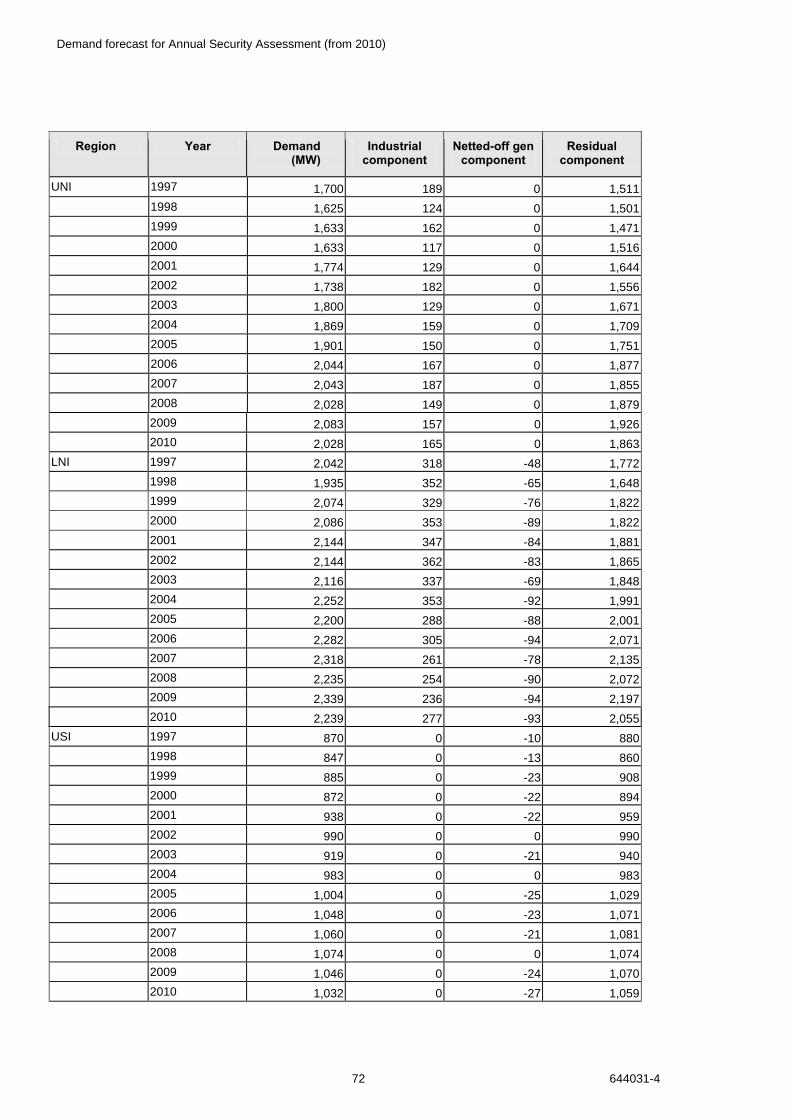
Demand forecast for Annual Security Assessment (from 2010)
72 644031-4
Region Year Demand (MW)
Industrial component
Netted-off gen component
Residual component
UNI 1997 1,700 189 0 1,511
1998 1,625 124 0 1,501
1999 1,633 162 0 1,471
2000 1,633 117 0 1,516
2001 1,774 129 0 1,644
2002 1,738 182 0 1,556
2003 1,800 129 0 1,671
2004 1,869 159 0 1,709
2005 1,901 150 0 1,751
2006 2,044 167 0 1,877
2007 2,043 187 0 1,855
2008 2,028 149 0 1,879
2009 2,083 157 0 1,926
2010 2,028 165 0 1,863
LNI 1997 2,042 318 -48 1,772
1998 1,935 352 -65 1,648
1999 2,074 329 -76 1,822
2000 2,086 353 -89 1,822
2001 2,144 347 -84 1,881
2002 2,144 362 -83 1,865
2003 2,116 337 -69 1,848
2004 2,252 353 -92 1,991
2005 2,200 288 -88 2,001
2006 2,282 305 -94 2,071
2007 2,318 261 -78 2,135
2008 2,235 254 -90 2,072
2009 2,339 236 -94 2,197
2010 2,239 277 -93 2,055
USI 1997 870 0 -10 880
1998 847 0 -13 860
1999 885 0 -23 908
2000 872 0 -22 894
2001 938 0 -22 959
2002 990 0 0 990
2003 919 0 -21 940
2004 983 0 0 983
2005 1,004 0 -25 1,029
2006 1,048 0 -23 1,071
2007 1,060 0 -21 1,081
2008 1,074 0 0 1,074
2009 1,046 0 -24 1,070
2010 1,032 0 -27 1,059

Demand forecast for Annual Security Assessment (from 2010)
644031-4 73
Region Year Demand (MW)
Industrial component
Netted-off gen component
Residual component
LSI 1997 936 553 -46 429
1998 944 564 -51 431
1999 949 573 -33 408
2000 969 574 -20 415
2001 990 576 -51 465
2002 1,000 579 -53 474
2003 996 581 -39 455
2004 1,023 596 -51 477
2005 1,030 599 -22 453
2006 1,036 588 -42 490
2007 1,061 609 -51 503
2008 1,046 595 0 451
2009 985 510 0 474
2010 1,054 611 -53 497
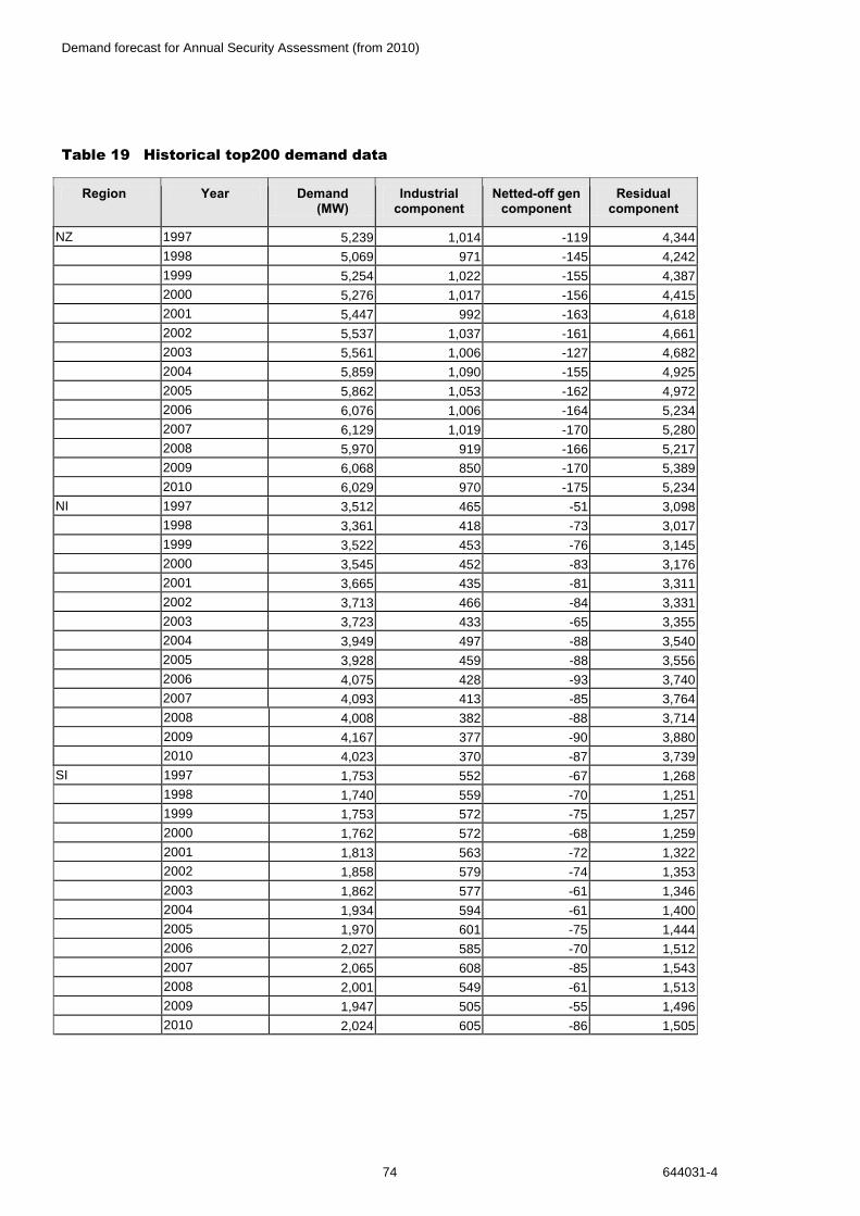
Demand forecast for Annual Security Assessment (from 2010)
74 644031-4
Table 19 Historical top200 demand data
Region Year Demand (MW)
Industrial component
Netted-off gen component
Residual component
NZ 1997 5,239 1,014 -119 4,344
1998 5,069 971 -145 4,242
1999 5,254 1,022 -155 4,387
2000 5,276 1,017 -156 4,415
2001 5,447 992 -163 4,618
2002 5,537 1,037 -161 4,661
2003 5,561 1,006 -127 4,682
2004 5,859 1,090 -155 4,925
2005 5,862 1,053 -162 4,972
2006 6,076 1,006 -164 5,234
2007 6,129 1,019 -170 5,280
2008 5,970 919 -166 5,217
2009 6,068 850 -170 5,389
2010 6,029 970 -175 5,234
NI 1997 3,512 465 -51 3,098
1998 3,361 418 -73 3,017
1999 3,522 453 -76 3,145
2000 3,545 452 -83 3,176
2001 3,665 435 -81 3,311
2002 3,713 466 -84 3,331
2003 3,723 433 -65 3,355
2004 3,949 497 -88 3,540
2005 3,928 459 -88 3,556
2006 4,075 428 -93 3,740
2007 4,093 413 -85 3,764
2008 4,008 382 -88 3,714
2009 4,167 377 -90 3,880
2010 4,023 370 -87 3,739
SI 1997 1,753 552 -67 1,268
1998 1,740 559 -70 1,251
1999 1,753 572 -75 1,257
2000 1,762 572 -68 1,259
2001 1,813 563 -72 1,322
2002 1,858 579 -74 1,353
2003 1,862 577 -61 1,346
2004 1,934 594 -61 1,400
2005 1,970 601 -75 1,444
2006 2,027 585 -70 1,512
2007 2,065 608 -85 1,543
2008 2,001 549 -61 1,513
2009 1,947 505 -55 1,496
2010 2,024 605 -86 1,505
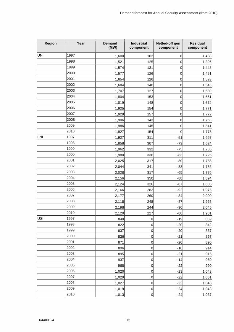
Demand forecast for Annual Security Assessment (from 2010)
644031-4 75
Region Year Demand (MW)
Industrial component
Netted-off gen component
Residual component
UNI 1997 1,600 162 0 1,438
1998 1,521 125 0 1,396
1999 1,574 131 0 1,443
2000 1,577 126 0 1,451
2001 1,654 126 0 1,528
2002 1,684 140 0 1,545
2003 1,707 127 0 1,580
2004 1,804 153 0 1,651
2005 1,819 148 0 1,672
2006 1,925 154 0 1,771
2007 1,929 157 0 1,772
2008 1,906 143 0 1,763
2009 1,986 145 0 1,841
2010 1,927 154 0 1,773
LNI 1997 1,927 311 -51 1,667
1998 1,858 307 -73 1,624
1999 1,962 332 -75 1,705
2000 1,980 336 -83 1,726
2001 2,025 317 -80 1,788
2002 2,044 341 -83 1,786
2003 2,028 317 -65 1,776
2004 2,156 350 -88 1,894
2005 2,124 326 -87 1,885
2006 2,166 282 -92 1,976
2007 2,177 260 -84 2,000
2008 2,118 248 -87 1,958
2009 2,198 244 -90 2,045
2010 2,120 227 -88 1,981
USI 1997 840 0 -19 859
1998 822 0 -20 842
1999 837 0 -20 857
2000 836 0 -21 857
2001 871 0 -20 890
2002 896 0 -18 914
2003 895 0 -21 916
2004 937 0 -14 950
2005 968 0 -22 990
2006 1,020 0 -23 1,043
2007 1,029 0 -22 1,051
2008 1,027 0 -22 1,048
2009 1,019 0 -24 1,043
2010 1,013 0 -24 1,037

Demand forecast for Annual Security Assessment (from 2010)
76 644031-4
Region Year Demand (MW)
Industrial component
Netted-off gen component
Residual component
LSI 1997 918 552 -46 413
1998 925 560 -47 413
1999 927 572 -39 394
2000 942 572 -33 403
2001 962 573 -48 438
2002 971 579 -51 444
2003 977 584 -33 426
2004 1,006 594 -39 451
2005 1,008 601 -51 458
2006 1,015 590 -44 470
2007 1,045 608 -56 493
2008 1,021 590 -11 442
2009 976 567 -9 418
2010 1,028 608 -45 466


