DEMAND FORECASTING IN TEXTILE INDUSTRY- A CASE STUDY

DEMAND FORECASTING IN TEXTILE INDUSTRY- A CASE STUDY

By

MUHAMMAD OBYDULL AKBAR

A Thesis Submitted to the

Department of Industrial and Production Engineering,

Bangladesh University of Engineering & Technology

In Partial Fulfillment of the requirements for the Degree of

MASTER OF ENGINEERING IN ADVANCED ENGINEERING MANAGEMENT

DEPARTMENT OF INDUSTRIAL AND PRODUCTION ENGINEERING (IPE)

BANGLADESH UNIVERSITY OF ENGINEERING AND TECHNOLOGY (BUET)

Dhaka, Bangladesh

November, 2013

i

DEMAND FORECASTING IN TEXTILE INDUSTRY- A CASE STUDY

By

MUHAMMAD OBYDULL AKBAR

A Thesis Submitted to the

Department of Industrial and Production Engineering,

Bangladesh University of Engineering & Technology

In Partial Fulfillment of the requirements for the Degree of

MASTER OF ENGINEERING IN ADVANCED ENGINEERING MANAGEMENT

DEPARTMENT OF INDUSTRIAL AND PRODUCTION ENGINEERING (IPE)

BANGLADESH UNIVERSITY OF ENGINEERING AND TECHNOLOGY (BUET)

Dhaka, Bangladesh

November, 2013

ii

CERTIFICATE OF APPROVAL

The thesis titled ―Demand Forecasting in Textile Industry-A case study‖ submitted by

Muhammad Obydull Akbar, Student No. 0411082147, Session- April 2011, has been

accepted as satisfactory in partial fulfillment of the requirements for the degree of Master of

Engineering in Advanced Engineering Management on 30th November, 2013.

BOARD OF EXAMINERS

Dr. M, Ahsan Akhtar Hasin

Professor

Department of Industrial & Production Engineering

BUET, Dhaka

Chairman

(Supervisor)

Dr. Abdullahil Azeem

Professor


BUET, Dhaka

Member

Dr. Sultana Parveen

Professor & Head


BUET, Dhaka

Member

iii

CANDIDATE’S DECLARATION

It is hereby declared that this thesis or any part of it has not been submitted elsewhere for the

award of any degree or diploma.

Muhammad Obydull Akbar

iv

This Work is dedicated to My Parents

& My Family

v

ACKNOWLEDGEMENT

At first, the author wants to convey his deepest gratefulness to the almighty God, the

beneficial, the merciful for granting me to bring this research work into light. This author

would like to express his sincere respect and gratitude to honorable teacher & thesis

supervisor, Dr. M, Ahsan Akhtar Hasin, Professor, Department of Industrial and production

Engineering(IPE), Bangladesh University of Engineering and Technology(BUET), Dhaka,

for his thoughtful suggestions, constant guidance and encouragement throughout the progress

of this research work. The author also expressed his sincere gratitude to Dr. Md. Abdillahil Azeem, Professor,

Department of Industrial and production Engineering (IPE), BUET, Dr. Sultana Parveen,

Professor & Head, Department of Industrial and production Engineering (IPE), BUET for

their constructive remarks & for kindly evaluating this research.

The author is especially thankful to Mr. G.M. Salahuddin, Manager, Supply Chain

department, Epyllion Group, for his cordial encouragement & sincere help during the data

collection phase and permitting me to have accessed to his company.

Moreover the author also thankful to all the personnel of CMA team, IE team, manager of IE

team, quality inspectors etc.

The author is grateful to all the writers and publishers of the books and journal papers that

have taken as references while conducting this research.

With a very special recognition, the author would like to thanks his parents as well as all the

members of his families, who provided their continuous inspirations, sacrifice and support

encouraged me to complete the research work successfully.

vi

ABSTRACT

Forecasts are usually made to help and guide decision making. Good forecasts are

preconditions for good, informed decisions. These decisions may vary from a financial

market bet on interest rate changes to the policy decision on how to structure a country's

pension system. Ideally, decision-makers should be as well prepared as possible for the

future, which would allow them to act appropriately. To detect challenges and opportunities

in a timely manner decision-makers require a good forecasting framework. Given the role

governments, companies and individuals play, knowledge about the drivers and linkages that

determine the future will allow these players to actually shape the future themselves.

Decision makers need forecasts only if there is uncertainty about the future. Thus, we have no

need to forecast whether the sun will rise tomorrow. There is also no uncertainty when events

can be controlled. Many decisions, however, involve uncertainty, and in these cases, formal

forecasting procedures can be useful. There are alternatives to forecasting. A decision maker

can buy insurance, hedge, or use ―just-in-time‖ systems. Another possibility is to be flexible

about decisions. Forecasting is often confused with planning. Planning concerns what the

world should look like, while forecasting is about what it will look like. Planners can use

forecasting methods to predict the outcomes for alternative plans. If the forecasted outcomes

are not satisfactory, they can revise the plans, and then obtain new forecasts, repeating the

process until the forecasted outcomes are satisfactory. They can then implement and monitor

the actual outcomes to use in planning the next period.

This process might seem obvious. However, in practice, many organizations revise their

forecasts, not their plans. They believe that changing the forecasts will change behavior.

Forecasting serves many needs. It can help people and organizations to plan for the future and

to make rational decisions. It can help in deliberations about policy variables.

vii

TABLE OF CONTENTS

Acknowledgement …………………...v

Abstract …………………...vi

Table of Contents …………………...vii

Chapter 1 Introduction ……………………...1

1.1 Background ……………………...1

1.2 Rationale of the study ……………………...3

1.3 Objectives of the study ……………………...3

1.4 Outline of methodology ……………………...4

Chapter 2 Literature Review ……………………...5

2.1 Forecasting ……………………...5

2.2 Hypothesis Testing ...…………………..23

2.2.1 Sampling Plan …………………..32

Chapter 3 Theoretical Framework …………………...35

3.1 Forecasting evaluations …………………...35

3.1.1 Grass Roots …………………...35

3.1.2 Market Research …………………...35

3.1.3. Panel Consensus …………………...36

3.1.4 Delphi Method …………………...36

3.1.5 Time Series Analysis …………………...37

3.1.6 Forecast Errors …………………....38

3.1.7 Sources of Error …………………...38

3.1.8 Components of demand …………………...39

3.1.9Additive Seasonal Variation …………………...40

3.1.10 Multiplicative Seasonal

Variation

…………………...40

3.1.11 Seasonal Factor (or Index) …………………...40

3.2 Weighted Moving Average …………………...40

3.2.1 Choosing Weights …………………...40

3.3 Exponential Smoothing …………………....41

3.4 Linear Regression Analysis …………………....41

3.5 Least Squares Method …………………...42

viii

3.5.1 Choosing appropriate

value for alpha

…………………....44

3.6 Statistical Quality Control …………………...44

3.7 Acceptance Sampling …………………...46

3.7.1 Consider Process Stability …………………...47

3.7.2 Consider Lot Size …………………...48

3.7.3 Errors in control chart …………………...49

3.7.4 P-value Decision Criterion …………………...50

Chapter 4 Problem Analysis …………………...50

4.1 Naïve Approach …………………...50

4.2 Simple Moving Average …………………...53

4.3 Weighted Moving Average …………………...57

4.4 Exponential Smoothing …………………...59

4.5 Seasonal Index

…………………...61

Chapter 5 Statistical Analysis …………………...64

5.1 Statistical Analysis …………………...64

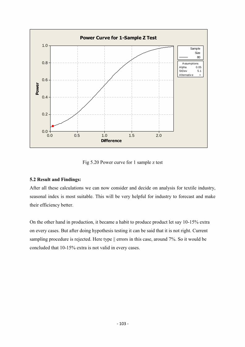
5.2 Result and Findings …………………...103

Chapter 6 Conclusions & Recommendations …………………...104

6.1 Conclusions …………………...104

6.2 Recommendations …………………...106

References …………………...106

Appendices …………………...109

- 1 -

CHAPTER 1

INTRODUCTION

1.1 Background

Forecasting is estimate of the occurrence, timing of magnitude of uncertain future events. It is

also a measure of uncertainty of market demand in case of a business organization. It is the

basis of all subsequent planning activities of a production industry. Thus it is essential for

smooth operations of all business activities. They provide information that can assist

managers in guiding future activities toward organizational goals. Either operations

department or planning department or even marketing is seen performing this vital task.

Procurement of raw materials, logistical arrangements, and warehouse arrangements largely

depends on this. It in fact affects the operations of the whole supply chain [1].

In an industrial environment, forecasts of demand are based primarily on non-random trends

and relationships, with an allowance for random components [2]. Forecasts for group of

products, as is the usual case in a textile production industry, tend to be more accurate than

those for single products.

Textile industry is the leading industrial sector in Bangladesh. A composite textile company,

being partially vertically integrated, performs business operations of many stages of the long

supply chain. It requires different types if raw materials in different forms, where output of

one section provides input to other section. In case of woven type Ready-Made

Garments(RMG), generally only one step of operations are done, where input raw materials

are different for different jobs, requiring order-specific raw materials acquisition. Thus

importance of forecast of input materials becomes less significant. However the knit sector of

textile industry is less import oriented than woven sector. The composite knit industry

produced a large portion of input materials locally in the same industry, acting as feeders of

the knit RMG factory. Thus forecast of raw materials, not essentially the cloth is of more

importance [3].

For a complete supply chain to be successful, accurate forecasting has no alternative.

Experiences in different countries reveal that for consumer goods, such as apparel products,

- 2 -

variation in demand creates frequent out of stock, which ultimately leads to customer

dissatisfaction [4, 5].

Forecasts are vital to every business organization and for every significant management

decision. While a forecast is never perfect due to the dynamic nature of the external business

environment, it is beneficial for all levels of functional planning, strategic planning, and

budgetary planning.

Decision-makers use forecasts to make many important decisions regarding the future direction of the organization.

Demand forecasting includes the prediction, projection or estimation of expected demand of

the products over a specified future time period. The demand of seasonal products frequently

changes in the marketplace. As soon as the main selling season passes, the excessive

inventories of the product are devalued greatly. On the other hand, if the product supplies

were relatively short, a direct sale loss occurs. Therefore, demand planning is considered the

first step of a supply chain planning process, which provides a continuous link to manage the

inventory position and the product demand.

Demand management exists to coordinate and control all sources of demand so the

productive system can be used efficiently and the product delivered on time. Demand can be

either dependent on the demand for other products or services or independent because it

cannot be derived directly from that of other products.

Epyllion Group is one of the leading composite textile companies in Bangladesh. It is mainly

a composite textile company, engaged in manufacturing and exporting of knit apparels since

1994. The inventory record shows that high level of inaccuracy results in a huge loss in

inventory cost. This additionally adds to sales price of the knit products. This it is very

essential for them to forecast the demand of various raw materials with higher level of

accuracy.

This research project aims at providing information about future trend of apparel demand,

create forecast using necessary tools and find out extra production and their relevance.

- 3 -

1.2 Rationale of the study Forecasts are vital to every business organization and for every significant management

decision. Forecasting is the basis of corporate long-run planning. In the functional areas of

finance and accounting, forecasts provide the basis for budgetary planning and cost control.

Marketing relies on sales forecasting to plan new products, compensate sales personnel, and

make other key decisions. Production and operations personnel use forecast to make periodic

decisions involving process selection, capacity planning, and facility layout, as well as for

continual decisions about production planning, scheduling and inventory.

Bear in mind that a perfect forecast is usually impossible. Too many factors in the business

environment cannot be predicted with certainty. Therefore, rather than search for the perfect

forecast, it is far more important to establish the practice of continual review of forecasts and

to learn to live with inaccurate forecasts. This is not to say that we should not try to improve

the forecasting model or methodology, but that we should try to find and use the best

forecasting method available, within reason. Forecasting is an essential tool for making

strategic demand planning. In this study, a number of demand forecasting models are studied

to predict demand of a seasonal product for an active sales period. Forecasting accuracy may

be measured using several indicators, such as relative error, mean absolute deviation and

tracking signals. After forecasts are derived, the inventory quantity for a target business

season can be obtained based on these demand forecasts.

1.3 Objectives of the study

The specific objectives of this research work as follows:

1. Identify the pattern of demand of apparel products, factors affecting the pattern and

their degree of relevance.

2. Deseasonalize the demand pattern.

3. Estimate the demand by using linear regression analysis.

4. Control chart analysis on sample testing

5. Suggestion based on analysis rather than average production.

- 4 -

1.4 Outline of methodology

The following step by step methodology has been applied to this research project:

a. Study marketing and sales pattern of different types of apparel products.

b. Identify the factors affecting the demand.

c. Identify seasonal impact on the demand pattern.

d. Deseasonalize the seasonal impact.

e. Analyze correlation for the related factors.

f. Apply different methods of forecasting such as, linear regression analysis, weighted

moving average, Exponential smoothing, and naïve approach to estimate demands.

g. Doing all the analysis on Microsoft Excel due to availability of this software in every

factory of our country.

h. Find out the errors- Mean absolute deviation (MAD), Mean squared error (MSD),

Mean absolute percent error (MAPE) of these forecasting methods.

i. Suggest a forecasting model, appropriate for seasonal apparel products.

j. Control chart analysis on sample testing.

k. Make hypothesis to reject the sample test

l. Finding type I error and type II error

m. Refuse average production on 10-15% extra in every order and make suggestion basis

on analysis.

- 5 -

CHAPTER 2

LITERATURE REVIEW

2.1 Forecasting

Forecasting techniques can be categorized in two broad categories: quantitative and

qualitative. The techniques in the quantitative category include mathematical models such as

moving average, straight-line projection, exponential smoothing, regression, trend-line

analysis, simulation, life-cycle analysis, decomposition, Box-Jenkins, expert systems, and

neural network. The techniques in the qualitative category include subjective or intuitive

models such as jury or executive opinion, sales force composite, and customer expectations

[6].

Along with qualitative and quantitative, forecasting models can be categorized as time-series,

causal, and judgmental. A time-series model uses past data as the basis for estimating future

results. The models that fall into this category include decomposition, moving average,

exponential smoothing, and Box-Jenkins. The premise of a causal model is that a particular

outcome is directly influenced by some other predictable factor.

These techniques include regression models. Judgmental techniques are often called

subjective because they rely on intuition, opinions, and probability to derive the forecast.

These techniques include expert opinion, Delphi, sales force composite, customer

expectations (customer surveys), and simulation. [7]

Typically, the two forms of forecasting error measures used to judge forecasting performance

are mean absolute deviation (MAD) and mean absolute percentage error (MAPE). For both

MAD and MAPE, a lower absolute value is preferred to a higher absolute value. MAD is the

difference between the actual sales and the forecast sales, absolute values are calculated over

a period of time, and the mean is derived from these absolute differences. MAPE is used

with large amounts of data, and forecasters may prefer to measure error in percentage

- 6 -

Three planning horizons for forecasting exist. The short-term forecast usually covers a

period of less than three months. The medium-term forecast usually covers a period of three

months to two years. And, the long-term forecast usually covers a period of more than two

years. Generally, the short-term forecast is used for the daily operation and plans of a

company. The long-term forecast is used more for strategic planning.

According to Makridakis forecasting is needed since there usually is a time lag between

upcoming need and the time the need occurs, this time lag is called lead time. Forecasts are

created to predict future needs and these predictions are then used to help in effective

and efficient planning . This section will explain some general factors of forecasting [8].

Authors considered methods for forecasting brand sales utilizing wavelet decompositions of

related causal series. Wavelet decompositions can uncover the hidden periodicities inherent

in marketing time series like pricing and can therefore provide superior information in causal

sales forecasting methods. The paper specifically addressed the problem of multi co linearity

since the proposed wavelet packet transformation of a time series of length T generates 2T –

2 correlated vectors of coefficients, each of length T. It was found that partial least-squares

provide the most accurate forecasting method which at the same time achieves the desired

dimension reduction in the estimation problem.

In trying to forecast demand for a new product, as ideal situation would be where an existing

product or generic product could be used as a model. There are many ways to classify such

analogies-for example, complementary products, substitutable or competitive products and

product as a function of income. A casual relationship would be that demand for compact

discs is caused by demand for CD players. An analogy would be forecasting the demand for

digital video disk players by analyzing the historic demand for stereo VCRs. The products are

in the same general category of electronics and may be bought by consumers at similar rates.

A similar example would be toasters and coffee pots. A firm that already produces toasters

and wants to produce coffee pots could use the toaster as a likely growth model.

This study aims to test on the predictability of Credit Hire services for the automobile and

insurance industry. A relatively sophisticated time series forecasting procedure, which

conducts a competition among exponential smoothing models, is employed to forecast

- 7 -

demand for a leading UK Credit Hire operator (CHO). The generated forecasts are compared

against the Naive method, resulting that demand for CHO services is indeed extremely hard

to forecast, as the underlying variable is the number of road accidents – a truly stochastic

variable.

Promotions are an integral part of the consumer packaged goods (CPG) industry. Anywhere

between 30-40% of the sales volumes are achieved through various promotions. Promotions

are instrumental in creating brand visibility and awareness. In this study, we attempt to

analyze the impact of promotions with feature advertises, in-store display, temporary price

discounts etc. Five different multivariate regression models have been developed to forecast

the total sales of a product considering pricing and distribution variables. The performance of

these models has been analyzed by using syndicated data. Based on the results, it is found

that the S-shaped (double-log) model has shown superior performance over the other models

considered in this study.

Customer-driven orientation for continuous improvement is an essential element embedded in

the service industry. Sales representatives stress the unique qualities of their products or

services to emulate and improve upon existing and potential competitors resulted in making

their customers satisfied and enhance the retention of valuable customers. This study employs

the five-dimensional structure of SERVQUAL as the decision service criteria by conducting

an interview with analysts from consumers' foundation, Chinese Taipei (CFCT) to evaluate

the service quality of 3C (computer, communication and consumer electronics) wholesalers

in Taiwan. This study intends to select a best practice for service as a benchmark through

which firms and their sales representatives can learn to increase workforce productivity and

improve sales performance. Fuzzy VIKOR method is utilized as systematic solution to solve

the complicated decision problems. The result shows that Fuzzy VIKOR provides an efficient

way to obtain a best and compromise solution for decision-making.

For a small retail distribution chain, demand forecasting is the main driver to effectiveness

and efficiency of a supply chain. However, as large number of varied models and products

are marketed through a super market, several attributes affect forecasting. Because of these

affecting parameters, nonlinearity arises. As a result, traditional forecasting approaches

cannot provide good estimation of demand. A fuzzy neural network analysis can provide

better solution in this case. This research first analyzed the trend and seasonality patterns of a

- 8 -

selected product in a retail distribution chain in Bangladesh. Then demand was forecasted

using traditional Holt-Winter’s model. The same was done again using artificial neural

network (ANN) with fuzzy uncertainty. Finally, the errors, measured in terms of MAPE,

were compared for finding the best fitting forecasting approach. The research found that the

error levels in Holt-Winter’s approach are higher than those obtained through fuzzy ANN

approach. This is because of influence of several factors on demand function in retail

distribution system. It was also observed that as forecasting period becomes smaller, the

ANN approach provides more accuracy in forecast.

This project work investigates the role of cross-sectional dependence among private

forecasters, assessing its impact on the measurement and use of the forecasting uncertainty.

We determine the circumstances under which cross-sectional measures of uncertainty (such

as the disagreement across forecasters) are valid proxies for private information, and analyze

the impact of distributional assumptions on private signals. In particular, we explore the role

played by cross dependence among forecasters, arising from factors such as partially shared

private information. We validate the theory through a Monte Carlo exercise, which reinforces

our findings, as well as through an application to US nonfarm payroll data [8].

Forecasting researchers, with few exceptions, have ignored the current major forecasting

controversy: global warming and the role of climate modeling in resolving this challenging

topic. In this paper, we take a forecaster’s perspective in reviewing established principles for

validating the atmospheric-ocean general circulation models (AOGCMs) used in most

climate forecasting, and in particular by the Intergovernmental Panel on Climate Change

(IPCC). Such models should reproduce the behaviors characterizing key model outputs, such

as global and regional temperature changes. We develop various time series models and

compare them with forecasts based on one well-established AOGCM from the UK Hadley

Centre. Time series models perform strongly, and structural deficiencies in the AOGCM

forecasts are identified using encompassing tests. Regional forecasts from various GCMs had

even more deficiencies. We conclude that combining standard time series methods with the

structure of AOGCMs may result in a higher forecasting accuracy. The methodology

described here has implications for improving AOGCMs and for the effectiveness of

environmental control policies which are focused on carbon dioxide emissions alone.

Critically, the forecast accuracy in decadal prediction has important consequences for

- 9 -

environmental planning, so its improvement through this multiple modeling approach should

be a priority.

Despite the state of flux in media today, television remains the dominant player globally for

advertising spending. Since television advertising time is purchased on the basis of projected

future ratings, and ad costs have skyrocketed, there is increasingly pressure to forecast

television ratings accurately. The forecasting methods that have been used in the past are not

generally very reliable, and many have not been validated; also, even more distressingly,

none have been tested in today’s multichannel environment. In this study we compare eight

different forecasting models, ranging from a naïve empirical method to a state-of-the-art

Bayesian model-averaging method. Our data come from a recent time period, namely 2004–

2008, in a market with over 70 channels, making the data more typical of today’s viewing

environment. The simple models that are commonly used in industry do not forecast as well

as any econometric models. Furthermore, time series methods are not applicable, as many

programs are broadcast only once. However, we find that a relatively straightforward random

effects regression model often performs as well as more sophisticated Bayesian models in

out-of-sample forecasting. Finally, we demonstrate that making improvements in ratings

forecasts could save the television industry between $250 and $586 million per year.

This special section aims to demonstrate the limited predictability and high level of

uncertainty in practically all important areas of our lives, and the implications of this. It

summarizes the huge body of solid empirical evidence accumulated over the past several

decades that proves the disastrous consequences of inaccurate forecasts in areas ranging from

the economy and business to floods and medicine. The big problem is, however, that the great

majority of people, decision and policy makers alike still believe not only that accurate

forecasting is possible, but also that uncertainty can be reliably assessed. Reality, however,

shows otherwise, as this special section proves. This paper discusses forecasting accuracy and

uncertainty, and distinguishes three distinct types of predictions: those relying on patterns for

forecasting, those utilizing relationships as their basis, and those for which human judgment

is the major determinant of the forecast. In addition, the major problems and challenges

facing forecasters and the reasons why uncertainty cannot be assessed reliably are discussed

using four large data sets. There is also a summary of the eleven papers included in this

special section, as well as some concluding remarks emphasizing the need to be rational and

realistic about our expectations and avoid the common delusions related to forecasting.

- 10 -

Forecasts are crucial for practically all economic and business decisions. However, there is a

mounting body of empirical evidence showing that accurate forecasting in the economic and

business world is usually not possible. In addition, there is huge uncertainty, as practically all

economic and business activities are subject to events we are unable to predict. The fact that

forecasts can be inaccurate creates a serious dilemma for decision and policy makers. On the

one hand, accepting the limits of forecasting accuracy implies being unable to assess the

correctness of decisions and the surrounding uncertainty. On the other hand, believing that

accurate forecasts are possible means succumbing to the illusion of control and experiencing

surprises, often with negative consequences. We believe that the time has come for a new

attitude towards dealing with the future. In this article, we discuss the limited predictability in

the economic and business environment. We also provide a framework that allows decision

and policy makers to face the future — despite the inherent limitations of forecasting and the

uncertainty, sometimes huge, surrounding most future-oriented decisions.

Makridakis explain that the need and interest for forecasting has been increasing since

company management aims to decrease the dependence on chance while trying to analyze the

environmental factors more scientifically. Management attitudes are changing but that is not

the only factor increasing the significance of forecasting. The changes in the business

environment and consumer behavior have caused forecasting to become a critical

operational function, he clarifies that the changes in the business environment have

caused companies to rely more on forecasting to be able to meet the market needs better.

Over the year’s business environment has changed from push to pull manufacturing.

This change from push to pull manufacturing means that instead of producing goods

prior to customer need, now companies are using customer demand as the factor

which initiates production explains that during this manufacturing style change also market

power has shifted from manufacturers towards retailers and consumers. Also other changes

in the business environment such as increased competition and shorter product

development cycles have increased the need for forecasting schemes [9].

All these changes have increased the significance of forecasting but these have also been

detrimental to forecast accuracy and costs related to forecasting errors have increased. For

this reason, further research is needed to examine how to increase forecast accuracy

while maintaining the costs low.

- 11 -

Forecasting practices in organizations vary due to different planning needs and product

types. According to Arnold forecasting has few basic characteristics which are very simple

and understanding them will make forecasting easier and enable more effective goods

prior to customer need, now companies are using customer demand as the factor

which usage of the forecasts. Understanding the forecasting basics provides awareness to

the forecast planners about the challenges of forecasting. These four characteristics are listed

and explained below [10].

Finally, the distinction between the forecasting method and forecasting system is important.

A forecasting method is a mathematical or subjective technique that forecasts some future

value or event. While many statistical forecasting software packages are implementations of

forecasting methods, they are not forecasting systems. A forecasting system is a computer-

based system that collects and processes demand data for thousands of items, develops

forecasts using forecasting methods, has an interactive management- user interface, maintains

a database of demands, and has report file-writing capabilities.

A forecasting system is much more complex than a forecasting method. The method is a part

of the system.

Demand forecasting is a challenging task since multiple factors need to be considered before

a forecasting process can be established and after the process has been created, continuous

monitoring is a key factor in improving the accuracy of the forecasts. When forecasting

activities are executed and monitored correctly, companies are able to be more efficient and

more profitable. If forecasts are created but not monitored, significant monetary losses or

even bankruptcy might occur. Especially when economic conditions are uncertain, it is

important for companies to cut costs in the supply chain and creating accurate forecast is one

way to accomplish this. All these issues related to forecasting emphasize the fact that demand

forecasting and especially NPF is a task which needs time, attention, and dedication in order

to provide the best possible results.

The subjects of new product development (NPD) and forecasting demand for ongoing

products have been quite widely covered topic in literature however the number of

publications available about new product forecasting (NPF) is considerably less. It also seems

that majority of the literature regarding NPF concentrates on the 3 forecasting techniques and

- 12 -

not on management issues. NPF is an intriguing and challenging research topic which can be

studied from many perspectives and it is definitely a topic which needs more research.

All the reasons above indicate that NPF is a complex but also very intriguing research

subject.

The motivation of this thesis is to investigate NPF recommendations and to gather insights

about NPF practices and forecasting challenges in Finnish textile companies. Two common

reasons why many companies struggle with NPF are due to its characteristics of low

creditability and low accuracy rates. The aim of this thesis is to discover which issues should

be considered and what actions should be taken to be able to create quality forecasts for new

products. Quality forecasts should be both accurate and creditable. Literature review section

will provide information and insights about forecasting best practices gathered from variety

of publications and journal articles written by experts to guide the analysis in the empirical

section [11].

The empirical section will explain forecasting practices in the selected companies and discuss

the findings of the literature review and empirical research.

Uncertainty fuels the need for risk management although risk, if adequately measured, may

be less than uncertainty, if measurable. Forecasting may be viewed as a bridge between

uncertainty and risk if a forecast peels away some degrees of uncertainty but on the other

hand, for example, may increase the risk of inventory. Therefore, forecasting continues to

present significant challenges. Presented findings from electronics industry, where original

equipment manufacturers (OEM) could not predict demand beyond a 4 week horizon. Moon

et al (1998) presented demand forecasting from Lucent (Alcatel-Lucent), demonstrating

improvement in forecasting accuracy (60% to 80-85%). Related observations resulted in

inventory mark downs [12].

Availability of increasing volumes of data demands tools that can extract value from data.

Recent research has shown that advanced forecasting tools enable improvements in supply

chain performance if certain pre-requisites are optimized (ordering policies, inventory

collaboration). Autoregressive models have been effective in macroeconomic inventory

forecasts and emphasize that the role of forecasting in supply chain is to indicate the right

direction for the actors rather than being exactly right, at every moment. Choosing the correct

forecasting method is often a complex issue.

- 13 -

It is often important to forecast the reactions of suppliers, distributors, and government in

order to develop a successful marketing strategy. On occasion, one might also need to

forecast the actions of other interest groups, such as ―concerned minorities.‖ A range of

techniques similar to those for forecasting competitors’ actions appears useful, but little

research investigates the relative accuracy of these techniques.

As with forecasting competitors’ actions, different techniques may suit different situations.

In an attempt to forecast the decisions by supermarkets, Montgomery developed a model of a

supermarket buying committee. Predictions were made about the shelving of a new product.

The model, based on information such as advertising for the product, reputation of the

supplier, margin, product novelty, and retail price, provided reasonable predictions for a hold-

out sample.

In Armstrong, role playing was used to forecast relations between suppliers and distributors.

In the role play, Philco (called Ace Company in the role play), a producer of home

appliances, was trying to improve its share of a depressed market. Philco had developed a

plan to sell appliances in supermarkets using a cash register tape discount plan. Secrecy was

important because Philco wanted to be first to use this strategy.

Implementation of such a plan depended upon the supermarket managers. Would the plan be

acceptable to them? In this case, a simple role playing procedure produced substantially more

accurate forecasts of the supermarket managers’ responses (8 of 10 groups were correct) than

did unaided opinions (1 of 34 groups was correct). In the actual situation, the supermarket

managers did accept the plan proposed by Philco.

(Incidentally, the change in distribution channels led to substantial losses for Philco.) The

superior accuracy of role playing relative to opinions seems to be due to its ability to provide

a more realistic portrayal of the interactions.

New product introductions have become a crucial part of survival for many businesses. One

of the reasons for the frequent product introductions is that product life cycles have become

shorter; therefore a way to stay ahead in today’s market is to continuously introduce new

products .In the recent years also the business environment has changed. Jain states that new

product development (NPD) is not an option anymore it has become a necessity. A fact of

today’s business environment is that introducing new products and/or services have become

vital for companies long-term growth (Fisher 1997; Simon 2010). Modern time series

- 14 -

forecasting methods are essentially rooted in the idea that the past tells us something about

the future. Of course, the question of how exactly we are to go about interpreting the

information encoded in past events, and furthermore, how we are to extrapolate future events

based on this information, constitute the main subject matter of time series analysis [13].

Typically, the approach to forecasting time series is to first specify a model, although this

need not be so. This model is a statistical formulation of the dynamic relationships between

that which we observe (i.e. the so called information set), and those variables we believe are

related to that which we observe. It should thus be stated immediately that this discussion will

be restricted in scope to those models which can formulated parametrically.

The ―classical‖ approach to time series forecasting derives from regression analysis. The

standard regression model involves specifying a linear parametric relationship between a set

of explanatory variables (or exogenous variables) and the dependent (or endogenous

variable). The parameters of the model can be estimated in a variety of ways, going back as

far as Gauss in 1794 with the ―Least Squares‖ method, but the approach always culminates in

striving for some form of statistical orthogonality between the explanatory variables and the

residuals (or innovations) of the regression. That is, we wish to express the linear relationship

in a dichotomous form in which the innovations represent that part of our information which

is completely unpredictable. It should probably also be emphasized that in the engineering

context this is analogous to reducing a signal to ―white noise.‖

However, this review is to be concerned with more ―modern‖ approaches and in many ways,

it was the practical necessities of engineering that provided an initial impetus. Both Wiener

(1949) and Kolmogorov (1941) were pioneers in the field of linear prediction, and while their

approaches differed (Wiener worked in the frequency domain popular amongst engineers,

while Kolmogorov worked in the time domain), it is clear that their solutions to the same

basic geometrical problem were equivalent.

Wiener’s work, in particular, was especially relevant to modern time series forecasting in that

he was among the first to rigorously formulate the problem of ―signal extraction.‖ That is,

given observations on a time series corrupted by additive noise, what is the optimal estimator

(in the mean-squared error (MSE) sense) of the latent or underlying signal (or state variable).

- 15 -

Given the historical context of massive systems of equations models popular among Macro

econometric forecasters of 1950’s or Adelmans it quickly became apparent that forecasting

models derived from a signal extraction context forecasted at least as well as those based on

complicated systems of economic relationship equations formulated as individual, yet

interconnected, dynamic classical regressions.

In most forecasting problems elegant mathematical models such as regression analysis,

weighted moving average or exponential smoothing models were developed in which the

forecasts are performed either by extrapolation or by averaging demand from the past data. In

these historical data-driven forecasting models, forecasts often exhibit the demand trend of

the past periods. Besides, the mathematical forecasting models do not permit integrating the

subjective information or experts’ views about the future demand in the forecasting

algorithm. They perform badly if the data series contains mission values. Therefore, forecasts

derived by past-data driven models may lead to a wrong conclusion about the future demand.

The demand of seasonal products varies from season to season, from one business cycle to

the next. In time series forecasting techniques such as autoregressive models, the parameters

of the models are always static. The static coefficient of a time series model cannot capture

the uncertainty of the future demand. The imposition of static models implies a fixed

relationship between the demand of the past season and the future. This may be considered

the inflexibility of the time series forecasting models.

The forecast of seasonal demand is essential for inventory planning prior to an active selling

season. In demand forecasting, a single model may not be adequate to represent a particular

demand series for all times. Further, the chosen model may have been restricted to a certain

class of time series. Therefore, a number of forecasting models are studied to provide wider

choices to find the best demand forecast of a seasonal product.

Davidson reported that one third of forecasters had worked as market research analysts before

becoming forecasters or forecast administrators and another third had held positions such as

field sales representative, budget analyst, data processing systems analyst, actuary or

consultant. A marketing background was also most frequently mentioned in the Cerullo and

Avila survey. Mentzer and Cox and Cerullo and Avila asked in their surveys how fore-

casters were trained. It seems that college courses and forecasting seminars are not a 'must'

for forecast preparers in companies, with only half of Mentzer and Cox's sample having

- 16 -

received formal training .On the other hand, Davidson reported that his sample of fore-casters

regarded college courses in "quantitative methods, computer literacy,

production/management, statistics, forecasting and market research" as "most important".

Surveys that focused on forecasting courses offered at universities agreed that business

schools emphasize different techniques (more quantitative than qualitative) than those

commonly used in the business world. Furthermore, training in data collection, monitoring

and evaluation of forecasts seemed to be rather neglected and a cause for concern given that

"the intended audience of most forecasting courses is future managers/decision makers and

not forecasters", and managers/decision makers are likely to spend a considerable time on

such activities .It stated that lack of formal training is often overrated, in that "the emphasis

should not be on increasing the forecaster's knowledge of sophisticated methods, since doing

so does not necessarily lead to improved performance. Perhaps the training should consider

such issues as how to select a time horizon, how to choose the length of a time period, how

judgment can be incorporated into a quantitative forecast, how large changes in the

environment can be monitored, and the level of aggregation to be forecast". Forecasting

managers in service firms appear, overall, to have a lower education level than their

counterparts in manufacturing companies while forecast preparers with graduate level

education are likely to employ more sophisticated techniques than their colleagues without

graduate education .Despite the high level of education found among forecasters in

manufacturing firms and the proposed positive correlation between education level and use of

more sophisticated forecasting techniques .forecast preparers in Sparkes and McHugh's

sample of manufacturing firms claimed to have the highest level of working knowledge in

subjective techniques such as executive assessment and surveys; one out of two respondents

declared only an "awareness", but no working knowledge, of exponential smoothing,

regression and correlation. The authors concluded that "the perceived 'complexity' of the

technique has a direct influence on the state of awareness and ultimate working knowledge of

formal techniques".

Several empirical studies focused on why businesses produce forecasts and the use they make

of the latter. In White's survey, 64% of respondents regarded the purpose of a sales forecast

as a goal setting device-a statement of desired performance; only 30% wanted to derive a true

assessment of the market potential. This finding was independent of firm size. However,

smaller firms used sales forecasts more often for personnel planning while for larger firms

sales quota setting and purchasing planning were frequent uses. Mentzer and Cox enquired

- 17 -

about the first, second and third most important areas of forecast usage. The majority of firms

regarded production planning and budgeting as important decision areas, a finding also

observed by Rothe (1978), McHugh and Sparkes (1983) and Peter- son (1993). Peterson

(1993) also observed among his sample of retailers that smaller firms used sales forecasts less

frequently for planning purposes than larger firms, while Herbig et al. (1994) found that

industrial goods firms regarded the forecasting of industry trends, applications and

technologies as being more important than did consumer goods firms. McHugh and Sparkes

(1983) also reported that subsidiaries prepared forecasts for a greater number of applications

than independent firms. Finally, Naylor (1981), who focused on econometric forecasting

(using a particular kind of econometric model), indicated that such forecasts were employed

by the majority of firms for long-term, financial, industry and sales forecasting and for

strategic planning purposes [18].

The use of forecasts has also been investigated in relation to other variables, such as the

frequency of preparation and adoption of different techniques.

The level for which forecasts are prepared (e.g. product item Vs Company forecast) seems to

have been neglected, as only a handful of studies dealt with this issue. Small's (1980)

investigation showed that the majority of firms produced sales estimates for more than one

level of product/ market detail and also found a relationship between technique usage and

forecast level. More specifically, firms using judgmental forecasting techniques (e.g. jury of

executive opinion and sales force composite) were more likely to produce forecasts for

geographic market areas, while firms employing regression and time series analysis were

more likely to generate forecasts on the basis of product line/class of service. A further study

of retailing firms by Peterson (1993) found that the level of forecast preparation could also be

related to the size of the company; larger retailers were more inclined to develop industry

forecasts and estimates by customer type and geographic area than smaller retailers, although

both types of firms developed company and product forecasts.

The level of forecast preparation has been further examined in relation to variables such as

forecast accuracy and group-based forecasting.

Several empirical investigations examined how far into the future firms prepared forecasts

and the frequency of forecast preparation. In study the most popular short-term sales

- 18 -

forecasting horizon was one month, while sales forecasts prepared for 1 year and 5 years

ahead reflected typical long-term sales forecast-ing horizons. Cerullo and Avila (1975),

White (1986) and Peterson (1990) also found that the majority of firms prepared sales

forecasts on a yearly basis. Naylor (1981) reported that firms which used econometric models

developed forecasts for up to 7.7 years ahead on average; some companies employed them to

generate forecasts as far as 25 years ahead. Investigating the time horizon of a firm's forecasts

in relation to company characteristics, Small (1980, p. 21) discovered that "factors such as the

industry of a firm, its market orientation and the forecasting role in which a technique is used

have a significant impact on the time horizon over which a technique is used to forecast

sales". In this context, McHugh and Sparkes (1983) found that firms operating in highly

competitive markets put more emphasis on short-term than on long-term forecasts, and that

subsidiaries prepared forecasts more frequently than independent firms. McHugh and Sparkes

(1983) also reported that the frequency of forecast preparation is dependent on the forecast

application. Forecasts for cash flow, profit planning, levels of capital employed, market

share, production planning and stock control achieved relatively high average levels of

forecast frequency. In contrast, forecasts for investment appraisal, market size and research

and development were not undertaken so often. Dalrymple (1987) also found that production

forecasting was undertaken more often than sales forecasting. The findings on time horizon

and forecast frequency confirm the conclusion of White (1986, p. 8), that "companies evolve

the forecasting frequencies that best suit their type of product, market, and method of

operation. There is no one 'best' frequency mix".

A large body of literature has focused on the organizational structure of forecasting, and the

background and knowledge of the individuals involved in forecast preparation.

Drury (1990) reported that 14% of his sample had not defined responsibility for forecasting at

all, while in 52% of cases forecasting was dele- gated to the controllership (or Vice President

Finance) function; only one in five companies had their forecasts prepared by separate fore-

casting/planning staff. The existence of dedicated forecasting/planning staff is more common

among larger organizations while the popularity of the finance function being responsible for

forecast preparation probably reflects "the necessity of linking forecasts with plans and

especially budgets" study, the finance group's access to sales history records, related

advertising and marketing expenditure data, and other quantitative historical data made it an

ideal place for setting up the forecasting function; moreover, finance personnel were deemed

to be more familiar with quantitative techniques and with management information systems.

- 19 -

On a different issue, West (1994) reported that the most popular way of organizing the

forecasting process was a modified bottom-up approach whereby subunits initially establish

the forecast and top management adjusts it to conform to overall goals. Peterson (1993), on

the other hand, observed that among smaller retailers a top-down approach was the most

popular, whereas for larger firms a bottom-up approach was preferred; this suggests that firm

size may affect the organization of forecasting within the company.

White concluded that "there seems to be a growing trend in all companies to get more

participation in the forecasting process. By doing this, they not only get input from those who

can make good contributions to the forecast, but also assure greater acceptance of the forecast

and commitment to the plans based upon it" (see also McHugh and Sparkes, 1983). Kahn and

Mentzer (1994), who focused on team-based forecasting, found that almost half of the firms

questioned used such an approach; in these firms there was either a team responsible for

forecast preparation, or if each department separately developed its own forecasts, the final

forecast was decided collectively by a team. Group forecasting was particularly emphasized

for company and industry forecasts, which firms "typically perceive as the more critical

forecasts".

The team-based approach has been found to be most popular among larger firms, where a

combination of executives was typically responsible for forecast preparation (White, 1986);

in smaller firms the responsibility for forecast preparation lay mostly with the chairman or

president carried out a detailed survey of the participants involved in different phases of the

forecasting process: input, draft, inspection and approval. Marketing/sales personnel were

most strongly involved in data input and drafting the initial forecasts, while top management

acted more as 'approvers' of forecasts; the roles of the finance and production departments

were mainly to inspect the forecasts. Other surveys, focusing on preparation only, also

emphasized the dominance of marketing/sales personnel as forecast preparers .

Additional parties involved were production and finance. Comparing consumer and

industrial goods companies, Peterson (1990) reported that the latter displayed a weaker

orientation to expert opinion forecasting by marketing personnel than did consumer firms. In

contrast, in econometric forecasting, Naylor (1981) found that typical preparers were

- 20 -

personnel from corporate economics and planning, with only 11.8% of marketing personnel

developing such forecasts.

In contrast to the large amount of empirical research on forecast preparers, relatively little is

known about forecast users. However, findings on forecast purpose/use (see Section 4.1

earlier) provide at least some insight, since they highlight the functional areas (e.g.

production and marketing) in which the forecasts are applied. It should also be borne in mind

that forecast preparers may also themselves be the principal forecast users as shown, for

example, in the case study by Fildes and Hastings (1994). Peterson (1993) found that top

management; marketing, finance and accounting executives were the major users of

forecasts, while five key user groups were identified in the study of Rothe (1978): production

planning and operations management, sales and marketing management, finance and

accounting, top corporate management and personnel. Wheelwright and Clarke (1976) looked

more in depth into the forecast user-designer relationship. They observed a lack of

communication between users and preparers of forecasts, and a lack of skills required for

effective forecasting, especially on the part of the users. Furthermore, a disparity in user-

preparer perceptions of the company's forecasting status and needs was apparent.

McHugh and Sparkes (1983) and Sanders and Manrodt (1994) reported that the factors

considered most important in limiting accuracy were outside of the control of management

(e.g. instability in the national and world economy). Other authors reported problems in sales

people’s inability to judge their sales prospects accurately and actions of competitors (White,

1986), as well as shortages of materials and unstable customer demands (Dalrymple, 1975).

Four surveys concentrated on problems associated with a specific forecasting approach. In

the case of econometric forecasting, problems were experienced in the area of data collection

(e.g. cost constraints and data availability) (Simister and Turner, 1973). Wotruba and

Thurlow (1976), who looked in depth into sales force composite forecasting, found that

overoptimistic sales people, lack of information about company plans, and lack of knowledge

and understanding as to how the economy affects the firms' customers and territory were

causing forecast errors in salespeople’s' estimates; overly optimistic forecasts produced by

the sales force tend to occur more often in consumer goods firms than in industrial goods

firms according to Peterson(1989). Lastly, expert opinion forecasters seemed to lack

information, forecasting training, experience and time, and suffered from deadlines which

were too short (Peterson, 1990). Peterson (1990) also discovered significant differences

- 21 -

between consumer and industrial goods firms, with the former complaining more about being

inexperienced in forecasting, having inadequate time available and having deadlines which

were too short to prepare such forecasts. Further- more, consumer goods firms regarded their

forecasts more often as too optimistic, and forecasting in general was more often considered

unimportant than was the case with their industrial goods counterparts. Sanders and Manrodt

(1994) reported that only a small percentage (15%) of their respondents preferred over- to

under forecasting, while 70% preferred under forecasting; the reason for this was that

management reviews occurred less often when forecasts were surpas- sed. The actions taken

if the forecasting error was not within acceptable limits were examined by Drury (1990).

Excluding cases where the reason for the error was clearly attributable to external (i.e.

uncontrollable) events (and thus preventative action by the company was not possible), 20%

of the respondents made only minor adjustments and 4% did nothing. However, the majority

undertook major re-evaluations or initiated serious action. Small (1980) investigated the issue

of forecast revision in more detail. Specifically, he linked the frequency of forecast revision

with the use of certain forecasting techniques and found that reviews on an annual basis were

most often undertaken for forecasts developed through survey of users' expectations, time

series, and regression analysis; quarterly reviews were typical for forecasts based on jury of

executive opinion and sales force composite estimates. The findings of Simister and Turner

(1973) suggested that companies utilizing econometric models realized the importance of

including the most recent information into their forecasts; all but one company in their

sample updated the forecasting models and revised the forecasts at least once a year. Several

authors reported that the most common revision periods were quarterly and monthly.

While in Drury's (1990) study only a small proportion of the sample (13%) revised the

forecasts between normal preparation dates, forecasts were prepared more regularly by the

firms studied and, therefore, revision was probably less necessary. A final stream of literature

looked at what can be done to improve/assist the forecasting task. Sanders and Manrodt

(1994) mentioned advancements in terms of better data, greater management support and

better training, in that order. Better data about the industry, customers, competition and the

economy were also needed according to the study conducted by Rothe (1978); his

respondents also saw a need for better forecasting techniques and more re- sources for the

forecasting task. Finally, in the company investigated by Fildes and Hastings (1994), forecast

improvement was found to be a question of organizational design.

- 22 -

Studies investigating the criteria used for evaluating forecasts agreed that accuracy was the

most important factor, followed by ease of use, ease of interpretation, credibility and cost.

[20]

Inaccurate forecasts led, in Sanders' (1992) sample, to inventory/production and scheduling

problems, wrong pricing decisions, customer service failures, etc. However, the accuracy

aspect seemed to be more important for academics than for practitioners, the latter putting

more emphasis on ease of interpretation, cost and time (Carbone and Armstrong, 1982).

Speed, or timeliness of a forecast, also tended to be an important evaluation criterion for

industrial goods producers but not for consumer goods producers.

Lastly, Martin and Witt (1988) reported that, with the extension of the forecasting horizon,

the speed with which the forecast became available lost importance for their respondents.

They argued that "the appropriate method of evaluation is critically dependent on the purpose

for which management requires the forecast". He showed this in an example of inventory

planning, where a forecasting method might not be chosen because it was the most accurate,

but because it led to a least cost inventory management policy. This was based on the fact

that, in the company studied, the correlation between forecast accuracy and inventory

management cost was low. Other firms put more emphasis on forecast consistency than on

accuracy, because they feel they can get along all right as long as their forecasts fall within

familiar margins"[17].

- 23 -

2.2 Hypothesis Testing

Hypothesis-testing, even considered as a concept or logical progression for evaluating the

plausibility or truth of a statement, surely dates back to antiquity. At minimum, the cognitive

processes of contemplating a hypothesis then rejecting it given observed evidence likely have

deep historical roots. More current examples of where modern hypothesis-testing logic is

evidenced include the infamous Trial of the Pyx where quality control standards were

imposed on coinage produced by the Mint in Britain, an event that spans its origin in the 12th

century to present day. The process was originated to evaluate whether newly minted coins

met a minimal standard of quality before being put into circulation. If deviations from what

would be considered the standard or expected existed, a null hypothesis would be rejected

and the coin production process would be called into question (Stigler, 2002). The Trial of

the Pyx remains a classic example of where hypothesis-testing logic appears, even if not

formalized into an exact statistical science [19].

The modern and more formal treatment of hypothesis-testing procedures can be said to have

had their genesis with the advent of probability in the 1700s and were formally conceived for

the most part by R.A. Fisher and Neyman-Pearson in early 20th century. Fisher’s seminal

books Statistical Methods for Research Workers published in 1925 and Design of

Experiments in 1934 are usually considered to be the landmark texts that merged the use of

statistics and probability into a significance-testing framework, especially for experimental

designs. However, it would be incorrect to conclude that ideas of hypothesis-testing,

generally considered, had their true origins with the works of these men, since the very

essence of hypothesis-testing logic can be found in earlier examples in the development of

probability. The contributions of the Fisherian and Neyman-Pearson approaches were to

provide a general framework and ―package‖ for how probability and statistical inference

could be used as a tool for the practicing scientist.

Fisher’s methodology was that of testing a null hypothesis set up by the researcher, and

rejecting that null should the obtained evidence be improbable under that hypothesis to the

extent where the researcher would deem it unlikely that such a hypothesis could have

reasonably generated the observed data. For Fisher, the rejection of a null hypothesis did not

constitute any sense that a select or specific alternative hypothesis was necessarily true, or

- 24 -

even that the null was definitely false. Fisher held that one conducts significance tests for the

purpose of scientific exploration rather than necessarily being faced with a decision between

competing hypotheses in an absolute confirmatory sense. His approach is usually labeled as

significance testing to decipher it from Jerzy Neyman and Egon Pearson’s competing

approach, which, though a hybrid with the Fisherian paradigm, is historically most

identifiable with how hypothesis-testing is carried out today. In Neyman and Pearson’s

model, a researcher was to make a decision between two or more competing hypotheses such

that the decision usually informed a course of action to be taken by the investigator, instead

of one of simply rejecting a null hypothesis. Neyman and Pearson, in contrast to classic

Fisherian significance testing, were more interested in using statistics to aid in decision-

making and using that information to choose a suitable course of action such as would be

required in quality control experiments.

As a classic example of the Neyman-Pearson approach, consider a manufacturer of a product

who after 1000 rounds of production finds that only a single error in production has been

made. A null hypothesis for this situation might be that the production facility generating the

product is working fine, and overall, is turning out quality products. That a single failure

occurred out of 1000 rounds of production would likely not be enough for the supervisor of

such a production process to halt the manufacturing mechanism and call it into question. One

could easily chalk up the one error out of a thousand as being due to chance. However, if, for

instance, more than 50 products turned out to be deficient, then the manufacturer may very

well decide to halt production and review the entire product-generating mechanism. The first

ratio corresponds to 1/1000, which is 0.1 percent, while the second ratio corresponds to

50/1000, which is a proportion of 0.05 or a percentage of 5%. A typical level of significance

used is .01, which in this case would suggest that if 1% or more products is deficient, the null

hypothesis that the production mechanism is to be retained would be rejected in favor of an

alternative hypothesis that the mechanism needs to be reviewed, and potentially overhauled

and corrected. Note that the Neyman-Pearson approach is a methodology in which the

researcher chooses a course of action based on the evidence at hand, rather than merely

rejecting a null hypothesis as is the case in the Fisherian paradigm.

The Neyman-Pearson approach features two kinds of errors an investigator could make in

rejecting a null hypothesis in favor of an alternative. The first kind of error, a Type I error,

occurs when the researcher rejects a null hypothesis when in reality, that null hypothesis is

not false.

- 25 -

Referring to our previous example regarding the weight loss, if sample data suggested that

the observed mean difference between groups was not due to chance, the researcher could

reject the null at some level of significance (e.g., .05). In doing so however, that researcher

risks the chance that the null hypothesis is in fact not false (i.e., that mean population weights

are equal), and risks committing a Type I error. The Type I error rate is typically equal to the

significance level used in the given experiment. A second kind of error could also occur,

which is that of failing to reject a false null hypothesis. This typically would occur if the

researcher deemed the data as sufficiently probable under the null, and hence failed to reject

the null hypothesis in favor of an alternative. In making this decision, it may nevertheless be

the case that the null is actually false and that the sample data failed to detect its falsity. In

this situation, the researcher would have been said to have committed a Type II error.

Historically, it has been found that while psychologists pay very close attention to

minimizing Type I error rates, they do so with little regard to the potential costs of ignoring

Type II errors, which, depending on the research context, can be just as important as

minimizing the first kind of error.

The term ―hypothesis-testing‖ is usually identified with that of statistical hypothesis-testing,

which in general refers to the application of probability as an aid in decision-making about

the truth or falsity of one or more conjectures. Since early 20th century, hypothesis-testing

has been, for the most part, associated with the names of Jerzy Neyman (1894-1981) and

Egon Pearson (1895-1980), while the phrase significance testing, a closely related statistical

concept is usually linked with the likes of Ronald Aylmer Fisher (1890-1962). These men are

generally considered to be the modern pioneers of hypothesis-testing methodology, though

the distinctions among these statistical giants and their philosophical approaches are not

always appreciated, nor are the differences between their methodologies always relevant in

the practical application of statistical hypothesis-testing.

A third and competing approach to testing hypotheses is the Bayesian paradigm, named after

Presbyterian minister Thomas Bayes (1701-1761). In the field of psychology, the majority of

empirical research is dominated by a hybrid of Fisherian significance testing and Neyman-

Pearson hypothesis-testing, though the Bayesian paradigm is of increasing popularity among

quantitatively oriented scientists (e.g., see Gill, 2007). In the Bayesian approach, one first

assigns what is called a prior probability to the research hypothesis of interest. Once data is

- 26 -

obtained from the investigation, the scientist revises this prior into what is known as a

posterior probability. If the data are strong and support the research hypothesis, one would

expect the posterior probability to rise relative to the prior as to express the relative increase

in belief in one’s theory. Bayesian statisticians usually hold that probability is best conceived

as one’s degree of belief in a theory, and often endorse a subjective interpretation of

probability. Those who espouse a Fisherian or Neyman-Pearson approach usually assume

probability to be a relative frequency and are often at odds with the Bayesian choice. The

reason for this discord is that the Bayesian paradigm requires the initial prior probability of

the research hypothesis as a starting point to express one’s degree of belief in the theory

under investigation. This is something that frequentists usually hold to be methodologically

and philosophically weak, unsound, or even impossible to obtain.

The way that probability is to be used to test hypotheses in the sciences is by no means

agreed upon, and hence efforts to come up with a universal general hypothesis-testing

framework for all circumstances and contexts usually fail. Debates among proponents of the

Fisherian, Neyman-Pearson and Bayesian perspectives abound, and no individual approach

should be considered best for all scientific contexts. One of the most heated topics of debate

concerns the argument over which hypothesis should be the focus of investigation. For the

Fisherian camp, the testing of a null hypothesis is of prime interest, while in the Neyman-

Pearson camp, one wish to choose between a null and an alternative hypothesis. In the

Bayesian paradigm, the testing of a straw man null is usually seen as an exercise in futility.

More efficient, argue Bayesians, is the testing of the research hypothesis. However, to do so,

one needs to assign a prior probability to this hypothesis before witnessing obtained data,

something frequentists such as those found in the Fisherian and Neyman-Pearson camps are

generally hesitant to do in most circumstances.

Other classic debates have centered around the misuse and misunderstanding of hypothesis-

testing procedures such as the historical dogmatic use of the .05 level of significance while

usually paying minimal attention to Type II error rates. And though Fisher himself referred to

the .05 level as ―usual and convenient‖ for a researcher to employ, he specifically

recommended that a common significance level not be used across all research paradigms

and empirical situations. Researchers, especially psychologists, have misunderstood the .05

significance level to be somewhat ―sacrosanct‖ in their work, without necessarily holding a

- 27 -

firm understanding regarding why they are using it or even understanding what it really

means [16].

Authors such as Gigerenzer have argued that today’s use of hypothesis-testing procedures

constitute an inappropriate hybrid of Fisherian, Neyman-Pearson, and Bayesian ideas, and

that historic rituals such as the routine setting up of null hypotheses and the use of .05

significance levels constitutes an epidemic of the ―mindless‖ use of statistics across the social

sciences (Gigerenzer, 2004). The utter and seemingly complete reliance on adhering to the

often inappropriate customs of hypothesis-testing are often practiced, says Gigerenzer,

because of a fear that a refusal to adhere to these practices and routines might result in

professional consequences to those who choose to challenge such misguided customs. Many

have pointed out such misuse and misunderstanding of hypothesis-testing procedures. Since

Fisher’s advent of the significance test, a wealth of criticism directed toward null testing has

appeared [21, 22, 23].

A concept in hypothesis-testing that continues to receive relatively little attention, but is of

paramount importance, is the distinction among alternative hypotheses that can be posited for

a given rejection of the null hypothesis. When an investigator rejects a null hypothesis, he or

she then moves on to infer what is known as the statistical alternative hypothesis, which is

merely a statement that the null is not true. Inferring this hypothesis is relatively

straightforward and comes automatically and logically from the null’s rejection. However,

the statistical alternative does not provide the methodological ―substantive‖ ground for why

the null was rejected. This latter hypothesis is contained in the substantive alternative

hypothesis, and holds, presumably, the scientific explanation that accounts for the rejected

null. Given that there could be numerous (practically, an infinite number) of potential

substantive alternatives for a rejected null, the job of the scientist is to infer the correct

substantive alternative, and this is usually achieved, in the case of an experimental design, by

isolating the correct manipulation on the independent variable. Too often in practice, the

inference of the substantive alternative is mistakenly equated with an inference of the

statistical alternative.

There are three main components that determine the level of statistical power of an inference

test: the significance level (α), the sample size, and the effect size. The relationship between

power and its three determinants is such that if one of the four elements (i.e., power,

- 28 -

significance level, sample size, or effect size) is unknown, it can be calculated using the

known values of the other three elements. Hence, researchers are often able to a priori

determine statistical power levels of their tests.

Researchers investigating a phenomenon typically hypothesize that a relationship between the

investigated variables exists. Classical statistical inference tests posit a null hypothesis (Ho:

the phenomenon under investigation is absent, or there is no—or at best a trivial—difference

between the parameters being tested), which researchers contrast against the alternative

hypothesis (Ha: the phenomenon is present, or there is a difference in the parameters being

tested). Because researchers typically hope to reject the null hypothesis, they normally report

the probabilities associated with the likelihood that such a conclusion is erroneous (i.e., α).

However, when such tests are not significant or when one expects the null hypothesis to be

upheld, it is critical to discuss the likelihood of rejecting the null hypothesis in favor of the

alternative hypothesis if the alternative hypothesis is in fact true. Such a probability is better

known as statistical power. Frequently, power is represented as 1 – β, where β is the

probability of failing to reject the null hypothesis when it is actually false. Such an error is

commonly referred to as a Type II error.

The following section describes each of the power determinants and emphasizes the need to

consider these issues when testing null hypotheses. In other words, the specifics of how these

determinants relate to testing null relationships are the focus of this section rather than a mere

overview of the well-known components of statistical power.

Interpreting statistical inferences mandates that researchers specify acceptable levels of

statistical error. The most common approach is to specify the level of Type I error, generally

represented as α. formally defined, a Type I error is the probability of rejecting the null

hypothesis when it is actually true. On average, the attention paid by researchers to the two

types of statistical inference errors (Type I and Type II) is by far not equal. The belief is that

the consequences of a false positive (Type I error) claim are more serious than those of a

false negative (Type II error) claim. As a result, Type I errors are usually focused on more

frequently and guarded against more stringently by researchers advocate distributing the risk

between Type I and Type II errors because the risks/consequences associated with

committing a Type II error may be extremely costly. In other words, the ratio of β:α should

- 29 -

be sensitive to the relative risks inherent in Type I and Type II errors for every test

conclusion [24].

Echoing Cohen (1977) and Sedlmeier and Gigerenzer (1989), we suggest that researchers set

their level of β to correspond to the traditional level of α when testing a non-null (i.e.,

alternative) hypothesis, which typically is set at the .05 level. Thus, when null hypotheses

serve as the research hypotheses of interest, the researcher should opt for a β level of .05,

which corresponds to a .95 power level; otherwise, statistical insignificance of the tests has

no real significance. Because power is 1 – β, then at a power level of .80, β = .20, which

means that there is a .20 probability of sustaining a false null. We argue that this represents a

power level too low and a probability of Type II error too high to confidently affirm the null

hypothesis. Such arguments are supported by Rossi (1990) who suggested, If power was

high, then failure to reject the null can, within limits, be considered as an affirmation of the

null hypothesis, because the probability of a Type II error must be low. Thus, in the same

way that a statistically significant test result permits the rejection of the null hypothesis with

only a small probability of error (alpha, the Type I error rate), high power permits the

rejection of the alternative hypothesis with a relatively small probability of error (beta, the

Type II error rate) [25].

We fully understand that some advocate setting β levels according to each situation and the

overall cost of the error, but we firmly advocate a minimal power level of .95 (β = .05), if

possible, for researchers to have confidence in their results and to guard against building a

literature of contradictory results. This is particularly important for those testing null

hypotheses.

Variation in the production process leads to quality defects and lack of product consistency.

The Intel Corporation, the world’s largest and most profitable manufacturer of

microprocessors understands this.

Therefore, Intel has implemented a program it calls ―copy-exactly‖ at all its manufacturing

facilities. The idea is that regardless of whether the chips are made in Arizona, New

Mexico, Ireland, or any of its other plants, they are made in exactly the same way. This

means using the same equipment, the same exact materials, and workers performing the same

tasks in the exact same order. The level of detail to which the ―copy-exactly‖ concept goes is

- 30 -

meticulous. For example, when a chip making machine was found to be a few feet longer at

one facility than another, Intel made them match.

When water quality was found to be different at one facility, Intel instituted a purification

system to eliminate any differences. Even when a worker was found polishing equipment in

one direction, he was asked to do it in the approved circular pattern. Why such attention to

exactness of detail? The reason is to minimize all variation. Now let’s look at the different

types of variation that exist.

If you look at bottles of a soft drink in a grocery store, you will notice that no two bottles are

filled to exactly the same level. Some are filled slightly higher and some slightly lower.

Similarly, if you look at blueberry muffins in a bakery, you will notice that some are slightly

larger than others and some have more blueberries than others.

As the number of observations in the sample increases, the reliability (i.e., precision) of the

sample value approximating the population value also increases (Cohen, 1977). As a result of

this greater reliability, a researcher has a higher probability of rejecting a false null

hypothesis. Thus, as the sample size increases, so does the power of the study. Ideally,

researchers should specify α, effect size, and the desired level of power and then determine

the sample size needed in the study so that more valid conclusions can be drawn from the

results of testing null hypotheses.

The effect size represents the magnitude or strength of the relationship between the variables

in the population (Cohen, 1977). As previously argued, researchers can fail to reject the null

hypothesis when the true relationship between two events of interest is determined to be

trivial or inconsequential. In other words, affirmation of null hypotheses does not occur when

the true value of a statistic equals exactly zero, but rather the relationship between variables

of interest is so small as not to be usefully distinct from zero. Cohen (1977) and Sedlmeier

and Gigerenzer (1989) argued that determination of a trivial effect is made when power (1 –

β) is set at a high value and the sample size used is large enough so that the risk of Type II

error (β) is relatively small and similar to that of the risk of Type I error, which is commonly

set at the .05 level.

- 31 -

When conducting a power analysis as part of testing the null hypothesis, it is important to

determine when an effect is large enough to be considered nontrivial. Lane,Cannella, and

Lubatkin (1998) notes that, conceptually, a trivial effect implies a small effect size, as defined

by the conventional values set forth by Cohen (1977, 1992). Cohen (1977, 1990)

demonstrated that if a researcher considers an effect size of r = .10(a small effect size for a

correlation according to Cohen) as negligible and wishes to test the null hypothesis (α = .05,

power = .95, and β = .05), then a sample size of 1,308 is required. It is obvious that the use of

small effect sizes places great demands on the sample sizes of studies. From this example, it

appears that it takes an impractically large sample size to fail to reject the null hypothesis;

however, ―the procedure makes clear what it takes to say or imply from a failure to reject the

null hypothesis that there is no nontrivial effect‖ [26].

So, with a small value for the effect size (i) and power set at a high value (so that β is

relatively small), no significance of results allows the researcher to properly conclude that the

population effect size is no more than i (i.e., negligible), a conclusion significant at the

specified level of β. Thus, drawing on the logic with which we reject the null hypothesis with

risk equal to α, Cohen (1977) stated, the null hypothesis can be accepted in preference to that

which holds that the effect size equals i with risk equal to β. Since i is negligible, the

conclusion that the population effect size is not as large as i is equivalent to concluding that

there is ―no‖ (non trivial) effect [27].

For this power assessment, we felt that drawing on general approximations of small effect

sizes for the statistical tests covered by Cohen was appropriate.

Hypothesis-testing is not universally defined in the literature. The most common definition of

the term is that which revolves around a null hypothesis, which is the hypothesis usually

assumed to be true until evidence contradicts it. It should evidence contradict this hypothesis,

one usually infers an alternative hypothesis to account for the rejection of the null. The

substantive alternative hypothesis inferred is usually some sort of explanation as to why the

null was rejected, and is typically housed in the very purpose that the investigator had in

carrying out the experiment or non-experimental study.

For instance, in a study where the effectiveness of a treatment might be compared to a control

condition, a null hypothesis might be that the mean weight loss in both groups is the same

- 32 -

over a 4-week period. In conducting a classic significance test, one seeks to reject this null

hypothesis and infer that the treatment condition contributes to greater weight loss than does

the control.

2.2.1 Sampling Plans

A sampling plan is a plan for acceptance sampling that precisely specifies the parameters of

the sampling process and the acceptance/rejection criteria. The variables to be specified

include the size of the lot (N), the size of the sample inspected from the lot (n), the number of

defects above which a lot is rejected (c), and the number of samples that will be taken.

There are different types of sampling plans. Some call for single sampling, in which a

random sample is drawn from every lot. Each item in the sample is examined and is labeled

as either ―good‖ or ―bad.‖ Depending on the number of defects or ―bad‖ items found, the

entire lot is either accepted or rejected. For example, a lot size of 50 cookies is evaluated for

acceptance by randomly inspecting 10 cookies from the lot. The cookies may be inspected to

make sure they are not broken or burned. If 4 or more of the 10 cookies inspected are bad, the

entire lot is rejected. In this example, the lot size N 50, the sample size n 10, and the

maximum number of defects at which a lot is accepted is c 4. These parameters define the

acceptance sampling plan.

Another type of acceptance sampling is called double sampling. This provides an opportunity

to sample the lot a second time if the results of the first sample are inconclusive. In double

sampling we first sample a lot of goods according to preset criteria for definite acceptance or

rejection. However, if the results fall in the middle range, they are considered inconclusive

and a second sample is taken. For example, a water treatment plant may sample the quality of

the water ten times in random intervals throughout the day. Criteria may be set for acceptable

or unacceptable water quality, such as .05 percent chlorine and .1 percent chlorine. However,

a sample of water containing between .05 percent and .1 percent chlorine is inconclusive and

calls for a second sample of water.

In addition to single and double-sampling plans, there are multiple sampling plans. Multiple

sampling plans are similar to double sampling plans except that criteria are set for more than

two samples. The decision as to which sampling plan to select has a great deal to do with the

- 33 -

cost involved in sampling, the time consumed by sampling, and the cost of passing on a

defective item. In general, if the cost of collecting a sample is relatively high, single sampling

is preferred. An extreme example is collecting a biopsy from a hospital patient. Because the

actual cost of getting the sample is high, we want to get a large sample and sample only once.

The opposite is true when the cost of collecting the sample is low but the actual cost of

testing is high. This may be the case with a water treatment plant, where collecting the water

is inexpensive but the chemical analysis is costly. In this section we focus primarily on single

sampling plans.

Consumer’s risk is the chance or probability that a lot will be accepted that contains a greater

number of defects than the LTPD limit. This is the probability of making a Type II error that

is, accepting a lot that is truly ―bad.‖ Consumer’s risk or Type II error is generally denoted by

beta Producer’s risk is the chance or probability that a lot containing an acceptable quality

level will be rejected. This is the probability of making a Type I error that is, rejecting a lot

that is ―good.‖ It is generally denoted by alpha.

We can determine from an OC curve what the consumer’s and producer’s risks are. However,

these values should not be left to chance. Rather, sampling plans are usually designed to meet

specific levels of consumer’s and producer’s risk. For example, one common combination is

to have a consumer’s risk of 10 percent and a producer’s risk of 5 percent, though many other

combinations are possible [28].

Consider Product Cost and Product Volume As you know, 100 percent inspection is rarely

possible. The question then becomes one of how often to inspect in order to minimize the

chances of passing on defects and still keep inspection costs manageable. This decision

should be related to the product cost and product volume of what is being produced. At one

extreme are high-volume, low-cost items, such as paper, pencils, nuts and bolts, for which

100 percent inspection would not be cost justified. Also, with such a large volume 100

percent inspection would not be possible because worker fatigue sets in and defects are often

passed on. At the other extreme are low volumes, high-cost items, such as parts that will go

into a space shuttle or be used in a medical procedure, that require 100 percent inspection.

Most items fall somewhere between the two extremes just described. For these items,

frequency of inspection should be designed to consider the trade-off between the cost of

- 34 -

inspection and the cost of passing on a defective item. Historically, inspections were set up to

minimize these two costs. Today, it is believed that defects of any type should not be

tolerated and that eliminating them helps reduce organizational costs. Still, the inspection

process should be set up to consider issues of product cost and volume. For example, one

company will probably have different frequencies of inspection for different products.

Statistical quality control (SQC) tools have been widely used in manufacturing organizations

for quite some time. Manufacturers such as Motorola, General Electric, Toyota, and others

have shown leadership in SQC for many years. Unfortunately, service organizations have

lagged behind manufacturing firms in their use of SQC. The primary reason is that statistical

quality control requires measurement, and it is difficult to measure the quality of a service.

Remember that services often provide an intangible product and that perceptions of quality

are often highly subjective. For example, the quality of a service is often judged by such

factors as friendliness and courtesy of the staff and promptness in resolving complaints.

A way to measure the quality of services is to devise quantifiable measurements of the

important dimensions of a particular service. For example, the number of complaints received

per month, the number of telephone rings after which a response is received, or customer

waiting time can be quantified. These types of measurements are not subjective or subject to

interpretation. Rather, they can be measured and recorded. As in manufacturing, acceptable

control limits should be developed and the variable in question should be measured

periodically.

Another issue that complicates quality control in service organizations is that the service is

often consumed during the production process. The customer is often present during service

delivery, and there is little time to improve quality. The work force that interfaces with

customers is part of the service delivery. The way to manage this issue is to provide a high

level of workforce training and to empower workers to make decisions that will satisfy

customers.

- 35 -

CHAPTER 3

THEORITICAL CONSIDERATIONS

3.1 Forecasting evaluations

A forecasting evaluation is used to evaluate the accuracy of the forecasting model before an

actual forecast is used. Historical data can be used to test the model. A reasonable forecast

not only relies on scientific theory, reliable data, and an advanced approach, but also on

forecasting experience, logical reasoning ability, capacity of comprehensive analysis and, of

course, the judgment ability of the forecasting personnel.

3.1.1 Grass Roots

Grass roots forecasting build the forecast by adding successively from the bottom. The

assumption here is that the person closest to the customer or end use of the product knows its

future needs best. Through this is not always true, in many instance it is a valid assumption,

and it is the basis for this method.

Forecasting at this bottom level are summed and given to the nest higher level. This is usually

a district warehouse, which then adds in safety stocks and any effects of ordering quantity

sizes. This amount is then fed to the next level, which may be a regional warehouse. The

procedure repeats until it becomes an input at the top level which in the case of a

manufacturing firm, would be the input to the production system.

3.1.2 Market Research

Firms often hire outside companies that specialize in market research to conduct this type of

forecasting. Market research is used mostly for product research in the sense of looking for

new product ideas, likes and dislikes about existing products, which competitive products

within a particular class are preferred and so on. Again the data collection methods are

primarily surveys and interviews.

- 36 -

3.1.3. Panel Consensus

In a panel consensus, the idea that two heads are better than one is extrapolated to the idea

that a panel of people from a variety of positions can develop a more reliable forecast than a

narrow group. Panel forecasts are developed through open meetings with free exchange of

ideas from all levels of management and individuals. The difficulty with this open style is

that lower employee levels are intimidated by higher levels of management. For example, a

salesperson in a particular product line may have a good estimate of future product demand

but may not speak up to refute a much different estimate given by the vice president of

marketing. The Delphi technique was developed to try to correct this impairment to free

exchange.

When a decision in forecasting are at a broader and higher level(as when introducing a new

product line or concerning strategic product decisions such as new marketing areas), the term

executive judgment is generally used. The term is self explanatory, because a higher level of

management is involved.

In trying to forecast demand for a new product, as ideal situation would be where an existing

product or generic product could be used as a model. There are many ways to classify such

analogies-for example, complementary products, substitutable or competitive products and

product as a function of income. A casual relationship would be that demand for compact

discs is caused by demand for CD players. An analogy would be forecasting the demand for

digital video disk players by analyzing the historic demand for stereo VCRs. The products are

in the same general category of electronics and may be bought by consumers at similar rates.

A similar example would be toasters and coffee pots. A firm that already produces toasters

and wants to produce coffee pots could use the toaster as a likely growth model.

3.1.4 Delphi Method

A statement or opinion of a higher-level person will likely be weighted more than that of a

lower level person. The worst case is where lower level people threatened and do not

contribute their true beliefs. To prevent this problem, the Delphi method conceals the identity

of the individuals participating in the study. Everyone has the same weight. Procedurally a

moderator creates a questionnaire and distributes it to participants. Their responses are

summed and given back to the entire group along with a new set of questions.

- 37 -

The Delphi method was developed by the Rand Corporation is the 1950s. The step by step

procedure is-

1. Choose the experts to participate. There should be a variety of knowledgeable people

in different areas.

2. Through a questionnaire (or Email), obtain forecasts (and any premised or

qualifications for the forecasts) from all participants.

3. Summarize the results and redistribute them to the participants along with appropriate

new questions.

4. Summarize again, refining forecasts and conditions, and again develop new questions.

5. Repeat Step 4 if necessary. Distribute the final results to all participants.

The Delphi technique can usually achieve satisfactory results to all participants, how much

work is involved for them to develop their forecasts, and their speed in responding.

3.1.5 Time Series Analysis

Time series forecasting models try to predict the future based on past data. For example, sales

figure collected for each of the past six weeks can be used to forecast sales for the seventh

week. Quarterly sales figures collected for the past several years can be used to forecast time

series models would likely be used for forecasting.

The simple moving average forecast has the same characteristics as simple exponential

smoothing. The weighted moving average can be trickier. If the forecasters includes

seasonality or other cycle influences. Its characteristics would be lie somewhere between

Holt’s exponential smoothing and winter’s exponential smoothing.

In business forecasting short-term usually refers to under three months; medium-term, three

months to two years; and long-term, greater than two years. In general, the short-term models

compensate for random variations and adjust for short-term(such as consumers responses to a

new product). Medium-term forecasts are useful for seasonal factor, and long-term models

select general trends and are especially useful in identifying major turning points.

Which forecasting model a firm should choose depends on-

1. Time horizon to forecast

2. Data availability

3. Accuracy required

4. Size of forecasting budget

- 38 -

5. Availability of qualified personnel.

In selecting a forecasting model, there are other issues such as the firm’s degree of flexibility.

(The greater the ability to react quickly to changes the less accurate the forecast needs to be.)

Another item is the consequence of a bad forecast. If a large capital investment decision is to

be based on a forecast, it should be a good forecast.

3.1.6 Forecast Errors

In using the word error, we referring to the difference between the forecast value and what

actually occurred. In statistics, these errors are called residuals. As long as the forecast value

within the confidence limits, as we discuss later ―Measurement of errors,‖ this is not really an

error. But common usage refers to the difference as an error.

Demand for a product is generated through the interaction of a number of factors too

complex to describe accurately in a model. Therefore, all forecasts certainly contain some

error. In discussing forecast errors, it is convenient to distinguish between sources of error

and the measurement of error.

3.1.7 Sources of Error

Errors can come from a variety of sources. One common source that many forecasters are

unaware of is projecting past trends into the future. For example, when we talk about

statistical errors in regression analysis, we are referring to the derivations of observations

from our regression line. It is common to attach a confidence band(i.e., statistical control

limits) to the regression line to reduce the unexplained error. But when we then use this

regression line as a forecasting device by projecting into the future, the error may not be

correctly defined by the projected confidence band. This is because the confidence interval is

based on past data; it may or may not hold for projected data points and therefore cannot be

used with the same confidence. In fact, experience has shown that the actual errors tend to be

greater than those predicted from forecast models.

Errors can be classified as bias or random. Bias errors occur when a consistent mistake is

made. Sources of bias include failing to include the right variables; using the wrong

relationships among variables; employing the wrong trend line; mistakenly shifting the

seasonal demand from where it normally occurs; and the existence of some undetected

- 39 -

secular trend. Random errors can be defined as those that cannot be explained by the forecast

model being used.

3.1.8 Components of demand

In most cases, demand for products or services can be broken down into six components:

average, demand for the period, a trend, seasonal element, cyclical elements, random

variations and autocorrelation.

Cyclical factors are more difficult to determine because the time span may be unknown or

cause of the cycle may not be considered. Cyclical influences on demand may come from

such occurrences as political elections, war, economic conditions or sociological pressure.

Random variations are caused by chance events. Statistically, when all the known causes for

demand (average, trend, seasonal, cyclical and auto correlative) are subtracted from total

demand, what remains is the unexplained portion of demand. If we cannot identify the cause

of this remainder, it is assumed to be purely random chance.

Autocorrelation denotes the persistence of occurrence. More specifically, the value expected

at any point is highly correlated with its own past values. In waiting line theory, the length of

a waiting line is highly auto-correlated. That is, if a line is relatively long at one time, then

shortly after that time, we would expect the line still to be long.

When demand is random, it may vary widely from one week to another. Where high auto

correlation exists, demand is not expected to change very much from one week to the next.

Trend lines are the usual starting point in developing a forecast. These trend lines are then

adjusted for seasonal effects, cyclical, and any other expected events that may influence the

final forecast. A linear trend is obviously a straight continuous relationship. An S-curve is

typical of a product growth and maturity cycle. The most important point in the S-curve is

where the trend changes from a slow growth to a fast growth. Or from fast to slow. An

asymptotic trend starts with the highest demand growth at the beginning but then tappers off.

Such a curve could happen when a firm enters an existing market with the objective of

saturating and capturing a large share of the market.

So by keeping in mind about the obvious necessity, the thesis is dedicated to devise some

potential forecasting method with statistical analysis to reduce cost which will certainly

increase the value of this thesis work.

- 40 -

When demand contains both seasonal and trend effects at the same time, the question is

how they relate to each other.

3.1.9 Additive Seasonal Variation

Additive Seasonal Variation simply assumes that the seasonal amount is a constant no

matter what the trend or average amount is.

Forecast including trend and seasonal = Trend + Seasonal

3.1.10 Multiplicative Seasonal Variation

In multiplicative Seasonal Variation, the trend is multiplied by the seasonal factors.

Forecast including trend and seasonal = Trend x Seasonal Factor

The multiplicative Seasonal Variation is the usual experience. Essentially, this says that

the larger the basic amount projected, the larger the variation around this.

3.1.11 Seasonal Factor (or Index)

A seasonal factor is the amount of correction needed in a time series to adjust for the

season of the year. We usually associate seasonal with a period of the year characterized

by some particular activity. We use the word cyclical to indicate other than annual

recurrent periods of repetitive activity.

3.2 Weighted Moving Average

Whereas the simple moving average gives equal weight to each component of the moving

average database, a weighted moving average allows any weights to be placed on each

element, providing, of course that the sum of all weights equal is 1.

3.2.1 Choosing Weights

Experience and trial and error are the simplest way to choose weights. As a general rule, the

most recent past is the most important indicator of what to expect in the future, and therefore,

- 41 -

it should get higher weighting. The past month’s revenue or planet capacity, for example,

would be better estimate for the coming month than the revenue or planet capacity of several

months ago.

3.3 Exponential Smoothing

In the previous methods of forecasting (simple and weighted moving average), the major

drawback is the need to continually carry a large amount of historical data.(This is also true

for regression analysis data). As each new piece of data is added in this methods, the oldest

observation is dropped. And the new forecast is calculated. In many applications(perhaps in

most), the most recent occurrences are more indicative of the future than those is the more

distant past. If this premise is valid-that the importance of data diminishes as the past

becomes more distant-then exponential smoothing may be the most logical and easiest

method to use.

The reason this is called exponential smoothing is because each increment in the past is

decreased by (1-alpha).

Exponential smoothing is the most used for all forecasting techniques; it is an integral part of

virtually all computerized forecasting programs and it is widely used in ordering inventory in

retail firms, wholesale companies and service agencies.

Exponential smoothing techniques have become well accepted for six major reasons:

1. Exponential models are surprisingly accurate.

2. Formulating an exponential model is relatively easy.

3. The user can understand how the model works

4. Little computation is required to use the model

5. Computer storage requirements are small because of the limited use of historical data.

6. Tests for accuracy as to how well the model is performing are easy to compute.

3.4 Linear Regression Analysis

Regression can be defined as a functional relationship between two or more correlated

variables. It is used to predict one variable given the other.

The relationship is usually developed from observed data. The data should be plotted first

to see if they appear linear or at least parts of the data are linear. Linear regression refers

- 42 -

to the special class of regression where the relationship between variables forms a straight

line.

The linear regression line is of the form Y = a + bX, where Y is the value of the

dependent variable that we are solving for, a is the Y intercept, b is the slope, and X is the

independent variable. (In time series analysis, X is units of time.)

Linear regression is useful for long term forecasting of major occurrences and aggregate

planning. For example, linear regression would be very useful for forecasting demands

for product families. Even though demand for individual products within a family may

vary widely during a time period, demand for the total product family is surprisingly

smooth.

The major restriction in using linear regression forecasting is, as the name implies, that

past data and future projections are assumed to fall about a straight line. While this does

limit is application, sometimes, if we use shorter period of time, linear regression analysis

can be used. For example, there may be short segments of the longer period that are

approximately linear.

Linear regression is used for both time series forecasting and for casual relationship

forecasting. When the dependent variable (usually the vertical axis on a graph) changes as

a result of time (Plotted as the horizontal axis), it is the time series analysis. If one

variable changes because of the change in another variable, this is a casual relationship

(such as the number of deaths from lung cancer increasing with the number of people

who smoke).

3.5 Least Squares Method

The least squares equation for linear regression is the same as we used in our hand-fit

example:

Y = a + bX

Where

Y = Dependent variable computed by the equation

y = the actual dependent variable data point

a = Y intercept

b = Slope of the line

x = Time period

- 43 -

The least squares method tries so fit the line to the data that minimizes the sum of the

squares of the vertical distance between each data point and its corresponding point on the

line. Exhibit 13.12 showed the 12 data points. If a straight line is drawn through the

general area of the points, the difference between the point and the line is y – Y. The sum

of the squares of the differences between the plotted data points and the line points is

(y1 – Y1)2 + (y2 – Y2)2 + … + (y12 – Y12)2

The best line to use is the one that minimizes this total.

As before, the straight line equation is

Y = a + bX

Previously we determined a and b from the graph. In the least squares method, the

equation for a and b are

𝑎 = 𝑦 – 𝑏𝑥

𝑏 = 𝑥𝑦 − 𝑛𝑥.𝑦

𝑥2 − n𝑥2

a = Y intercept

b = Slope of the line

Y-bar = Average of all ys

X-bar = Average of all xs

x = x value at each data point

y = y value at each data point

n = number of data points

Y = Value of the dependent variable computed with the regression equation.

Decomposition of a time series means to find the series’ basic components of trend,

seasonal and cyclical. Indexes are calculated for seasons and cycles. The forecasting

procedure then reverses the process by projecting the trend and adjusting it by the

seasonal and cyclical indices, which were determined in the decomposition process. More

formally, the process is

1. Decompose the time series into its components

a. Find seasonal components

- 44 -

b. Depersonalize the demand

c. Find trend component

2. Forecast future values of each component

a. Project trend component into the future.

b. Multiply trend component by seasonal component.

3.5.1 Choosing the appropriate value for alpha

Exponential smoothing requires that the smoothing constant alpha be given a value between 0

and 1. If the real demand is stable (such as demand for electricity or food), we would like to

small alpha lessen the effects of short term or random changes. If the real demand is rapidly

increasing or decreasing (such as in fashion items or new small appliances), we would like a

large alpha to try to keep up with the change. It would be ideal if we could predict which

alpha we should use. Unfortunately, two things are against us. First, it would take some

passage of time to determine the alpha that would best fit for actual data. This would be

tedious to follow and revise. Second, because demands do change, the alpha we pick this

week may need to be revised in the near future. Therefore, we need some automatic method

to track and change our alpha values.

There are two approaches to controlling the value of alpha one uses various values of alpha.

The other uses a tracking signal.

1. Two or more predetermined values of alpha. The amount of error between the forecast

and the actual demand is measured. Depending on the degree of error, different values

of alpha are used. If the error is large, alpha is 0.8; if the error is small, alpha is 0.2.

2. Computed values for alpha. A tracking alpha computes whether the forecast is

keeping pace with genuine upward or downward changes in demand (as opposed to

random changes).In this application, the tracking alpha is defined as the exponentially

smoothed actual error divided by the exponentially smoothed absolute error. Alpha

changes from period to period within the possible range of 0 to 1 [29].

- 45 -

3.6 Statistical Quality Control

Total quality management (TQM) addresses organizational quality from managerial and

philosophical viewpoints. TQM focuses on customer-driven quality standards, managerial

leadership, continuous improvement, quality built into product and process design, quality

identified problems at the source, and quality made everyone’s responsibility. However,

talking about solving quality problems is not enough. We need specific tools that can help us

make the right quality decisions. These tools come from the area of statistics and are used to

help identify quality problems in the production process as well as in the product itself.

Statistical quality control (SQC) is the term used to describe the set of statistical tools used by

quality professionals. Statistical quality control can be divided into three broad categories:

1. Descriptive statistics are used to describe quality characteristics and relationships. Included

are statistics such as the mean, standard deviation, the range, and a measure of the

distribution of data.

2. Statistical process control (SPC) involves inspecting a random sample of the output from a

process and deciding whether the process is producing products with characteristics that fall

within a predetermined range. SPC answers the question of whether the process is

functioning properly or not.

3. Acceptance sampling is the process of randomly inspecting a sample of goods and

deciding whether to accept the entire lot based on the results. Acceptance sampling

determines whether a batch of goods should be accepted or rejected.

The tools in each of these categories provide different types of information for use in

analyzing quality. Descriptive statistics are used to describe certain quality characteristics,

such as the central tendency and variability of observed data. Although descriptions of certain

characteristics are helpful, they are not enough to help us evaluate whether there is a problem

with quality. Acceptance sampling can help us do this. Acceptance sampling helps us decide

whether desirable quality has been achieved for a batch of products, and whether to accept or

reject the items produced. Although this information is helpful in making the quality

acceptance decision after the product has been produced, it does not help us identify and

- 46 -

catch a quality problem during the production process. For this we need tools in the statistical

process control (SPC) category.

All three of these statistical quality control categories are helpful in measuring and evaluating

the quality of products or services. However, statistical process control (SPC) tools are used

most frequently because they identify quality problems during the production process. The

quality controls tools will be learning about do not only measure the value of a quality

characteristic. They also help us identify a change or variation in some quality characteristic

of the product or process.

Variation in the production process leads to quality defects and lack of product consistency.

The Intel Corporation, the world’s largest and most profitable manufacturer of

microprocessors understands this.

Statistical process control methods extend the use of descriptive statistics to monitor the

quality of the product and process. As we have learned so far, there are common and

assignable causes of variation in the production of every product. Using statistical process

control it can be determine the amount of variation that is common or normal. Then it would

be decided the production process to make sure production stays within this normal range.

That is to make sure the process is in a state of control. The most commonly used tool for

monitoring the production process is a control chart.

Different types of control charts are used to monitor different aspects of the production

process. In this section we will learn how to develop and use control charts.

The term Six Sigma® was coined by the Motorola Corporation in the 1980s to describe the

high level of quality the company was striving to achieve. Sigma stands for the number of

standard deviations of the process. Recall that 3 sigma means that 2600 ppm are defective.

The level of defects associated with Six Sigma is approximately 3.4 ppm. Figure 6-10 shows

a process distribution with quality levels of 3sigma and 6sigma.

3.7 Acceptance Sampling

Acceptance sampling, the third branch of statistical quality control, refers to the process of

randomly inspecting a certain number of items from a lot or batch in order to decide whether

- 47 -

to accept or reject the entire batch. What makes acceptance sampling different from statistical

process control is that acceptance sampling is performed before or after the process, rather

than during the process. Acceptance sampling before the process involves sampling materials

received from a supplier, such as randomly inspecting crates of fruit that will be used in a

restaurant, boxes of glass dishes that will be sold in a department store, or metal castings that

will be used in a machine shop. Sampling after the process involves sampling finished items

that are to be shipped either to a customer or to a distribution center. Examples include

randomly testing a certain number of computers from a batch to make sure they meet

operational requirements, and randomly inspecting snowboards to make sure that they are not

defective.

It would be wondering why we would only inspect some items in the lot and not the entire

lot. Acceptance sampling is used when inspecting every item is not physically possible or

would be overly expensive, or when inspecting a large number of items would lead to errors

due to worker fatigue. This last concern is especially important when a large number of items

are processed in a short period of time. Another example of when acceptance sampling would

be used is in destructive testing, such as testing eggs for salmonella or vehicles for crash

testing. Obviously, in these cases it would not be helpful to test every item! However, 100

percent inspection does make sense if the cost of inspecting an item is less than the cost of

passing on a defective item.

The goal of acceptance sampling is to determine the criteria for acceptance or rejection based

on the size of the lot, the size of the sample, and the level of confidence we wish to attain.

Acceptance sampling can be used for both attribute and variable measures, though it is most

commonly used for attributes. In this section we will look at the different types of sampling

plans and at ways to evaluate how well sampling plans discriminate between good and bad

lots.

3.7.1 Consider Process Stability

Another issue to consider when deciding how much to inspect is the stability of the process.

Stable processes that do not change frequently do not need to be inspected often. On the other

hand, processes that are unstable and change often should be inspected frequently. For

example, if it has been observed that a particular type of drilling machine in a machine shop

- 48 -

often goes out of tolerance, that machine should be inspected frequently. Obviously, such

decisions cannot be made without historical data on process stability.

3.7.2 Consider Lot Size

The size of the lot or batch being produced is another factor to consider in determining the

amount of inspection. A company that produces a small number of large lots will have a

smaller number of inspections than a company that produces a large number of small lots.

The reason is that every lot should have some inspection, and when lots are large, there are

fewer lots to inspect.

There are three main components that determine the level of statistical power of an inference

test: the significance level (α), the sample size, and the effect size. The relationship between

power and its three determinants is such that if one of the four elements (i.e., power,

significance level, sample size, or effect size) is unknown, it can be calculated using the

known values of the other three elements. Hence, researchers are often able to a priori

determine statistical power levels of their tests.

A statistical hypothesis test is a method of making decisions using data from a scientific

study. In statistics, a result is called statistically significant if it has been predicted as unlikely

to have occurred by chance alone, according to a pre-determined threshold probability,

the significance level. The phrase "test of significance" was coined by statistician Ronald

Fisher. These tests are used in determining what outcomes of a study would lead to a

rejection of the null hypothesis for a pre-specified level of significance; this can help to

decide whether results contain enough information to cast doubt on conventional wisdom,

given that conventional wisdom has been used to establish the null hypothesis. The critical

region of a hypothesis test is the set of all outcomes which cause the null hypothesis to be

rejected in favor of the alternative hypothesis. Statistical hypothesis testing is sometimes

called confirmatory data analysis, in contrast to exploratory data analysis, which may not

have pre-specified hypotheses

Step 1

State Null and alternative

hypothesis

Step 2

Select a level of significance

Step 3

Identifying test statistic

Step 4

Formulation a decision rule

Step 5

Take a sample, arrive at decision

Step 6

Do not Reject Null Hypothesis or Accept alternative Hypothesis

http://en.wikipedia.org/wiki/Scientific_method



http://en.wikipedia.org/wiki/Statistics

http://en.wikipedia.org/wiki/Statistically_significant

http://en.wikipedia.org/wiki/Luck

http://en.wikipedia.org/wiki/Significance_level

http://en.wikipedia.org/wiki/Ronald_Fisher



http://en.wikipedia.org/wiki/Null_hypothesis

http://en.wikipedia.org/wiki/Statistical_significance

http://en.wikipedia.org/wiki/Null_hypothesis

http://en.wikipedia.org/wiki/Alternative_hypothesis

http://en.wikipedia.org/wiki/Exploratory_data_analysis

- 49 -

Fig 3.1 Procedure of Hypothesis testing

3.7.3 Errors in control chart

The concepts of Type I and Type II errors of statistics is applicable to control charts also.In

quality control, a Type I errors occurs when a sample value falls outside of the control limits

when the process is still in control. A Type II error occurs when a sample value falls within

the control limits while the process is actually out of control. This type of wrong signaling

happens because of sampling error. Sampling error can also be measured using statistics.

However, inability to judge out-of-control situation, thereby allowing the production system

to continue production, is disastrous, thus from process control point of view, Type II error is

more serious than Type I error. A summary of errors is shown in the following table.

Table: 3.1 Process Realities

God’s view (Process reality)

Process in control Process out-of-control

Process is control Right Signal Type II error

(Failure to detect) Process out-of-control Type I error

(False Signal) Right Signal

Two types of error, namely Type I error and Type II error may be committed while testing

hypothesis.

1. If the null hypothesis is rejected (erroneously because of sampling limitations) when it

is actually true, then a Type I error occurs. Probability of Type I error is expressed

using alpha (α) symbol. This is also called producer’s risk, as it denotes probability of

rejecting a good lot, which should be acceptable. In fact α is statistically known as the

level of significance.

2. If the null hypothesis is not rejected (i.e. accepted) when it is false, then a Type II

error occurs. Probability of Type II error is expressed using bita (β) symbol. This is

- 50 -

also called consumer’s risk. As it denotes probability of accepting a bad lot, when it

should be rejected [30].

3.7.4 P-value Decision Criterion

o Rule of Thumb

If p-value < 0.01, reject the null hypothesis outright.

If p-value > 0.1, fail to reject the null hypothesis.

If 0.01 p-value 0.1, no decision can be made. Apply the Classical P-

value Approach.

o Classical P-value Approach

If p-value a, reject the null hypothesis.

If p-value > a, fail to reject the null hypothesis.

- 51 -

CHAPTER 4

PROBLEM ANALYSIS

4.1 Forecasting

In case of forecasting, here I applied five methods of forecasting. From analysis I have to

conclude a decision.

4.1.1. Naïve Forecasting

The simplest forecasting technique is termed the naive method. A naive forecast for any

period simply projects the previous period’s actual value. For example, if demand for a

particular health service was 100 units last week, the naive forecast for the upcoming week is

100 units. If demand in the upcoming week turns out to be 75 units, then the forecast for the

following week would be 75 units. The naive forecast can also be applied to a data set that

exhibits seasonality or a trend. For example, if the seasonal demand in October is 100 units,

then the naive forecast for next October would equal the actual demand for October of this

year. Although this technique may seem too simplistic, its advantages are low cost and ease

of preparation and comprehension. Its major weakness, of course, is its inability to make

highly accurate forecasts. Another weakness is that it simply replicates the actual data, with a

lag of one period; it does not smooth the data. However, the decision to use naive forecasts

certainly has merit if the results experienced are relatively close to the forecast (if the

resulting accuracy is deemed acceptable). The accuracy of a naive forecast can serve as a

standard against which to judge the cost and accuracy of other techniques; the health care

manager can decide whether or not the increase in accuracy of another method is worth its

additional cost.

- 52 -

MAD MSE MAPE TS

Month Products Qty Forecast Error RFSE Absolute value Square Value of Error absolute value/actual

RSFE/TS

Jun-09 186,043 - Jul-09 206,267 186,043 20,224 20,224 20,224 408,995,421 0.10 1.00

Aug-09 160,219 206,267 (46,048) (25,824) 46,048 2,120,384,708 0.29 (0.56) Sep-09 205,605 160,219 45,386 19,562 45,386 2,059,859,949 0.22 0.43 Oct-09 277,744 205,605 72,139 91,701 72,139 5,204,084,953 0.26 1.27

Nov-09 285,243 277,744 7,499 99,200 7,499 56,232,889 0.03 13.23 Dec-09 333,943 285,243 48,700 147,900 48,700 2,371,666,624 0.15 3.04 Jan-10 406,666 333,943 72,723 220,623 72,723 5,288,692,442 0.18 3.03 Feb-10 320,703 406,666 (85,963) 134,660 85,963 7,389,625,540 0.27 1.57 Mar-10 285,275 320,703 (35,428) 99,232 35,428 1,255,139,329 0.12 2.80 Apr-10 257,496 285,275 (27,779) 71,453 27,779 771,689,909 0.11 2.57

May-10 306,354 257,496 48,858 120,311 48,858 2,387,118,548 0.16 2.46 Jun-10 203,159 306,354 (103,195) 17,116 103,195 10,649,218,101 0.51 0.17 Jul-10 226,893 203,159 23,734 40,850 23,734 563,319,018 0.10 1.72

Aug-10 173,037 226,893 (53,857) (13,006) 53,857 2,900,552,576 0.31 (0.24) Sep-10 228,427 173,037 55,390 42,384 55,390 3,068,083,000 0.24 0.77 Oct-10 306,157 228,427 77,730 120,114 77,730 6,042,021,043 0.25 1.55

Nov-10 299,505 306,157 (6,652) 113,462 6,652 44,251,890 0.02 17.06 Dec-10 358,988 299,505 59,483 172,945 59,483 3,538,264,602 0.17 2.91 Jan-11 481,899 358,988 122,911 295,856 122,911 15,107,092,786 0.26 2.41 Feb-11 360,791 481,899 (121,108) 174,748 121,108 14,667,210,384 0.34 1.44 Mar-11 323,217 360,791 (37,574) 137,174 37,574 1,411,823,334 0.12 3.65 Apr-11 294,910 323,217 (28,307) 108,867 28,307 801,272,449 0.10 3.85

May-11 344,893 294,910 49,983 158,850 49,983 2,498,333,605 0.14 3.18 Jun-11 238,712 344,893 (106,182) 52,669 106,182 11,274,525,016 0.44 0.50 Jul-11 264,383 238,712 25,671 78,340 25,671 659,005,642 0.10 3.05

Aug-11 205,048 264,383 (59,335) 19,005 59,335 3,520,595,022 0.29 0.32 Sep-11 271,028 205,048 65,980 84,985 65,980 4,353,376,329 0.24 1.29 Oct-11 364,327 271,028 93,299 178,284 93,299 8,704,650,284 0.26 1.91

Nov-11 355,285 364,327 (9,042) 169,242 9,042 81,762,610 0.03 18.72 Dec-11 418,304 355,285 63,019 232,261 63,019 3,971,412,172 0.15 3.69 Jan-12 565,874 418,304 147,570 379,831 147,570 21,776,925,753 0.26 2.57 Feb-12 431,621 565,874 (134,253) 245,578 134,253 18,023,752,923 0.31 1.83 Mar-12 383,080 431,621 (48,541) 197,037 48,541 2,356,229,317 0.13 4.06 Apr-12 352,883 383,080 (30,197) 166,840 30,197 911,862,883 0.09 5.53

May-12 412,148 352,883 59,264 226,105 59,264 3,512,236,569 0.14 3.82 Jun-12 286,454 412,148 (125,693) 100,411 125,693 15,798,834,057 0.44 0.80 Jul-12 321,225 286,454 34,771 135,182 34,771 1,209,027,244 0.11 3.89

Aug-12 251,184 321,225 (70,041) 65,141 70,041 4,905,749,971 0.28 0.93 Sep-12 333,636 251,184 82,452 147,593 82,452 6,798,302,310 0.25 1.79 Oct-12 449,944 333,636 116,308 263,901 116,308 13,527,557,131 0.26 2.27

Nov-12 443,395 449,944 (6,548) 257,352 6,548 42,882,830 0.01 39.30 Dec-12 516,694 443,395 73,299 330,651 73,299 5,372,687,296 0.14 4.51

5,698,812 2,602,137 217,406,308,457 8.36 169.61

MAD 61,956 MSE 5,176,340,678

MAPE 0.20 TS 92

Table 4.1 Naive Approach

Total

0

100000

200000

300000

400000

500000

600000

1 3 5 7 9 11 13 15 17 19 21 23 25 27 29 31 33 35 37 39 41 43

Demand

Forecasting

- 53 -

4.1.2. Simple Moving Average

While a naive forecast uses data from the previous period, a moving average forecast uses a

number of the most recent actual data values. Moving averages are frequently centered, it is

more convenient to use past data to predict the following period directly.

Although it is important to select the best period for the moving average, there are several

conflicting effects of different period lengths. The longer the moving average period, the

greater the random elements are smoothed. But if there is a trend in the data either increasing

or decreasing, the moving average has the adverse characteristic of lagging the trend.

Therefore, while a shorter time span produces more oscillation, there is a closer following of

the trend. Conversely, a longer time span gives a smoother response but lags the trend.

The main disadvantage in calculating a moving average is that all individual elements must

be carried as data because a new forecast period involves adding new data and dropping the

earliest data.

Put Demand in column B and Average for 3 months time period. Put this formula

=AVERAGE (B3:B5) for the time period June’09, July’09 and August’09. And thus find the

forecasting for the period of September’09. Now drug cursor from C6 for rest of the period.

And now find forecasting of 3months moving average.

Now find error from doing minus from =B6-C6 in column D. And do drugging for rest of the

numbers.

We have to find out now MAD, MSE and MAPE.

For this at first, find the absolute value of error by doing =ABS(D6) and do it for rest of the

numbers. Now do total sum of column F by using this formula =SUM(F6:F45) and Finally

divide total summation by total number using this formula =F46/40.And now find MAD.

For MSE, in column G, do this formula =D6^2 and do It for rest of the numbers of that

column. And then summation using formula =SUM(G6:G45). And then divide total by using

this formula =G46/40. And thus find MSE.

For MAPE, have to divide absolute value by actual value using =F6/B6 this formula. And do

this for the numbers of the rest of the column. Find the summation by using this formula

=SUM (G6:G45). And divide total value by using this formula =H46/40.Now we got MAPE.

For finding TS, we have to do RFSE by doing this formula =E5+D6.then do it for the rest of

the values of the column by dragging. For getting TS value, we have to get this formula

=E6/F6. And do it for rest of the values of this And then using this formula =E46/D48 and

find TS..

- 54 -

And for 5 months moving average, do the formula of this formula =AVERAGE (B3:B7) for

the time period June’09, July’09 and August’09, September’09 and October’09.

And do all the procedure same for finding forecasting and errors similarly like 3 months

moving average.

- 55 -

MAD MSE MAPE TS

Month Products Qty Forecast Error RFSE Absolute value Square Value of Errorabsolute

value/actual RSFE/TS

Jun-09 186,043 Jul-09 206,267

Aug-09 160,219 0Sep-09 205,605 184,176 21,428 21,428 21,428 459,179,252 0.10 1.00 Oct-09 277,744 190,697 87,047 108,476 87,047 7,577,224,127 0.31 1.25 Nov-09 285,243 214,523 70,720 179,196 70,720 5,001,362,982 0.25 2.53 Dec-09 333,943 256,197 77,745 256,941 77,745 6,044,354,602 0.23 3.30 Jan-10 406,666 298,976 107,690 364,631 107,690 11,597,033,407 0.26 3.39 Feb-10 320,703 341,951 (21,247) 343,384 21,247 451,452,573 0.07 16.16 Mar-10 285,275 353,771 (68,495) 274,888 68,495 4,691,624,497 0.24 4.01 Apr-10 257,496 337,548 (80,052) 194,836 80,052 6,408,362,410 0.31 2.43 May-10 306,354 287,825 18,529 213,365 18,529 343,334,731 0.06 11.52 Jun-10 203,159 283,042 (79,883) 133,482 79,883 6,381,248,915 0.39 1.67 Jul-10 226,893 255,670 (28,776) 104,706 28,776 828,075,877 0.13 3.64

Aug-10 173,037 245,469 (72,432) 32,274 72,432 5,246,428,366 0.42 0.45 Sep-10 228,427 201,030 27,397 59,671 27,397 750,606,981 0.12 2.18 Oct-10 306,157 209,452 96,705 156,376 96,705 9,351,863,116 0.32 1.62 Nov-10 299,505 235,873 63,632 220,008 63,632 4,048,968,957 0.21 3.46 Dec-10 358,988 278,030 80,959 300,966 80,959 6,554,303,576 0.23 3.72 Jan-11 481,899 321,550 160,349 461,315 160,349 25,711,818,902 0.33 2.88 Feb-11 360,791 380,131 (19,340) 441,976 19,340 374,030,896 0.05 22.85 Mar-11 323,217 400,560 (77,343) 364,633 77,343 5,981,904,420 0.24 4.71 Apr-11 294,910 388,636 (93,726) 270,907 93,726 8,784,500,776 0.32 2.89 May-11 344,893 326,306 18,587 289,494 18,587 345,492,054 0.05 15.57 Jun-11 238,712 321,007 (82,295) 207,200 82,295 6,772,455,423 0.34 2.52 Jul-11 264,383 292,838 (28,455) 178,744 28,455 809,715,171 0.11 6.28

Aug-11 205,048 282,663 (77,614) 101,130 77,614 6,023,993,152 0.38 1.30 Sep-11 271,028 236,048 34,981 136,110 34,981 1,223,653,170 0.13 3.89 Oct-11 364,327 246,820 117,507 253,618 117,507 13,807,956,560 0.32 2.16 Nov-11 355,285 280,135 75,150 328,768 75,150 5,647,559,946 0.21 4.37 Dec-11 418,304 330,213 88,091 416,858 88,091 7,759,942,257 0.21 4.73 Jan-12 565,874 379,305 186,569 603,427 186,569 34,807,895,567 0.33 3.23 Feb-12 431,621 446,488 (14,866) 588,561 14,866 221,002,233 0.03 39.59 Mar-12 383,080 471,933 (88,853) 499,708 88,853 7,894,801,809 0.23 5.62 Apr-12 352,883 460,192 (107,309) 392,400 107,309 11,515,134,693 0.30 3.66 May-12 412,148 389,195 22,952 415,352 22,952 526,813,201 0.06 18.10 Jun-12 286,454 382,704 (96,250) 319,103 96,250 9,264,001,882 0.34 3.32 Jul-12 321,225 350,495 (29,270) 289,833 29,270 856,723,011 0.09 9.90

Aug-12 251,184 339,942 (88,758) 201,075 88,758 7,878,009,330 0.35 2.27 Sep-12 333,636 286,288 47,348 248,423 47,348 2,241,845,890 0.14 5.25 Oct-12 449,944 302,015 147,929 396,352 147,929 21,882,955,301 0.33 2.68 Nov-12 443,395 344,921 98,474 494,826 98,474 9,697,153,435 0.22 5.02 Dec-12 516,694 408,992 107,702 602,528 107,702 11,599,784,149 0.21 5.59

11,466,969 2,912,457 277,364,567,601 8.99 240.72

MAD 72,811.43 MSE 6,934,114,190.02

MAPE 0.224820808TS 157.48859

Total

Table 4.2 Three Months Moving Average

-

100,000

200,000

300,000

400,000

500,000

600,000

1 3 5 7 9 11 13 15 17 19 21 23 25 27 29 31 33 35 37 39 41 43

Series1

Series2

- 56 -

Table 4.3 Five Months Moving AverageMAD MSE MAPE TS

Month Products Qty Forecast Error RFSE Absolute value Square Value of Errorabsolute

value/actual RSFE/TS

Jun-09 186,043 Jul-09 206,267

Aug-09 160,219 Sep-09 205,605 Oct-09 277,744 0 - - Nov-09 285,243 207,175 78,067 78,067 78,067 6,094,521,341 0.27 1.00Dec-09 333,943 227,015 106,927 184,995 106,927 11,433,425,826 0.32 1.73Jan-10 406,666 252,551 154,115 339,110 154,115 23,751,554,643 0.38 2.20Feb-10 320,703 301,840 18,863 357,973 18,863 355,814,833 0.06 18.98Mar-10 285,275 324,860 (39,585) 318,388 39,585 1,566,938,708 0.14 8.04Apr-10 257,496 326,366 (68,870) 249,518 68,870 4,743,092,283 0.27 3.62May-10 306,354 320,817 (14,463) 235,056 14,463 209,165,614 0.05 16.25Jun-10 203,159 315,299 (112,140) 122,916 112,140 12,575,352,655 0.55 1.10Jul-10 226,893 274,597 (47,704) 75,212 47,704 2,275,683,080 0.21 1.58

Aug-10 173,037 255,835 (82,799) (7,587) 82,799 6,855,663,829 0.48 -0.09Sep-10 228,427 233,388 (4,961) (12,548) 4,961 24,610,810 0.02 -2.53Oct-10 306,157 227,574 78,583 66,035 78,583 6,175,338,453 0.26 0.84Nov-10 299,505 227,535 71,970 138,006 71,970 5,179,747,950 0.24 1.92Dec-10 358,988 246,804 112,185 250,190 112,185 12,585,376,633 0.31 2.23Jan-11 481,899 273,223 208,676 458,867 208,676 43,545,869,311 0.43 2.20Feb-11 360,791 334,995 25,796 484,662 25,796 665,416,301 0.07 18.79Mar-11 323,217 361,468 (38,251) 446,411 38,251 1,463,170,581 0.12 11.67Apr-11 294,910 364,880 (69,970) 376,441 69,970 4,895,811,169 0.24 5.38May-11 344,893 363,961 (19,068) 357,373 19,068 363,578,521 0.06 18.74Jun-11 238,712 361,142 (122,430) 234,943 122,430 14,989,178,418 0.51 1.92Jul-11 264,383 312,505 (48,122) 186,821 48,122 2,315,697,808 0.18 3.88

Aug-11 205,048 293,223 (88,175) 98,647 88,175 7,774,773,450 0.43 1.12Sep-11 271,028 269,589 1,439 100,086 1,439 2,071,130 0.01 69.55Oct-11 364,327 264,813 99,514 199,600 99,514 9,903,071,899 0.27 2.01Nov-11 355,285 268,700 86,585 286,185 86,585 7,496,989,387 0.24 3.31Dec-11 418,304 292,014 126,290 412,475 126,290 15,949,084,276 0.30 3.27Jan-12 565,874 322,799 243,076 655,550 243,076 59,085,714,837 0.43 2.70Feb-12 431,621 394,964 36,658 692,208 36,658 1,343,794,726 0.08 18.88Mar-12 383,080 427,082 (44,002) 648,206 44,002 1,936,160,017 0.11 14.73Apr-12 352,883 430,833 (77,950) 570,257 77,950 6,076,133,748 0.22 7.32May-12 412,148 430,353 (18,205) 552,052 18,205 331,427,371 0.04 30.32Jun-12 286,454 429,121 (142,667) 409,384 142,667 20,353,949,907 0.50 2.87Jul-12 321,225 373,237 (52,012) 357,372 52,012 2,705,270,435 0.16 6.87

Aug-12 251,184 351,158 (99,974) 257,398 99,974 9,994,803,672 0.40 2.57Sep-12 333,636 324,779 8,857 266,255 8,857 78,447,727 0.03 30.06Oct-12 449,944 320,929 129,015 395,270 129,015 16,644,764,682 0.29 3.06Nov-12 443,395 328,489 114,907 510,176 114,907 13,203,573,670 0.26 4.44Dec-12 516,694 359,877 156,817 666,994 156,817 24,591,618,607 0.30 4.25

12,018,964 3,049,688 359,536,658,307 9.25 326.77

MAD 80,254.94 MSE 9,461,491,008.07

MAPE 0.243414762TS 149.7598032

-

100,000

200,000

300,000

400,000

500,000

600,000

1 3 5 7 9 11 13 15 17 19 21 23 25 27 29 31 33 35 37

Series1

Series2

- 57 -

4.1.3 Weighted Moving Average

Put demand in column B. Put weights in column C as 0.5 put in column C5, 0.3 put in

column C4 and 0.2 put in column C3. Put this formula =B5*$C$5+B4*$C$4+B3*$C$3 in

column C6 and find 3months weighted moving average forecast. Doing this for rest of the

values of this column. Thus we can calculate 3 months weighted moving average forecasting.


numbers.






column. And then summation using formula =SUM(G6:G45). And then divide total by using




=SUM(G6:G45). And divide total value by using this formula =H46/40.Now we got MAPE.

For finding TS, we have to do RFSE by doing this formula =E5+D6.then do it for the rest of



find TS.

- 58 -

Table 4.4 Three Months Weighted Moving Average

MAD MSE MAPE TS

Month Products Qty 3WMA Error RFSE Absolute value Square Value of Error absolute value/actual

RSFE/TS

Jun-09 186,043 0.20Jul-09 206,267 0.30

Aug-09 160,219 0.50 0Sep-09 205,605 179,198 26,407 26,407 26,407 697,307,966 0.128433807 1Oct-09 277,744 192,121 85,623 112,029 85,623 7,331,239,385 0.308279045 1.3084Nov-09 285,243 232,597 52,646 164,675 52,646 2,771,566,275 0.184564361 3.128Dec-09 333,943 267,066 66,877 231,552 66,877 4,472,540,940 0.200265115 3.4624Jan-10 406,666 308,093 98,573 330,125 98,573 9,716,645,918 0.242393127 3.349Feb-10 320,703 360,564 (39,861) 290,264 39,861 1,588,921,707 0.12429341 7.2818Mar-10 285,275 349,140 (63,865) 226,399 63,865 4,078,703,973 0.223870648 3.545Apr-10 257,496 320,182 (62,686) 163,713 62,686 3,929,517,826 0.243444192 2.6116May-10 306,354 278,471 27,883 191,596 27,883 777,456,362 0.091015315 6.8715Jun-10 203,159 287,481 (84,322) 107,274 84,322 7,110,172,138 0.415053544 1.2722Jul-10 226,893 244,985 (18,092) 89,183 18,092 327,304,268 0.079735955 4.9295

Aug-10 173,037 235,665 (62,629) 26,554 62,629 3,922,343,648 0.361938761 0.424Sep-10 228,427 195,218 33,209 59,763 33,209 1,102,821,626 0.14538032 1.7996Oct-10 306,157 211,503 94,654 154,417 94,654 8,959,421,766 0.309168677 1.6314Nov-10 299,505 256,214 43,291 197,708 43,291 1,874,116,359 0.144542042 4.5669Dec-10 358,988 287,285 71,703 269,411 71,703 5,141,362,746 0.199737128 3.7573Jan-11 481,899 330,577 151,322 420,734 151,322 22,898,386,716 0.314011971 2.7804Feb-11 360,791 408,547 (47,756) 372,977 47,756 2,280,648,832 0.132365115 7.81Mar-11 323,217 396,763 (73,546) 299,431 73,546 5,409,041,225 0.227544478 4.0713Apr-11 294,910 366,226 (71,316) 228,116 71,316 5,085,904,370 0.241821338 3.1987May-11 344,893 316,578 28,315 256,431 28,315 801,745,319 0.082098163 9.0563Jun-11 238,712 325,563 (86,851) 169,580 86,851 7,543,139,780 0.363833161 1.9525Jul-11 264,383 281,806 (17,423) 152,157 17,423 303,561,322 0.065900685 8.7331

Aug-11 205,048 272,784 (67,735) 84,421 67,735 4,588,079,386 0.330338648 1.2463Sep-11 271,028 229,581 41,447 125,868 41,447 1,717,857,177 0.152925098 3.0368Oct-11 364,327 249,905 114,422 240,290 114,422 13,092,360,958 0.314063539 2.1Nov-11 355,285 304,482 50,803 291,093 50,803 2,580,956,374 0.142992638 5.7298Dec-11 418,304 341,146 77,158 368,251 77,158 5,953,318,445 0.184453788 4.7727Jan-12 565,874 388,603 177,271 545,522 177,271 31,425,073,994 0.313269698 3.0773Feb-12 431,621 479,485 (47,864) 497,658 47,864 2,290,934,524 0.110892789 10.397Mar-12 383,080 469,234 (86,153) 411,505 86,153 7,422,387,329 0.224896042 4.7764Apr-12 352,883 434,201 (81,318) 330,187 81,318 6,612,630,949 0.230438971 4.0604May-12 412,148 377,690 34,457 364,644 34,457 1,187,311,756 0.083604509 10.582Jun-12 286,454 388,555 (102,101) 262,544 102,101 10,424,565,946 0.35642975 2.5714Jul-12 321,225 337,448 (16,223) 246,321 16,223 263,179,639 0.05050293 15.184

Aug-12 251,184 328,978 (77,794) 168,527 77,794 6,051,938,679 0.309709906 2.1663Sep-12 333,636 279,250 54,386 222,912 54,386 2,957,782,865 0.16300853 4.0987Oct-12 449,944 306,418 143,526 366,438 143,526 20,599,633,497 0.318985781 2.5531Nov-12 443,395 375,300 68,096 434,534 68,096 4,637,048,711 0.153578206 6.3812Dec-12 516,694 423,408 93,286 527,820 93,286 8,702,272,857 0.18054392 5.6581

10,029,029 2,742,888 238,631,203,553 8.450325099 176.93

MAD 68,572.20 MSE 5,965,780,088.82

MAPE 0.211258127TS 146.2550259

Total

-

100,000

200,000

300,000

400,000

500,000

600,000

1 3 5 7 9 11 13 15 17 19 21 23 25 27 29 31 33 35 37 39

Series1

Series2

- 59 -

4.1.4 Exponential Smoothing

Put demand in column B. In column C4 put the value of demand for the first month

requirement as a forecasting item for the month. Then put this formula

=$K$3*C4+$K$3*(B4-C4) and drug it for the value of this column. Put the value of alpha in

column K3. And thus we can calculate forecasting for the exponential smoothing.


numbers of this column.






column. And then summation using formula =SUM (G6:G45). And then divide total by using




=SUM (G6:G45). And divide total value by using this formula =H46/41.Now we got MAPE.

For finding TS, we have to do RFSE by doing this formula =E4+D5 .then do it for the rest of



find TS.

- 60 -

MAD MSE MAPE TS

Month Products Qty Forecast Error RFSE Absolute value Square Value of Error absolute value/actual

RSFE/TS Alpha

Jun-09 186,043 0.95Jul-09 206,267 186043 0

Aug-09 160,219 195,953 (35,734) -35734.30432 35734.30432 1276940505 0.22 -1.0040,057 205,605 152,208 53,397 17,662 53,397 2,851,200,001 0.26 0.3340,087 277,744 195,324 82,420 100,082 82,420 6,792,986,693 0.30 1.2140,118 285,243 263,857 21,386 121,468 21,386 457,363,542 0.07 5.6840,148 333,943 270,981 62,962 184,430 62,962 3,964,201,265 0.19 2.9340,179 406,666 317,245 89,421 273,850 89,421 7,996,030,842 0.22 3.0640,210 320,703 386,333 (65,630) 208,221 65,630 4,307,248,344 0.20 3.1740,238 285,275 304,668 (19,393) 188,828 19,393 376,080,344 0.07 9.7440,269 257,496 271,011 (13,516) 175,312 13,516 182,670,090 0.05 12.9740,299 306,354 244,621 61,733 237,045 61,733 3,810,955,772 0.20 3.8440,330 203,159 291,036 (87,877) 149,168 87,877 7,722,428,562 0.43 1.7040,360 226,893 193,001 33,892 183,060 33,892 1,148,687,282 0.15 5.4040,391 173,037 215,549 (42,512) 140,548 42,512 1,807,279,871 0.25 3.3140,422 228,427 164,385 64,042 204,590 64,042 4,101,391,083 0.28 3.1940,452 306,157 217,005 89,152 293,742 89,152 7,948,039,400 0.29 3.2940,483 299,505 290,849 8,656 302,398 8,656 74,920,304 0.03 34.9440,513 358,988 284,530 74,459 376,856 74,459 5,544,077,765 0.21 5.0640,544 481,899 341,039 140,860 517,717 140,860 19,841,632,610 0.29 3.6840,575 360,791 457,804 (97,013) 420,703 97,013 9,411,579,817 0.27 4.3440,603 323,217 342,751 (19,535) 401,169 19,535 381,604,065 0.06 20.5440,634 294,910 307,056 (12,146) 389,023 12,146 147,523,354 0.04 32.0340,664 344,893 280,164 64,729 453,752 64,729 4,189,821,751 0.19 7.0140,695 238,712 327,649 (88,937) 364,815 88,937 7,909,772,257 0.37 4.1040,725 264,383 226,776 37,607 402,421 37,607 1,414,263,338 0.14 10.7040,756 205,048 251,164 (46,115) 356,306 46,115 2,126,635,599 0.22 7.7340,787 271,028 194,796 76,233 432,538 76,233 5,811,399,147 0.28 5.6740,817 364,327 257,477 106,850 539,389 106,850 11,416,951,149 0.29 5.0540,848 355,285 346,111 9,174 548,563 9,174 84,163,863 0.03 59.7940,878 418,304 337,521 80,783 629,346 80,783 6,525,954,872 0.19 7.7940,909 565,874 397,389 168,485 797,831 168,485 28,387,285,805 0.30 4.7440,940 431,621 537,580 (105,959) 691,872 105,959 11,227,282,068 0.25 6.5340,969 383,080 410,040 (26,960) 664,912 26,960 726,838,011 0.07 24.6641,000 352,883 363,926 (11,043) 653,869 11,043 121,948,835 0.03 59.2141,030 412,148 335,239 76,908 730,778 76,908 5,914,885,824 0.19 9.5041,061 286,454 391,540 (105,086) 625,692 105,086 11,043,075,225 0.37 5.9541,091 321,225 272,131 49,094 674,785 49,094 2,410,198,656 0.15 13.7441,122 251,184 305,164 (53,980) 620,806 53,980 2,913,818,881 0.21 11.5041,153 333,636 238,625 95,011 715,817 95,011 9,027,094,615 0.28 7.5341,183 449,944 316,954 132,990 848,807 132,990 17,686,293,124 0.30 6.3841,214 443,395 427,447 15,949 864,755 15,949 254,361,016 0.04 54.2241,244 516,694 421,226 95,468 960,224 95,468 9,114,213,520 0.18 10.06

17,427,416 2,623,095 228,451,099,069 8

MAD 63,978 MSE 5,571,978,026

MAPE 0 TS 272

Table 4.5 Exponential Smoothing

Total

-

100,000

200,000

300,000

400,000

500,000

600,000

1 3 5 7 9 11 13 15 17 19 21 23 25 27 29 31 33 35 37 39 41

Series1

Series2

- 61 -

4.1.5. Seasonal Index

In case of finding of seasonal index, put demand in column B.In Column C2 doing this

formula =B2+B3+B4+B5 for finding four quarter and doing this for the rest of the value for

the column C. then I have to find four quarter moving average. Putting this formula =C2/4 in

column D2 and do it for rest of the values of column. Then finding center moving average by

putting this formula =(D2+D3)/2 in column E2. And drug the cursor for doing the same of

the column E. Now finally finding Specific seasonal index by using formula =B4/E2 in

column F4. And do the same for rest of the value of column F. Now fining average value of

specific seasonal for winter, spring, summer, autumn. The value is 1.31 for winter, 1.02 for

spring, 0.71 for summer and 0.95 for autumn.

Now time for demand Deseasonalize for. Put all demands for column B27 for B40 and

seasonal index in C27 and C40. Putting this formula =B27*C27 in D27 and thus do it for rest

of the column. Thus we get demand desesonalization.

Now we can use linear regression analysis for forecasting by using desesonanalized demand.

Now have to implement linear regression anamysis.

Put values as x in column A. and demand as Y in column B. then doing multiple by using

formula =A4*B4. Then find x square by using formula =A4^2.doing it foe the rest of the

column as well. Similarly using formula =C4^2, find Y square. Summation is done for x by

using formula =SUM (A4:A17). Similarly do for Y by using formula .for summation of xy, x

square and y square using formula =SUM (C4:C17); =SUM(D4:D17) and =SUM(E4:E17).

Now finding x bar, we have to calculate by using formula =A18/14. Similarly for finding y

bar, have to using formula =B18/14.

Now for finding value of a using formula

𝑎 = 𝑦 – 𝑏𝑥

And getting value

𝑏 = 𝑥𝑦 − 𝑛𝑥.𝑦

𝑥2 − n𝑥2

Now we find value of a and b

Thus we got value of forecasting that is very nearest to demand. And appropriate for this type

of demand.

- 62 -

Year Demand Four Quarter Total Four Quarter Moving Average

Centered Moving Average Specific Seasonal

Centered Moving Average Summer'09 552,529 3,231,557 807,889 814,209

Autumn'09 768,592 3,282,117 820,529 828,716 Winter'10 1,061,312 3,347,614 836,904 854,449 1.30 Spring'10 849,125 3,487,981 871,995 886,232 1.02

Summer'10 603,089 3,601,876 900,469 913,601 0.71 Autumn'10 834,089 3,706,930 926,733 946,302 0.94 Winter'11 1,201,679 3,863,482 965,870 992,636 1.32 Spring'11 963,020 4,077,603 1,019,401 1,042,537 1.02

Summer'11 708,143 4,262,694 1,065,673 1,084,514 0.71 Autumn'11 990,640 4,413,414 1,103,354 1,132,896 0.95 Winter'12 1,415,799 4,649,750 1,162,437 985,462 1.31 Spring'12 1,148,111 3,233,950 808,488 664,974 0.71

Summer'12 858,863 2,085,839 521,460 414,102 Autumn'12 1,226,975 1,226,975 306,744 153,372

-

Winter Spring Summer Autumn1.30 1.02 0.71 0.94 1.32 1.02 0.71 0.95 1.31

Average 1.31 1.02 0.71 0.95

Year Demand Seasonal Index Demand Deseasonalised

Summer'09 552,529 0.71 392,295 Autumn'09 768,592 0.95 730,162 Winter'10 1,061,312 1.31 1,390,318 Spring'10 849,125 1.02 866,107

Summer'10 603,089 0.71 428,193 Autumn'10 834,089 0.95 792,385 Winter'11 1,201,679 1.31 1,574,199 Spring'11 963,020 1.02 982,280

Summer'11 708,143 0.71 502,781 Autumn'11 990,640 0.95 941,108 Winter'12 1,415,799 1.31 1,854,697 Spring'12 1,148,111 1.02 1,171,074

- -

Y=713589+32484X

x y xy x square y square a+bx Seasonal

Index 1 392,295 392,295 1 153,895,597,305 746,073 0.71 2 730,162 1,460,324 4 2,132,545,937,772 778,557 0.95 3 1,390,318 4,170,955 9 17,396,866,738,650 811,041 1.31 4 866,107 3,464,430 16 12,002,274,365,500 843,525 1.02 5 428,193 2,140,965 25 4,583,730,899,236 876,009 0.71 6 792,385 4,754,307 36 22,603,438,285,540 908,493 0.95 7 1,574,199 11,019,392 49 121,427,004,043,287 940,977 1.31 8 982,280 7,858,244 64 61,751,991,406,492 973,461 1.02 9 502,781 4,525,033 81 20,475,922,540,893 1,005,945 0.71

10 941,108 9,411,083 100 88,568,477,877,535 1,038,429 0.95 11 1,854,697 20,401,670 121 416,228,147,166,453 1,070,913 1.31 12 1,171,074 14,052,883 144 197,483,521,190,793 1,103,397 1.02

78 11,625,601 83,651,581 650 964,807,816,049,456 1,200,849

xbar 6 ybar 830,400

a= 342,114

b= sumxy-n.xbar.ybar 18,880,378 sumx square-nxbar square 215

b= 87,641

Table 4.6 Seasonal Index

a=ybar-b.xbar

- 63 -

MAD MSE MAPEForecast Demand Error Absolute value Square Value of Error absolute value/actual

529,711.83 552528.5824 22,816.75 22816.7524 520604190.1 0.04 739,629.15 768591.5344 28,962.38 739629.15 838819710.1 0.96

1,062,463.71 1061311.739 (1,151.97) 1062463.71 1327036.724 1.00 860,395.50 849124.9696 (11,270.53) 860395.5 127024855.5 1.01 621,966.39 603088.7171 (18,877.67) 621966.39 356366532.9 1.03 863,068.35 834089.0071 (28,979.34) 863068.35 839802317.2 1.03

1,232,679.87 1201678.537 (31,001.33) 1232679.87 961082668.6 1.03 992,930.22 963020.0407 (29,910.18) 992930.22 894618827.4 1.03 714,220.95 708142.8603 (6,078.09) 714220.95 36943174.38 1.01

986,508 990,640.29 4,132.74 986507.55 17079505.52 1.00 1,402,896 1,415,799.46 12,903.43 1402896.03 166498482 0.99 1,125,465 1148111.358 22,646.42 1125464.94 512860243.4 0.98

10625039.41 5273027544 11.12

Mad 252977.1289MSE 125548274.9

MAPE 0.264677292

Demand Forecast552,529 529712768,592 739629

1,061,312 1062464849,125 860396603,089 621966834,089 863068

1,201,679 1232680963,020 992930708,143 714221990,640 986508

1,415,799 14028961,148,111 1125465

Table 4.6 Seasonal Index

Total

-

200,000

400,000

600,000

800,000

1,000,000

1,200,000

1,400,000

1,600,000

1 2 3 4 5 6 7 8 9 10 11 12

Demand

Forecast

- 64 -

CHAPTER 5

STATISTICAL ANALYSIS 5.1 Statistical Analysis

To use MINITAB to perform the hypothesis test, select Stat, then select Basic Statistics and

then 1-Sample Z. fill up require box and find result.

For power value, select Stat, then select Power and sample size and then 1-Sample Z, fill up

require box as sample size and differences and from option select greater than, significance

level is 0.05 and find result.

Hypothesis Test 1

H0: Accept the sample for Different weight of fabric than approved sample.

H1: Reject the sample for Different weight of fabric than approved sample.

The mean for different weight of fabric than approved sample 10.5. z critical value from the

z-table is -1.65 for one-tailed test. And the derived z value for 12.43 is much more larger

than the table value(It is -1.65).So it can be conferred that H0 is rejected and H1 accepted for

95% significant level. Here power value is 0.07, means value of Type || error is 0.07 or 7%.

Descriptive Statistics: N

Variable Mean SE Mean StDev Variance Minimum Q1 Median Q3 Maximum

N 10.500 0.909 3.148 9.909 7.000 7.250 10.500 13.250 16.000

One-Sample Z

Test of mu = 7 vs > 7

The assumed standard deviation = 3.148

95% Lower

N Mean SE Mean Bound Z P

125 10.500 0.282 10.037 12.43 0.000

Power and Sample Size

1-Sample Z Test

- 65 -

Testing mean = null (versus > null)

Calculating power for mean = null + difference

Alpha = 0.05 Assumed standard deviation = 3.148

Sample

Difference Size Power

0.05 125 0.0711506

1.00.80.60.40.20.0

1.0

0.8

0.6

0.4

0.2

0.0

Difference

Po

we

r

A lpha 0.05

StDev 3.148

A lternativ e >

A ssumptions

125

Size

Sample

Power Curve for 1-Sample Z Test

Fig 5.1 Power curve for 1 sample z test

- 66 -

Hypothesis Test 2

H0 : Accept the sample for hole created in fabric when ticketing

H1 : Reject the sample for hole created in fabric when ticketing


z-table is -1.65 for one-tailed test. And the derived z value for 10.90 is much more larger than

the table value (It is -1.65).So it can be conferred that H0 is rejected and H1 accepted for 95%

significant level.

Here power value is 0.06, means value of Type || error is 0.06 or 6%.


Variable Mean SE Mean StDev Variance Minimum Q1 Median Q3 Maximum

N 15.25 1.97 6.81 46.39 8.00 9.25 14.00 19.00 27.00

One-Sample Z



95% Lower


200 15.250 0.482 14.458 10.90 0.000


1-Sample Z Test




Sample


0.05 200 0.0616560

- 67 -

1.81.61.41.21.00.80.60.40.20.0

1.0

0.8

0.6

0.4

0.2

0.0

Difference

Po

we

r

A lpha 0.05

StDev 6.81

A lternativ e >

A ssumptions

200

Size

Sample



- 68 -

Hypothesis Test 3

H0 : Accept the sample for Nap or pile deformation

H1 : Reject the sample for Nap or pile deformation




significant level.

Here power value is 0.067, means value of Type || error is 0.067 or 6.7%.


Variable Mean SE Mean StDev Minimum Q1 Median Q3 Maximum

N 10.08 1.12 3.90 6.00 6.25 9.00 14.50 16.00

One-Sample Z



95% Lower


125 10.080 0.349 9.506 8.83 0.000


1-Sample Z Test




Sample


0.05 125 0.0666111

- 69 -

1.21.00.80.60.40.20.0

1.0

0.8

0.6

0.4

0.2

0.0

Difference

Po

we

r

A lpha 0.05

StDev 3.9

A lternativ e >

A ssumptions

125

Size

Sample



- 70 -

Hypothesis Test 4

H0 : Accept the sample for Pattern, stripes, checks do not match as specified

H1 : Reject the sample for Pattern, stripes, checks do not match as specified



the table value(It is -1.65).So it can be conferred that H0 is rejected and H1 accepted for 95%

significant level.




N 10.50 1.30 4.50 5.00 6.25 10.00 14.75 18.00

One-Sample Z



95% Lower


125 10.500 0.402 9.838 8.70 0.000


1-Sample Z Test




Sample


- 71 -

0.05 125 0.0641767

1.501.251.000.750.500.250.00

1.0

0.8

0.6

0.4

0.2

0.0

Difference

Po

we

r

A lpha 0.05

StDev 4.5

A lternativ e >

A ssumptions

125

Size

Sample



- 72 -

Hypothesis Test 5

H0 : Accept the sample for Permanent creases on fabrics

H1 : Reject the sample for Permanent creases on fabrics




significant level.




N 12.92 1.05 3.63 9.00 9.25 12.50 16.00 19.00

One-Sample Z



95% Lower


200 12.920 0.257 12.498 11.38 0.000


1-Sample Z Test




Sample


0.05 200 0.0735211

- 73 -


1.00.80.60.40.20.0

1.0

0.8

0.6

0.4

0.2

0.0

Difference

Po

we

r

A lpha 0.05

StDev 3.63

A lternativ e >

A ssumptions

200

Size

Sample



- 74 -

Hypothesis Test 6

H0 : Accept the sample for Rib collar or cuffs set to tight, so do not have enough stretch

H1 : Reject the sample for Rib collar or cuffs set to tight, so do not have enough stretch




significant level.

Here power value is 0.07, means value of Type || error is 0.07 or 7%.


Variable Mean SE Mean StDev Minimum Q1 Median Q3 Maximum 9.833

0.944 3.271 6.000 7.000 9.500 12.500 16.000

One-Sample Z



95% Lower


125 9.833 0.293 9.352 9.68 0.000


1-Sample Z Test




Sample


0.05 125 0.0702472

- 75 -

1.00.80.60.40.20.0

1.0

0.8

0.6

0.4

0.2

0.0

Difference

Po

we

r

A lpha 0.05

StDev 3.271

A lternativ e >

A ssumptions

125

Size

Sample



- 76 -

Hypothesis Test 7

H0 : Accept the sample for Shade variations between panels

H1 : Reject the sample for Shade variations between panels

The mean for different weight of fabric than approved sample 10.083. z critical value from

the z-table is -1.65 for one-tailed test. And the derived z value for 10.23 is much more larger

than the table value (It is -1.65).So it can be conferred that H0 is rejected and H1 accepted for

95% significant level.




N 10.083 0.973 3.370 6.000 7.000 11.000 12.000 16.000

One-Sample Z



95% Lower


125 10.083 0.301 9.587 10.23 0.000


1-Sample Z Test




Sample


0.05 125 0.0695737

- 77 -

1.00.80.60.40.20.0

1.0

0.8

0.6

0.4

0.2

0.0

Difference

Po

we

r

A lpha 0.05

StDev 3.37

A lternativ e >

A ssumptions

125

Size

Sample



- 78 -

Hypothesis Test 8

H0 : Accept the sample for Fullness or puckers at collar attachment

H1 : Reject the sample for Fullness or puckers at collar attachment



than the table value(It is -1.65).So it can be conferred that H0 is rejected and H1 accepted for

95% significant level.




N 11.917 0.701 2.429 8.000 10.000 12.000 13.750 16.000

One-Sample Z



95% Lower


200 11.917 0.172 11.634 11.16 0.000


1-Sample Z Test




Sample


0.05 200 0.0879091

- 79 -

0.60.50.40.30.20.10.0

1.0

0.8

0.6

0.4

0.2

0.0

Difference

Po

we

r

A lpha 0.05

StDev 2.429

A lternativ e >

A ssumptions

200

Size

Sample



- 80 -

Hypothesis Test 9

H0 : Accept the sample for Label sewing thread does not match colour of the garment

H1 : Reject the sample for Label sewing thread does not match colour of the garment




significant level.




N 9.250 0.818 2.832 5.000 7.000 9.000 11.750 14.000

One-Sample Z



95% Lower


125 9.250 0.253 8.833 8.88 0.000


1-Sample Z Test




Sample


0.05 125 0.0738840

- 81 -

1.00.80.60.40.20.0

1.0

0.8

0.6

0.4

0.2

0.0

Difference

Po

we

r

A lpha 0.05

StDev 2.832

A lternativ e >

A ssumptions

125

Size

Sample



- 82 -

Hypothesis Test 10

H0 : Accept the sample for Stretched or distorted during pressing

H1 : Reject the sample for Stretched or distorted during pressing




significant level.




N 8.92 1.51 5.25 4.00 4.25 7.00 13.50 18.00

One-Sample Z



95% Lower


80 8.920 0.587 7.955 6.68 0.000


1-Sample Z Test




Sample


0.05 80 0.0594189

- 83 -


2.01.51.00.50.0

1.0

0.8

0.6

0.4

0.2

0.0

Difference

Po

we

r

A lpha 0.05

StDev 5.25

A lternativ e >

A ssumptions

80

Size

Sample



- 84 -

Hypothesis Test 11

H0 : Accept the sample for Top and bottom placket length not equal

H1 : Reject the sample for Top and bottom placket length not equal




significant level. Here power value is 0.067, means value of Type || error is 0.067 or 6.7%.



N 9.83 1.09 3.76 6.00 6.25 8.50 13.75 16.00

One-Sample Z



95% Lower


125 9.830 0.336 9.277 8.41 0.000


1-Sample Z Test




Sample


0.05 125 0.0673035

- 85 -

1.21.00.80.60.40.20.0

1.0

0.8

0.6

0.4

0.2

0.0

Difference

Po

we

r

A lpha 0.05

StDev 3.76

A lternativ e >

A ssumptions

125

Size

Sample



- 86 -

Hypothesis Test 12

H0 : Accept the sample for Any measurements beyond specified tolerance

H1 : Reject the sample for Any measurements beyond specified tolerance




significant level.




N 13.42 1.27 4.40 8.00 9.25 13.00 17.75 19.00

One-Sample Z



95% Lower


200 13.420 0.311 12.908 10.99 0.000


1-Sample Z Test




Sample


0.05 200 0.0688849

- 87 -

1.21.00.80.60.40.20.0

1.0

0.8

0.6

0.4

0.2

0.0

Difference

Po

we

r

A lpha 0.05

StDev 4.4

A lternativ e >

A ssumptions

200

Size

Sample



- 88 -

Hypothesis Test 13

H0 : Accept the sample for Missing parts

H1 : Reject the sample for Missing parts


z-table is -1.65 for one-tailed test. And the derived t value for 11.70 is much more larger than


significant level.




N 14.75 1.66 5.74 9.00 10.00 13.00 19.00 25.00

One-Sample Z



95% Lower


200 14.750 0.406 14.082 11.70 0.000


1-Sample Z Test




Sample


0.05 200 0.0640466

- 89 -

1.61.41.21.00.80.60.40.20.0

1.0

0.8

0.6

0.4

0.2

0.0

Difference

Po

we

r

A lpha 0.05

StDev 5.74

A lternativ e >

A ssumptions

200

Size

Sample



- 90 -

Hypothesis Test 14

H0 : Accept the sample for Missing operation

H1 : Reject the sample for Missing operation







N 10.42 1.17 4.06 6.00 6.25 10.50 14.50 17.00

One-Sample Z



95% Lower


125 10.420 0.363 9.823 9.42 0.000


1-Sample Z Test




Sample


0.05 125 0.0658842

- 91 -

1.41.21.00.80.60.40.20.0

1.0

0.8

0.6

0.4

0.2

0.0

Difference

Po

we

r

A lpha 0.05

StDev 4.06

A lternativ e >

A ssumptions

125

Size

Sample



- 92 -

Hypothesis Test 15

H0 : Accept the sample for Operations not done per approved sample and specification

H1 : Reject the sample for Operations not done per approved sample and specification




significant level.




N 14.50 1.60 5.55 8.00 9.25 13.50 18.75 23.00

One-Sample Z



95% Lower


200 14.500 0.392 13.854 11.47 0.000


1-Sample Z Test




Sample


0.05 200 0.0645769

- 93 -

1.41.21.00.80.60.40.20.0

1.0

0.8

0.6

0.4

0.2

0.0

Difference

Po

we

r

A lpha 0.05

StDev 5.55

A lternativ e >

A ssumptions

200

Size

Sample



- 94 -

Hypothesis Test 16

H0: Accept the sample for Improper stitch tension that affects appearance

H1: Reject the sample for Improper stitch tension that affects appearance

The mean for different weight of fabric than approved sample 13.00 z critical value from the



significant level.




N 13.00 1.14 3.95 6.00 10.00 13.50 15.75 19.00

One-Sample Z



95% Lower


200 13.000 0.279 12.541 10.74 0.000


1-Sample Z Test




Sample


0.05 200 0.0713460

- 95 -

1.00.80.60.40.20.0

1.0

0.8

0.6

0.4

0.2

0.0

Difference

Po

we

r

A lpha 0.05

StDev 3.95

A lternativ e >

A ssumptions

200

Size

Sample



- 96 -

Hypothesis Test 17

H0 : Accept the sample for Needle damage

H1 : Reject the sample for Needle damage







N 13.25 1.25 4.33 6.00 9.25 13.50 17.75 18.00

One-Sample Z



95% Lower


200 13.250 0.306 12.746 10.61 0.000


1-Sample Z Test




Sample


0.05 200 0.0692301

- 97 -

1.21.00.80.60.40.20.0

1.0

0.8

0.6

0.4

0.2

0.0

Difference

Po

we

r

A lpha 0.05

StDev 4.33

A lternativ e >

A ssumptions

200

Size

Sample



- 98 -

Hypothesis Test 18

H0 : Accept the sample for Edge stitching not uniform

H1 : Reject the sample for Edge stitching not uniform







N 11.25 1.63 5.66 6.00 7.00 7.00 17.75 19.00

One-Sample Z



95% Lower


125 11.250 0.506 10.417 8.40 0.000


1-Sample Z Test




Sample


0.05 125 0.0610417

- 99 -

2.01.51.00.50.0

1.0

0.8

0.6

0.4

0.2

0.0

Difference

Po

we

r

A lpha 0.05

StDev 5.66

A lternativ e >

A ssumptions

125

Size

Sample



- 100 -

Hypothesis Test 19

H0 : Accept the sample for uneven dye absorption in gray fabrics.

H1 : Reject the sample for uneven dye absorption in gray fabrics.



than the table value (It is -1.65).So it can be conferred that H0 is rejected and H1 accepted for

95% significant level. Here power value is 0.091, means value of Type || error is 0.091 or 9.1%.



N 11.833 0.649 2.250 9.000 10.000 11.500 14.000 15.000

One-Sample Z



95% Lower


200 11.833 0.159 11.571 11.52 0.000


1-Sample Z Test




Sample


0.05 200 0.0916630

- 101 -

0.60.50.40.30.20.10.0

1.0

0.8

0.6

0.4

0.2

0.0

Difference

Po

we

r

A lpha 0.05

StDev 2.25

A lternativ e >

A ssumptions

200

Size

Sample



- 102 -

Hypothesis Test 20

H0 : Accept the sample for Wrong or incomplete shipping carton markings

H1 : Reject the sample for Wrong or incomplete shipping carton markings




significant level.




N 9.00 1.47 5.10 4.00 5.00 6.50 14.00 18.00

One-Sample Z



95% Lower


80 9.000 0.570 8.062 7.02 0.000


1-Sample Z Test




Sample


0.05 80 0.0597157

- 103 -

2.01.51.00.50.0

1.0

0.8

0.6

0.4

0.2

0.0

Difference

Po

we

r

A lpha 0.05

StDev 5.1

A lternativ e >

A ssumptions

80

Size

Sample



5.2 Result and Findings:

After all these calculations we can now consider and decide on analysis for textile industry,

seasonal index is most suitable. This will be very helpful for industry to forecast and make

their efficiency better.

On the other hand in production, it became a habit to produce product let say 10-15% extra

on every cases. But after doing hypothesis testing it can be said that it is not right. Current

sampling procedure is rejected. Here type || errors in this case, around 7%. So it would be

concluded that 10-15% extra is not valid in every cases.

- 104 -

CHAPTER 6

CONCLUSIONS & RECOMMENDATIONS

6.1 Conclusions

The selection and implementation of the proper forecast methodology has always been an

important planning and control issue for most firms and agencies. Often, the financial well-

being of the entire operation rely on the accuracy of the forecast since such information will

likely be used to make interrelated budgetary and operative decisions in areas of personnel

management, purchasing, marketing and advertising, capital financing, etc. For example, any

significant over-or-under sales forecast error may cause the firm to be overly burdened with

excess inventory carrying costs or else create lost sales revenue through unanticipated item

shortages. When demand is fairly stable, e.g., unchanging or else growing or declining at a

known constant rate, making an accurate forecast is less difficult. If, on the other hand, the

firm has historically experienced an up-and-down sales pattern, then the complexity of the

forecasting task is compounded.

Developing a forecasting system is not easy. However it must be done because forecasting is

fundamental for any planning effort. At first collecting all the relevant data, then applying

various forecasting methods like naïve approach, exponential smoothing, moving average,

weighted moving average, linear regression analysis, measure all errors like MAD, MAPE

etc. And then we found the best possible forecasting method for textile industry. Hypothesis

testing is also required for this analysis. It is not obvious to do average production for all the

cases, finding the root cause for average production like sampling error and finding the

percentage portion to do extra production for every case.

In summary, forecasting is tough. A perfect forecast is like a hole in one golf, great to get but

should be satisfied just to get close to the cup- or to push the analogy, just to land on the

green.

The ideal philosophy is to create the best forecast that you reasonably can and then hedge by

maintaining flexibility in the system to account for the inevitable forecast error.

- 105 -

6.2 Recommendations

There are several factors that affect production and forecasting. Here is more scope to do

analysis and should identify the factors and if further research occur then multiple regression

analysis can apply in this area.

So that it can be related all the relevant factors and do more accuracy in this demand

forecasting.

Another research area is sampling. Due to poor sampling process there is more extra

production occur. So research area should be how to develop better sampling procedure in

textile industry.

- 106 -

REFERENCES

1. Kumar, S.A. Suresh, N.,‖Operations Management‖, 6th Edition, New edge

international Publishers, New Delhi, India 2009.

2. Lind, D.G., Marchal, W.G. and Mason, R.D.,‖Statistical Techniques in Business and

Economics 12th edition, Irwin/McGraw-Hill Inc. USA, 2005.

3. Lau, M.C.K. and Akhnedjonov, A.,‖Trade barriers and market integration in textile

sector, evidence from post-reform Russia, Journal of the textile institute, Vol. 103,

Issue 5, Pp. 532-540, 2010.

4. Chen, L.Y. and Mujtaba, B.G., Assessment of service quality and benchmark

performance in 3C wholesalers: Forecasting satisfaction in computers,

.communication and consumer industry‖. International Journal of business

Forecasting and Marketing Intelligence, Vol. 1. No., Pp. 153-163, 2009.

5. Shetty, Devdas, ―Survey-based spreadsheet model on lean implementation‖.

International Journal of Lean Six Sigma, Vol. 1, Issue 4, Pp. 310-334, 2010.

6. Kahn, K. & Mentzer J, ―Forecasting in Consumer and Industrial Markets‖, The

Journal of Business Forecasting, Vol.14, No. 2, Pp. 21-28, 1995.

7. Holton. J. Wilson & Barry Keating, ―Business Forecasting‖, 6th Edition,

Irwin/McGraw-Hill Inc. USA 2008.

8. Makridakis, S., Wheelright, S. & Hyndman, R. Forecasting: Methods and

Application, 3rd Edition, John Wiley & Sons, Inc. USA 1998.

9. Lapide, L. (2006), ―Evolution of the Forecasting Function‖, The Journal of Business

Forecasting, Vol. 25, No. 1, Pp. 22-28, 2006.

- 107 -

10. Lapide, L, ―The Business Forecasting’s Roles‖, The Journal of Business Forecasting,

Vol. 29, No. 1, Pp 14-17, 2010.

11. Kahn, K, ―Identifying the Biases in New Product Forecasting‖, The Journal of

Business Forecasting, Vol. 28, No. 1, Pp. 34-37, 2009.

12. Arnold, J. & Chapman, S. Introduction to Materials Management, Pearson Prentice

Hall. Fifth Edition. New Jersy, USA. 2004.

13. Kahn, K., New Product Forecasting: An Applied Approach, M.E. Sharpe Inc. New

York. USA. 2006.

14. Moon, M. & Mentzer, J, ―Seven Keys to Better Forecasting‖, Business Horizon, Vol.

41, No. 5, Pp. 44-52, 1998.

15. Jain, C, ―Benchmarking New Product Forecasting‖, The Journal of Business

Forecasting, Vol. 26, No. 4, Pp. 28-29, 2008.

16. Albert, J, ―Teaching Bayes’ Rule: A Data-Oriented Approach,‖The American

Statistician, 51, Pp. 247–253, 1997.

17. Fildes, R. & R. Hastings, ―The organization and improvement of market

forecasting,‖ Journal of the Operational Research Society, 45, Pp 1-16.1994.

18. Ross, A, ―Why Bad Forecasts Can Be Good For Business‖, Manufacturing Engineer,

Vol. 83, No. 3, Pp. 26-29., 2004.

19. Stigler, S. M. ―Statistics on the table: The history of statistical concepts and

methods.‖ Harvard University Press, New York, USA, 2002.

20. Nada Sanders and Karl B. Manrod, Forecasting practices in US corporations: Survey

results, Interfaces, 24, Pp. 92-100. , 1994.

- 108 -

21. Bakan, D. ―The test of significance in psychological research. Psychological

Bulletin‖, Vol. 66, Pp.423-437, 1966.

22. Loftus, G. R. ―On the tyranny of hypothesis testing in the social sciences.

Contemporary Psychology‖, Vol. 36, Pp.102-104, 1991.

23. Wilson, W., Miller, H. L., & Lower, J. S. ―Much ado about the null hypothesis.

Psychological Bulletin‖, Vol. 67, Pp. 188-196., 1967.

24. Mazen, A. M Graf, L.A. Kellog & Hemmasi, ―Statistical power in contemporary

management research, Academy of Management Journal‖ Vol. 30, No. 2, Pp. 369-

380.

25. Cohen, J.‖ Statistical power analysis for the behavioral science‖ 2nd Edition,

Lawrence Erlbaum Associates, New Jersy, USA, 1977.

26. Cohen, J.‖Things I have learned (so far). American Psychologist,‖ Vol.-45, Pp.

1304-1312, 1990.

27. Clapham, C., & Nicholson, J.‖Concise dictionary of Mathematics, Oxford University

Press‖, NewYork, USA, 2005.

28. Hasin, Dr. M. Ahsan Akhtar,‖ Quality Control and Management‖1st Edition,

Bangladesh Business Solutions, Dhaka, Bangladesh, 2007.

29. Chase B. Richard, Acquilano J. Nicholas & Jacobs F. Robert ―Production and

Operations Management‖ 8th Edition, Tata McGraw-Hill Publishing Company

Limited, New Delhi, India, 2010.

30. Lind, D.G., Marchal, W.G. and Mason, R.D.,‖Statistical Techniques in Business and

Economics 12th edition, Irwin/McGraw-Hill Inc. USA, 2005.

- 109 -

APPENDICES

Z Table

Fig Z Table

- 110 -

Acceptance Sampling:

Date post:	20-Feb-2022
Category:	Documents
Upload:	others
View:	4 times
Download:	0 times

DEMAND FORECASTING IN TEXTILE INDUSTRY- A CASE STUDY

Documents