Demand, Supply, Markets -...

Demand, Supply,and Markets

C H A P T E R

4

Learning OutcomesLO 1 Explain how the law of demand affects market activity

LO 2 Explain how the law of supply affects market activity

LO 3 Describe how the interaction between supply and demand creates markets

LO 4 Describe how markets reach equilibrium

LO 5 Explain how markets react during periods of disequilibrium

39968_04_Ch04_050-065.indd 5039968_04_Ch04_050-065.indd 50 7/28/09 12:49:51 PM7/28/09 12:49:51 PM

Why do roses cost more on Valentine’s Day than during the rest of the year? Why do TV ads cost more during the Super Bowl ($3.0 million for 30 seconds in 2009) than dur-ing Nick at Nite reruns? Why do Miami hotels charge more in February than in August? Why do surgeons earn more than butchers? Why do basketball pros earn more than hockey pros? Why do economics majors earn more than most other majors? Answers to these and most economic questions boil down to the workings of demand and sup-ply—the subject of this chapter.

This chapter introduces demand and supply and shows how they interact in competitive markets. Demand and supply are the most fun-damental and the most powerful of all economic tools—important enough to warrant a chapter. Indeed, some believe that if you program a computer to answer “demand and supply” to every economic question, you could put many economists out of work. An understanding of the two ideas will take you far in mastering the art and science of economic analysis. This chapter uses graphs, so you may need to review the Chapter 1 appendix as a refresher.

LO1 DemandHow many six-packs of Pepsi will people buy each month at a price of $3? What if the price is $2? What if it’s $4? The answers reveal the relationship between the price of Pepsi and the quantity demanded. Such a relationship is called the demand for Pepsi. Demand indicates the quantity consumers are both willing and able to buy at each possible price during a given time period,

CHAPTER 4 Demand, Supply, and Markets 51

What do you think?Professional athletes should earn comparable salaries regardless of the sport they play.Strongly Disagree Strongly Agree1 2 3 4 5 6 7

��

��

Topics discussed in Chapter 4 include:

Demand and quantity demanded Movement along a supply curve

Movement along a demand curve Shift of a supply curve

Shift of a demand curve Markets and equilibrium

Supply and quantity supplied Disequilibrium

��

“Why do roses cost more on Valentine’s Day than during

the rest of the year?”©

ST

OC

KB

YT

E/G

ET

TY

IMA

GE

S demanda relation between the price of a good and the quantity that consumers are willing and able to buy per period, other things constant


other things constant. Because demand pertains to a spe-cifi c period—a day, a week, a month—think of demand as the amounts purchased per period at each possible price. Also, notice the emphasis on willing and able. You may be able to buy a new Harley-Davidson XL 883 Sportster for $6,999 because you can afford one, but you may not be willing to buy one if motorcycles don’t interest you.

The Law of DemandIn 1962, Sam Walton opened his fi rst store in Rogers, Arkansas, with a sign that read “Wal-Mart Discount City. We sell for less.” Wal-Mart now sells more than any other retailer in the world because prices are among the lowest around. As a consumer, you under-stand why people buy more at a lower price. Sell for less, and the world will beat a path to your door. Wal-Mart, for example, sells on average over 20,000 pairs of shoes an hour. This relation between the price and the quantity demanded is an economic law. The law of demand says that quantity demanded varies inversely with price, other things constant. Thus, the higher the price, the smaller the quantity demanded; the lower the price, the greater the quantity demanded.

Demand, Wants, and Needs

Consumer demand and wants are not the same. As we have seen, wants are unlimited. You may want a new Mercedes SL600 Roadster convertible, but the $139,975 price tag is likely beyond your budget (that is, the quantity you demand at that price is zero). Nor is demand the same as need. You may need a new muf-fl er for your car, but a price of $300 is just too high for you. If, however, the price drops enough—say, to $200—then you become both willing and able to buy one.

The Substitution Effect of a Price Change

What explains the law of demand? Why, for exam-ple, is more demanded at a lower price? The explanation begins with unlimited wants

confronting scarce resources. Many goods and services could satisfy particular wants. For example, you can

satisfy your hunger with pizza, tacos, burgers, chicken, or hun-

dreds of other foods. Similarly, you can satisfy your desire for warmth in the winter with warm cloth-ing, a home-heating system, a trip to Hawaii, or in many other ways. Clearly, some alternatives have more appeal than others (a trip to Hawaii is more fun than warm clothing). In a world without scar-city, everything would be free, so you would always choose the most attractive alternative. Scarcity, however, is a reality, and the degree of scarcity of one good relative to another helps determine each good’s relative price.

Notice that the defi nition of demand includes the other-things-constant assumption. Among the “other things” assumed to remain constant are the prices of other goods. For example, if the price of pizza declines while other prices remain constant, pizza becomes relatively cheaper. Consumers are more willing to purchase pizza when its relative price falls; they substitute pizza for other goods. This principle is called the substitution effect of a price change. On the other hand, an increase in the price of pizza, other things constant, increases the opportunity cost of pizza. This higher opportunity cost causes consumers to substitute other goods for the now higher-priced pizza, thus reducing their quantity of pizza demanded. Remember that it is the change in the relative price—the price of one good relative to the prices of other goods—that causes the substitution effect. If all prices changed by the same percentage, there would be no change in relative prices and no substitution effect.

The Income Effect of a Price Change

A fall in the price increases the quantity demanded for a second reason. Suppose you earn $30 a week from a part-time job, so $30 is your money income. Money income is simply the number of dollars received per period, in this case, $30 per week. Suppose you spend all that income on pizza, buying three a week at $10 each. What if the price drops to $6? At the lower price you can now afford fi ve pizzas a week. Your money income remains at $30 per week, but the decrease in the price has increased your real income—that is, your income measured in terms of what it can buy. The price reduction, other things constant, increases the purchasing power of your income, thereby increas-ing your ability to buy pizza. The quantity of pizza you demand will likely increase because of this

52 PART 1 Introduction to Economics

law of demandthe quantity of a good that consumers are will-ing and able to buy per period relates inversely, or negatively, to the price, other things constant

substitution effect of a price changewhen the price of a good falls, that good becomes cheaper com-pared to other goods so consumers tend to substitute that good for other goods

money incomethe number of dollars a person receives per period, such as $400 per week

real incomeincome measured in terms of the goods and services it can buy; real income changes when the price changes

Sell for less, and the world will beat a path to your door.



If the price drops as low as $3, consumers demand 32 million per week.

The demand schedule in Exhibit 1a appears as a demand curve in Exhibit 1b, with price measured on the vertical axis and the quantity demanded per week on the horizontal axis. Each price-quantity combi-nation listed in the demand schedule in Exhibit 1a becomes a point in Exhibit 1b. Point a, for example, indicates that if the price is $15, consumers demand 8 million pizzas per week. These points connect to form the demand curve for pizza, labeled D. (By the way, some demand curves are straight lines, some are curved lines, and some are even jagged lines, but all are called demand curves.)

A demand curve slopes downward, refl ecting the law of demand: Price and quantity demanded are inversely related, other things constant. Besides money income, also assumed constant along the demand curve are the prices of other goods. Thus, along the demand curve for pizza, the price of pizza changes relative to the prices of other goods. The demand curve shows the effect of a change in the relative price of pizza—that is, relative to other prices, which do not change.

Take care to distin-guish between demand and quantity demanded. The demand for pizza is not a specifi c amount, but rather

income effect of a price change. You may not increase your quantity demanded to fi ve pizzas, but you could. If you decide to purchase four pizzas a week when the price drops to $6, you would still have $6 remain-ing to buy other goods. Thus, the income effect of a lower price increases your real income and thereby increases your ability to purchase all goods. Because of the income effect, consumers typically increase their quantity demanded when the price declines.

Conversely, an increase in the price of a good, other things constant, reduces real income, thereby reducing the ability to purchase all goods. Because of the income effect, consumers typically reduce their quantity demanded when the price increases. Again, note that money income, not real income, is assumed to remain constant along a demand curve. A change in price changes your real income, so real income varies along a demand curve. The lower the price, the greater your real income.

The Demand Schedule and Demand CurveDemand can be expressed as a demand schedule or as a demand curve. Exhibit 1a shows a hypothetical demand schedule for pizza. In describing demand, we must specify the units measured and the period

considered. In our example, the unit is a 12-inch regular pizza and the period is a week. The sched-ule lists possible prices, along with the quantity demanded at each price. At a price of $15, for example, consumers demand 8 million pizzas per week. As you can see, the lower the price, other things constant, the greater the quantity demanded. Consumers sub-stitute pizza for other foods. And as the price falls, real

income increases, causing consum-ers to increase the quantity of pizza they demand.

income effect of a price changea fall in the price of a good increases consum-ers’ real income, making consumers more able to purchase goods; for a normal good, the quan-tity demanded increases

demand curvea curve showing the relation between the price of a good and the quantity consumers are willing and able to buy per period, other things constant

Exhibit 1aThe Demand Schedule for Pizza

abcde

$1512963

814202632

Price per

Pizza

Quantity Demanded

per Week (millions)

Exhibit 1bThe Demand Curve for Pizza

Pri

ce p

er p

izza

8 14 20 26 32

$15

12

9

6

3

0

a

b

c

d

e

D

Millions of pizzas per week©

THIN

KS

TOC

K IM

AG

ES/JU

PITERIM

AG

ES


the entire relationship between price and quantity demanded—represented by the demand schedule or the demand curve. An individual point on the demand curve indicates the quantity demanded at a particular price. For example, at a price of $12, the quantity demanded is 14 million pizzas per week. If the price drops from $12 to, say, $9, this is shown in Exhibit 1b by a movement along the demand curve—in this case from point b to point c. Any movement along a demand curve refl ects a change in quan-tity demanded, not a change in demand.

The law of demand applies to the millions of products sold in grocery stores, department stores, clothing stores, shoe stores, drugstores, music stores, book-stores, hardware stores, travel agencies, and restaurants, as well as through mail-order cat-alogs, the Yellow Pages, classifi ed ads, online sites, stock markets, real estate markets, job markets, fl ea markets, and all other markets. The law of demand applies even to choices that seem more personal than economic, such as whether or not to own a pet. For example, after New York City passed an anti-dog-litter law, law-abiding owners had to follow their dogs around the city with scoopers, plastic bags—whatever would do the job. Because the law raised the personal cost of owning a dog, the quantity of dogs demanded decreased. Some owners simply abandoned their

dogs, raising the number of strays in the city. The number of dogs left at animal shelters doubled. The law of demand predicts this inverse relation between cost, or price, and quantity demanded.

It is useful to distinguish between individual demand, which is the demand of an individual consumer, and market demand, which is the sum of the individual demands of all consumers in the market. In most markets, there are many consumers, sometimes millions. Unless otherwise noted, when we talk about demand, we are referring to market demand, as shown in Exhibit 1.

Shifts of the Demand CurveA demand curve isolates the relation between the price of a good and quantity demanded when other factors that could affect demand

remain unchanged. What are those other factors, and

how do changes in them affect demand? Variables that can affect market demand are (1) the money

income of consumers, (2) prices of other goods, (3) consumer expecta-tions, (4) the number or composi-

tion of consumers in the market, and (5) consumer tastes. How do changes

in each affect demand?

Changes in Consumer Income

Exhibit 2 shows the market demand curve D for pizza. This demand curve assumes a given level of money income. Suppose consumer income increases. Some consumers will then be willing and able to buy more pizza at each price, so market demand increases. The demand curve shifts to the right from D to D�. For example, at a price of $12, the amount of pizza demanded increases from 14 million to 20 million per week, as indicated by the movement from point b on demand curve D to point f on demand curve D�. In short, an increase in demand—that is, a rightward shift of the demand curve—means that consumers are willing and able to buy more pizza at each price.


quantity demandedthe amount of a good consumers are willing and able to buy per pe-riod at a particular price, as refl ected by a point on a demand curve

individual demanda relation between the price of a good and the quantity purchased by an individual consumer per period, other things constant

market demandthe relation between the price of a good and the quantity purchased by all consumers in the market during a given period, other things constant; sum of the individual demands in the market

Exhibit 2An Increase in the Market Demand for Pizza

$15

12

9

6

3

0 8 14 20 26 32

Millions of pizzas per week

Pri

ce p

er p

izza

D

D'

fb

© R

AD

IUS

IMA

GE

S/J

UP

ITE

RIM

AG

ES


Goods are classifi ed into two broad categories, depend-ing on how demand responds to changes in money income. The demand for a normal good increases as money income increases. Because pizza is a normal good, its demand curve shifts right-ward when money income

increases. Most goods are normal. In contrast, demand for an

inferior good actually decreases as money income increases, so the demand curve shifts leftward. Examples of inferior goods include bologna sand-wiches, used furniture, and used clothing. As money income increases, consumers tend to switch from these inferior goods to normal goods (such as roast beef sandwiches, new furniture, and new clothing).

Changes in the Prices of Other GoodsAgain, the prices of other goods are assumed to remain constant along a given demand curve. Now let’s bring these other prices into play. Consumers have various ways of trying to satisfy any particular want. Consumers choose among substitutes based on relative prices. For example, pizza and tacos are substi-tutes, though not perfect ones. An increase in the price of tacos, other things constant, reduces the quantity of tacos demanded along a given taco demand curve. An increase in the price of tacos also increases the demand for pizza, shifting the demand curve for pizza to the right. Two goods are considered substitutes if an increase in the price of one shifts the demand for the other rightward and, conversely, if a decrease in the price of one shifts demand for the other leftward.

Goods used in combination are called comple-ments. Examples include Coke and pizza, milk and cookies, computer software and hardware, and air-line tickets and rental cars. Two goods are consid-ered complements if an increase in the price of one decreases the demand for the other, shifting that demand curve leftward. For example, an increase in the price of pizza shifts the demand curve for Coke leftward. But most pairs of goods selected at ran-dom are unrelated—for example, pizza and housing, or milk and gasoline. Still, an increase in the price of an unrelated good reduces the consumer’s real income and can reduce the demand for pizza and other goods. For example, a sharp increase in hous-ing prices reduces the amount of income people have to spend on other goods, such as pizza.

Changes in Consumer ExpectationsAnother factor assumed constant along a given demand curve is consumer expectations about fac-tors that infl uence demand, such as incomes or prices. A change in consumers’ income expectations can shift the demand curve. For example, a con-sumer who learns about a pay raise might increase demand well before the raise takes effect. A college senior who lands that fi rst real job may buy a new car even before graduation. Likewise, a change in consumers’ price expectations can shift the demand curve. For example, if you expect the price of pizza to jump next week, you may buy an extra one today for the freezer, shifting this week’s demand for pizza rightward. Or if consumers come to believe that home prices will climb next month, some will increase their demand for housing now, shifting this month’s demand for housing rightward. On the other hand, if housing prices are expected to fall next month, some consumers will postpone purchases, thereby shifting this month’s housing demand leftward.

Changes in the Number or Composition of ConsumersAs mentioned earlier, the market demand curve is the sum of the individual demand curves of all con-sumers in the market. If the number of consumers changes, the demand curve will shift. For example, if the population grows, the demand curve for pizza will shift rightward. Even if total population remains unchanged, demand could shift with a change in the composition of the popula-tion. For example, a bulge in the teenage population could shift pizza demand rightward. A baby boom would shift rightward the demand for car seats and baby food. A growing Latino population would affect the demand for Latino foods.

Changes in Consumer TastesDo you like anchovies on your pizza? How about sau-erkraut on your hot dogs?


normal gooda good, such as new clothes, for which demand increases, or shifts rightward, as con-sumer income rises

inferior gooda good, such as used clothes, for which demand decreases, or shifts leftward, as con-sumer income rises

substitutesgoods, such as Coke and Pepsi, that relate in such a way that an increase in the price of one shifts the demand for the other rightward

complementsgoods, such as milk and cookies, that relate in such a way that an increase in the price of one shifts the demand for the other leftward

© TH

INK

STO

CK

IMA

GES

/JUPITER

IMA

GES



That wraps up our look at changes in demand. Before we turn to supply, you should remember the distinction between a movement along a given demand curve and a shift of a demand curve. A change in price, other things constant, causes a move-ment along a demand curve, changing the quantity demanded. A change in one of the determinants of demand other than price causes a shift of a demand curve, changing demand.

LO2 SupplyJust as demand is a relation between price and quantity demanded, supply is a relation between price and quantity supplied. Supply indicates how much producers are will-ing and able to offer for sale per period at each possible price, other things constant. The law of supply states that the quantity supplied is usually directly related to its price, other things constant. Thus, the lower the price, the smaller the quantity supplied; the higher the price, the greater the quantity supplied.

The Supply Schedule and Supply CurveExhibit 3 presents the market supply schedule and market supply curve S for pizza. Both show the quantities supplied per week at various possible prices by the thousands of pizza makers in the econ-omy. As you can see, price and quantity supplied are directly, or positively, related. Producers offer more at a higher price than at a lower price, so the supply curve slopes upward.

Are you into tattoos and body piercings? Is music to your ears more likely to be rock, country, hip-hop, reggae, R&B, jazz, funk, Latin, gospel, new age, or classical? Choices in food, body art, music, clothing, books, movies, TV—indeed, all consumer choices—are infl uenced by consumer tastes. Tastes are noth-ing more than your likes and dislikes as a consumer. What determines tastes? Your desires for food when hungry and drink when thirsty are largely biological. So too is your desire for comfort, rest, shelter, friend-ship, love, status, personal safety, and a pleasant environment. Your family background affects some of your tastes—your taste in food, for example, has been shaped by years of home cooking. Other infl u-ences include the surrounding culture, peer pres-sure, and religious convictions. So economists can say a little about the origin of tastes, but they claim no special expertise in understanding how tastes

develop and change over time. Economists recognize, however, that tastes have an important impact on demand. For example, although pizza is popular, some people just don’t like it, and those who are lactose intolerant can’t stomach the cheese topping. Thus, most people like pizza but some don’t.

In our analysis of con-sumer demand, we will assume that tastes are given and are relatively stable. Tastes are assumed to remain constant along a given demand curve. A change in the tastes for a particular good would shift that good’s demand curve. For example, a discovery that the tomato sauce and cheese combination on pizza pro-motes overall health could change consumer tastes, shifting the demand curve for pizza to the right. But because a change in tastes is so diffi -cult to isolate from other eco-nomic changes, we should be reluctant to attribute a shift of the demand curve to a change in tastes. We try to rule out other possible reasons for a shift of the demand curve before accepting a change in tastes as the explanation.

© T

HIN

KS

TOC

K IM

AG

ES/J

UPI

TER

IMA

GES

tastesconsumer preferences; likes and dislikes in con-sumption; assumed to remain constant along a given demand curve

movement along a demand curvechange in quantity de-manded resulting from a change in the price of the good, other things constant

shift of a demand curvemovement of a demand curve right or left result-ing from a change in one of the determinants of demand other than the price of the good

supplya relation between the price of a good and the quantity that producers are willing and able to sell per period, other things constant

law of supplythe amount of a good that producers are will-ing and able to sell per period is usually directly related to its price, other things constant

supply curvea curve showing the relation between the price of a good and the quantity producers are willing and able to sell per period other things constant

Exhibit 3aThe Supply Schedule for Pizza

$1512963

2824201612

Price per

Pizza

Quantity Supplied

per Week (millions)



Thus, a higher price makes producers more willing and more able to increase quantity sup-plied. Producers are more willing because produc-tion becomes more profi table than other uses of the resources involved. Producers are more able because they can afford to cover the higher marginal cost that typically results from increasing output.

As with demand, we distinguish between sup-ply and quantity supplied. Supply is the entire rela-tionship between prices and quantities supplied, as refl ected by the supply schedule or supply curve. Quantity supplied refers to a particular amount offered for sale at a particular price, as refl ected by a point on a given supply curve. We also distinguish between indi-vidual supply, the supply of an individual producer, and market supply, the sum of individual supplies of all producers in the market. Unless otherwise noted, the term supply refers to market supply.

There are two reasons why producers offer more for sale when the price rises. First, as the price increases, other things constant, a producer becomes more willing to supply the good. Prices act as signals to existing and potential suppliers about the rewards for producing various goods. A higher pizza price attracts resources from lower-valued uses. A higher price makes producers more willing to increase quantity supplied.

Higher prices also increase the pro-ducer’s ability to supply the good. The law of increasing opportunity cost, as noted in Chapter 2, states that the opportunity cost of producing more of a particular good rises as output increases—that is, the marginal cost of production increases as output increases. Because producers face a higher marginal cost for additional output, they need to get a higher price for that output to be able to increase the quantity supplied. A higher price makes producers more able to increase quantity sup-plied. As a case in point, a higher price for gasoline increases oil companies’ abil-ity to extract oil from tar sands, to drill deeper, and to explore in less accessible areas, such as the remote jungles of the Amazon, the stormy waters of the North Sea, and the frozen tun-dra above the Arctic Circle. For example, at a market price of $20 per barrel, extracting oil from tar sands is unprofi table, but at price of $25 per barrel, produc-ers are able to supply millions of barrels per month from tar sands.

quantity suppliedthe amount offered for sale per period at a par-ticular price, as refl ected by a point on a given supply curve

individual supplythe relation between the price of a good and the quantity an individual producer is willing and able to sell per period, other things constant

market supplythe relation between the price of a good and the quantity all producers are willing and able to sell per period, other things constant

© P

ET

ER

& G

EO

RG

INA

BO

WA

TE

R/S

TOC

K C

ON

NE

CT

ION

/JU

PIT

ER

IMA

GE

S

>> Higher gasoline prices increase a company’s ability to explore and drill in less accessible areas.

Exhibit 3bThe Supply Curve for Pizza

Pri

ce p

er p

izza

pp y

12 16 20 24 28

$15

12

9

6

3

0

S




reduces supply, meaning a shift of the supply curve leftward. For example, a higher price of mozzarella increases the cost of making pizza. Higher produc-tion costs decrease supply, as refl ected by a leftward shift of the supply curve.

Changes in the Prices of Alternative GoodsNearly all resources have alternative uses. The labor, building, machinery, ingredients, and knowledge needed to run a pizza business could pro-duce other baked goods. Alternative goods are those that use some of the same resources employed to produce the good under consid-

eration. For example, a decrease in the price of Italian bread reduces the

opportunity cost of making pizza. As a result, some bread makers become pizza makers so the supply of pizza increases, shifting the supply curve of pizza rightward as in Exhibit 4. On the other hand, if the price of an alternative good, such as Italian bread, increases, supplying pizza becomes relatively less attractive compared to supplying Italian bread. As resources shift from pizza to bread, the supply of pizza decreases, or shifts to the left.

Changes in Producer ExpectationsChanges in producer expectations can shift the sup-ply curve. For example, a pizza maker expecting higher pizza prices in the future may expand his or her pizzeria now, thereby shifting the supply of pizza

Shifts of the Supply CurveThe supply curve isolates the relation between the price of a good and the quantity supplied, other things constant. Assumed constant along a supply curve are the determinants of supply other than the price of the good, including (1) the state of technol-ogy, (2) the prices of relevant resources, (3) the prices of alternative goods, (4) producer expectations, and (5) the number of producers in the market. Let’s see how a change in each affects the supply curve.

Changes in TechnologyRecall from Chapter 2 that the state of technology represents the economy’s knowledge about how to combine resources effi ciently. Along a given supply curve, technology is assumed to remain unchanged. If a better technology is discovered, production costs will fall, so suppliers will be more willing and able to supply the good at each price. Consequently, supply will increase, as refl ected by a rightward shift of the supply curve. For example, suppose a new high-tech oven that costs the same as existing ovens bakes pizza in half the time. Such a break-through would shift the market supply curve rightward, as from S to S� in Exhibit 4, where more is supplied at each possible price. For example, at a price of $12, the amount supplied increases from 24 million to 28 million pizzas, as shown in Exhibit 4 by the movement from point g to point h. In short, an increase in supply—that is, a rightward shift of the supply curve—means that producers are willing and able to sell more pizza at each price.

Changes in the Prices of Relevant ResourcesRelevant resources are those employed in the pro-duction of the good in question. For example, suppose

the price of mozzarella cheese falls. This price decrease reduces the cost of making pizza, so producers are more willing and better able to supply it. The supply curve for pizza shifts rightward, as shown in Exhibit 4. On the other hand, an increase in the price of a relevant resource

relevant resourcesresources used to produce the good in question

alternative goodsother goods that use some or all of the same resources as the good in question

Exhibit 4An Increase in the Supply of Pizza

$15

12

9

6

3

0

12 16 20 24 28


Pri

ce p

er p

izza

S'

h

S

g

© TH

INK

STO

CK

IMA

GES

/JUPITER

IMA

GES



along the demand curve and producers increase their quantity supplied along the supply curve. How is this confl ict between producers and consumers resolved?

MarketsA market sorts out differences between demanders and suppliers. A market, as you know from Chapter 1, includes all the arrangements used to buy and sell a particular good or service. Markets reduce trans-action costs—the costs of time and information required for exchange. For example, suppose you are looking for a summer job. One approach might be to go from employer to employer looking for openings. But this could have you running around for days or weeks. A more effi cient strategy would be to pick up a copy of the local newspaper or go online and look for openings. Classifi ed ads and Web sites, which are elements of the job market, reduce the transaction costs of bringing workers and employers together.

The coordination that occurs through markets takes place not because of some central plan but because of Adam Smith’s “invisible hand.” For exam-ple, the auto dealers in your community tend to locate together, usually on the outskirts of town, where land is cheaper. The deal-ers congregate not because they all took an economics course or because they like

rightward. When a good can be easily stored (crude oil, for example, can be left in the ground), expecting higher prices in the future might prompt some producers to reduce their current supply while awaiting the higher price. Thus, an expectation of higher prices in the future could either increase or decrease current supply, depending on the good. More gen-erally, any change affecting future profi tability, such as a change in business taxes, could shift the supply curve now.

Changes in the Number of ProducersBecause market supply sums the amounts sup-plied at each price by all producers, market supply depends on the number of producers in the market. If that number increases, supply will increase, shift-ing supply to the right. If the number of producers decreases, supply will decrease, shifting supply to the left. As an example of increased supply, the number of gourmet coffee bars in the United States has more than quadrupled since 1990 (think Starbucks), shift-ing the supply curve of gourmet coffee to the right.

Finally, note again the distinction between a movement along a supply curve and a shift of a sup-ply curve. A change in price, other things constant, causes a movement along a supply curve, changing the quantity supplied. A change in one of the determi-nants of supply other than price causes a shift of a supply curve, changing supply.

You are now ready to bring demand and supply together.

LO3 Demand and Supply Create a MarketDemanders and suppliers have different views of price. Demanders pay the price and suppliers receive it. Thus, a higher price is bad news for con-sumers but good news for producers. As the price rises, consumers reduce their quantity demanded

© L

ISA

MA

RE

E W

ILLI

AM

S/G

ET

TY

IMA

GE

S

movement along a supply curvechange in quantity supplied resulting from a change in the price of the good, other things constant

shift of a supply curvemovement of a supply curve left or right result-ing from a change in one of the determinants of supply other than the price of the good

transaction coststhe costs of time and information required to carry out market exchange

{ } Supply and Demand in the Video Game Industry

Traditionally, the primary customer base in the video game industry has been teenage

and young-adult males. With the current generation of consoles—the Nintendo Wii,

Sony’s PlayStation 3, and Microsoft’s Xbox 360—having been out for several years,

console makers began looking for ways to expand their markets with more family-oriented

games, like Wii Music and Cooking, and Sony’s fantastic puzzle-adventure game LittleBig-

Planet. Nearly two-thirds of Sony’s 20 titles during the 2008 holiday season were

slated as casual or family oriented. Furthermore, some consoles like the Xbox have

experienced price cuts, and at $50–$60, video games can provide relatively cheap

family entertainment. Some analysts, however, think the demand for family-friendly

games is still not that high. One potential Wii buyer, for instance, characterized the

game Hasbro Family Game Night, a compilation of classic board games, as an expen-

sive board game substitute.

SOURCE: Christopher Lawton and Yukari Iwatani Kane, “Game Makers Push ‘Family’ Fare,” Wall Street Journal, 29 October 2008. Available at http://online.wsj.com/article/SB122523218232077657.html (accessed 11 December 2008).



Alternatively, suppose the price initially is $6. You can see from Exhibit 5 that at that price, con-sumers demand 26 million pizzas but producers supply only 16 million, resulting in an excess quan-tity demanded, or a shortage, of 10 million pizzas per week. Producers quickly notice that they have sold out and those customers still demanding piz-zas are grumbling. Profi t-maximizing producers and frustrated consumers create market pressure for a higher price, as shown by the arrow pointing up in the graph. As the price rises, producers increase their quantity supplied and consumers reduce their quan-tity demanded. The price continues to rise as long as quantity demanded exceeds quantity supplied.

Thus, a surplus creates downward pressure on the price, and a shortage creates upward pressure. As long as quantity demanded differs from quantity sup-plied, this difference forces a price change. Note that a shortage or a surplus depends on the price. There is no such thing as a general shortage or a general surplus, only a shortage or a surplus at a particular price.

one another’s company but because together they become a more attractive destination for car buyers. A dealer who makes the mistake of locating away from the others misses out on a lot of business. Similarly, stores locate together so that more shoppers will be drawn by the call of the mall. From Orlando theme parks to Broadway theaters to Las Vegas casinos, suppliers congregate to attract demanders. Some groupings can be quite specialized. For example, shops selling dress mannequins cluster along Austin Road in Hong Kong. And diamond merchants con-gregate within a few city blocks in New York City.

Market EquilibriumTo see how a market works, let’s bring together market demand and supply. Exhibit 5 shows the market for pizza, using schedules in panel (a) and curves in panel (b). Suppose the price initially is $12. At that price, producers supply 24 million pizzas per week, but consum-ers demand only 14 million, resulting in an excess quantity supplied, or a surplus, of 10 million pizzas per week. Suppliers don’t like getting stuck with unsold pizzas. Their desire to eliminate the surplus puts downward pressure on the price, as shown by the arrow point-

ing down in the graph. As the price falls, pro-ducers reduce their quantity supplied and con-sumers increase their quantity demanded. The price continues to fall as long as quantity supplied exceeds quantity demanded.

© J

OH

N F

OX

X/S

TOC

KB

YT

E/G

ET

TY

IMA

GE

S

surplusat a given price, the amount by which quan-tity supplied exceeds quantity demanded; a surplus usually forces the price down

shortageat a given price, the amount by which quan-tity demanded exceeds quantity supplied; a shortage usually forces the price up

Exhibit 5Equilibrium in the Pizza Market

Price per

Pizza

Quantity

Demanded

Quantity

Supplied

Surplus or

Shortage

Effect on

Price

$1512963

814202632

2824201612

Surplus of 20Surplus of 10EquilibriumShortage of 10Shortage of 20

FallsFallsRemains the sameRisesRises

Millions of Pizzas per Week

14 16 20 24 26


Pri

ce p

er p

izza

$15

12

9

6

3

0

Shortage

Surplus

c

S

D

(a) Market schedules

(b) Market curves



demand for pizza rightward: (1) an increase in the money income of consumers (because pizza is a nor-mal good); (2) an increase in the price of a substitute, such as tacos, or a decrease in the price of a comple-ment, such as Coke; (3) a change in consumer expec-tations that causes people to demand more pizzas now; (4) a growth in the number of pizza consum-ers; or (5) a change in consumer tastes—based, for example, on a discovery that the tomato sauce on pizza has antioxidant properties that improve over-all health.

After the demand curve shifts rightward to D� in Exhibit 6, the amount demanded at the initial price of $9 is 30 million pizzas, which exceeds the amount sup-plied of 20 million by 10 million pizzas. This shortage puts upward pressure on the price. As the price increases, the quantity demanded decreases along the new demand curve D�, and the quantity supplied increases along the existing supply curve S until the two quantities are equal once again at equilibrium point g. The new equilibrium price is $12, and the new equilibrium quantity is 24 million pizzas per week. Thus, given an upward-sloping supply curve, an increase in demand increases both equilibrium price and quantity. A decrease in demand would lower both equilibrium price and quantity. These results can be summarized as follows: Given an upward-sloping sup-ply curve, a rightward shift of the demand curve increases both equilibrium price and quantity and a leftward shift decreases both equilibrium price and quantity.

Shifts of the Supply CurveLet’s consider shifts of the supply curve. In Exhibit 7, as before, we begin with demand curve D and supply curve S intersecting at point c

A market reaches equilibrium when the quantity demanded equals quantity supplied. In equilibrium, the independent plans of both buyers and sellers exactly match, so market forces exert no pressure for change. In Exhibit 5, the demand and supply curves intersect at the equilibrium point, identifi ed as point c. The equilibrium price is $9 per pizza, and the equilibrium quantity is 20 million per week. At that price and quan-tity, the market clears. Because there is no shortage or surplus, there is no pressure for the price to change. The demand and supply curves form an “x” at the intersection. The equilibrium point is found where “x” marks the spot.

A market fi nds equilibrium through the indepen-dent actions of thousands, or even millions, of buy-ers and sellers. In one sense, the market is personal because each consumer and each producer makes a personal decision about how much to buy or sell at a given price. In another sense, the market is imper-sonal because it requires no conscious communica-tion or coordination among consumers or producers. The price does all the talking. Impersonal market forces synchronize the personal and independent decisions of many individual buyers and sellers to achieve equilibrium price and quantity.

LO4 Changes in Equilibrium Price and QuantityEquilibrium occurs when the intentions of demanders and suppliers exactly match. Once a market reaches equilibrium, that price and quan-tity prevail until something happens to demand or supply. A change in any determinant of demand or supply usually changes equilibrium price and quan-tity in a predictable way, as you’ll see.

Shifts of the Demand CurveIn Exhibit 6, demand curve D and supply curve S intersect at point c to yield the initial equilibrium price of $9 and the initial equilibrium quantity of 20

million 12-inch regular pizzas per week. Now suppose that one of the determinants of demand changes in a way that increases demand, shifting the demand curve to the right from D to D�. Any of the follow-ing could shift the

Exhibit 6Effects of an Increase in Demand

20 24 30 Millions of pizzas per week

Pri

ce p

er p

izza

$12

9

0

S

D 'D

g

c

equilibriumthe condition that ex-ists in a market when the plans of buyers match those of sellers, so quantity demanded equals quantity supplied and the market clears

© T

HIN

KS

TOC

K IM

AG

ES/J

UPI

TER

IMA

GES



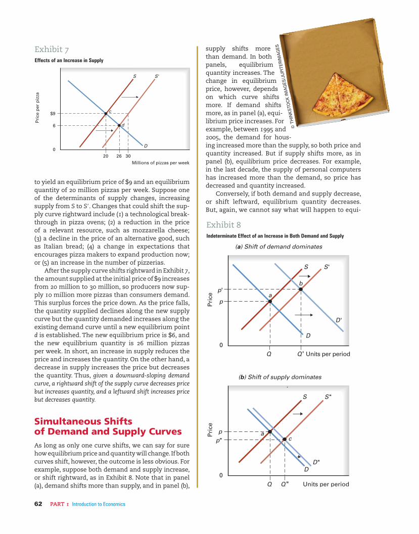
supply shifts more than demand. In both panels, equilibrium quantity increases. The change in equilibrium price, however, depends on which curve shifts more. If demand shifts more, as in panel (a), equi-librium price increases. For example, between 1995 and 2005, the demand for hous-ing increased more than the supply, so both price and quantity increased. But if supply shifts more, as in panel (b), equilibrium price decreases. For example, in the last decade, the supply of personal computers has increased more than the demand, so price has decreased and quantity increased.

Conversely, if both demand and supply decrease, or shift leftward, equilibrium quantity decreases. But, again, we cannot say what will happen to equi-

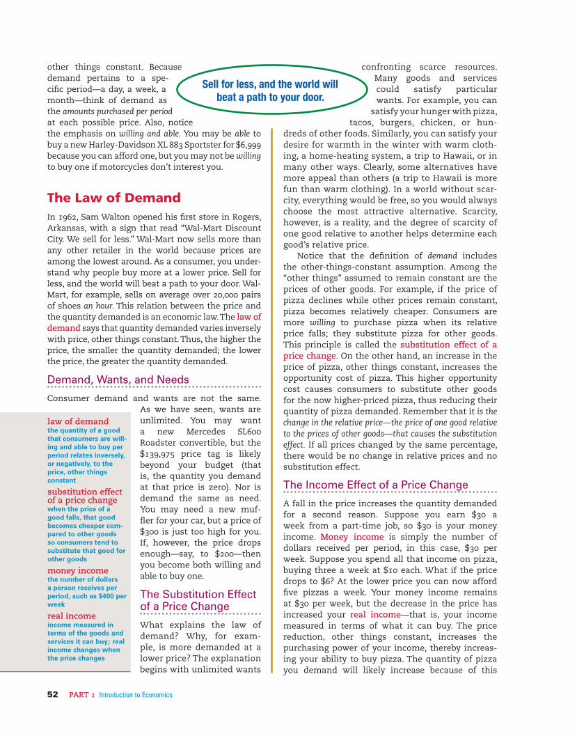
to yield an equilibrium price of $9 and an equilibrium quantity of 20 million pizzas per week. Suppose one of the determinants of supply changes, increasing supply from S to S�. Changes that could shift the sup-ply curve rightward include (1) a technological break-through in pizza ovens; (2) a reduction in the price of a relevant resource, such as mozzarella cheese; (3) a decline in the price of an alternative good, such as Italian bread; (4) a change in expectations that encourages pizza makers to expand production now; or (5) an increase in the number of pizzerias.

After the supply curve shifts rightward in Exhibit 7, the amount supplied at the initial price of $9 increases from 20 million to 30 million, so producers now sup-ply 10 million more pizzas than consumers demand. This surplus forces the price down. As the price falls, the quantity supplied declines along the new supply curve but the quantity demanded increases along the existing demand curve until a new equilibrium point d is established. The new equilibrium price is $6, and the new equilibrium quantity is 26 million pizzas per week. In short, an increase in supply reduces the price and increases the quantity. On the other hand, a decrease in supply increases the price but decreases the quantity. Thus, given a downward-sloping demand curve, a rightward shift of the supply curve decreases price but increases quantity, and a leftward shift increases price but decreases quantity.

Simultaneous Shifts of Demand and Supply CurvesAs long as only one curve shifts, we can say for sure how equilibrium price and quantity will change. If both curves shift, however, the outcome is less obvious. For example, suppose both demand and supply increase, or shift rightward, as in Exhibit 8. Note that in panel (a), demand shifts more than supply, and in panel (b),

Exhibit 7Effects of an Increase in Supply

20 26 30 Millions of pizzas per week

Pri

ce p

er p

izza

$9

6

0

S

D

c

d

S'

© T

HIN

KS

TOC

K IM

AG

ES/J

UPI

TER

IMA

GES

Exhibit 8Indeterminate Effect of an Increase in Both Demand and Supply

p'

p

0

Pri

ce

Q Q'

pp"

Pri

ce

Q Q" Units per period

Units per period

S S'

D'

D

DD"

S S"

(b) Shift of supply dominates

(a) Shift of demand dominates

0

a

a

b

c



athletes in the world—earning 60 percent more than pro baseball’s average and at least double that for pro football and pro hockey.

But rare talent alone does not command high pay. Top rodeo riders, top bowlers, and top women basket-ball players also possess rare talent, but the demand for their talent is not suffi cient to support pay any-where near NBA levels. Some sports aren’t even pop-ular enough to support professional leagues.

LO5 DisequilibriumA surplus exerts downward pressure on the price, and a shortage exerts upward pressure. Markets, however, don’t always reach equilibrium quickly. During the time required to adjust, the mar-ket is said to be in disequilibrium. Disequilibrium is usually temporary as the market gropes for equi-librium. But sometimes, often as a result of govern-ment intervention, disequilibrium can last a while, perhaps decades, as we will see next.

Price FloorsSometimes public offi cials set prices above their equi-librium levels. For example, the federal government regulates some agriculture

librium price unless we examine relative shifts. (You can use Exhibit 8 to consider decreases in demand and supply by viewing D� and S� as the initial curves.) If demand shifts more, the price will fall. If supply shifts more, the price will rise.

If demand and supply shift in opposite directions, we can say what will happen to equilibrium price. Equilibrium price will increase if demand increases and supply decreases. Equilibrium price will decrease if demand decreases and supply increases. Without reference to particular shifts, however, we cannot say what will happen to equilibrium quantity.

These results are no doubt confusing, but Exhibit 9 summarizes the four possible combinations of changes. Using Exhibit 9 as a reference, please take the time right now to work through some changes in demand and supply to develop a feel for the results.

The Market for Professional Basketball

Take a look at Exhibit 10 depicting the market for NBA players, with demand and supply in 1980 as D1980 and S1980. The intersection of these two curves generated an average pay in 1980 of $170,000, or $0.17 million, for the 300 or so players in the league. Since 1980, the talent pool expanded somewhat, shifting the supply curve a bit rightward from S1980 to S2007 (almost by defi nition, the supply of the top few hundred play-ers in the world is limited). But demand exploded from D1980 to D2007. With supply relatively fi xed, the greater demand boosted average pay for NBA play-ers to $4.9 million by 2007 for the 450 or so players in the league. Such pay attracts younger and younger players. NBA players are now the highest-paid team

Exhibit 9Effects of Shifts of Both Demand and Supply

Supplyincreases

Supplydecreases

Demand increases Demand decreases

Change in demand

Ch

an

ge

in

su

pp

ly

Equilibriumprice changeis indeterminate.

Equilibriumquantity increases.

Equilibriumprice rises.

Equilibriumquantity changeis indeterminate.

Equilibriumprice falls.

Equilibriumquantity changeis indeterminate.

Equilibrium pricechange is indeterminate.

Equilibriumquantity decreases.

Exhibit 10NBA Pay Leaps

450

1980 1980D S

$4.92007

2007D

S

300

$0.17

Players per season

Ave

rag

e p

ay p

er s

easo

n (m

illio

ns)

200100 400

4.0

3.0

2.0

1.0

disequilibriumthe condition that exists in a market when the plans of buyers do not match those of sellers; a temporary mismatch be-tween quantity supplied and quantity demanded as the market seeks equilibrium

© R

UB

BE

RB

ALL

/JU

PIT

ER

IMA

GE

S

Average annual pay $4.9 million.



ket, the government usually agrees to buy the surplus milk. The federal government, in fact, spends bil-lions buying and stor-ing surplus agricultural products. Note, to have an impact, a price fl oor must be set above the equilibrium price. A price fl oor set at or below the equilibrium price would be nonbinding (how come?). Price fl oors distort markets and reduce economic welfare.

Price CeilingsSometimes public offi cials try to keep a price below the equilibrium level by setting a price ceiling, or a maximum selling price. Concern about the rising cost of rental housing in some cities has prompted city offi cials to impose rent ceilings. Exhibit 11b depicts the demand and supply of rental housing. The ver-tical axis shows monthly rent, and the horizontal axis shows the quantity of rental units. The equilib-rium, or market-clearing, rent is $1,000 per month, and the equilibrium quantity is 50,000 housing units. Suppose city offi cials set a maximum rent of $600 per month. At that ceiling price, 60,000 rental units are demanded, but only 40,000 supplied, resulting in a housing shortage of 20,000 units. Because of the price ceiling, the rental price no longer rations hous-ing to those who value it the most. Other devices

prices in an attempt to ensure farmers a higher and more stable income than they would otherwise earn. To achieve higher prices, the federal government sets

a price fl oor, or a minimum selling price that is above the equilibrium price. Exhibit 11a shows the effect of a $2.50 per gallon price fl oor for milk. At that price, farmers supply 24 million gallons per week, but consumers demand only 14 million gallons, yielding a surplus of 10 million gallons. This surplus milk will pile up on store shelves, eventually souring. To take it off the mar-

price fl oora minimum legal price below which a product cannot be sold; to have an impact, a price fl oor must be set above the equilibrium price

price ceilinga maximum legal price above which a product cannot be sold; to have an impact, a price ceil-ing must be set below the equilibrium price

Rare talent alone doesn’t command high pay. Only the 300 or so top riders can earn a living. Only the top 50 or so make more than $100,000.

© H

AN

S-P

ET

ER

ME

RT

EN

/MA

UR

ITIU

S D

IE B

ILD

AG

EN

TU

R G

MB

H/P

HO

TOLI

BR

AR

Y

Exhibit 11aPrice Floors for Milk

$2.50

Pri

ce p

er g

allo

n

14 19 24

S

D

Millions of gallons per month

Surplus

1.90

0

Exhibit 11bPrice Ceilings for Rent

$1,000

600

Mo

nth

ly r

enta

l pri

ce

40 50 60

D

S

Shortage

Thousands of rental units per month

0

© T

HIN

KS

TOC

K IM

AG

ES/J

UPI

TER

IMA

GES



are consciously designed. Just as the law of gravity works whether or not we understand Newton’s prin-ciples, market forces operate whether or not partici-pants understand demand and supply. These forces arise naturally, much the way car dealers cluster on the outskirts of town to attract more customers.

Markets have their critics. Some observers may be troubled, for example, that an NBA star like Kevin Garnett earns a salary that could pay for 500 new schoolteachers, or that movie stars earn enough to pay for 1,000 new schoolteachers, or that U.S. con-sumers spend over $40 billion on their pets. On your next trip to the supermarket, notice how much shelf space goes to pet products—often an entire aisle. PetSmart, a chain store, sells over 12,000 pet items. Veterinarians offer cancer treatment, cataract removal, root canals, even acupuncture. Kidney dial-ysis for a pet can cost over $75,000 per year.

In a market economy, consumers are kings and queens. Consumer sovereignty rules, deciding what gets produced. Those who don’t like the market outcome usually look to government for a solution through price ceilings and price fl oors, regulations, income redistribution, and public fi nance more generally.

emerge to ration housing, such as long waiting lists, personal connections, and the willingness to make under-the-table payments, such as “key fees,” “fi nd-er’s fees,” high security deposits, and the like. To have an impact, a price ceiling must be set below the equilibrium price. A price ceiling set at or above the equilibrium level would be nonbinding. Price fl oors and ceilings distort markets and reduce economic welfare.

Government intervention is not the only source of market disequilibrium. Sometimes, when new products are introduced or when demand suddenly changes, it takes a while to reach equilibrium. For example, popular toys, best-selling books, and chart-busting CDs sometimes sell out. On the other hand, some new products attract few customers and pile up unsold on store shelves, awaiting a “clearance sale.”

Final WordDemand and supply are the building blocks of a mar-ket economy. Although a market usually involves the interaction of many buyers and sellers, few markets

Year that October was

designated National Pizza

Month. > 1987

Annual sales of the pizza industry. > $30 billion

< Slices per second rate at which

Americans eat pizza, which amounts to

approximately 100 acres of pizza

each day.

350

< Pizzerias in the United States.

69,000Amount of pizza each

man, woman, and child in America eats on average in a year. > 23 pounds

< Number of pizzas sold in the U.S. each year.

3 billion

SOURCES: Pizza Today magazine; National Association of Pizza Operators; http://pizzaware.com/facts.htm; Blumenfeld and Associates, Darien, CT; Packaged Facts, New York.

© T

HIN

KS

TOC

K IM

AG

ES

/JU

PIT

ER

IMA

GE

S


Date post:	08-Mar-2018
Category:	Documents
Upload:	vanduong
View:	231 times
Download:	4 times

Demand, Supply, Markets -...

Documents