DEMOGRAPHIC RESEARCH A peer-reviewed, open-access journal of population sciences DEMOGRAPHIC RESEARCH VOLUME 32, ARTICLE 19, PAGES 563–588 PUBLISHED 24 FEBRUARY 2015 http://www.demographic-research.org/Volumes/Vol32/19/ DOI: 10.4054/DemRes.2015.32.19 Research Article Demography and the statistics of lifetime economic transfers under individual stochasticity Hal Caswell Fanny Annemarie Kluge c 2015 Hal Caswell & Fanny Annemarie Kluge. This open-access work is published under the terms of the Creative Commons Attribution NonCommercial License 2.0 Germany, which permits use, reproduction & distribution in any medium for non-commercial purposes, provided the original author(s) and source are given credit. See http://creativecommons.org/licenses/by-nc/2.0/de/
Transcript
DEMOGRAPHIC RESEARCHA peer-reviewed, open-access journal of population sciences
DEMOGRAPHIC RESEARCH
VOLUME 32, ARTICLE 19, PAGES 563–588PUBLISHED 24 FEBRUARY 2015http://www.demographic-research.org/Volumes/Vol32/19/DOI: 10.4054/DemRes.2015.32.19
Research Article
Demography and the statistics of lifetimeeconomic transfers under individualstochasticity
This open-access work is published under the terms of the CreativeCommons Attribution NonCommercial License 2.0 Germany, which permitsuse, reproduction & distribution in any medium for non-commercialpurposes, provided the original author(s) and source are given credit.See http://creativecommons.org/licenses/by-nc/2.0/de/
4 Economic transfers for Germany 5694.1 Changes in economic transfers over time 5694.2 Sources of variance: fixed and random rewards 5734.3 The effects of education on lifetime economic transfers 5744.4 Effects of changes in the mortality schedule 5774.5 Completing the economic lifecycle: income, consumption, and deficit 580
5 Summary 583
6 Discussion 584
7 Acknowledgments 586
References 587
Demographic Research: Volume 32, Article 19
Research Article
Demography and the statistics of lifetime economic transfers underindividual stochasticity
Hal Caswell1
Fanny Annemarie Kluge2
Abstract
BACKGROUNDAs individuals progress through the life cycle, they receive income and consume goodsand services. The age schedules of labor income, consumption, and life cycle deficitreflect the economic roles played at different ages. Lifetime accumulation of economicvariables has been less well studied, and our goal here is to rectify that.
OBJECTIVETo derive and apply a method to compute the lifetime accumulated labor income, con-sumption, and life cycle deficit, and to go beyond the calculation of mean lifetime accu-mulation to calculate statistics of variability among individuals in lifetime accumulation.
METHODSTo quantify variation among individuals, we calculate the mean, standard deviation, co-efficient of variation, and skewness of lifetime accumulated transfers, using the theory ofMarkov chains with rewards (Caswell 2011), applied to National Transfer Account datafor Germany of 1978, and 2003.
RESULTSThe age patterns of lifetime accumulated labor income are relatively stable over time.Both the mean and the standard deviation of remaining lifetime labor income declinewith age; the coefficient of variation, measuring variation relative to the mean, increasesdramatically with age. The skewness becomes large and positive at older ages. Educa-tion level affects all the statistics. About 30% of the variance in lifetime income is dueto variance in age-specific income, and about 70% is contributed by the mortality sched-ule. Lifetime consumption is less variable (as measured by the CV) than lifetime laborincome.
1 Institute for Biodiversity and Ecosystem Dynamics, University of Amsterdam, 1090GE Amsterdam, TheNetherlands, and Biology Department MS-34, Woods Hole Oceanographic Institution, Woods Hole MA 02543U.S.A. E-Mail: [email protected] Max Planck Institute for Demographic Research, 18057 Rostock, Germany. E-Mail: [email protected].
Caswell & Kluge: Demography and the statistics of lifetime economic transfers under individual stochasticity
CONCLUSIONSWe conclude that demographic Markov chains with rewards can add a potentially valu-able perspective to studies of the economic lifecycle. The variation among individuals inlifetime accumulations in our results reflects individual stochasticity, not heterogeneityamong individuals. Incorporating heterogeneity remains an important problem.
1. Introduction
Many countries are in the midst of an age transition, following a trajectory from an agestructure dominated by the young, to an age structure with a large component in theproductive ages, and finally to a structure dominated by the old. Such a transition hasfar-reaching effects on the sustainability of public transfer systems, public pensions andhealth and long-term care budgets.
The ageing of populations has naturally focused attention on the relation betweendemography and the generational economy. The generational economy comprises pro-duction, consumption, sharing, and saving of resources across age (Lee and Mason 2011).Production (in the form of labor income) and consumption have received a great deal ofattention, and are being studied using data from National Transfer Accounts (NTA).
Labor income and consumption have generally been studied in two complementaryways. One is by comparisons of the age patterns of per capita income or consumption,jointly referred to as the economic lifecycle. The second is in terms of population ag-gregates, in which age-specific per capita income and consumption are weighted by thepopulation age distribution (Skirbekk, Loichinger, and Barakat 2012) to obtain values atthe population level.
The international and comparative National Transfer Account project (NTA; for moredetails see www.ntaccounts.org) presents data on age-specific economic variables suchas consumption, income, transfers, or assets. They include all possible actors, such asgovernments, families and firms, and are therefore able to combine the examination ofpublic and private redistribution of resources. Using these data, it is possible to picturethe economic life cycle of individuals and to study, for example, the impact of changes inthe age structure on the economy or the impact of institutional settings on the individualeconomic lifecycle. These studies are based on the idea that an individual has some levelof income, consumption, and deficit (the difference between income and consumption),and that, aggregated over a population, these generate transfers of resources among ageclasses. Studies of these transfers determine those periods in which labor income is in-sufficient to finance an individual’s consumption (i.e., periods of dependency), and howthose periods are changed by public and private transfers or asset-based reallocations,
including saving and investment (e.g., Lee 1994; Lee, Lee, and Mason 2006; Lee andMason 2011).
Our goal here is to introduce two new perspectives on the generational economy.First, we develop measures for the lifetime accumulation of income, consumption, anddeficit, as a consequence of the economic lifecycle. The accumulated values are obtainedby integrating age-specific income and consumption over age, taking into account theprobabilities of survival (or other transitions, if relevant). Such lifetime accumulationsare familiar in demography. An individual’s accumulated reproductive output is the totalfertility rate (TFR) if mortality is ignored, or the net reproductive rate (R0) if mortalityis incorporated (Caswell 2011). In our analysis here, the age schedules of income orconsumption take the place of the age schedule of fertility, and we will show how tocompute the lifetime accumulation of these economic measures.
Our second goal is to go beyond calculating expectations of lifetime accumulations(as, e.g., R0 is the expectation of lifetime reproduction) to examine variation, among in-dividuals, in lifetime accumulation. This variation exists for two reasons. Consider acohort of individuals, all experiencing exactly the same demographic rates and the samepatterns of income and consumption. Even though the rates are the same for all individ-uals, mortality is a stochastic process, and individuals will differ in how long they live.3
In addition, the income, consumption, and other variables accruing to an individual at agiven age are themselves random variables that can be characterized by their moments.So, even two identical individuals who live to identical ages will differ in their lifetimeaccumulation of economic variables. The variation in lifetime outcomes resulting fromthese processes is called individual stochasticity (Caswell 2009, 2011).
Individual stochasticity must not be confused with heterogeneity among individuals.Individual stochasticity produces variation among individuals that are all experiencingexactly the same age- or stage-dependent vital rates. Unobserved heterogeneity can actto amplify that variation, but its calculation requires models that include both observedand unobserved heterogeneity [e.g., frailty models in survival analysis (Caswell 2014a)].Empirical measures of the variation in accumulated rewards will reflect both individualstochasticity and heterogeneity; one of the values of our approach is its potential to sepa-rate the two sources of variation (Caswell 2011).
To quantify the effects of individual stochasticity, we will calculate the variance, stan-dard deviation, coefficient of variation, and skewness of lifetime accumulated economicvariables. Such information has potential uses in policy-related analyses. Calculationsbased solely on mean values provide no information on the risks associated with vari-able outcomes. Knowing the mean lifetime income or consumption does not reveal howvariable that accumulation will be among members of a cohort, and hence says nothingabout how common unusually high or unusually low values will be among members of
3In a multistate model, individuals would also differ in how long they spend in each state (Caswell 2006, 2009),but we know of no multistate economic transfer data from which to develop such models.
Caswell & Kluge: Demography and the statistics of lifetime economic transfers under individual stochasticity
a cohort. Skewness (the standardized third moment about the mean) provides extra in-formation beyond variance; positive skewness implies a distribution with a long positivetail, and negative skewness implies the opposite. A convenient reference point is that theexponential distribution has a skewness of 2. The approach we will introduce provides,if desired, all the moments of remaining lifetime accumulation, so kurtosis and otherfunctions of the higher moments could also be calculated if desired (Caswell 2011).
The results reported here, based on data from Germany, are the first exploration ofaccumulations over the economic lifecycle. As such, we have little to which to comparethem. We expect that if more examples are analyzed, patterns will begin to appear in thecomparative results.
Organization of the paper. In Section 2 we describe the German NTA data on whichour analyses will be based. In Section 3 we describe our methods, using results fromthe demographic version of the theory of Markov chains with rewards. In Section 4 wepresent a series of applications to German National Transfer Accounts data (Kluge 2011).We close with a discussion.
Notation. Matrices are denoted by upper-case bold symbols (e.g., P), vectors by lower-case bold symbols (e.g., ρ). Vectors are column vectors by default. The transpose of Pis PT. The vector 1 is a vector of ones. The diagonal matrix with the vector x on thediagonal and zeros elsewhere is denoted D(x). The expected value is denoted by E(·),the variance by V (·), the coefficient of variation by CV (·) and the skewness by Sk(·).The Hadamard, or element-by-element, product of matrices A and B is denoted by A◦B.Transition matrices of Markov chains are written in column-to-row orientation, and henceare column-stochastic.
2. Data
Our analyses are based on NTA estimates for Germany obtained from the German Incomeand Expenditure Surveys (Einkommens und Verbrauchsstichprobe, or EVS) of 1978 and2003. The EVS has been conducted by the Federal Statistical Office since 1978 at fiveyear intervals, and is based on a representative quota sample of Germany’s private house-holds. In 1978, the dataset included 46,941 households from the former Federal Republicof Germany alone. The 2003 wave includes around 50,000 households made up of some127,000 individuals; the scientific-use file is a 98 percent sample of the original data set.
The EVS includes a detailed account of income, consumption, savings, and assets.For three months, participating households keep a detailed book of household accountsthat covers every kind of potential income and expenditures. The survey is representa-tive of households with a monthly net income of less than 18,000 euros. Very wealthy
households, persons with no permanent residence, and individuals living in institutionsare not included. The number of oldest old individuals above age 85 is low, so we use theestimates only up until age 85.
From the EVS survey data we obtained the first three moments of age-specific laborincome, age-specific expenditure, and age-specific deficits, for ages 0–90. We combinedthese with period mortality schedules (both sexes combined) from the Human MortalityDatabase (2012) to formulate absorbing Markov chains with rewards.
3. Markov chains with rewards
We analyze lifetime accumulations using the approach introduced by Caswell (2011) ina study of lifetime reproductive output. This is based on the mathematical frameworkof Markov chains with rewards (MCWR), introduced by Howard (1960) in the contextof dynamic programming (see also, e.g., Benito 1982; Puterman 1994; Sladky and vanDijk 2005). An individual moves among states according to a finite-state Markov chain.In our case, the states consist of age classes, plus an absorbing state representing death.The probability of transition from age class i to age class i+ 1 is the survival probabilitypi, and the probability of transition from age class i to death is qi = 1 − pi. This age-classified structure leads to a particularly simple Markov chain, but the theory is equallyapplicable to more complicated stage-classified or multi-state models (Caswell 2011).
At each time, the individual collects a “reward” rij that depends on the transition,from state j to state i, realized at that time. The reward may be positive or negative; inour case, the rewards will represent income, consumption, or the deficit (the differencebetween income and consumption). We assume that no rewards accrue to individuals whohave reached the absorbing state.
The transition matrix of the absorbing Markov chain is, in general,
P =
(U 0M I
), (1)
where U is the transition matrix (dimension s×s) among transient states and M a matrixof mortality rates, with mij the probability of death from cause i in age class j. In ourcase, U has survival probabilities on the subdiagonal and zeros elsewhere,
Caswell & Kluge: Demography and the statistics of lifetime economic transfers under individual stochasticity
and M is a row vector of mortalities given by
M = 1T − 1TU. (3)
Provided that the dominant eigenvalue of U is less than 1, which we assume and whichis true for demographic applications, an individual beginning in any transient state willeventually be absorbed (i.e., will eventually die) with probability 1.
The rewards collected at a transition are, in general, random variables. Let the randomreward obtained by an individual moving from state j to state i be rij . Let the matrix4 ofthe kth moments of the rij be denoted Rk:
Rk =(E[rkij] )
. (4)
Define ρ as a vector whose entries are the accumulated rewards accruing to an individualstarting in each state of the Markov chain, and let ρk be the vector of the kth moments ofthe entries of ρ,
ρk =(E[ρki] )
. (5)
The calculation of the accumulated rewards proceeds in the “backwards” fashion fa-miliar from dynamic programming (Howard 1960). Choose some terminal time T , definet as the time remaining until this terminal time, and let ρ(t) be the reward yet to be accu-mulated at t. At the terminal time, no more rewards will be accumulated, so ρ(0) = 0.
Caswell (2011) showed that the first three moments of the accumulated reward satisfythe following system of equations:
ρ1(t+ 1) = (P ◦R1)T1+PTρ1(t) (6)
ρ2(t+ 1) = (P ◦R2)T1+ 2 (P ◦R1)
Tρ1(t) +PTρ2(t) (7)
ρ3(t+ 1) = (P ◦R3)T1+ 3 (P ◦R2)
Tρ1(t) + 3 (P ◦R1)
Tρ2(t) +PTρ3(t)(8)
for t = 0, . . . , T − 1, with ρ1(0) = ρ2(0) = ρ3(0) = 0. The moments of the lifetime ac-cumulated reward are obtained as the limt→∞ ρi(t). In practice, the system of equations(6)–(8) is iterated until the values converge, to obtain the vectors of moments of lifetimeaccumulation.
From these moment vectors we calculate some descriptive statistics of the lifetimeaccumulation, including the mean, standard deviation, coefficient of variation (CV) andskewness.
4In our notation, the expression ( xij ) denotes a matrix with xij in the ith row and jth column.
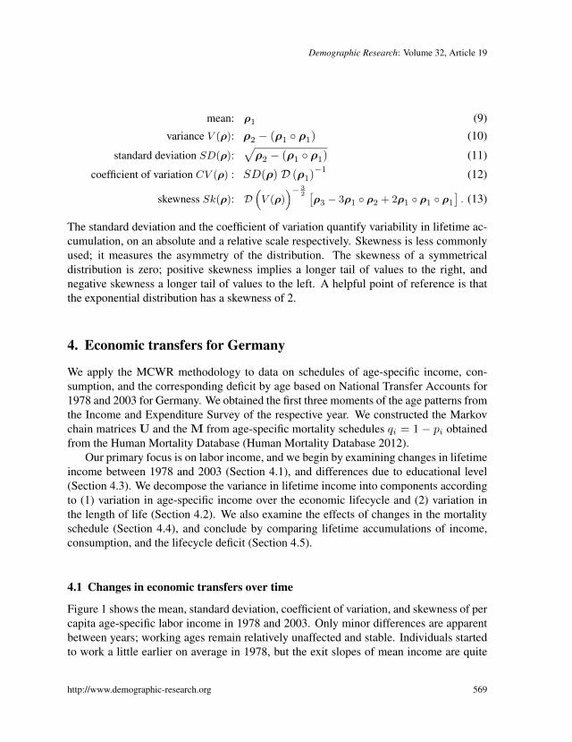
coefficient of variation CV (ρ) : SD(ρ) D (ρ1)−1 (12)
skewness Sk(ρ): D(V (ρ)
)− 32 [
ρ3 − 3ρ1 ◦ ρ2 + 2ρ1 ◦ ρ1 ◦ ρ1
]. (13)
The standard deviation and the coefficient of variation quantify variability in lifetime ac-cumulation, on an absolute and a relative scale respectively. Skewness is less commonlyused; it measures the asymmetry of the distribution. The skewness of a symmetricaldistribution is zero; positive skewness implies a longer tail of values to the right, andnegative skewness a longer tail of values to the left. A helpful point of reference is thatthe exponential distribution has a skewness of 2.
4. Economic transfers for Germany
We apply the MCWR methodology to data on schedules of age-specific income, con-sumption, and the corresponding deficit by age based on National Transfer Accounts for1978 and 2003 for Germany. We obtained the first three moments of the age patterns fromthe Income and Expenditure Survey of the respective year. We constructed the Markovchain matrices U and the M from age-specific mortality schedules qi = 1− pi obtainedfrom the Human Mortality Database (Human Mortality Database 2012).
Our primary focus is on labor income, and we begin by examining changes in lifetimeincome between 1978 and 2003 (Section 4.1), and differences due to educational level(Section 4.3). We decompose the variance in lifetime income into components accordingto (1) variation in age-specific income over the economic lifecycle and (2) variation inthe length of life (Section 4.2). We also examine the effects of changes in the mortalityschedule (Section 4.4), and conclude by comparing lifetime accumulations of income,consumption, and the lifecycle deficit (Section 4.5).
4.1 Changes in economic transfers over time
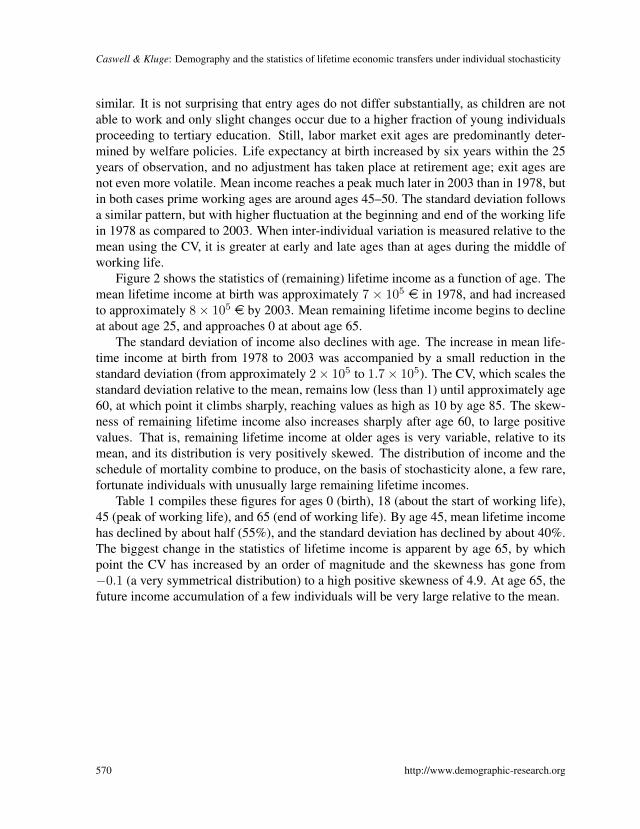
Figure 1 shows the mean, standard deviation, coefficient of variation, and skewness of percapita age-specific labor income in 1978 and 2003. Only minor differences are apparentbetween years; working ages remain relatively unaffected and stable. Individuals startedto work a little earlier on average in 1978, but the exit slopes of mean income are quite
Caswell & Kluge: Demography and the statistics of lifetime economic transfers under individual stochasticity
similar. It is not surprising that entry ages do not differ substantially, as children are notable to work and only slight changes occur due to a higher fraction of young individualsproceeding to tertiary education. Still, labor market exit ages are predominantly deter-mined by welfare policies. Life expectancy at birth increased by six years within the 25years of observation, and no adjustment has taken place at retirement age; exit ages arenot even more volatile. Mean income reaches a peak much later in 2003 than in 1978, butin both cases prime working ages are around ages 45–50. The standard deviation followsa similar pattern, but with higher fluctuation at the beginning and end of the working lifein 1978 as compared to 2003. When inter-individual variation is measured relative to themean using the CV, it is greater at early and late ages than at ages during the middle ofworking life.
Figure 2 shows the statistics of (remaining) lifetime income as a function of age. Themean lifetime income at birth was approximately 7 × 10⁵ e in 1978, and had increasedto approximately 8× 105 e by 2003. Mean remaining lifetime income begins to declineat about age 25, and approaches 0 at about age 65.
The standard deviation of income also declines with age. The increase in mean life-time income at birth from 1978 to 2003 was accompanied by a small reduction in thestandard deviation (from approximately 2× 10⁵ to 1.7× 10⁵). The CV, which scales thestandard deviation relative to the mean, remains low (less than 1) until approximately age60, at which point it climbs sharply, reaching values as high as 10 by age 85. The skew-ness of remaining lifetime income also increases sharply after age 60, to large positivevalues. That is, remaining lifetime income at older ages is very variable, relative to itsmean, and its distribution is very positively skewed. The distribution of income and theschedule of mortality combine to produce, on the basis of stochasticity alone, a few rare,fortunate individuals with unusually large remaining lifetime incomes.
Table 1 compiles these figures for ages 0 (birth), 18 (about the start of working life),45 (peak of working life), and 65 (end of working life). By age 45, mean lifetime incomehas declined by about half (55%), and the standard deviation has declined by about 40%.The biggest change in the statistics of lifetime income is apparent by age 65, by whichpoint the CV has increased by an order of magnitude and the skewness has gone from−0.1 (a very symmetrical distribution) to a high positive skewness of 4.9. At age 65, thefuture income accumulation of a few individuals will be very large relative to the mean.
Figure 1: Age schedules of the statistics of per capita income in Germany, in1978 and 2003(a) Mean age-specific income (e)(b) The standard deviation of income (e)(c) The coefficient of variation (CV) of income (dimensionless)(d) The skewness of income (dimensionless).
Caswell & Kluge: Demography and the statistics of lifetime economic transfers under individual stochasticity
Figure 2: Statistics of remaining lifetime accumulated income, as a functionof age, in Germany in 1978 and 2003(a) Mean lifetime income (e)(b) Standard deviation of lifetime income (e)(c) Coefficient of variation of lifetime income (dimensionless)(d) Skewness of lifetime income (dimensionless).
Table 1: The statistics of remaining lifetime income, as a function of age, forGermany in 1978 and 2003. Mean and standard deviationmeasured in units of 105 e. The coefficients of variation (CV) andskewness are dimensionless.
The variance among individuals in lifetime rewards has two sources. One is variationin the path taken through the life cycle (in this case, from initial age until death; in amultistate model, pathways could be more complex). The second is variation in the re-wards collected at each age. These two components can be partitioned by comparing theresults in Figure 2, which contain both components, with results obtained by fixing theage-specific rewards at their mean values (i.e., R2 = R1 ◦R1 and R3 = R1 ◦R1 ◦R1).When the rewards are fixed in this way, all variance is due to variation among pathways.
Figure 3 compares the standard deviation and skewness for fixed and random rewards,using the 2003 data. The standard deviation in lifetime income at birth is about 1.18 ×10⁵ e under the fixed reward model and about 1.71 × 10⁵ e under the random rewardmodel. In other words, ∼ 30% of the overall variance is due to the randomness of thereward pattern at each age, and about ∼ 70% is due to variation in the fate (i.e., age atdeath of the individuals.
Caswell & Kluge: Demography and the statistics of lifetime economic transfers under individual stochasticity
Figure 3: Standard deviation and skewness of remaining lifetimeaccumulated income, as a function of age, for Germany in 2003,calculated under the fixed reward model and the random rewardmodel.
0 20 40 60 800
2
4
6
8
10
12
14
16
18x 10
4
Age
Sta
ndar
d D
evia
tion
Life
time
Inco
me
2003
Random rewardFixed
0 20 40 60 80−6
−4
−2
0
2
4
6
8
10
AgeS
kew
Life
time
Inco
me
2003
Random rewardFixed
The difference in skewness is particularly noticeable. Including the variation in age-specific income schedule dramatically increases the skewness in remaining lifetime laborincome.
4.3 The effects of education on lifetime economic transfers
Education is known to affect levels of income (Miller 1960; Becker and Chiswick 1966;Hause 1975) as does occupation (Wilkinson 1966). Here we examine effects of educationon the statistics of lifetime accumulated income. Lifetime earnings are known to play animportant role in intergenerational mobility (Dunn 2007). We calculated lifetime laborincome using data from the EVS 2003 survey, classifying individuals into high, mediumand low educational attainment categories. We grouped individuals without a completeddegree in the low education category. All individuals having attained university or Fach-hochschule fall in the high education category. The remaining individuals are groupedinto medium education.
Figure 4 shows the mean, standard deviation, CV, and skewness of age-specific laborincome for the low, medium, and high education level categories. As expected, meanage-specific income at any age increases with increasing educational level. The standarddeviation follows the same pattern, so the CV is very similar for all three groups. Theskewness for the low and medium education groups follows the pattern familiar fromFigure 1. Skewness of age-specific income for the high education group is negative overmuch of working life, and is close to zero at older ages.
Figure 4: The age schedules of per capita age-specific income for low,medium, and high educational levels, from age 18 onward. Meanand standard deviation in e; CV and skewness are dimensionless.
0 20 40 60 800
0.5
1
1.5
2
2.5
3
3.5x 10
4
Age
Mea
n In
com
e
LowMedHigh
0 20 40 60 800
0.5
1
1.5
2
2.5
3x 10
4
AgeS
D In
com
e
LowMedHigh
0 20 40 60 800
5
10
15
20
25
30
35
Age
CV
Inco
me
LowMedHigh
0 20 40 60 80−10
0
10
20
30
40
Age
Ske
wne
ss In
com
e
LowMedHigh
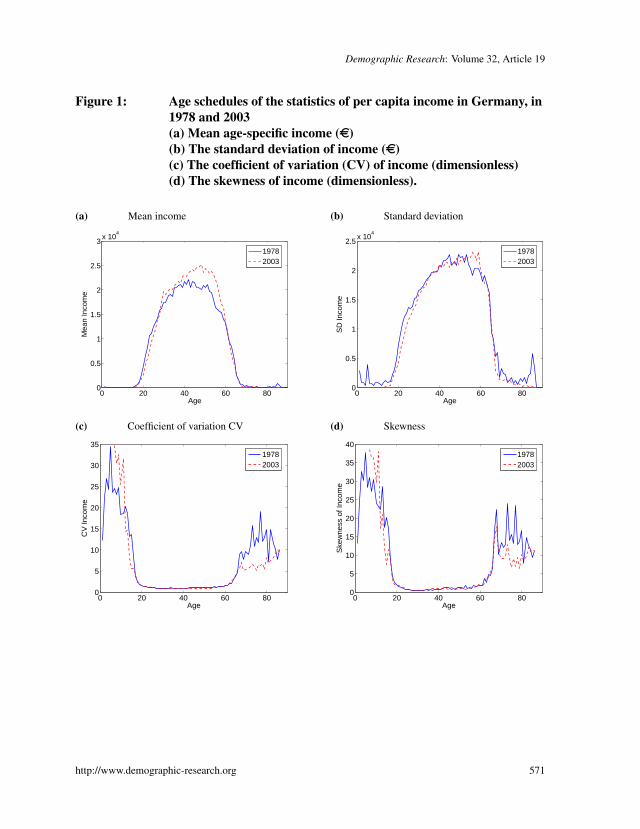
The results for lifetime accumulated income are shown in Figure 5. The patterns ofmean lifetime income are similar across all three education groups. The standard devi-ation declines with age, so the CV differs little among education groups, and follows apattern similar to that shown in Figure 2. As shown in Table 2, at age 18, mean lifetimeincome is roughly doubled, going from low to medium education, and increased by an-other 40% going from medium to high education levels. The proportional differences atage 45 are similar (about 70% increase from low to medium, and again from medium tohigh). The benefit of high education levels for mean lifetime income are even greater atage 65 (almost doubled compared to medium education).
Caswell & Kluge: Demography and the statistics of lifetime economic transfers under individual stochasticity
Figure 5: Statistics of lifetime accumulation of income for low, medium, andhigh educational levels, from age 18 onward. Mean and standarddeviation in e; CV and skewness are dimensionless.
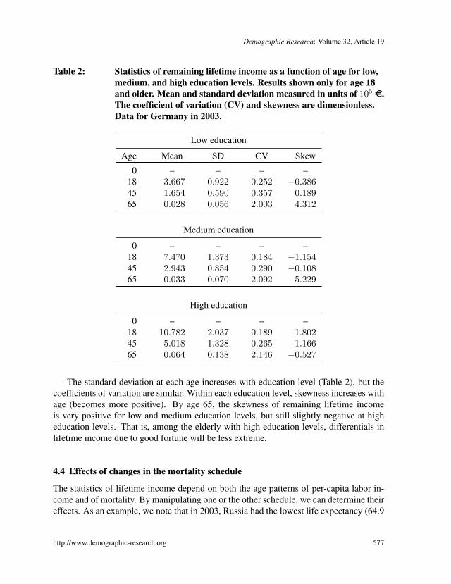
Table 2: Statistics of remaining lifetime income as a function of age for low,medium, and high education levels. Results shown only for age 18and older. Mean and standard deviation measured in units of 105 e.The coefficient of variation (CV) and skewness are dimensionless.Data for Germany in 2003.
The standard deviation at each age increases with education level (Table 2), but thecoefficients of variation are similar. Within each education level, skewness increases withage (becomes more positive). By age 65, the skewness of remaining lifetime incomeis very positive for low and medium education levels, but still slightly negative at higheducation levels. That is, among the elderly with high education levels, differentials inlifetime income due to good fortune will be less extreme.
4.4 Effects of changes in the mortality schedule
The statistics of lifetime income depend on both the age patterns of per-capita labor in-come and of mortality. By manipulating one or the other schedule, we can determine theireffects. As an example, we note that in 2003, Russia had the lowest life expectancy (64.9
Caswell & Kluge: Demography and the statistics of lifetime economic transfers under individual stochasticity
years) of any country in the Human Mortality Database; more than 15 years less than thatof Germany. To see the effects that such mortality differences might have, we fixed theage pattern of income at the values for EVS 2003, and substituted the Russian mortalityschedule for that of Germany.
The results are shown in Figure 6 and Table 3. The higher mortality schedule ofRussia reduces mean lifetime income by about 12% and the standard deviation by about35%. The differences in the CV and skewness of lifetime income are minor. This mayreflect the fact that individuals usually stop working by age 65, whereas the differencesin life expectancy between the two countries are due to differences in mortality outsidethe working years of life.
Figure 6: Statistics of remaining lifetime accumulated income, as a functionof age, using the reward schedule for Germany in 2003 and themortality schedules of Germany and of Russia in 2003. Mean andstandard deviation in e; CV and skewness are dimensionless.
Table 3: Statistics of remaining lifetime income as a function of age, for ahypothetical scenario combining the income data for Germany in2003 with the mortality levels of Russia in that year. Mean andstandard deviation measured in units of 105 e. The coefficient ofvariation (CV) and skewness are dimensionless.
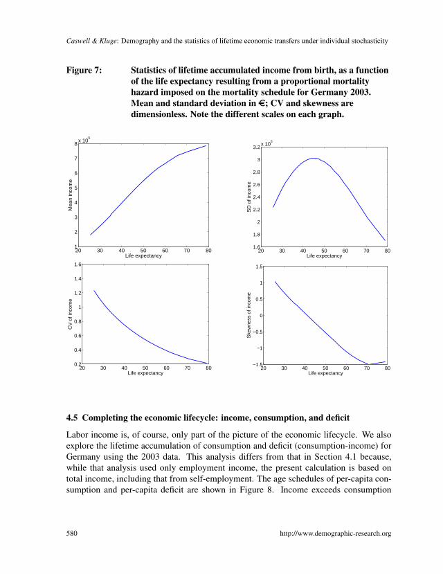
As a further exploration of the effects of mortality, we manipulated the 2003 mortalityschedule of Germany by imposing an additional proportional hazard, thus maintainingthe shape of the mortality schedule, while reducing life expectancy. Figure 7 showslifetime accumulated income as a function of the life expectancy at birth of the modifiedmortality schedule. As expected, mean lifetime income increases with life expectancy.The standard deviation reaches a peak at intermediate mortality levels and declines atvery low or very high life expectancies. The CV and skewness of lifetime income bothdecline as mortality declines, but the changes are modest (note the y-axis scales).
Caswell & Kluge: Demography and the statistics of lifetime economic transfers under individual stochasticity
Figure 7: Statistics of lifetime accumulated income from birth, as a functionof the life expectancy resulting from a proportional mortalityhazard imposed on the mortality schedule for Germany 2003.Mean and standard deviation in e; CV and skewness aredimensionless. Note the different scales on each graph.
20 30 40 50 60 70 801
2
3
4
5
6
7
8x 10
5
Life expectancy
Mea
n in
com
e
20 30 40 50 60 70 801.6
1.8
2
2.2
2.4
2.6
2.8
3
3.2x 10
5
Life expectancy
SD
of i
ncom
e
20 30 40 50 60 70 800.2
0.4
0.6
0.8
1
1.2
1.4
1.6
Life expectancy
CV
of i
ncom
e
20 30 40 50 60 70 80−1.5
−1
−0.5
0
0.5
1
1.5
Life expectancy
Ske
wne
ss o
f inc
ome
4.5 Completing the economic lifecycle: income, consumption, and deficit
Labor income is, of course, only part of the picture of the economic lifecycle. We alsoexplore the lifetime accumulation of consumption and deficit (consumption-income) forGermany using the 2003 data. This analysis differs from that in Section 4.1 because,while that analysis used only employment income, the present calculation is based ontotal income, including that from self-employment. The age schedules of per-capita con-sumption and per-capita deficit are shown in Figure 8. Income exceeds consumption
during the peak working years, but at earlier and later years, the income is less thanconsumption and the deficit is positive.
Figure 8: Statistics of the age schedules of production, consumption, anddeficit for Germany in 2003. Mean and standard deviation in e;CV and skewness are dimensionless. Coefficient of variation is notshown for deficit because the CV is defined only for non-negativequantities.
0 10 20 30 40 50 60 70 80 90−2
−1
0
1
2
3
4x 10
4
Age
Mea
n
IncomeConsumptionDeficit
0 10 20 30 40 50 60 70 80 900
0.5
1
1.5
2
2.5
3
3.5x 10
4
Age
Sta
ndar
d de
viat
ion
IncomeConsumptionDeficit
0 10 20 30 40 50 60 70 80 900
5
10
15
20
25
30
35
40
Age
Coe
ffici
ent o
f var
iatio
n
IncomeConsumption
0 10 20 30 40 50 60 70 80 90−10
−5
0
5
10
15
20
25
30
35
40
Age
Ske
wne
ss
IncomeConsumptionDeficit
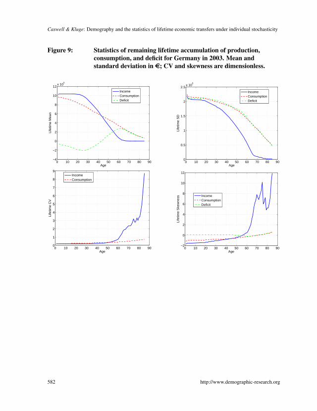
The statistics of the remaining lifetime accumulation of these, as a function of age,are shown in Figure 9 and summarized in Table 4. At birth, expected lifetime incomeslightly exceeds expected lifetime consumption. The expectations of remaining lifetimeincome and of consumption both decline with age, producing a negative, and then (afterage 45) positive expected lifetime deficit. The standard deviations of all three quantitiesdecline with age.
Caswell & Kluge: Demography and the statistics of lifetime economic transfers under individual stochasticity
Figure 9: Statistics of remaining lifetime accumulation of production,consumption, and deficit for Germany in 2003. Mean andstandard deviation in e; CV and skewness are dimensionless.
Table 4: Statistics of remaining lifetime income, consumption, and deficit, asa function of age, for Germany in 2003. Mean and standarddeviation measured in units of 105 e. Coefficient of variation (CV)and skewness are dimensionless; CV of deficit is not shown, becauseit is defined only for non-negative quantities.
Our results are new insights from a new approach. Here, we briefly list our major findings.
1. Markov chains with rewards can be used to extend the demographic calculationof the statistics of lifetime reproduction to exactly parallel statistics of lifetimeincome, consumption, and deficit.
2. The age patterns of the mean, standard deviation, coefficient of variation, and skew-ness of lifetime are consistent across different times, differences in educationallevels, and changes in mortality. This suggests that these patterns are a consistentresult of the schedules of age-specific income and of age-specific mortality.
Caswell & Kluge: Demography and the statistics of lifetime economic transfers under individual stochasticity
3. About 30% of the variance in lifetime income is due to variation in age-specificincome, and about 70% is due to variation in the fate of individuals.
4. Changes in the skewness of remaining lifetime income are dramatic: skewness issmall and negative over much of life, but by age 65 it becomes large and positive,on the order of 4–6. This is even more skewed than an exponential distribution,which has a constant skewness of 2. The only exception we found is for the higheducation group, where skewness at age 65 is about−0.5. Otherwise, demographicforces produce lifetime income for 50-year olds characterized by a long tail ofpositive deviations.
6. Discussion
The connection between the age-specific schedules and lifetime accumulations has provenvaluable in several disparate areas of demography. When age-specific survivorship is in-tegrated forward the result is life expectancy. When age-specific fertility is integratedforward, the result is the net reproductive rateR0 or the total fertility rate TFR, dependingon whether or not mortality is included. When the age schedule of disability prevalenceis integrated forward, the result is healthy life expectancy.
We can now add to this list the calculation of lifetime accumulations of economicvariables. The analysis is not limited to income, consumption, and deficit; any variablesfor which age-specific schedules are available can be analyzed with this model. Theextension from expected values to measures of variance and skewness may add an extradimension to policy decisions, because only by accounting for variability can the risk ofpolicy decisions be incorporated.
The results of our examples provide suggestive insights into the importance of ran-domness for economic events. The results summarized in Tables 1–4 reveal some pat-terns.
1. Labor income. The mean declines almost monotonically from birth to the end oflife (not surprising). The standard deviation also declines, but more slowly, so thatthe CV increases dramatically with age, by about an order of magnitude betweenages 45 and 65. The skewness is slightly negative until older ages; by 65 it hasbecome large and positive. This holds true even if mortality is increased, either byusing the Russian mortality schedule with its low life expectancy, or by imposingan age-independent proportional hazard. Lifetime income appears to behave differ-ently at high levels of education, in which the skewness remains slightly negativeeven at age 65.
2. Consumption. The patterns for consumption differ from those for income. Themean and standard deviation both decrease with age, but not as much as is true for
income. The CV remains relatively low. Skewness remains negative and small.Thus the distribution of consumption appears to be much more symmetrical at oldages than is that of income.
3. Deficit. The mean of the remaining lifetime deficit increases with age. It is negative(i.e., lifetime income will exceed consumption) from birth to age 18, and becomespositive as an individual approaches the end of working life. The standard deviationof lifetime deficit decreases slightly, and the skewness, never very great, becomesslightly negative at the end of life.
The calculation of these lifetime statistics, following equations (6)–(8), requires thefollowing data.
1. An age-specific schedule of mortality or, in the stage-classified case, a transitionmatrix among stages, including the stage-specific mortality rate. Together, thesedata specify the Markov chain transition matrix P in equation (1).
2. The moments of the reward associated with each stage transition, expressed as thereward matrices Rk in equation (4). Measuring these moments requires individual-level data. In the absence of such data, the moments can be modelled by assumingan appropriate distribution; cf., calculations of lifetime reproductive output using aPoisson assumption; (Caswell 2011).
3. We note also that lifetime accumulation is sometimes discounted as an estimate ofthe net present value of a specific variable. This is done, for example , to calculatethe net present value of public transfers by cohorts (Bommier et al. 2010). Althoughwe did not discount values in this analysis, it could easily be incorporated. Equa-tions (66)–(69) in Caswell (2011) incorporate a discount factor 0 < β < 1; theseequations would replace equations (6)–(8) above for calculations of discounted re-wards.
Our results are the first to be calculated for any country. We hope that further analyseswill permit comparative studies that will help to understand the patterns.
The role of individual stochasticity. The variance in lifetime accumulation exists eventhough every individual experiences the same age-specific schedules of mortality and re-wards. Therefore, no heterogeneity appears in the calculations; instead the variances wereport here are due strictly to the individual stochasticity implied by the demographic pa-rameters and the distributions of age-specific rewards. These results provide a baselineagainst which observed variation can be compared, to quantify the effects of heterogene-ity that no doubt operates in real populations.
Note that age is the only i-state variable (Metz and Diekmann 1986; Caswell 2001,Sec. 3.1) to appear in these calculations. Therefore, the rewards accumulated at one
Caswell & Kluge: Demography and the statistics of lifetime economic transfers under individual stochasticity
age are independent of the rewards accumulated at the previous age. If they were not,individuals would experience different conditions depending on some property other thanage. It is as if an individual may, conditional on survival, randomly sample the pseudo-lives of different individuals: at age x collecting the income of a wealthy banker, at agex+ 1 the income of an unemployed factory worker, and so on.5
This may seem strange, because individuals do not really do this, but it is an un-avoidable assumption of a solely age-dependent model. Demography is replete with suchcalculations. Calculations of TFR or R0 assume that a woman at age x may become amother, then at x+ 1 become a mother again or not, independently of her previous expe-rience. The accumulation of lifetime reproduction is the result of a random walk amongthese lives. Calculations of healthy life expectancy from prevalence data by the Sulli-van method (Jagger et al. 2006) assume that an indivdidual at age x might be a disablednursing home resident, and at age x+ 1 a healthy marathon runner, and so on. The accu-mulation of healthy years is a random walk among the lives of individuals experiencingsome specified levels of health and disability.
The common structure of all these calculations is that the only source of heterogeneityincluded as an i-state variable is age. The transitions between banker and factory worker,or between nursing home resident and marathon runner, seem strange because they callon our belief that age is not the only factor involved.
The resolution of the paradox would be, in each case, to create a multi-state modelcombining age and employment status, or age and health status, or age and parity as i-state variables. Such models can capture the dynamic dependence of the heterogeneitythat leads to differences in rewards (see Rogers, Rogers, and Branch 1989 for a discussionof multistate models in health expectancy). When appropriate data are available, ouranalysis can be applied directly to them (e.g., Caswell 2014b for an age-parity model forfertility rewards).
7. Acknowledgments
This research was supported by ERC Advanced Grant 322989 and NSF Grant DEB-1257545. HC acknowledges the hospitality of the Max Planck Institute for DemographicResearch. The comments of two anonymous reviewers helped to improve an earlier ver-sion of the manuscript.
5We owe this delightful image to an anonymous reviewer.
Becker, G.S. and Chiswick, B.R. (1966). Education and the distribution of earnings. TheAmerican Economic Review 56(1/2): 358–369.
Benito, F. (1982). Calculating the variance in Markov-processes with random reward.Trabajos de estadıstica y de investigacion operativa 33(3): 73–85. doi:10.1007/BF02888435.
Bommier, A., Lee, R., Miller, T., and Zuber, S. (2010). Who wins and who loses? Publictransfer accounts for the US generations born 1850 to 2090. Population and Develop-ment Review 36(1): 1–26. doi:10.1111/j.1728-4457.2010.00315.x.
Caswell, H. (2001). Matrix population models: construction, analysis, and interpreta-tion. Sunderland, MA: Sinauer Associates, 2nd ed.
Caswell, H. (2006). Applications of Markov chains in demography. In: Langville,A.N. and Stewart, W.J. (eds.). MAM2006: Markov Anniversary Meeting. Raleigh, NC:Boson-Books: 319–334.
Caswell, H. (2009). Stage, age and individual stochasticity in demography. Oikos118(12): 1763–1782. doi:10.1111/j.1600-0706.2009.17620.x.
Caswell, H. (2011). Beyond R0: Demographic models for variability of lifetime repro-ductive output: demographic models for variability of lifetime reproductive output.PLOS ONE 6(6): e20809. doi:10.1371/journal.pone.0020809.
Caswell, H. (2014a). A matrix approach to the Gamma-Gompertz and related mortalitymodels. Demographic Research 31(19): 553–592. doi:10.4054/DemRes.2014.31.19.
Caswell, H. (2014b). Statistics of inter-individual variation in lifetime fertility: a Markovchain approach. Paper presented at the Annual Meeting of Population Association ofAmerica, Boston, MA, May 1–3 2014.
Dunn, C.E. (2007). The intergenerational transmission of lifetime earnings: Evi-dence from Brazil. The BE Journal of Economic Analysis & Policy 7(2): Article 2.doi:10.2202/1935-1682.1782.
Hause, J.C. (1975). Ability and schooling as determinants of lifetime earnings, or ifyou’re so smart, why aren’t you rich? In: Juster, F.T. (ed.). Education, Income, andHuman Behavior. New York: McGraw-Hill: 123–150.
Human Mortality Database (2012). University of California, Berkeley (USA), andMax Planck Institute for Demographic Research (Germany). [electronic resource].
Caswell & Kluge: Demography and the statistics of lifetime economic transfers under individual stochasticity
www.mortality.org.
Jagger, C., Cox, B., Le Roy, S., and EHEMU (2006). Health expectancy calculation bythe Sullivan method: a practical guide. EHEMU. (EHEMU Technical Report 2006 3).
Kluge, F.A. (2011). The individual economic lifecycle and its fiscal implications in anaging Germany – Findings from National Transfer Accounts. [PhD Thesis]. Rostock:University of Rostock.
Lee, R.D. (1994). The formal demography of population aging, transfers, and the eco-nomic life cycle. In: Martin, L.G. and Preston, S.H. (eds.). Demography of aging.Washington, DC: National Academy Press: 8–49.
Lee, R.D., Lee, S.H., and Mason, A. (2006). Charting the economic life cycle. In:Prskawetz, A., Bloom, D.E., and Lutz, W. (eds.). Population aging, human capitalaccumulation, and productivity growth. New York, Population Council: Populationand Development Review: 208–237. doi:10.3386/w12379.
Lee, R.D. and Mason, A. (2011). Population aging and the generational economy: aglobal perspective. Cheltenham, UK: Edward Elgar Pub.
Metz, J.A.J. and Diekmann, O. (1986). The dynamics of physiologically structured pop-ulations. Berlin: Springer-Verlag. doi:10.1007/978-3-662-13159-6.
Miller, H. (1960). Annual and lifetime income in relation to education: 1939–1959. TheAmerican Economic Review 50(5): 962–986.
Puterman, M.L. (1994). Markov decision processes: Discrete dynamic stochastic pro-gramming. New York, NY: John Wiley. doi:10.1002/9780470316887.
Rogers, A., Rogers, R.G., and Branch, L.G. (1989). A multistate analysis of active lifeexpectancy. Public Health Reports 104(3): 222–226.
Skirbekk, V., Loichinger, E., and Barakat, B.F. (2012). The aging of the workforce inEuropean countries. In: Hedge, J.W. and Borman, W.C. (eds.). The Oxford Handbookof work and aging. New York: Oxford University Press: 60–79. doi:10.1093/oxfordhb/9780195385052.013.0046.
Sladky, K. and van Dijk, N.M. (2005). Total reward variance in discrete and continu-ous time Markov chains. In: Fleuren, H., den Hertog, D., and Kort, P. (eds.). Op-erations Research Proceedings 2004. New York: Springer: 319–326. doi:10.1007/3-540-27679-3 40.
Wilkinson, B.W. (1966). Present values of lifetime earnings for different occupations.The Journal of Political Economy 74(6): 556–572. doi:10.1086/259220.