50
de.NBI Nanopore Training Course Documentation Release latest Sep 27, 2019

de.NBI Nanopore Training CourseDocumentation
Release latest
Sep 27, 2019


Contents
1 The Tutorial Data Set 3
2 Basecalling 52.1 Inspect the fast5 files . . . . . . . . . . . . . . . . . . . . . . . . . . . . . . . . . . . . . . . . . . . 52.2 Basecalling with Guppy . . . . . . . . . . . . . . . . . . . . . . . . . . . . . . . . . . . . . . . . . 72.3 Inspect the output . . . . . . . . . . . . . . . . . . . . . . . . . . . . . . . . . . . . . . . . . . . . 102.4 The results with complete data . . . . . . . . . . . . . . . . . . . . . . . . . . . . . . . . . . . . . . 112.5 Merge fastqs . . . . . . . . . . . . . . . . . . . . . . . . . . . . . . . . . . . . . . . . . . . . . . . 11
3 Data Quality Assessment 133.1 MinIONQC . . . . . . . . . . . . . . . . . . . . . . . . . . . . . . . . . . . . . . . . . . . . . . . . 133.2 FastQC . . . . . . . . . . . . . . . . . . . . . . . . . . . . . . . . . . . . . . . . . . . . . . . . . . 143.3 Generating Error Profiles . . . . . . . . . . . . . . . . . . . . . . . . . . . . . . . . . . . . . . . . . 18
4 Assembly 254.1 Assembly with canu . . . . . . . . . . . . . . . . . . . . . . . . . . . . . . . . . . . . . . . . . . . 254.2 Assembly evaluation with QUAST . . . . . . . . . . . . . . . . . . . . . . . . . . . . . . . . . . . 284.3 Assembly Graph inspection with bandage . . . . . . . . . . . . . . . . . . . . . . . . . . . . . . . . 284.4 Quality control by mapping . . . . . . . . . . . . . . . . . . . . . . . . . . . . . . . . . . . . . . . 29
5 Assembly polishing 315.1 Assembly polishing with pilon . . . . . . . . . . . . . . . . . . . . . . . . . . . . . . . . . . . . . . 315.2 Assembly polishing with racon and medaka . . . . . . . . . . . . . . . . . . . . . . . . . . . . . . . 355.3 Assembly polishing with nanopolish . . . . . . . . . . . . . . . . . . . . . . . . . . . . . . . . . . . 41
6 Genome annotation 456.1 Annotating the genome with prokka . . . . . . . . . . . . . . . . . . . . . . . . . . . . . . . . . . . 45
i

ii

de.NBI Nanopore Training Course Documentation, Release latest
Welcome to the two-day nanopore training course. This tutorial will guide you through the typical steps of a nanoporeassembly of a microbial genome.
Contents 1

de.NBI Nanopore Training Course Documentation, Release latest
2 Contents

CHAPTER 1
The Tutorial Data Set
The first thing you need to do is to connect to your virtual machine with the X2Go Client. If you are working withyour laptop and haven’t installed it yet - you can get it here: https://wiki.x2go.org/doku.php/download:start
Enter the IP of your virtual machine, the port, the username “ubuntu” and select your ssh key. When you havesuccessfully connected to your machine, open a terminal.
As you have started the VM with a volume attached, this volume needs to be given to the ubuntu user for easy access:
sudo chown ubuntu:ubuntu /mnt/volume/
Create a link in your home directory to the mounted volume:
ln -s /mnt/volume/ workdir
The tutorial dataset is located in our object store. We have also prepared some precomputed results.You can get bothhere (Group 1):
cd ~/workdirwget https://openstack.cebitec.uni-bielefeld.de:8080/swift/v1/nanopore_course_data/→˓Data_Group1.tar.gzwget https://openstack.cebitec.uni-bielefeld.de:8080/swift/v1/nanopore_course_data/→˓Results_Group1.tar.gz
. . . and for Group 2:
cd ~/workdirwget https://openstack.cebitec.uni-bielefeld.de:8080/swift/v1/nanopore_course_data/→˓Data_Group2.tar.gzwget https://openstack.cebitec.uni-bielefeld.de:8080/swift/v1/nanopore_course_data/→˓Results_Group2.tar.gz
Then, unpack the tar archive:
3

de.NBI Nanopore Training Course Documentation, Release latest
tar -xzvf Data_Group1.tar.gztar -xzvf Results_Group1.tar.gz
or
tar -xzvf Data_Group2.tar.gztar -xzvf Results_Group2.tar.gz
and remove the tar archives:
rm Data_Group1.tar.gzrm Results_Group1.tar.gzorrm Data_Group2.tar.gzrm Results_Group2.tar.gz
Have a short look, on what is contained within the data directory:
ls -l ~/workdir/data/-rw-r--r-- 1 ubuntu ubuntu 4372654 Aug 30 08:24 Reference.fnadrwxr-xr-x 2 ubuntu ubuntu 24576 Aug 30 08:24 fast5drwxrwxr-x 2 ubuntu ubuntu 4096 Sep 5 07:23 fast5_smalldrwxrwxr-x 2 ubuntu ubuntu 4096 Sep 12 08:01 fast5_tinydrwxr-xr-x 2 ubuntu ubuntu 4096 Aug 30 08:36 illumina
There are three folders with Nanopore fast5 data, a Reference genome for later comparisons and some illumina data.
If you want to disable system beep sounds:
xset -b
4 Chapter 1. The Tutorial Data Set

CHAPTER 2
Basecalling
We will perform a basecalling of the raw data with guppy.
2.1 Inspect the fast5 files
The raw signals in Nanopore sequencing are stored in HDF5 format. HDF stands for “Hierarchical Data Format”, andit is quite similar to json. Terms used by HDF include Groups, Attributes and Datasets. A Group can contain Groupsor Datasets and may have Attributes. A Dataset contains an array of datapoints. The way HDF5 is stored allows it toaccess individual Groups within the dataset fast and efficient.
The HDF5 tools can be used to display contents of HDF5 files. We will use two of them to explore our data:
h5dump -- Enables a user to examine the contents of an HDF5 file and dump those→˓contents to an ASCII file.h5ls -- Lists specified features of HDF5 file contents.
In order to get the complete content of a fast5 in readable form, you can use:
h5dump data/fast5_tiny/GXB01322_20181217_FAK35493_GA10000_sequencing_run_Run00014_→˓MIN106_RBK004_46674_0.fast5 | more
Inspect the output. The file starts with a root group:
GROUP "/" {[...]
followed by the first read:
GROUP "read_0061d165-af04-4c39-ad5e-8c4ebe3caa80" {[...]
at some point, the actual data is stored as a dataset:
5

de.NBI Nanopore Training Course Documentation, Release latest
DATASET "Signal" {DATATYPE H5T_STD_I16LEDATASPACE SIMPLE { ( 104805 ) / ( H5S_UNLIMITED ) }DATA {(0): 450, 414, 428, 435, 445, 439, 439, 416, 432, 437, 410, 403,(12): 429, 410, 415, 426, 424, 409, 415, 416, 422, 421, 422, 418,[...]
To get an overview on all reads, you could use the h5ls command:
h5ls data/fast5_tiny/GXB01322_20181217_FAK35493_GA10000_sequencing_run_Run00014_→˓MIN106_RBK004_46674_0.fast5
This will give you a list of all reads:
read_0061d165-af04-4c39-ad5e-8c4ebe3caa80 Groupread_00e09394-e199-4738-bf1a-2d2f97dff4a8 Groupread_01204611-3592-419c-9785-83c0fafa4c4a Groupread_0130da91-b3ad-42bd-847e-0d2ce314ee48 Groupread_015af2b6-ef6c-4c86-b598-02325d42fc6d Groupread_01a509fd-a58c-4257-8136-600c22b4d053 Groupread_01ed0343-0286-42f1-8ea3-0904d66521b6 Groupread_025147d4-e101-426c-8b80-38d752d41dc8 Group[...]
Which you can simply count to get the number of reads in your fast5 file:
h5ls data/fast5_tiny/GXB01322_20181217_FAK35493_GA10000_sequencing_run_Run00014_→˓MIN106_RBK004_46674_0.fast5 | wc -l
In order to inspect what is stored for an individual read, you can specify that read, as if it were a directory using h5ls:
h5ls data/fast5_tiny/GXB01322_20181217_FAK35493_GA10000_sequencing_run_Run00014_→˓MIN106_RBK004_46674_0.fast5/read_a3d14887-0d45-4ef5-8a20-42af8257053dor (group2):h5ls data/fast5_tiny/GXB01322_20181217_FAK35493_GA10000_sequencing_run_Run00014_→˓MIN106_RBK004_46674_0.fast5/read_0061d165-af04-4c39-ad5e-8c4ebe3caa80
Which gives you the groups (“subdirectories”) for that Read:
PreviousReadInfo GroupRaw Groupchannel_id Groupcontext_tags Grouptracking_id Group
Let’s assume, we are interested in the raw data of a specific read:
h5ls data/fast5_tiny/GXB01322_20181217_FAK35493_GA10000_sequencing_run_Run00014_→˓MIN106_RBK004_46674_0.fast5/read_a3d14887-0d45-4ef5-8a20-42af8257053d/Rawor (group2):h5ls data/fast5_tiny/GXB01322_20181217_FAK35493_GA10000_sequencing_run_Run00014_→˓MIN106_RBK004_46674_0.fast5/read_0061d165-af04-4c39-ad5e-8c4ebe3caa80/Raw
The output is:
Signal Dataset {104805/Inf}
6 Chapter 2. Basecalling
de.NBI Nanopore Training Course Documentation, Release latest
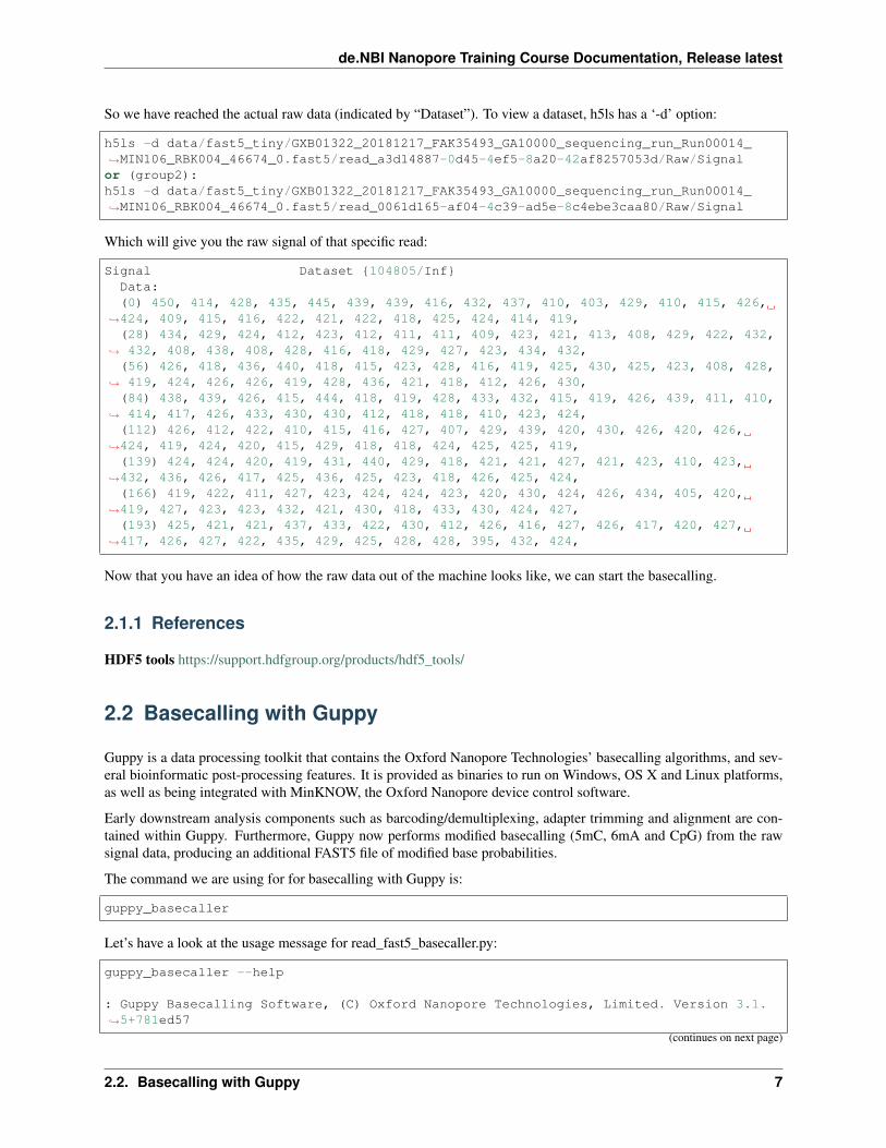
So we have reached the actual raw data (indicated by “Dataset”). To view a dataset, h5ls has a ‘-d’ option:
h5ls -d data/fast5_tiny/GXB01322_20181217_FAK35493_GA10000_sequencing_run_Run00014_→˓MIN106_RBK004_46674_0.fast5/read_a3d14887-0d45-4ef5-8a20-42af8257053d/Raw/Signalor (group2):h5ls -d data/fast5_tiny/GXB01322_20181217_FAK35493_GA10000_sequencing_run_Run00014_→˓MIN106_RBK004_46674_0.fast5/read_0061d165-af04-4c39-ad5e-8c4ebe3caa80/Raw/Signal
Which will give you the raw signal of that specific read:
Signal Dataset {104805/Inf}Data:(0) 450, 414, 428, 435, 445, 439, 439, 416, 432, 437, 410, 403, 429, 410, 415, 426,
→˓424, 409, 415, 416, 422, 421, 422, 418, 425, 424, 414, 419,(28) 434, 429, 424, 412, 423, 412, 411, 411, 409, 423, 421, 413, 408, 429, 422, 432,
→˓ 432, 408, 438, 408, 428, 416, 418, 429, 427, 423, 434, 432,(56) 426, 418, 436, 440, 418, 415, 423, 428, 416, 419, 425, 430, 425, 423, 408, 428,
→˓ 419, 424, 426, 426, 419, 428, 436, 421, 418, 412, 426, 430,(84) 438, 439, 426, 415, 444, 418, 419, 428, 433, 432, 415, 419, 426, 439, 411, 410,
→˓ 414, 417, 426, 433, 430, 430, 412, 418, 418, 410, 423, 424,(112) 426, 412, 422, 410, 415, 416, 427, 407, 429, 439, 420, 430, 426, 420, 426,
→˓424, 419, 424, 420, 415, 429, 418, 418, 424, 425, 425, 419,(139) 424, 424, 420, 419, 431, 440, 429, 418, 421, 421, 427, 421, 423, 410, 423,
→˓432, 436, 426, 417, 425, 436, 425, 423, 418, 426, 425, 424,(166) 419, 422, 411, 427, 423, 424, 424, 423, 420, 430, 424, 426, 434, 405, 420,
→˓419, 427, 423, 423, 432, 421, 430, 418, 433, 430, 424, 427,(193) 425, 421, 421, 437, 433, 422, 430, 412, 426, 416, 427, 426, 417, 420, 427,
→˓417, 426, 427, 422, 435, 429, 425, 428, 428, 395, 432, 424,
Now that you have an idea of how the raw data out of the machine looks like, we can start the basecalling.
2.1.1 References
HDF5 tools https://support.hdfgroup.org/products/hdf5_tools/
2.2 Basecalling with Guppy
Guppy is a data processing toolkit that contains the Oxford Nanopore Technologies’ basecalling algorithms, and sev-eral bioinformatic post-processing features. It is provided as binaries to run on Windows, OS X and Linux platforms,as well as being integrated with MinKNOW, the Oxford Nanopore device control software.
Early downstream analysis components such as barcoding/demultiplexing, adapter trimming and alignment are con-tained within Guppy. Furthermore, Guppy now performs modified basecalling (5mC, 6mA and CpG) from the rawsignal data, producing an additional FAST5 file of modified base probabilities.
The command we are using for for basecalling with Guppy is:
guppy_basecaller
Let’s have a look at the usage message for read_fast5_basecaller.py:
guppy_basecaller --help
: Guppy Basecalling Software, (C) Oxford Nanopore Technologies, Limited. Version 3.1.→˓5+781ed57
(continues on next page)
2.2. Basecalling with Guppy 7

de.NBI Nanopore Training Course Documentation, Release latest
(continued from previous page)
Usage:
With config file:guppy_basecaller -i <input path> -s <save path> -c <config file> [options]
With flowcell and kit name:guppy_basecaller -i <input path> -s <save path> --flowcell <flowcell name>--kit <kit name>
List supported flowcells and kits:guppy_basecaller --print_workflows
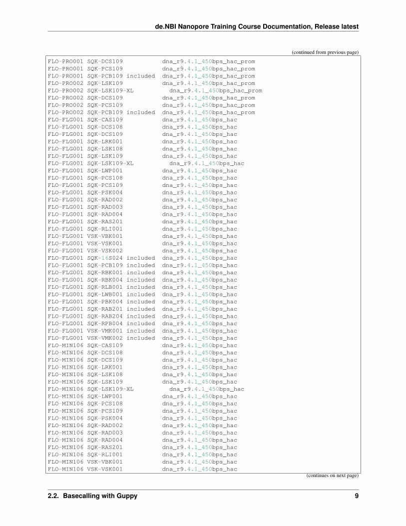
Beside the path of our fast5 files (-i), the basecaller requires an output path (-s) and a config file or the flowcell/kitcombination. In order to get a list of possible flowcell/kit combinations and config files, we use:
guppy_basecaller --print_workflows
Available flowcell + kit combinations are:flowcell kit barcoding config_nameFLO-MIN107 SQK-DCS108 dna_r9.5_450bpsFLO-MIN107 SQK-DCS109 dna_r9.5_450bpsFLO-MIN107 SQK-LRK001 dna_r9.5_450bpsFLO-MIN107 SQK-LSK108 dna_r9.5_450bpsFLO-MIN107 SQK-LSK109 dna_r9.5_450bpsFLO-MIN107 SQK-LSK308 dna_r9.5_450bpsFLO-MIN107 SQK-LSK309 dna_r9.5_450bpsFLO-MIN107 SQK-LSK319 dna_r9.5_450bpsFLO-MIN107 SQK-LWP001 dna_r9.5_450bpsFLO-MIN107 SQK-PCS108 dna_r9.5_450bpsFLO-MIN107 SQK-PCS109 dna_r9.5_450bpsFLO-MIN107 SQK-PSK004 dna_r9.5_450bpsFLO-MIN107 SQK-RAD002 dna_r9.5_450bpsFLO-MIN107 SQK-RAD003 dna_r9.5_450bpsFLO-MIN107 SQK-RAD004 dna_r9.5_450bpsFLO-MIN107 SQK-RAS201 dna_r9.5_450bpsFLO-MIN107 SQK-RLI001 dna_r9.5_450bpsFLO-MIN107 VSK-VBK001 dna_r9.5_450bpsFLO-MIN107 VSK-VSK001 dna_r9.5_450bpsFLO-MIN107 VSK-VSK002 dna_r9.5_450bpsFLO-MIN107 SQK-LWB001 included dna_r9.5_450bpsFLO-MIN107 SQK-PBK004 included dna_r9.5_450bpsFLO-MIN107 SQK-RAB201 included dna_r9.5_450bpsFLO-MIN107 SQK-RAB204 included dna_r9.5_450bpsFLO-MIN107 SQK-RBK001 included dna_r9.5_450bpsFLO-MIN107 SQK-RBK004 included dna_r9.5_450bpsFLO-MIN107 SQK-RLB001 included dna_r9.5_450bpsFLO-MIN107 SQK-RPB004 included dna_r9.5_450bpsFLO-MIN107 VSK-VMK001 included dna_r9.5_450bpsFLO-MIN107 VSK-VMK002 included dna_r9.5_450bpsFLO-FLG001 SQK-RNA001 rna_r9.4.1_70bps_hacFLO-FLG001 SQK-RNA002 rna_r9.4.1_70bps_hacFLO-MIN106 SQK-RNA001 rna_r9.4.1_70bps_hacFLO-MIN106 SQK-RNA002 rna_r9.4.1_70bps_hacFLO-MIN107 SQK-RNA001 rna_r9.4.1_70bps_hacFLO-MIN107 SQK-RNA002 rna_r9.4.1_70bps_hacFLO-PRO001 SQK-LSK109 dna_r9.4.1_450bps_hac_promFLO-PRO001 SQK-LSK109-XL dna_r9.4.1_450bps_hac_prom
(continues on next page)
8 Chapter 2. Basecalling
de.NBI Nanopore Training Course Documentation, Release latest
(continued from previous page)
FLO-PRO001 SQK-DCS109 dna_r9.4.1_450bps_hac_promFLO-PRO001 SQK-PCS109 dna_r9.4.1_450bps_hac_promFLO-PRO001 SQK-PCB109 included dna_r9.4.1_450bps_hac_promFLO-PRO002 SQK-LSK109 dna_r9.4.1_450bps_hac_promFLO-PRO002 SQK-LSK109-XL dna_r9.4.1_450bps_hac_promFLO-PRO002 SQK-DCS109 dna_r9.4.1_450bps_hac_promFLO-PRO002 SQK-PCS109 dna_r9.4.1_450bps_hac_promFLO-PRO002 SQK-PCB109 included dna_r9.4.1_450bps_hac_promFLO-FLG001 SQK-CAS109 dna_r9.4.1_450bps_hacFLO-FLG001 SQK-DCS108 dna_r9.4.1_450bps_hacFLO-FLG001 SQK-DCS109 dna_r9.4.1_450bps_hacFLO-FLG001 SQK-LRK001 dna_r9.4.1_450bps_hacFLO-FLG001 SQK-LSK108 dna_r9.4.1_450bps_hacFLO-FLG001 SQK-LSK109 dna_r9.4.1_450bps_hacFLO-FLG001 SQK-LSK109-XL dna_r9.4.1_450bps_hacFLO-FLG001 SQK-LWP001 dna_r9.4.1_450bps_hacFLO-FLG001 SQK-PCS108 dna_r9.4.1_450bps_hacFLO-FLG001 SQK-PCS109 dna_r9.4.1_450bps_hacFLO-FLG001 SQK-PSK004 dna_r9.4.1_450bps_hacFLO-FLG001 SQK-RAD002 dna_r9.4.1_450bps_hacFLO-FLG001 SQK-RAD003 dna_r9.4.1_450bps_hacFLO-FLG001 SQK-RAD004 dna_r9.4.1_450bps_hacFLO-FLG001 SQK-RAS201 dna_r9.4.1_450bps_hacFLO-FLG001 SQK-RLI001 dna_r9.4.1_450bps_hacFLO-FLG001 VSK-VBK001 dna_r9.4.1_450bps_hacFLO-FLG001 VSK-VSK001 dna_r9.4.1_450bps_hacFLO-FLG001 VSK-VSK002 dna_r9.4.1_450bps_hacFLO-FLG001 SQK-16S024 included dna_r9.4.1_450bps_hacFLO-FLG001 SQK-PCB109 included dna_r9.4.1_450bps_hacFLO-FLG001 SQK-RBK001 included dna_r9.4.1_450bps_hacFLO-FLG001 SQK-RBK004 included dna_r9.4.1_450bps_hacFLO-FLG001 SQK-RLB001 included dna_r9.4.1_450bps_hacFLO-FLG001 SQK-LWB001 included dna_r9.4.1_450bps_hacFLO-FLG001 SQK-PBK004 included dna_r9.4.1_450bps_hacFLO-FLG001 SQK-RAB201 included dna_r9.4.1_450bps_hacFLO-FLG001 SQK-RAB204 included dna_r9.4.1_450bps_hacFLO-FLG001 SQK-RPB004 included dna_r9.4.1_450bps_hacFLO-FLG001 VSK-VMK001 included dna_r9.4.1_450bps_hacFLO-FLG001 VSK-VMK002 included dna_r9.4.1_450bps_hacFLO-MIN106 SQK-CAS109 dna_r9.4.1_450bps_hacFLO-MIN106 SQK-DCS108 dna_r9.4.1_450bps_hacFLO-MIN106 SQK-DCS109 dna_r9.4.1_450bps_hacFLO-MIN106 SQK-LRK001 dna_r9.4.1_450bps_hacFLO-MIN106 SQK-LSK108 dna_r9.4.1_450bps_hacFLO-MIN106 SQK-LSK109 dna_r9.4.1_450bps_hacFLO-MIN106 SQK-LSK109-XL dna_r9.4.1_450bps_hacFLO-MIN106 SQK-LWP001 dna_r9.4.1_450bps_hacFLO-MIN106 SQK-PCS108 dna_r9.4.1_450bps_hacFLO-MIN106 SQK-PCS109 dna_r9.4.1_450bps_hacFLO-MIN106 SQK-PSK004 dna_r9.4.1_450bps_hacFLO-MIN106 SQK-RAD002 dna_r9.4.1_450bps_hacFLO-MIN106 SQK-RAD003 dna_r9.4.1_450bps_hacFLO-MIN106 SQK-RAD004 dna_r9.4.1_450bps_hacFLO-MIN106 SQK-RAS201 dna_r9.4.1_450bps_hacFLO-MIN106 SQK-RLI001 dna_r9.4.1_450bps_hacFLO-MIN106 VSK-VBK001 dna_r9.4.1_450bps_hacFLO-MIN106 VSK-VSK001 dna_r9.4.1_450bps_hac
(continues on next page)
2.2. Basecalling with Guppy 9

de.NBI Nanopore Training Course Documentation, Release latest
(continued from previous page)
FLO-MIN106 VSK-VSK002 dna_r9.4.1_450bps_hacFLO-MIN106 SQK-16S024 included dna_r9.4.1_450bps_hacFLO-MIN106 SQK-PCB109 included dna_r9.4.1_450bps_hacFLO-MIN106 SQK-RBK001 included dna_r9.4.1_450bps_hacFLO-MIN106 SQK-RBK004 included dna_r9.4.1_450bps_hacFLO-MIN106 SQK-RLB001 included dna_r9.4.1_450bps_hacFLO-MIN106 SQK-LWB001 included dna_r9.4.1_450bps_hacFLO-MIN106 SQK-PBK004 included dna_r9.4.1_450bps_hacFLO-MIN106 SQK-RAB201 included dna_r9.4.1_450bps_hacFLO-MIN106 SQK-RAB204 included dna_r9.4.1_450bps_hacFLO-MIN106 SQK-RPB004 included dna_r9.4.1_450bps_hacFLO-MIN106 VSK-VMK001 included dna_r9.4.1_450bps_hacFLO-MIN106 VSK-VMK002 included dna_r9.4.1_450bps_hacFLO-PRO001 SQK-RNA002 rna_r9.4.1_70bps_hac_promFLO-PRO002 SQK-RNA002 rna_r9.4.1_70bps_hac_prom
Our dataset was generated using the FLO-MIN106 flowcell, and the LSK109 kit, so we can use thedna_r9.4.1_450bps_hac model.
We need to specify the following options:
What? parameter Our valueThe config file for our flowcell/kit combination -c dna_r9.4.1_450bps_hac_model.cfgCompress the fastq output –compress_fastqThe full path to the directory where the raw read files arelocated
-i ~/workdir/data/fast5_small
The full path to the directory where the basecalled fileswill be saved
-s ~/workdir/basecall_small/
How many worker threads you are using –cpu_threads_per_caller14Number of parallel basecallers to create –num_callers 1
Our complete command line is:
guppy_basecaller --compress_fastq -i ~/workdir/data/fast5_tiny/ -s ~/workdir/basecall_→˓tiny/ --cpu_threads_per_caller 14 --num_callers 1 -c dna_r9.4.1_450bps_hac.cfg
2.2.1 References
guppy https://nanoporetech.com/
2.3 Inspect the output
The directory contains the following output:
ls -l ~/workdir/basecall_tiny/
total 4456-rw-rw-r-- 1 ubuntu ubuntu 3995875 Sep 18 09:56 fastq_runid_→˓b110eefd3ba5e91817c69585fcd2257218eeb796_0.fastq.gz-rw-rw-r-- 1 ubuntu ubuntu 261383 Sep 18 09:56 guppy_basecaller_log-2019-09-18_09-49-→˓20.log
(continues on next page)
10 Chapter 2. Basecalling
de.NBI Nanopore Training Course Documentation, Release latest
(continued from previous page)
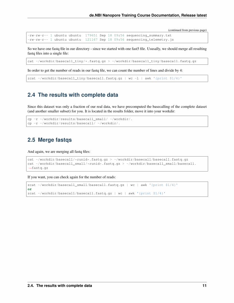
-rw-rw-r-- 1 ubuntu ubuntu 179651 Sep 18 09:56 sequencing_summary.txt-rw-rw-r-- 1 ubuntu ubuntu 121167 Sep 18 09:56 sequencing_telemetry.js
So we have one fastq file in our directory - since we started with one fast5 file. Ususally, we should merge all resultingfastq files into a single file:
cat ~/workdir/basecall_tiny/*.fastq.gz > ~/workdir/basecall_tiny/basecall.fastq.gz
In order to get the number of reads in our fastq file, we can count the number of lines and divide by 4:
zcat ~/workdir/basecall_tiny/basecall.fastq.gz | wc -l | awk '{print $1/4}'
2.4 The results with complete data
Since this dataset was only a fraction of our real data, we have precomputed the basecalling of the complete dataset(and another smaller subset) for you. It is located in the results folder, move it into your workdir:
cp -r ~/workdir/results/basecall_small/ ~/workdir/.cp -r ~/workdir/results/basecall/ ~/workdir/.
2.5 Merge fastqs
And again, we are merging all fastq files:
cat ~/workdir/basecall/*runid*.fastq.gz > ~/workdir/basecall/basecall.fastq.gzcat ~/workdir/basecall_small/*runid*.fastq.gz > ~/workdir/basecall_small/basecall.→˓fastq.gz
If you want, you can check again for the number of reads:
zcat ~/workdir/basecall_small/basecall.fastq.gz | wc | awk '{print $1/4}'orzcat ~/workdir/basecall/basecall.fastq.gz | wc | awk '{print $1/4}'
2.4. The results with complete data 11

de.NBI Nanopore Training Course Documentation, Release latest
12 Chapter 2. Basecalling

CHAPTER 3
Data Quality Assessment
In the following, we will assess the data quality by looking at the sequencing effort, the raw reads and the data qualityas reported by the sequencing instrument (using MinIONQC and FastQC) as well as inferring the actual data qualityby aligning the reads to the reference genome (read mapping).
3.1 MinIONQC
Developed by Rob Lanfear:
R Lanfear, M Schalamun, D Kainer, W Wang, B Schwessinger; MinIONQC: fast and simple→˓quality control for MinION sequencing data, Bioinformatics, , bty654, https://doi.→˓org/10.1093/bioinformatics/bty654
Script collection that will generate a range of diagnostic plots for quality control of sequencing data from OxfordNanopore’s MinION sequencer.
MinIONQC works directly with the sequencing_summary.txt files produced by ONT’s Albacore or Guppy base callers.This allows MinIONQC for quick-and-easy comparison of data from one or multiple flowcells.
Complete manual can be looked up at: https://github.com/roblanf/minion_qc
Usage:
Rscript ~/MinIONQC.R --helpUsage: /home/ubuntu/MinIONQC.R [options]
Options:
-h, --help Show this help message and exit
-i INPUT, --input=INPUT Input file or directory (required). Either a full path to a se-quence_summary.txt file, or a full path to a directory containing one ormore such files. In the latter case the directory is searched recursively.
13
de.NBI Nanopore Training Course Documentation, Release latest
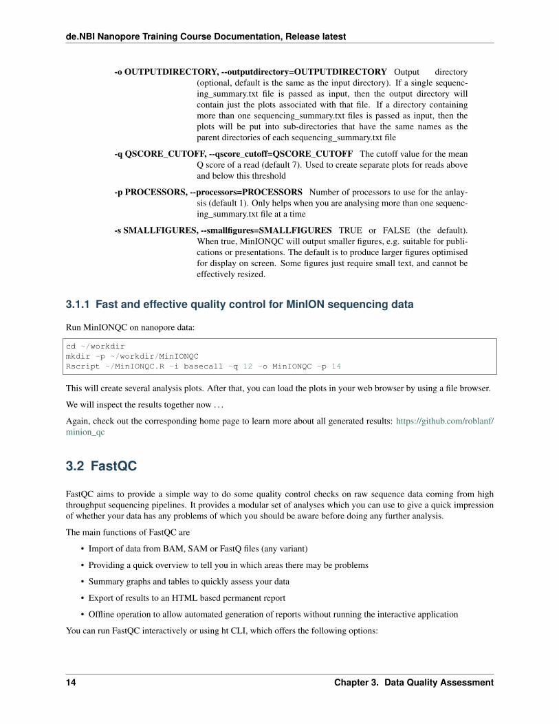
-o OUTPUTDIRECTORY, --outputdirectory=OUTPUTDIRECTORY Output directory(optional, default is the same as the input directory). If a single sequenc-ing_summary.txt file is passed as input, then the output directory willcontain just the plots associated with that file. If a directory containingmore than one sequencing_summary.txt files is passed as input, then theplots will be put into sub-directories that have the same names as theparent directories of each sequencing_summary.txt file
-q QSCORE_CUTOFF, --qscore_cutoff=QSCORE_CUTOFF The cutoff value for the meanQ score of a read (default 7). Used to create separate plots for reads aboveand below this threshold
-p PROCESSORS, --processors=PROCESSORS Number of processors to use for the anlay-sis (default 1). Only helps when you are analysing more than one sequenc-ing_summary.txt file at a time
-s SMALLFIGURES, --smallfigures=SMALLFIGURES TRUE or FALSE (the default).When true, MinIONQC will output smaller figures, e.g. suitable for publi-cations or presentations. The default is to produce larger figures optimisedfor display on screen. Some figures just require small text, and cannot beeffectively resized.
3.1.1 Fast and effective quality control for MinION sequencing data
Run MinIONQC on nanopore data:
cd ~/workdirmkdir -p ~/workdir/MinIONQCRscript ~/MinIONQC.R -i basecall -q 12 -o MinIONQC -p 14
This will create several analysis plots. After that, you can load the plots in your web browser by using a file browser.
We will inspect the results together now . . .
Again, check out the corresponding home page to learn more about all generated results: https://github.com/roblanf/minion_qc
3.2 FastQC
FastQC aims to provide a simple way to do some quality control checks on raw sequence data coming from highthroughput sequencing pipelines. It provides a modular set of analyses which you can use to give a quick impressionof whether your data has any problems of which you should be aware before doing any further analysis.
The main functions of FastQC are
• Import of data from BAM, SAM or FastQ files (any variant)
• Providing a quick overview to tell you in which areas there may be problems
• Summary graphs and tables to quickly assess your data
• Export of results to an HTML based permanent report
• Offline operation to allow automated generation of reports without running the interactive application
You can run FastQC interactively or using ht CLI, which offers the following options:
14 Chapter 3. Data Quality Assessment

de.NBI Nanopore Training Course Documentation, Release latest
fastqc --help
SYNOPSIS
fastqc seqfile1 seqfile2 .. seqfileN
fastqc [-o output dir] [--(no)extract] [-f fastq|bam|sam] [-c contaminant file]→˓seqfile1 .. seqfileN
OPTIONS:
-o --outdir Create all output files in the specified output directory.Please note that this directory must exist as the programwill not create it. If this option is not set then theoutput file for each sequence file is created in the samedirectory as the sequence file which was processed.
--casava Files come from raw casava output. Files in the same samplegroup (differing only by the group number) will be analysedas a set rather than individually. Sequences with the filterflag set in the header will be excluded from the analysis.Files must have the same names given to them by casava(including being gzipped and ending with .gz) otherwise theywon't be grouped together correctly.
--nano Files come from naopore sequences and are in fast5 format. Inthis mode you can pass in directories to process and the programwill take in all fast5 files within those directories and producea single output file from the sequences found in all files.
--nofilter If running with --casava then don't remove read flagged bycasava as poor quality when performing the QC analysis.
--nogroup Disable grouping of bases for reads >50bp. All reports willshow data for every base in the read. WARNING: Using thisoption will cause fastqc to crash and burn if you use it onreally long reads, and your plots may end up a ridiculous size.You have been warned!
-f --format Bypasses the normal sequence file format detection andforces the program to use the specified format. Validformats are bam,sam,bam_mapped,sam_mapped and fastq
-t --threads Specifies the number of files which can be processedsimultaneously. Each thread will be allocated 250MB ofmemory so you shouldn't run more threads than youravailable memory will cope with, and not more than6 threads on a 32 bit machine
-c Specifies a non-default file which contains the list of--contaminants contaminants to screen overrepresented sequences against.
The file must contain sets of named contaminants in theform name[tab]sequence. Lines prefixed with a hash willbe ignored.
-a Specifies a non-default file which contains the list of--adapters adapter sequences which will be explicity searched against
(continues on next page)
3.2. FastQC 15

de.NBI Nanopore Training Course Documentation, Release latest
(continued from previous page)
the library. The file must contain sets of named adaptersin the form name[tab]sequence. Lines prefixed with a hashwill be ignored.
-l Specifies a non-default file which contains a set of criteria--limits which will be used to determine the warn/error limits for the
various modules. This file can also be used to selectivelyremove some modules from the output all together. The formatneeds to mirror the default limits.txt file found in theConfiguration folder.
-k --kmers Specifies the length of Kmer to look for in the Kmer contentmodule. Specified Kmer length must be between 2 and 10. Defaultlength is 7 if not specified.
-q --quiet Supress all progress messages on stdout and only report errors.
-d --dir Selects a directory to be used for temporary files written whengenerating report images. Defaults to system temp directory ifnot specified.
See the FastQC home page for more info.
3.2.1 QA with FastQC
Evaluate with fastqc:
cd ~/workdirmkdir -p ~/workdir/fastqc/nanopore_fastqcmkdir -p ~/workdir/fastqc/illumina_fastqcfastqc -t 14 -o ~/workdir/fastqc/nanopore_fastqc ~/workdir/basecall/basecall.fastq.gzfastqc -t 14 -o ~/workdir/fastqc/illumina_fastqc ~/workdir/data/illumina/Illumina_R1.→˓fastq.gz ~/workdir/data/illumina/Illumina_R2.fastq.gz
After that, you can load the reports in your web browser. Open a file browser, go to your workdir/fastqc/ directory anddouble click the html file.
We will inspect the results together now . . .
You should also check out the FastQC home page for examples of reports including bad data.
3.2.2 Handle adapter contamination
As we see some strange GC content at the 5’ end of our nanopore reads, we can alter the way the plots are generatedand turn off the grouping of reads into bins. Notice, this will generate very huge plots! To avoid this, we will first trimour reads to the first 100 base positions and do the analysis only on that:
cd ~/workdirmkdir -p ~/workdir/fastqc/nanopore_fastqc_nogroupzcat ~/workdir/basecall/basecall.fastq.gz | perl -ne '{chomp; if ($.%2) {print $_."\n→˓"} else {print substr($_,0,100)."\n"} }' | gzip > ~/workdir/basecall/basecall_100.→˓fastq.gzfastqc -t 14 -o ~/workdir/fastqc/nanopore_fastqc_nogroup --nogroup --extract ~/→˓workdir/basecall/basecall_100.fastq.gzgrep -A 100 "Per base sequence" ~/workdir/fastqc/nanopore_fastqc_nogroup/basecall_100_→˓fastqc/fastqc_data.txt (continues on next page)
16 Chapter 3. Data Quality Assessment

de.NBI Nanopore Training Course Documentation, Release latest
(continued from previous page)
So the first bases may indicate an adaptor contamination. For workflows including de novo assembly refined withnanopolish or medaka adaptor trimming is not necessary, but in other workflow scenarios this can be important to doand good there are tools which can handle this, as e.g. porechop.
Porechop is a tool for finding and removing adapters from Oxford Nanopore reads. Adapters on the ends of reads aretrimmed off, and when a read has an adapter in its middle, it is treated as chimeric and chopped into separate reads.Porechop performs thorough alignments to effectively find adapters, even at low sequence identity:
cd ~/workdirporechop -i ~/workdir/basecall/basecall.fastq.gz -t 14 -v 2 -o ~/workdir/basecall/→˓basecall_trimmed.fastq.gz > porechop.log
Let’s inspect the log file:
more porechop.log
So here, the following adapters were found and trimmed:
Trimming adapters from read endsRapid_adapter: GTTTTCGCATTTATCGTGAAACGCTTTCGCGTTTTTCGTGCGCCGCTTCA
BC04_rev: TAGGGAAACACGATAGAATCCGAABC04: TTCGGATTCTATCGTGTTTCCCTA
BC11_rev: TCCATTCCCTCCGATAGATGAAACBC11: GTTTCATCTATCGGAGGGAATGGABC06: TTCTCGCAAAGGCAGAAAGTAGTC
BC06_rev: GACTACTTTCTGCCTTTGCGAGAA
To see how many reads were trimmed, grep for reads:
grep reads porechop.log
52,536 reads loaded51,299 / 52,536 reads had adapters trimmed from their start (5,257,865 bp removed)4,890 / 52,536 reads had adapters trimmed from their end (47,632 bp removed)794 / 52,536 reads were split based on middle adapters
We will again look into the results of FastQC:
mkdir -p ~/workdir/fastqc/nanopore_fastqc_trimmed/fastqc -t 14 -o ~/workdir/fastqc/nanopore_fastqc_trimmed/ ~/workdir/basecall/→˓basecall_trimmed.fastq.gz
3.2.3 References
FastQC https://www.bioinformatics.babraham.ac.uk/projects/fastqc/
Porechop https://github.com/rrwick/Porechop
3.2. FastQC 17
de.NBI Nanopore Training Course Documentation, Release latest
3.3 Generating Error Profiles
3.3.1 Mapping the data
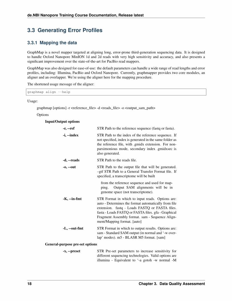
GraphMap is a novel mapper targeted at aligning long, error-prone third-generation sequencing data. It is designedto handle Oxford Nanopore MinION 1d and 2d reads with very high sensitivity and accuracy, and also presents asignificant improvement over the state-of-the-art for PacBio read mappers.
GraphMap was also designed for ease-of-use: the default parameters can handle a wide range of read lengths and errorprofiles, including: Illumina, PacBio and Oxford Nanopore. Currently, graphmapper provides two core modules, analigner and an overlapper. We’re using the aligner here for the mapping procedure.
The shortened usage message of the aligner:
graphmap align --help
Usage:
graphmap [options] -r <reference_file> -d <reads_file> -o <output_sam_path>
Options
Input/Output options
-r, --ref STR Path to the reference sequence (fastq or fasta).
-i, --index STR Path to the index of the reference sequence. Ifnot specified, index is generated in the same folder asthe reference file, with .gmidx extension. For non-parsimonious mode, secondary index .gmidxsec isalso generated.
-d, --reads STR Path to the reads file.
-o, --out STR Path to the output file that will be generated.–gtf STR Path to a General Transfer Format file. Ifspecified, a transcriptome will be built
from the reference sequence and used for map-ping. Output SAM alignments will be ingenome space (not transcriptome).
-K, --in-fmt STR Format in which to input reads. Options are:auto - Determines the format automatically from fileextension. fastq - Loads FASTQ or FASTA files.fasta - Loads FASTQ or FASTA files. gfa - GraphicalFragment Assembly format. sam - Sequence Align-ment/Mapping format. [auto]
-L, --out-fmt STR Format in which to output results. Options are:sam - Standard SAM output (in normal and ‘-w over-lap’ modes). m5 - BLASR M5 format. [sam]
General-purpose pre-set options
-x, --preset STR Pre-set parameters to increase sensitivity fordifferent sequencing technologies. Valid options areillumina - Equivalent to ‘-a gotoh -w normal -M
18 Chapter 3. Data Quality Assessment
de.NBI Nanopore Training Course Documentation, Release latest
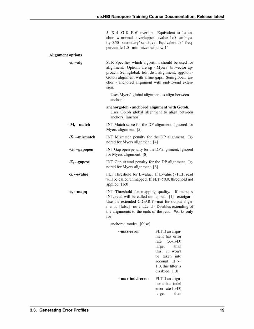
5 -X 4 -G 8 -E 6’ overlap - Equivalent to ‘-a an-chor -w normal –overlapper –evalue 1e0 –ambigu-ity 0.50 –secondary’ sensitive - Equivalent to ‘–freq-percentile 1.0 –minimizer-window 1’
Alignment options
-a, --alg STR Specifies which algorithm should be used foralignment. Options are sg - Myers’ bit-vector ap-proach. Semiglobal. Edit dist. alignment. sggotoh -Gotoh alignment with affine gaps. Semiglobal. an-chor - anchored alignment with end-to-end exten-sion.
Uses Myers’ global alignment to align betweenanchors.
anchorgotoh - anchored alignment with Gotoh.Uses Gotoh global alignment to align betweenanchors. [anchor]
-M, --match INT Match score for the DP alignment. Ignored forMyers alignment. [5]
-X, --mismatch INT Mismatch penalty for the DP alignment. Ig-nored for Myers alignment. [4]
-G, --gapopen INT Gap open penalty for the DP alignment. Ignoredfor Myers alignment. [8]
-E, --gapext INT Gap extend penalty for the DP alignment. Ig-nored for Myers alignment. [6]
-z, --evalue FLT Threshold for E-value. If E-value > FLT, readwill be called unmapped. If FLT < 0.0, thredhold notapplied. [1e0]
-c, --mapq INT Threshold for mapping quality. If mapq <INT, read will be called unmapped. [1] –extcigar -Use the extended CIGAR format for output align-ments. [false] –no-end2end - Disables extending ofthe alignments to the ends of the read. Works onlyfor
anchored modes. [false]
--max-error FLT If an align-ment has errorrate (X+I+D)larger thanthis, it won’tbe taken intoaccount. If >=1.0, this filter isdisabled. [1.0]
--max-indel-error FLT If an align-ment has indelerror rate (I+D)larger than
3.3. Generating Error Profiles 19
de.NBI Nanopore Training Course Documentation, Release latest
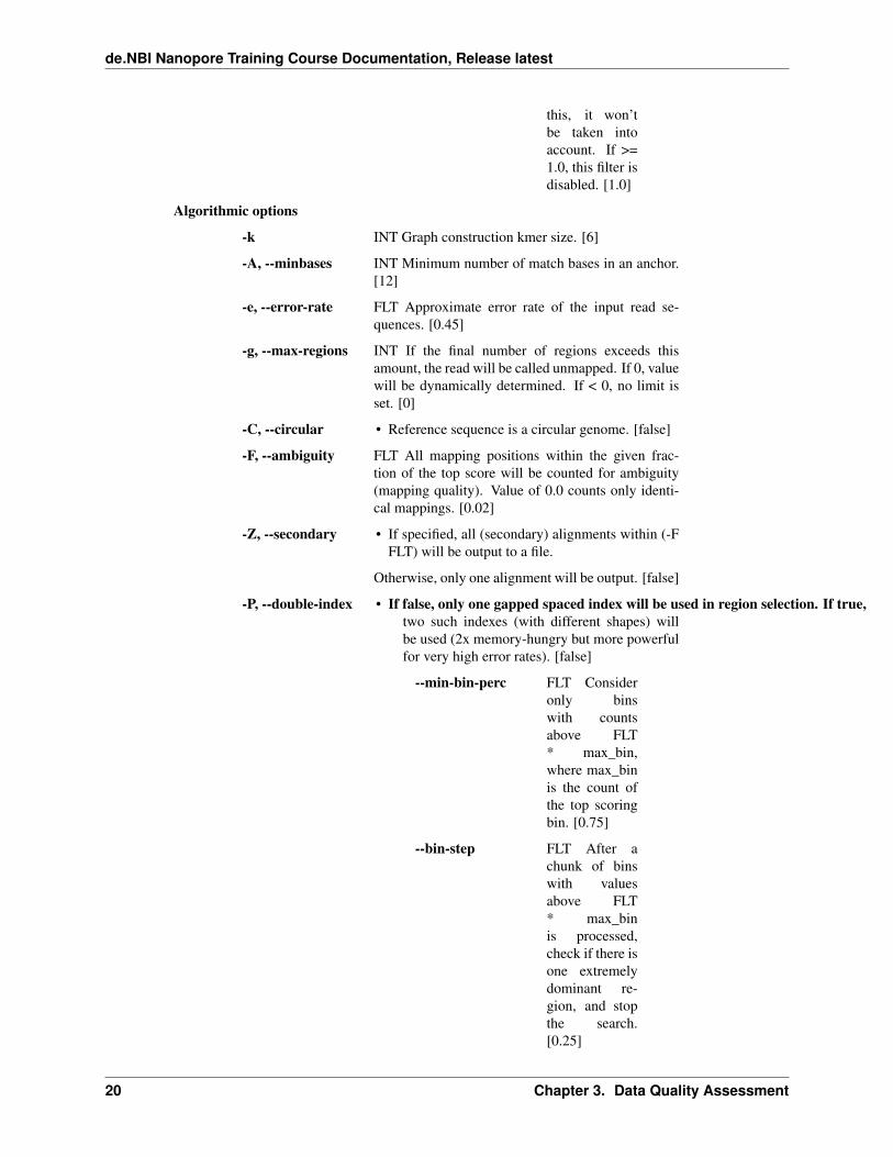
this, it won’tbe taken intoaccount. If >=1.0, this filter isdisabled. [1.0]
Algorithmic options
-k INT Graph construction kmer size. [6]
-A, --minbases INT Minimum number of match bases in an anchor.[12]
-e, --error-rate FLT Approximate error rate of the input read se-quences. [0.45]
-g, --max-regions INT If the final number of regions exceeds thisamount, the read will be called unmapped. If 0, valuewill be dynamically determined. If < 0, no limit isset. [0]
-C, --circular • Reference sequence is a circular genome. [false]
-F, --ambiguity FLT All mapping positions within the given frac-tion of the top score will be counted for ambiguity(mapping quality). Value of 0.0 counts only identi-cal mappings. [0.02]
-Z, --secondary • If specified, all (secondary) alignments within (-FFLT) will be output to a file.
Otherwise, only one alignment will be output. [false]
-P, --double-index • If false, only one gapped spaced index will be used in region selection. If true,two such indexes (with different shapes) willbe used (2x memory-hungry but more powerfulfor very high error rates). [false]
--min-bin-perc FLT Consideronly binswith countsabove FLT* max_bin,where max_binis the count ofthe top scoringbin. [0.75]
--bin-step FLT After achunk of binswith valuesabove FLT* max_binis processed,check if there isone extremelydominant re-gion, and stopthe search.[0.25]
20 Chapter 3. Data Quality Assessment

de.NBI Nanopore Training Course Documentation, Release latest
--min-read-len INT If a readis shorter thanthis, it willbe marked asunmapped.This value canbe lowered ifthe reads areknown to beaccurate. [80]
--minimizer-window INT Length ofthe window toselect a mini-mizer from. Ifequal to 1, min-imizers will beturned off. [5]
--freq-percentile FLT Filer the(1.0 - value)percent of mostfrequent seedsin the lookupprocess. [0.99]
--fly-index • Index will beconstructedon the fly,without stor-ing it to disk.If it already
exists on disk,it will beloaded unless–rebuild-indexis specified.[false]
Other options
-t, --threads INT Number of threads to use. If ‘-1’, number ofthreads will be equal to min(24, num_cores/2). [-1]
-v, --verbose INT Verbose level. If equal to 0 nothing except strictoutput will be placed on stdout. [5]
-h, --help • View this help. [false]
We now use graphmap to align the different read sets to the reference, starting with the nanopore reads:
cd ~/workdirmkdir ~/workdir/map_to_refgraphmap align -r ~/workdir/data/Reference.fna -t 14 -C -d ~/workdir/basecall/→˓basecall.fastq.gz -o ~/workdir/map_to_ref/nanopore.graphmap.sam > ~/workdir/map_to_→˓ref/nanopore.graphmap.sam.log 2>&1
3.3. Generating Error Profiles 21
de.NBI Nanopore Training Course Documentation, Release latest
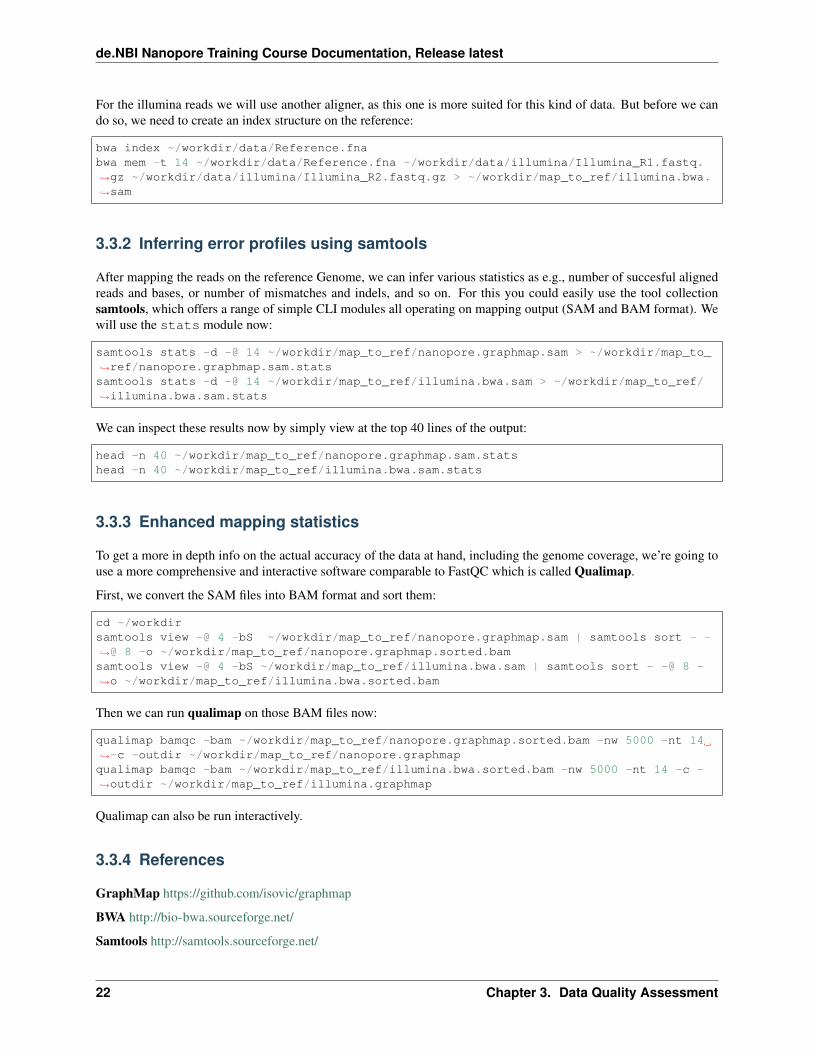
For the illumina reads we will use another aligner, as this one is more suited for this kind of data. But before we cando so, we need to create an index structure on the reference:
bwa index ~/workdir/data/Reference.fnabwa mem -t 14 ~/workdir/data/Reference.fna ~/workdir/data/illumina/Illumina_R1.fastq.→˓gz ~/workdir/data/illumina/Illumina_R2.fastq.gz > ~/workdir/map_to_ref/illumina.bwa.→˓sam
3.3.2 Inferring error profiles using samtools
After mapping the reads on the reference Genome, we can infer various statistics as e.g., number of succesful alignedreads and bases, or number of mismatches and indels, and so on. For this you could easily use the tool collectionsamtools, which offers a range of simple CLI modules all operating on mapping output (SAM and BAM format). Wewill use the stats module now:
samtools stats -d -@ 14 ~/workdir/map_to_ref/nanopore.graphmap.sam > ~/workdir/map_to_→˓ref/nanopore.graphmap.sam.statssamtools stats -d -@ 14 ~/workdir/map_to_ref/illumina.bwa.sam > ~/workdir/map_to_ref/→˓illumina.bwa.sam.stats
We can inspect these results now by simply view at the top 40 lines of the output:
head -n 40 ~/workdir/map_to_ref/nanopore.graphmap.sam.statshead -n 40 ~/workdir/map_to_ref/illumina.bwa.sam.stats
3.3.3 Enhanced mapping statistics
To get a more in depth info on the actual accuracy of the data at hand, including the genome coverage, we’re going touse a more comprehensive and interactive software comparable to FastQC which is called Qualimap.
First, we convert the SAM files into BAM format and sort them:
cd ~/workdirsamtools view -@ 4 -bS ~/workdir/map_to_ref/nanopore.graphmap.sam | samtools sort - -→˓@ 8 -o ~/workdir/map_to_ref/nanopore.graphmap.sorted.bamsamtools view -@ 4 -bS ~/workdir/map_to_ref/illumina.bwa.sam | samtools sort - -@ 8 -→˓o ~/workdir/map_to_ref/illumina.bwa.sorted.bam
Then we can run qualimap on those BAM files now:
qualimap bamqc -bam ~/workdir/map_to_ref/nanopore.graphmap.sorted.bam -nw 5000 -nt 14→˓-c -outdir ~/workdir/map_to_ref/nanopore.graphmapqualimap bamqc -bam ~/workdir/map_to_ref/illumina.bwa.sorted.bam -nw 5000 -nt 14 -c -→˓outdir ~/workdir/map_to_ref/illumina.graphmap
Qualimap can also be run interactively.
3.3.4 References
GraphMap https://github.com/isovic/graphmap
BWA http://bio-bwa.sourceforge.net/
Samtools http://samtools.sourceforge.net/
22 Chapter 3. Data Quality Assessment

de.NBI Nanopore Training Course Documentation, Release latest
QualiMap http://qualimap.bioinfo.cipf.es/doc_html/index.html
3.3. Generating Error Profiles 23

de.NBI Nanopore Training Course Documentation, Release latest
24 Chapter 3. Data Quality Assessment
CHAPTER 4
Assembly
We are going to create an assembly with canu and evaluate it with a mapping to the reference genome and with quast.
4.1 Assembly with canu
Canu is a fork of the Celera Assembler, designed for high-noise single-molecule sequencing (such as the PacBio RSII/Sequel or Oxford Nanopore MinION). Documentation can be found here: http://canu.readthedocs.io/en/latest/
Canu is a hierarchical assembly pipeline which runs in four steps: - Detect overlaps in high-noise sequences usingMHAP - Generate corrected sequence consensus - Trim corrected sequences - Assemble trimmed corrected sequences
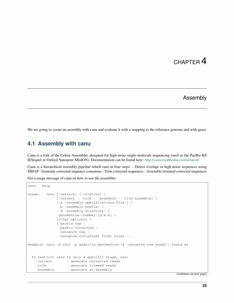
Get a usage message of canu on how to use the assembler:
canu --help
usage: canu [-version] [-citation] \[-correct | -trim | -assemble | -trim-assemble] \[-s <assembly-specifications-file>] \-p <assembly-prefix> \-d <assembly-directory> \genomeSize=<number>[g|m|k] \
[other-options] \[-pacbio-raw |-pacbio-corrected |-nanopore-raw |-nanopore-corrected] file1 file2 ...
example: canu -d run1 -p godzilla genomeSize=1g -nanopore-raw reads/*.fasta.gz
To restrict canu to only a specific stage, use:-correct - generate corrected reads-trim - generate trimmed reads-assemble - generate an assembly
(continues on next page)
25

de.NBI Nanopore Training Course Documentation, Release latest
(continued from previous page)
-trim-assemble - generate trimmed reads and then assemble them
The assembly is computed in the -d <assembly-directory>, with output files namedusing the -p <assembly-prefix>. This directory is created if needed. It is notpossible to run multiple assemblies in the same directory.
The genome size should be your best guess of the haploid genome size of what is→˓beingassembled. It is used primarily to estimate coverage in reads, NOT as the desiredassembly size. Fractional values are allowed: '4.7m' equals '4700k' equals '4700000
→˓'
Some common options:useGrid=string
- Run under grid control (true), locally (false), or set up for grid controlbut don't submit any jobs (remote)
rawErrorRate=fraction-error- The allowed difference in an overlap between two raw uncorrected reads. For
→˓lowerquality reads, use a higher number. The defaults are 0.300 for PacBio reads
→˓and0.500 for Nanopore reads.
correctedErrorRate=fraction-error- The allowed difference in an overlap between two corrected reads. Assemblies
→˓oflow coverage or data with biological differences will benefit from a slight
→˓increasein this. Defaults are 0.045 for PacBio reads and 0.144 for Nanopore reads.
gridOptions=string- Pass string to the command used to submit jobs to the grid. Can be used to
→˓setmaximum run time limits. Should NOT be used to set memory limits; Canu will
→˓dothat for you.
minReadLength=number- Ignore reads shorter than 'number' bases long. Default: 1000.
minOverlapLength=number- Ignore read-to-read overlaps shorter than 'number' bases long. Default: 500.
A full list of options can be printed with '-options'. All options can be supplied→˓inan optional sepc file with the -s option.
Reads can be either FASTA or FASTQ format, uncompressed, or compressed with gz, bz2→˓or xz.Reads are specified by the technology they were generated with:-pacbio-raw <files>-pacbio-corrected <files>-nanopore-raw <files>-nanopore-corrected <files>
We will run the assembly on the small dataset, to save time. The assembly for the complete dataset will take about onehour. We will perform the assembly in two steps:
Error correction with the parameter:
-correct - generate corrected reads
followed by trimming and assembly with the following parameters:
26 Chapter 4. Assembly

de.NBI Nanopore Training Course Documentation, Release latest
-trim-assemble - generate trimmed reads and then assemble them
You could also run the assembly completely in one step by leaving out both of these parameters. Running it in twosteps has the advantage, that both steps can be tested individually for good parameters without running both each timeagain.
4.1.1 Generate corrected reads
The correction stage selects the best overlaps to use for correction, estimates corrected read lengths, and generatescorrected reads:
canu -correct -d ~/workdir/correct_small -p assembly genomeSize=3m useGrid=false -→˓nanopore-raw ~/workdir/basecall_small/basecall.fastq.gz
It is also possible to run multiple correction rounds to eliminate errors. This has been done on a S. cerevisae dataset inthe canu publication. We will not do this in this course due to time limitations, but a script to do this, would look likethis:
COUNT=0NAME=input.fastafor i in `seq 1 10`; docanu -correct -p asm -d round$i \corOutCoverage=500 corMinCoverage=0 corMhapSensitivity=high \genomeSize=12.1m -nanopore-raw $NAMENAME="round$i/asm.correctedReads.fasta.gz"COUNT=`expr $COUNT + 1`donecanu -p asm -d asm genomeSize=12.1m -nanopore-corrected $NAME utgGraphDeviation=50
batOptions=”-ca 500 -cp 50”done
4.1.2 Generate and assemble trimmed reads
The trimming stage identifies unsupported regions in the input and trims or splits reads to their longest supportedrange. The assembly stage makes a final pass to identify sequencing errors; constructs the best overlap graph (BOG);and outputs contigs, an assembly graph, and summary statistics:
canu -trim-assemble -d ~/workdir/assembly_small -p assembly genomeSize=2M→˓useGrid=false -nanopore-corrected ~/workdir/correct_small/assembly.correctedReads.→˓fasta.gz
After that is done, inspect the results. We can get a quick view on the number of generated contigs with:
grep '>' ~/workdir/assembly_small/assembly.contigs.fasta
If there is time, we start the actual assembly with all data now:
Group 1:canu -d ~/workdir/assembly -p assembly "genomeSize=4.3M" useGrid=false -nanopore-raw ~→˓/workdir/basecall/basecall_trimmed.fastq.gzGroup 2:canu -d ~/workdir/assembly -p assembly "genomeSize=6.8M" useGrid=false -nanopore-raw ~→˓/workdir/basecall/basecall_trimmed.fastq.gz
4.1. Assembly with canu 27

de.NBI Nanopore Training Course Documentation, Release latest
Otherwise, copy the precomputed assembly with the complete dataset into your working directory:
cp -r ~/workdir/results/assembly/ ~/workdir/
and have a quick look on the number of contigs:
grep '>' ~/workdir/assembly/assembly.contigs.fasta
References
Canu https://github.com/marbl/canu
4.2 Assembly evaluation with QUAST
QUAST stands for QUality ASsessment Tool. The tool evaluates genome assemblies by computing various metrics.You can find all project news and the latest version of the tool at sourceforge. QUAST utilizes MUMmer, GeneMarkS,GeneMark-ES, GlimmerHMM, and GAGE.
To call quast.py we have to provide a reference genome and one or more assemblies. We are giving both, ourassembly with the reduced dataset as well as our assembly with the complete dataset as input. For comparison, wealso include an Illumina assembly which has been precomputed with spades. The reference is usually not available, ofcourse:
quast.py -t 14 -o ~/workdir/quast_canu_assembly -R ~/workdir/data/Reference.fna ~/→˓workdir/assembly/assembly.contigs.fasta ~/workdir/results/assembly_untrimmed/→˓assembly.contigs.fasta ~/workdir/assembly_small/assembly.contigs.fasta ~/workdir/→˓results/illumina_assembly/contigs.fasta
QUAST generates HTML reports including a number of interactive graphics. To access these reports, open them usinga file browser.
4.2.1 References
quast http://sourceforge.net/projects/quast
4.3 Assembly Graph inspection with bandage
Bandage is a program for visualising de novo assembly graphs. By displaying connections which are not present inthe contigs file, Bandage opens up new possibilities for analysing de novo assemblies.
You can start Bandage with:
Bandage
and load the following file:
~/workdir/assembly/assembly.contigs.gfa
and click on “Draw Graph” This is the assembly graph of our Nanopore Assembly. You can BLAST your contigs vseach other to identify further assembly problems by clicking “Create/View BLAST search”.
Compare this graph to a graph computed with Illumina data:
28 Chapter 4. Assembly

de.NBI Nanopore Training Course Documentation, Release latest
~/workdir/assembly/assembly_graph_with_scaffolds.gfa
4.3.1 References
Bandage https://rrwick.github.io/Bandage/
4.4 Quality control by mapping
In this part of the tutorial we will look at the assemblies by mapping the contigs of our first assembly to the referencegenome using LAST.
LAST is designed for comparing large datasets to each other (e.g. vertebrate genomes and/or large numbers of DNAreads). It can:
• Indicate the (un)ambiguity of each column in an alignment.
• Use sequence quality data in a rigorous fashion.
• Align DNA to proteins with frameshifts.
• Compare PSSMs to sequences.
• Calculate the likelihood of chance similarities between random sequences.
• Do split and spliced alignment.
• Train alignment parameters for unusual kinds of sequence (e.g. nanopore).
See the LAST webpage for more details.
LAST needs to build an index for the reference before we can align our assembly to it. This is done by the using thecommand lastdb:
cd ~/workdir/mkdir last_1st_assemblycd last_1st_assemblylastdb Reference.db ~/workdir/data/Reference.fna
Now that we have an index, we can map the assembly to the reference:
lastal Reference.db ~/workdir/assembly/assembly.contigs.fasta > canu_1st_Assembly.maf
lastal produces output in MAF format by default. As we are going to inspect the alignment in a genome viewer,we have to convert this into a sorted BAM file. LAST provides the script maf-convert to convert MAF to differentother formats:
maf-convert sam canu_1st_Assembly.maf > canu_1st_Assembly.sam
SAM and BAM files can be viewed and manipulated with SAMtools. Let’s first build an index for the FASTA file ofthe reference sequence:
samtools faidx ~/workdir/data/Reference.fna
Now we can convert the SAM file into the binary BAM format and add an appropriate header to the BAM file. Afterthat we need to sort the alignments in the BAM file by starting position (samtools sort) and index the file for fastaccess (samtools index):
4.4. Quality control by mapping 29

de.NBI Nanopore Training Course Documentation, Release latest
samtools view -bT ~/workdir/data/Reference.fna canu_1st_Assembly.sam > canu_1st_→˓Assembly.bamsamtools sort -o canu_1st_Assembly_sorted.bam canu_1st_Assembly.bamsamtools index canu_1st_Assembly_sorted.bam
To look at the BAM file use:
samtools view canu_1st_Assembly_sorted.bam | less
We will use a genome browser to look at the mappings. For this, you have to change java version to java 8:
sudo update-alternatives --config java
Choose java 8. Then start IGV:
igv
Now let’s look at the mapped contigs:
1. Load the reference genome into IGV. Use the menu Genomes->Load Genome from File...
2. Load the BAM file into IGV. Use menu File->Load from File...
Change java version back to Java 11:
sudo update-alternatives --config java
4.4.1 References
LAST http://last.cbrc.jp/
samtools http://www.htslib.org
IGV http://www.broadinstitute.org/igv/
30 Chapter 4. Assembly

CHAPTER 5
Assembly polishing
We are going to do 2 polishings to optimize our assembly: 1. Polishing with pilon using Illumina data 2. Polishingwith racon and medaka using Nanopore data
If there is time we are also going to polish the racon/medaka polished assembly with Pilon and Illumina data.
A possible polishing with nanopolish is also included in this docs, but we are not going to use it in this course.
5.1 Assembly polishing with pilon
Pilon is a software tool which can be used to automatically improve draft assemblies or to find variation among strains,including large event detection. Pilon requires as input a FASTA file of the genome along with one or more BAM filesof reads aligned to the input FASTA file. Pilon uses read alignment analysis to identify inconsistencies between theinput genome and the evidence in the reads. It then attempts to make improvements to the input genome, including:
• Single base differences
• Small indels
• Larger indel or block substitution events
• Gap filling
• Identification of local misassemblies, including optional opening of new gaps
Pilon then outputs a FASTA file containing an improved representation of the genome from the read data and anoptional VCF file detailing variation seen between the read data and the input genome.
To aid manual inspection and improvement by an analyst, Pilon can optionally produce tracks that can be displayedin genome viewers such as IGV and GenomeView, and it reports other events (such as possible large collapsed repeatregions) in its standard output. More information on pilon can be found here: https://github.com/broadinstitute/pilon/wiki
We have prepared a set of Illumina data for you, which we are now using for polishing with pilon:
31

de.NBI Nanopore Training Course Documentation, Release latest
ls -l ~/workdir/data/illumina/
total 164068-rw-r--r-- 1 ubuntu ubuntu 78277075 Aug 30 08:20 Illumina_R1.fastq.gz-rw-r--r-- 1 ubuntu ubuntu 89724312 Aug 30 08:20 Illumina_R2.fastq.gz
5.1.1 Mapping of Illumina reads to assembly
We are mapping the Illumina reads to the largest contig of our assembly with BWA. BWA is a software package formapping low-divergent sequences against a large reference genome. It consists of three algorithms: BWA-backtrack,BWA-SW and BWA-MEM. The first algorithm is designed for Illumina sequence reads up to 100bp, while the rest twofor longer sequences ranged from 70bp to 1Mbp. BWA-MEM and BWA-SW share similar features such as long-readsupport and split alignment, but BWA-MEM, which is the latest, is generally recommended for high-quality queriesas it is faster and more accurate.
The first step is to create an index on the assembly, to allow mapping:
bwa index ~/workdir/assembly/assembly.contigs.fasta
Then we are mapping all reads to the contig. Note that we are shortening the process of creating a sorted and indexedbam file by piping the output of bwa directly to samtools, thereby avoiding temporary files:
cd ~/workdir/mkdir illumina_mapping
bwa mem -t 14 ~/workdir/assembly/assembly.contigs.fasta ~/workdir/data/illumina/→˓Illumina_R1.fastq.gz ~/workdir/data/illumina/Illumina_R2.fastq.gz | samtools view -→˓-Sb | samtools sort - -@14 -o ~/workdir/illumina_mapping/mapping.sorted.bam
samtools index ~/workdir/illumina_mapping/mapping.sorted.bam
References
BWA http://bio-bwa.sourceforge.net/
5.1.2 Call pilon
In the next step, we call pilon with the mappings to polish our assembly:
cd ~/workdir/mkdir pilonjava -Xmx32G -jar ~/pilon-1.22.jar --genome ~/workdir/assembly/assembly.contigs.fasta→˓--fix all --changes --frags ~/workdir/illumina_mapping/mapping.sorted.bam --threads→˓14 --output ~/workdir/pilon/pilon_round1 | tee ~/workdir/pilon/round1.pilon
You can repeat this for several rounds like this:
Round2:
bwa index ~/workdir/pilon/pilon_round1.fastabwa mem -t 14 ~/workdir/pilon/pilon_round1.fasta ~/workdir/data/illumina/Illumina_R1.→˓fastq.gz ~/workdir/data/illumina/Illumina_R2.fastq.gz | samtools view - -Sb |→˓samtools sort - -@14 -o ~/workdir/illumina_mapping/mapping_pilon1.sorted.bam
(continues on next page)
32 Chapter 5. Assembly polishing

de.NBI Nanopore Training Course Documentation, Release latest
(continued from previous page)
samtools index ~/workdir/illumina_mapping/mapping_pilon1.sorted.bamjava -Xmx32G -jar ~/pilon-1.22.jar --genome ~/workdir/pilon/pilon_round1.fasta --fix→˓all --changes --frags ~/workdir/illumina_mapping/mapping_pilon1.sorted.bam --→˓threads 14 --output ~/workdir/pilon/pilon_round2 | tee ~/workdir/pilon/round2.pilon
Round3:
bwa index ~/workdir/pilon/pilon_round2.fastabwa mem -t 14 ~/workdir/pilon/pilon_round2.fasta ~/workdir/data/illumina/Illumina_R1.→˓fastq.gz ~/workdir/data/illumina/Illumina_R2.fastq.gz | samtools view - -Sb |→˓samtools sort - -@14 -o ~/workdir/illumina_mapping/mapping_pilon2.sorted.bamsamtools index ~/workdir/illumina_mapping/mapping_pilon2.sorted.bamjava -Xmx32G -jar ~/pilon-1.22.jar --genome ~/workdir/pilon/pilon_round2.fasta --fix→˓all --changes --frags ~/workdir/illumina_mapping/mapping_pilon2.sorted.bam --→˓threads 14 --output ~/workdir/pilon/pilon_round3 | tee ~/workdir/pilon/round3.pilon
Round4:
bwa index ~/workdir/pilon/pilon_round3.fastabwa mem -t 14 ~/workdir/pilon/pilon_round3.fasta ~/workdir/data/illumina/Illumina_R1.→˓fastq.gz ~/workdir/data/illumina/Illumina_R2.fastq.gz | samtools view - -Sb |→˓samtools sort - -@14 -o ~/workdir/illumina_mapping/mapping_pilon3.sorted.bamsamtools index ~/workdir/illumina_mapping/mapping_pilon3.sorted.bamjava -Xmx32G -jar ~/pilon-1.22.jar --genome ~/workdir/pilon/pilon_round3.fasta --fix→˓all --changes --frags ~/workdir/illumina_mapping/mapping_pilon3.sorted.bam --→˓threads 14 --output ~/workdir/pilon/pilon_round4 | tee ~/workdir/pilon/round4.pilon
You can inspect the Pilon_roundX.changes file to see if there are changes to the previous round.
In case, you don’t want to do these steps for yourself, we have precomputed some pilon rounds for you. You can copythose rounds from the precomputed Result directory to your workdir:
cp -r ~/workdir/results/pilon/pilon_round{2..4}* ~/workdir/pilon/.
References
pilon https://github.com/broadinstitute/pilon/wiki
5.1.3 Assembly evaluation with quast
As usual, we are going to use quast for assembly evaluation:
cd ~/workdirquast.py -t 14 -o ~/workdir/quast_pilon -R ~/workdir/data/Reference.fna ~/workdir/→˓assembly/assembly.contigs.fasta ~/workdir/pilon/pilon_round1.fasta ~/workdir/pilon/→˓pilon_round2.fasta ~/workdir/pilon/pilon_round3.fasta ~/workdir/pilon/pilon_round4.→˓fasta
QUAST generates HTML reports including a number of interactive graphics. To access these reports, open a filebrowser.
5.1. Assembly polishing with pilon 33

de.NBI Nanopore Training Course Documentation, Release latest
References
quast http://sourceforge.net/projects/quast
5.1.4 Mapping the polished assembly to the reference
To evaluate the polishing of the first assembly we will now map the polished contigs to the reference genome usingLAST. We will re-use the index we generated earlier for the reference.
Now that we have an index, we can map the assembly to the reference, convert the output to SAM and finally to BAMformat:
cd ~/workdir/pilonlastal ~/workdir/last_1st_assembly/Reference.db ~/workdir/pilon/pilon_round4.fasta >→˓pilon_round4.mafmaf-convert sam pilon_round4.maf > pilon_round4.samsamtools faidx ~/workdir/data/Reference.fnasamtools view -bT ~/workdir/data/Reference.fna pilon_round4.sam > pilon_round4.bamsamtools sort -o pilon_round4_sorted.bam pilon_round4.bamsamtools index pilon_round4_sorted.bam
To look at the BAM file use:
samtools view pilon_round4_sorted.bam | less
We will use a genome browser to look at the mappings. For this, you have to change java version to java 8:
sudo update-alternatives --config java
Choose java 8. Then start IGV:
igv
Now let’s look at the mapped contigs:
1. Load the reference genome into IGV. Use the menu Genomes->Load Genome from File...
2. Load the BAM file into IGV. Use menu File->Load from File...
Change java back to version 11 when done:
sudo update-alternatives --config java
References
LAST http://last.cbrc.jp/
samtools http://www.htslib.org
IGV http://www.broadinstitute.org/igv/
5.1.5 References
pilon https://github.com/broadinstitute/pilon
34 Chapter 5. Assembly polishing

de.NBI Nanopore Training Course Documentation, Release latest
5.2 Assembly polishing with racon and medaka
We are going to polish our assembly using racon and medaka now.
5.2.1 Polishing with Racon
Racon is intended as a standalone consensus module to correct raw contigs generated by rapid assembly methodswhich do not include a consensus step. The goal of Racon is to generate genomic consensus which is of similaror better quality compared to the output generated by assembly methods which employ both error correction andconsensus steps, while providing a speedup of several times compared to those methods. It supports data produced byboth Pacific Biosciences and Oxford Nanopore Technologies.
Racon can be used as a polishing tool after the assembly with either Illumina data or data produced by third generationof sequencing. The type of data inputed is automatically detected.
Racon takes as input only three files: contigs in FASTA/FASTQ format, reads in FASTA/FASTQ format and over-laps/alignments between the reads and the contigs in MHAP/PAF/SAM format. Output is a set of polished contigsin FASTA format printed to stdout. All input files can be compressed with gzip (which will have impact on parsingtime).
We are going to use racon to do an initial correction. The medaka documentation advises to do four rounds with raconbefore polishing with medaka since medaka has been trained with racon polished assemblies. We are only doing oneround here.
Mapping of Nanopore reads to the assembly
In order to use racon, we need a mapping of the reads to assembly. We use bwa for this task.
First we need to create an index on our assembly, this has already been done for the pilon polishing:
#already done for pilonbwa index ~/workdir/assembly/assembly.contigs.fasta
Then we will run the mapping. Check the usage of bwa mem:
Usage: bwa mem [options] <idxbase> <in1.fq> [in2.fq]
Algorithm options:
-t INT number of threads [1]-k INT minimum seed length [19]-w INT band width for banded alignment [100]-d INT off-diagonal X-dropoff [100]-r FLOAT look for internal seeds inside a seed longer than {-k} * FLOAT
→˓[1.5]-y INT seed occurrence for the 3rd round seeding [20]-c INT skip seeds with more than INT occurrences [500]-D FLOAT drop chains shorter than FLOAT fraction of the longest
→˓overlapping chain [0.50]-W INT discard a chain if seeded bases shorter than INT [0]-m INT perform at most INT rounds of mate rescues for each read [50]-S skip mate rescue-P skip pairing; mate rescue performed unless -S also in use-e discard full-length exact matches
(continues on next page)
5.2. Assembly polishing with racon and medaka 35
de.NBI Nanopore Training Course Documentation, Release latest
(continued from previous page)
Scoring options:
-A INT score for a sequence match, which scales options -TdBOELU unless→˓overridden [1]
-B INT penalty for a mismatch [4]-O INT[,INT] gap open penalties for deletions and insertions [6,6]-E INT[,INT] gap extension penalty; a gap of size k cost '{-O} + {-E}*k' [1,1]-L INT[,INT] penalty for 5'- and 3'-end clipping [5,5]-U INT penalty for an unpaired read pair [17]
-x STR read type. Setting -x changes multiple parameters unless→˓overridden [null]
pacbio: -k17 -W40 -r10 -A1 -B1 -O1 -E1 -L0 (PacBio reads to ref)ont2d: -k14 -W20 -r10 -A1 -B1 -O1 -E1 -L0 (Oxford Nanopore 2D-
→˓reads to ref)intractg: -B9 -O16 -L5 (intra-species contigs to ref)
Input/output options:
-p smart pairing (ignoring in2.fq)-R STR read group header line such as '@RG\tID:foo\tSM:bar' [null]-H STR/FILE insert STR to header if it starts with @; or insert lines in
→˓FILE [null]-j treat ALT contigs as part of the primary assembly (i.e. ignore
→˓<idxbase>.alt file)
-v INT verbose level: 1=error, 2=warning, 3=message, 4+=debugging [3]-T INT minimum score to output [30]-h INT[,INT] if there are <INT hits with score >80% of the max score, output
→˓all in XA [5,200]-a output all alignments for SE or unpaired PE-C append FASTA/FASTQ comment to SAM output-V output the reference FASTA header in the XR tag-Y use soft clipping for supplementary alignments-M mark shorter split hits as secondary
-I FLOAT[,FLOAT[,INT[,INT]]]specify the mean, standard deviation (10% of the mean if absent),
→˓max(4 sigma from the mean if absent) and min of the insert size
→˓distribution.FR orientation only. [inferred]
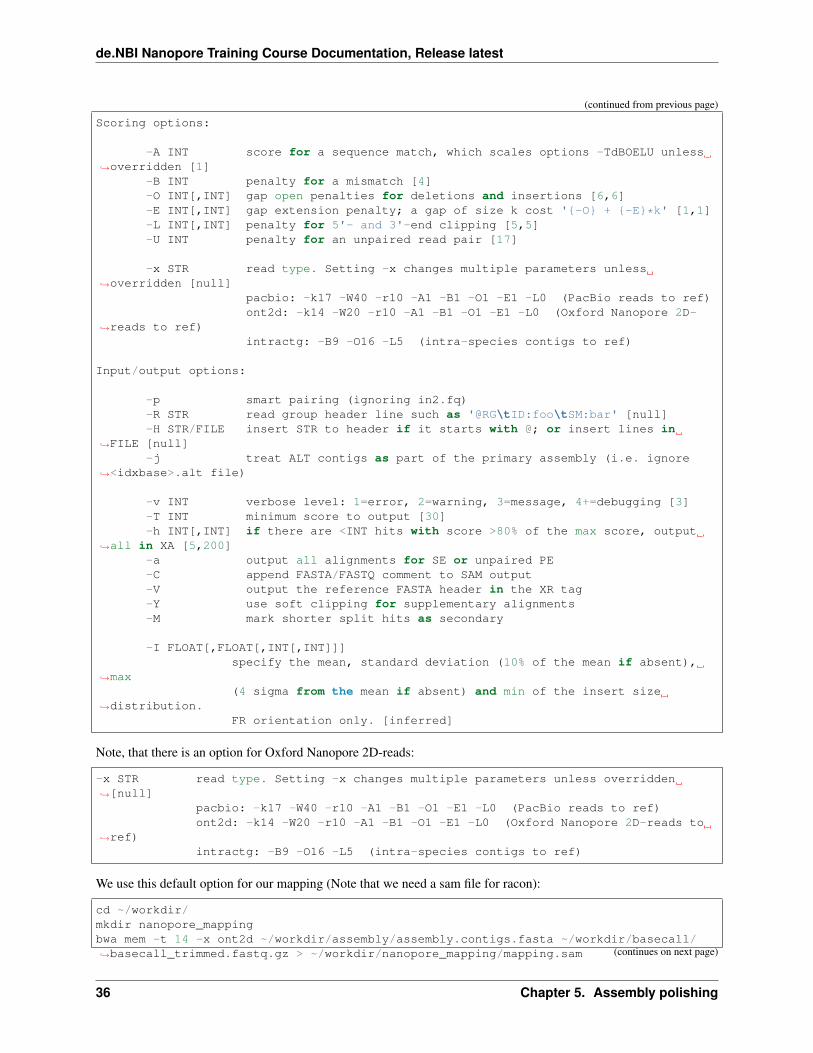
Note, that there is an option for Oxford Nanopore 2D-reads:
-x STR read type. Setting -x changes multiple parameters unless overridden→˓[null]
pacbio: -k17 -W40 -r10 -A1 -B1 -O1 -E1 -L0 (PacBio reads to ref)ont2d: -k14 -W20 -r10 -A1 -B1 -O1 -E1 -L0 (Oxford Nanopore 2D-reads to
→˓ref)intractg: -B9 -O16 -L5 (intra-species contigs to ref)
We use this default option for our mapping (Note that we need a sam file for racon):
cd ~/workdir/mkdir nanopore_mappingbwa mem -t 14 -x ont2d ~/workdir/assembly/assembly.contigs.fasta ~/workdir/basecall/→˓basecall_trimmed.fastq.gz > ~/workdir/nanopore_mapping/mapping.sam (continues on next page)
36 Chapter 5. Assembly polishing

de.NBI Nanopore Training Course Documentation, Release latest
(continued from previous page)
Run racon
Check the usage of racon:
racon --helpusage: racon [options ...] <sequences> <overlaps> <target sequences>
<sequences>input file in FASTA/FASTQ format (can be compressed with gzip)containing sequences used for correction
<overlaps>input file in MHAP/PAF/SAM format (can be compressed with gzip)containing overlaps between sequences and target sequences
<target sequences>input file in FASTA/FASTQ format (can be compressed with gzip)containing sequences which will be corrected
options:-u, --include-unpolished
output unpolished target sequences-f, --fragment-correction
perform fragment correction instead of contig polishing(overlaps file should contain dual/self overlaps!)
-w, --window-length <int>default: 500size of window on which POA is performed
-q, --quality-threshold <float>default: 10.0threshold for average base quality of windows used in POA
-e, --error-threshold <float>default: 0.3maximum allowed error rate used for filtering overlaps
-m, --match <int>default: 5score for matching bases
-x, --mismatch <int>default: -4score for mismatching bases
-g, --gap <int>default: -8gap penalty (must be negative)
-t, --threads <int>default: 1number of threads
--versionprints the version number
-h, --helpprints the usage
Then we can call racon with our mapping, the read file and the assembly file. We use 14 threads to do this:
cd ~/workdir/mkdir raconracon -m 8 -x -6 -g -8 -w 500 -t 14 ~/workdir/basecall/basecall_trimmed.fastq.gz ~/→˓workdir/nanopore_mapping/mapping.sam ~/workdir/assembly/assembly.contigs.fasta >→˓racon/racon.fasta
(continues on next page)
5.2. Assembly polishing with racon and medaka 37

de.NBI Nanopore Training Course Documentation, Release latest
(continued from previous page)
The options:
-m 8 -x -6 -g -8 -w 500
are used, because they were also used for the training of medaka and we want to have similar error profiles of the draft.
References
BWA http://bio-bwa.sourceforge.net/
racon https://github.com/isovic/racon
5.2.2 Polishing with medaka
Medaka is a tool to create a consensus sequence of nanopore sequencing data. This task is performed using neuralnetworks applied a pileup of individual sequencing reads against a draft assembly. It outperforms graph-based methodsoperating on basecalled data, and can be competitive with state-of-the-art signal-based methods whilst being muchfaster.
In earlier courses, we used nanopolish for polishing but it is outperformed by medaka in both runtime and accuracy.
As input medaka accepts reads in either a .fasta or a .fastq file. It requires a draft assembly as a .fasta.
Check the usage of medaka_consensus:
medaka_consensus [-h] -i <fastx>
-h show this help text.-i fastx input basecalls (required).-d fasta input assembly (required).-o output folder (default: medaka).-m medaka model, (default: r941_min_high).
Available: r941_trans, r941_flip213, r941_flip235, r941_min_fast, r941_min_high,→˓ r941_prom_fast, r941_prom_high.
Alternatively a .hdf file from 'medaka train'.-t number of threads with which to create features (default: 1).-b batchsize, controls memory use (default: 200).
-i must be specified.
For comparison, we run medaka on our inital assembly and on the one polished with racon. We use the modelr941_min_high. So we can call medaka with:
medaka_consensus -i basecall/basecall_trimmed.fastq.gz -d assembly/assembly.contigs.→˓fasta -o medaka -t 14 -m r941_min_high
To run medaka on the racon polished assembly:
medaka_consensus -i basecall/basecall_trimmed.fastq.gz -d racon/racon.fasta -o racon_→˓medaka -t 14 -m r941_min_high
Next, we are going to have a short look on assembly results and further polish with pilon.
38 Chapter 5. Assembly polishing

de.NBI Nanopore Training Course Documentation, Release latest
References
medaka https://github.com/nanoporetech/medaka
5.2.3 Assembly evaluation with quast
As usual, we are going to use quast for assembly evaluation:
cd ~/workdirquast.py -t 14 -o ~/workdir/quast_medaka -R ~/workdir/data/Reference.fna ~/workdir/→˓assembly/assembly.contigs.fasta ~/workdir/racon/racon.fasta ~/workdir/medaka/→˓consensus.fasta ~/workdir/racon_medaka/consensus.fasta
QUAST generates HTML reports including a number of interactive graphics. To access these reports, open a filebrowser.
References
quast http://sourceforge.net/projects/quast
5.2.4 Further polishing with pilon
We will further polish with pilon.
As usual, we need to map the data to the assembly and run several pilon rounds:
bwa index ~/workdir/racon_medaka/consensus.fastacd ~/workdirmkdir illumina_mapping_consensusbwa mem -t 14 ~/workdir/racon_medaka/consensus.fasta ~/workdir/data/illumina/Illumina_→˓R1.fastq.gz ~/workdir/data/illumina/Illumina_R2.fastq.gz | samtools view - -Sb |→˓samtools sort - -@14 -o ~/workdir/illumina_mapping_consensus/mapping.sorted.bamsamtools index ~/workdir/illumina_mapping_consensus/mapping.sorted.bamcd ~/workdirmkdir racon_medaka_pilonjava -Xmx32G -jar ~/pilon-1.22.jar --genome racon_medaka/consensus.fasta --fix all --→˓changes --frags illumina_mapping_consensus/mapping.sorted.bam --threads 14 --output→˓racon_medaka_pilon/pilon_round1 | tee racon_medaka_pilon/round1.pilon
Round 2:
bwa index ~/workdir/racon_medaka_pilon/pilon_round1.fastabwa mem -t 14 ~/workdir/racon_medaka_pilon/pilon_round1.fasta ~/workdir/data/illumina/→˓Illumina_R1.fastq.gz ~/workdir/data/illumina/Illumina_R2.fastq.gz | samtools view -→˓-Sb | samtools sort - -@14 -o ~/workdir/illumina_mapping_consensus/mapping_pilon1.→˓sorted.bamsamtools index ~/workdir/illumina_mapping_consensus/mapping_pilon1.sorted.bamjava -Xmx32G -jar ~/pilon-1.22.jar --genome ~/workdir/racon_medaka_pilon/pilon_round1.→˓fasta --fix all --changes --frags illumina_mapping_consensus/mapping_pilon1.sorted.→˓bam --threads 14 --output racon_medaka_pilon/pilon_round2 | tee racon_medaka_pilon/→˓round2.pilon
Round 3:
(continues on next page)
5.2. Assembly polishing with racon and medaka 39

de.NBI Nanopore Training Course Documentation, Release latest
(continued from previous page)
bwa index ~/workdir/racon_medaka_pilon/pilon_round2.fastabwa mem -t 14 ~/workdir/racon_medaka_pilon/pilon_round2.fasta ~/workdir/data/illumina/→˓Illumina_R1.fastq.gz ~/workdir/data/illumina/Illumina_R2.fastq.gz | samtools view -→˓-Sb | samtools sort - -@14 -o ~/workdir/illumina_mapping_consensus/mapping_pilon2.→˓sorted.bamsamtools index ~/workdir/illumina_mapping_consensus/mapping_pilon2.sorted.bamjava -Xmx32G -jar ~/pilon-1.22.jar --genome ~/workdir/racon_medaka_pilon/pilon_round2.→˓fasta --fix all --changes --frags illumina_mapping_consensus/mapping_pilon2.sorted.→˓bam --threads 14 --output racon_medaka_pilon/pilon_round3 | tee racon_medaka_pilon/→˓round3.pilon
Round 4:
bwa index ~/workdir/racon_medaka_pilon/pilon_round3.fastabwa mem -t 14 ~/workdir/racon_medaka_pilon/pilon_round3.fasta ~/workdir/data/illumina/→˓Illumina_R1.fastq.gz ~/workdir/data/illumina/Illumina_R2.fastq.gz | samtools view -→˓-Sb | samtools sort - -@14 -o ~/workdir/illumina_mapping_consensus/mapping_pilon3.→˓sorted.bamsamtools index ~/workdir/illumina_mapping_consensus/mapping_pilon3.sorted.bamjava -Xmx32G -jar ~/pilon-1.22.jar --genome ~/workdir/racon_medaka_pilon/pilon_round3.→˓fasta --fix all --changes --frags illumina_mapping_consensus/mapping_pilon3.sorted.→˓bam --threads 14 --output racon_medaka_pilon/pilon_round4 | tee racon_medaka_pilon/→˓round4.pilon
We have also precomputed the polishing for you, if we are short on time:
cp -r ~/workdir/results/racon_medaka_pilon/ ~/workdir/
References
pilon https://github.com/broadinstitute/pilon/wiki
5.2.5 Assembly evaluation with quast
As usual, we are going to use quast for a final assembly evaluation:
cd ~/workdirquast.py -t 14 -o ~/workdir/quast_final -R ~/workdir/data/Reference.fna ~/workdir/→˓assembly/assembly.contigs.fasta ~/workdir/results/illumina_assembly/contigs.fasta ~/→˓workdir/pilon/pilon_round4.fasta ~/workdir/racon/racon.fasta ~/workdir/racon_medaka/→˓consensus.fasta ~/workdir/racon_medaka_pilon/pilon_round1.fasta ~/workdir/racon_→˓medaka_pilon/pilon_round2.fasta ~/workdir/racon_medaka_pilon/pilon_round3.fasta ~/→˓workdir/racon_medaka_pilon/pilon_round4.fasta ~/workdir/results/nanopolish/polished_→˓genome.fasta
QUAST generates HTML reports including a number of interactive graphics. To access these reports, open a filebrowser.
References
quast http://sourceforge.net/projects/quast
40 Chapter 5. Assembly polishing
de.NBI Nanopore Training Course Documentation, Release latest
5.3 Assembly polishing with nanopolish
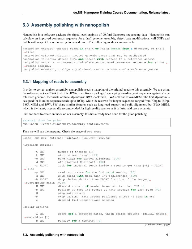
Nanopolish is a software package for signal-level analysis of Oxford Nanopore sequencing data. Nanopolish cancalculate an improved consensus sequence for a draft genome assembly, detect base modifications, call SNPs andindels with respect to a reference genome and more. The following modules are available:
nanopolish extract: extract reads in FASTA or FASTQ format from a directory of FAST5→˓filesnanopolish call-methylation: predict genomic bases that may be methylatednanopolish variants: detect SNPs and indels with respect to a reference genomenanopolish variants --consensus: calculate an improved consensus sequence for a draft→˓genome assemblynanopolish eventalign: align signal-level events to k-mers of a reference genome
5.3.1 Mapping of reads to assembly
In order to correct a given assembly, nanopolish needs a mapping of the original reads to this assembly. We are usingthe software package BWA to do this. BWA is a software package for mapping low-divergent sequences against a largereference genome. It consists of three algorithms: BWA-backtrack, BWA-SW and BWA-MEM. The first algorithm isdesigned for Illumina sequence reads up to 100bp, while the rest two for longer sequences ranged from 70bp to 1Mbp.BWA-MEM and BWA-SW share similar features such as long-read support and split alignment, but BWA-MEM,which is the latest, is generally recommended for high-quality queries as it is faster and more accurate.
First we need to create an index on our assembly, this has already been done for the pilon polishing:
#already done for pilonbwa index ~/workdir/assembly/assembly.contigs.fasta
Then we will run the mapping. Check the usage of bwa mem:
Usage: bwa mem [options] <idxbase> <in1.fq> [in2.fq]
Algorithm options:
-t INT number of threads [1]-k INT minimum seed length [19]-w INT band width for banded alignment [100]-d INT off-diagonal X-dropoff [100]-r FLOAT look for internal seeds inside a seed longer than {-k} * FLOAT
→˓[1.5]-y INT seed occurrence for the 3rd round seeding [20]-c INT skip seeds with more than INT occurrences [500]-D FLOAT drop chains shorter than FLOAT fraction of the longest
→˓overlapping chain [0.50]-W INT discard a chain if seeded bases shorter than INT [0]-m INT perform at most INT rounds of mate rescues for each read [50]-S skip mate rescue-P skip pairing; mate rescue performed unless -S also in use-e discard full-length exact matches
Scoring options:
-A INT score for a sequence match, which scales options -TdBOELU unless→˓overridden [1]
-B INT penalty for a mismatch [4]
(continues on next page)
5.3. Assembly polishing with nanopolish 41

de.NBI Nanopore Training Course Documentation, Release latest
(continued from previous page)
-O INT[,INT] gap open penalties for deletions and insertions [6,6]-E INT[,INT] gap extension penalty; a gap of size k cost '{-O} + {-E}*k' [1,1]-L INT[,INT] penalty for 5'- and 3'-end clipping [5,5]-U INT penalty for an unpaired read pair [17]
-x STR read type. Setting -x changes multiple parameters unless→˓overridden [null]
pacbio: -k17 -W40 -r10 -A1 -B1 -O1 -E1 -L0 (PacBio reads to ref)ont2d: -k14 -W20 -r10 -A1 -B1 -O1 -E1 -L0 (Oxford Nanopore 2D-
→˓reads to ref)intractg: -B9 -O16 -L5 (intra-species contigs to ref)
Input/output options:
-p smart pairing (ignoring in2.fq)-R STR read group header line such as '@RG\tID:foo\tSM:bar' [null]-H STR/FILE insert STR to header if it starts with @; or insert lines in
→˓FILE [null]-j treat ALT contigs as part of the primary assembly (i.e. ignore
→˓<idxbase>.alt file)
-v INT verbose level: 1=error, 2=warning, 3=message, 4+=debugging [3]-T INT minimum score to output [30]-h INT[,INT] if there are <INT hits with score >80% of the max score, output
→˓all in XA [5,200]-a output all alignments for SE or unpaired PE-C append FASTA/FASTQ comment to SAM output-V output the reference FASTA header in the XR tag-Y use soft clipping for supplementary alignments-M mark shorter split hits as secondary
-I FLOAT[,FLOAT[,INT[,INT]]]specify the mean, standard deviation (10% of the mean if absent),
→˓max(4 sigma from the mean if absent) and min of the insert size
→˓distribution.FR orientation only. [inferred]
Note, that there is an option for Oxford Nanopore 2D-reads:
-x STR read type. Setting -x changes multiple parameters unless overridden→˓[null]
pacbio: -k17 -W40 -r10 -A1 -B1 -O1 -E1 -L0 (PacBio reads to ref)ont2d: -k14 -W20 -r10 -A1 -B1 -O1 -E1 -L0 (Oxford Nanopore 2D-reads to
→˓ref)intractg: -B9 -O16 -L5 (intra-species contigs to ref)
We use this default option for our mapping:
cd ~/workdir/mkdir nanopore_mappingbwa mem -t 14 -x ont2d ~/workdir/assembly/assembly.contigs.fasta ~/workdir/basecall/→˓ONT.fastq.gz | samtools view - -Sb | samtools sort - -@14 > ~/workdir/nanopore_→˓mapping/mapping.sorted.bam
We need to convert the resulting sam file to a sorted and indexed bam file:
42 Chapter 5. Assembly polishing

de.NBI Nanopore Training Course Documentation, Release latest
samtools index ~/workdir/nanopore_mapping/mapping.sorted.bam
References
BWA http://bio-bwa.sourceforge.net/
samtools http://www.htslib.org/
5.3.2 Indexing fastq from 1D Basecalling
In order to prepare our 1D fastq file for nanopolish (so that the tool can find the original raw files), we need to indexthe fastq files from the 1D basecalling again with nanopolish:
nanopolish index -d ~/workdir/data/fast5/ ~/workdir/basecall/ONT.fastq.gz
5.3.3 Call nanopolish
Now that all pieces are together, we can call nanopolish with:
• our assembly
• our indexed fastq files from 1D basecalling
• our mapping of 1D fastq vs. our assembly
Create a directory first:
cd ~/workdirmkdir nanopolish
Call nanopolish:
python /usr/local/lib/nanopolish/scripts/nanopolish_makerange.py ~/workdir/assembly/→˓assembly.contigs.fasta | parallel --results nanopolish.results -P 7 nanopolish→˓variants --consensus -o ~/workdir/nanopolish/polished.{1}.vcf -w {1} -r ~/workdir/→˓basecall/ONT.fastq.gz -b ~/workdir/nanopore_mapping/mapping.sorted.bam -g ~/workdir/→˓assembly/assembly.contigs.fasta -t 2
This will run a few hours over night and we can get to dinner. :)
Next morning, we need to create the corrected fasta file from the generated vcf:
nanopolish vcf2fasta -g ~/workdir/assembly/assembly.contigs.fasta ~/workdir/→˓nanopolish/polished.*.vcf > ~/workdir/nanopolish/polished_genome.fasta
5.3.4 Assembly evaluation with quast
We are going to evaluate our polished assembly. To call quast.py we have to provide a reference genome and anassembly as before. We will include our original canu assembly for comparison:
quast.py -t 14 -o ~/workdir/quast_nanopolished_assembly -R ~/workdir/Data/Reference/→˓CXERO_10272017.fna ~/workdir/polishedContig.fasta ~/workdir/canu_assembly/→˓largestContig.fasta
5.3. Assembly polishing with nanopolish 43
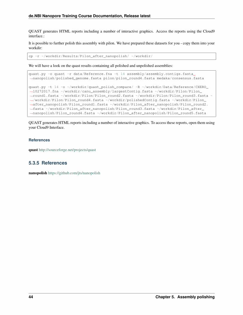
de.NBI Nanopore Training Course Documentation, Release latest
QUAST generates HTML reports including a number of interactive graphics. Access the reports using the Cloud9interface.:
It is possible to further polish this assembly with pilon. We have prepared these datasets for you - copy them into yourworkdir:
cp -r ~/workdir/Results/Pilon_after_nanopolish/ ~/workdir/
We will have a look on the quast results containing all polished and unpolished assemblies:
quast.py -o quast -r data/Reference.fna -t 14 assembly/assembly.contigs.fasta→˓nanopolish/polished_genome.fasta pilon/pilon_round4.fasta medaka/consensus.fasta
quast.py -t 14 -o ~/workdir/quast_polish_compare/ -R ~/workdir/Data/Reference/CXERO_→˓10272017.fna ~/workdir/canu_assembly/largestContig.fasta ~/workdir/Pilon/Pilon_→˓round1.fasta ~/workdir/Pilon/Pilon_round2.fasta ~/workdir/Pilon/Pilon_round3.fasta ~→˓/workdir/Pilon/Pilon_round4.fasta ~/workdir/polishedContig.fasta ~/workdir/Pilon_→˓after_nanopolish/Pilon_round1.fasta ~/workdir/Pilon_after_nanopolish/Pilon_round2.→˓fasta ~/workdir/Pilon_after_nanopolish/Pilon_round3.fasta ~/workdir/Pilon_after_→˓nanopolish/Pilon_round4.fasta ~/workdir/Pilon_after_nanopolish/Pilon_round5.fasta
QUAST generates HTML reports including a number of interactive graphics. To access these reports, open them usingyour Cloud9 Interface.
References
quast http://sourceforge.net/projects/quast
5.3.5 References
nanopolish https://github.com/jts/nanopolish
44 Chapter 5. Assembly polishing

CHAPTER 6
Genome annotation
We will annotate our (almost) finished genome sequence.
6.1 Annotating the genome with prokka
The multiplex capability and high yield of current day DNA-sequencing instruments has made bacterial whole genomesequencing a routine affair. The subsequent de novo assembly of reads into contigs has been well addressed. The finalstep of annotating all relevant genomic features on those contigs can be achieved slowly using existing web- and email-based systems, but these are not applicable for sensitive data or integrating into computational pipelines. Prokka is acommand line software tool to fully annotate a draft bacterial genome in about 10 min on a typical desktop computer.It produces standards-compliant output files for further analysis or viewing in genome browsers.
In order to call prokka, we first need to shorten the name of our largest contig (the genome sequence) because it hasgotten quite long due to several pilon rounds. We use a simple shell command to do that:
mkdir Annotationcat ~/workdir/racon_medaka_pilon/pilon_round4.fasta | sed -e 's/>tig.*/>genome_→˓sequence/g' > ~/workdir/Annotation/genome.fasta
Then we call Prokka with the genome sequence and specify an output directory:
prokka ~/workdir/Annotation/genome.fasta --outdir ~/workdir/Annotation/prokka/
We will use a genome browser to look at the annotated genome. For this, you have to
1. open a terminal window on your local workstation
2. download the prokka files using Cloud9
3. start ‘IGV: Integrative Genomics Viewer‘_
Here is the command to open the IGV on your local workstation:
/vol/cmg/bin/igv.sh
45

de.NBI Nanopore Training Course Documentation, Release latest
Now let’s look at the annoated genome in IGV. Use the menu Genomes->Load Genome from File...
6.1.1 References
prokka http://www.vicbioinformatics.com/software.prokka.shtml
IGV http://www.broadinstitute.org/igv/
46 Chapter 6. Genome annotation


