Electronic copy available at: http://ssrn.com/abstract=1012093 Density and the Journey to Work by David M. Levinson and Ajay Kumar corresponding author: David M. Levinson submitted to: Growth and Change original date: December 31, 1995 revision date:June 29, 1996 final revision date: November 5, 1996 ABSTRACT This paper evaluates the influence of residential density on commuting behavior across U.S. cities while controlling for available opportunities, the technology of transportation infrastructure, and individual socio- economic and demographic characteristics. The measures of metropolitan and local density are addressed separately. We suggest that metropolitan residential density serves principally as a surrogate for city size. We argue that markets react to high interaction costs found in large cities by raising density rather than density being a cause of those high costs. Local residential density measures relative location (accessibility) within the metropolitan region as well as indexing the level of congestion. We conduct regressions to predict commuting time, speed, and distance by mode of travel on a cross-section of individuals nationally and city by city. The results indicate that residential density in the area around the tripmaker’s home is an important factor: the higher the density the lower the speed and the shorter the distance. However, density’s effect on travel time is ambiguous, speed and distance are off-setting effects on time. The paper suggests a threshold density at which the decrease in distance is overtaken by the congestion effects, resulting in a residential density between 7,500 and 10,000 persons per square mile (neither the highest nor lowest) with the shortest duration auto commutes. Published as: Levinson, David and Ajay Kumar (1997). Density and the Journey to Work. Growth and Change 28:2 147-172
Transcript
Electronic copy available at: http://ssrn.com/abstract=1012093
Density and the Journey to Work
by David M. Levinson
and Ajay Kumar
corresponding author:
David M. Levinson
submitted to: Growth and Change
original date: December 31, 1995
revision date:June 29, 1996
final revision date: November 5, 1996
ABSTRACTThis paper evaluates the influence of residential density on commutingbehavior across U.S. cities while controlling for available opportunities,the technology of transportation infrastructure, and individual socio-economic and demographic characteristics. The measures ofmetropolitan and local density are addressed separately. We suggest thatmetropolitan residential density serves principally as a surrogate for citysize. We argue that markets react to high interaction costs found in largecities by raising density rather than density being a cause of those highcosts. Local residential density measures relative location (accessibility)within the metropolitan region as well as indexing the level of congestion.We conduct regressions to predict commuting time, speed, and distance bymode of travel on a cross-section of individuals nationally and city by city.The results indicate that residential density in the area around thetripmaker’s home is an important factor: the higher the density the lowerthe speed and the shorter the distance. However, density’s effect on traveltime is ambiguous, speed and distance are off-setting effects on time. Thepaper suggests a threshold density at which the decrease in distance isovertaken by the congestion effects, resulting in a residential densitybetween 7,500 and 10,000 persons per square mile (neither the highestnor lowest) with the shortest duration auto commutes.
Published as: Levinson, David and Ajay Kumar (1997). Density and the Journey to Work. Growth and Change 28:2 147-172
Electronic copy available at: http://ssrn.com/abstract=1012093
INTRODUCTION
The inter-relationships among density, city size, demographics, and travel demand
patterns have long been discussed at the national or metropolitan scale (Voorhees 1968;
Richardson 1973, Steiner 1994, Frank and Pivo 1994). With recent concerns about
damage to air quality caused by highway transportation, this issue has become more
relevant for public policy (Bae 1992). Debate remains about many of the details of the
interactions between variables and their potential implication for transportation policy.
Newman and Kenworthy (1992), for instance, criticize earlier investigations into
the issue of the effects of urban form on travel, stating that “U.S. data constitute a poor
sample for examining the effects of density on travel and gasoline use, as there is very
little density variation on a metropolitan basis.” They conclude that the higher the
density, the lower the gasoline consumption, suggesting an exponential relationship
between density and gasoline use, and find significant effects above 30 persons per
hectare (ha) or 7800 persons per square mile. This is consistent with Pushkarev and
Zupan (1977), who analyzed data on the New York region and found that there exists a
significant positive relationship between density and transit trips. They also found that,
on average, lower income households travel less than other households at all densities.
Goodwin (1975) used the 1971-72 British national travel survey to evaluate the
relationship between density and several travel related characteristics, concluding that
households in high density areas made the same number of trips overall, but fewer by
automobile.
However, analyzing data from both the Federal Highway Administration’s
“Highway Statistics 1990” and the Texas Transportation Institute, Dunphy and Fisher
(1994) argue that metropolitan residential density explains only 15% of the variation in
per capita VMT among metropolitan areas over one million persons. Gordon et al.
(1989a), using data derived from Landsat photographs to compute the ratio of residential
population to residential land at the metropolitan level, conclude that metropolitan
residential densities and commuting times are positively associated.
The conflicting findings between researchers indicate a difficulty in determining
whether density increases or reduces total commuting time and distance. In part that is
due to multiple measurements of density: local vs. metropolitan and residential vs.
employment; in part it is the ambiguity about what a “density” measurement is really
measuring: is local density really capturing the number of people per unit area, the level
of congestion, or the distance from the center(s) of the region (and implicitly the distance
to other people), is metropolitan density really just capturing city size? The answer to
Published as: Levinson, David and Ajay Kumar (1997). Density and the Journey to Work. Growth and Change 28:2 147-172
these questions has important implications for land use policies which hope to change
travel behavior by changing land use densities.
We argue that at the metropolitan level, average density is principally a surrogate
for city size. Aside from its accessibility benefits (agglomeration economies), increased
density brings about costs that are undesirable (less space per person, more expensive
construction, higher land costs, congestion). Thus densification, like polycentricity, is
primarily a market response to contain or reduce otherwise high interaction costs (in
particular journey to work times, but also including other travel costs such as those of
firm to firm interactions (Sivitanidou 1995) and non-work travel (Handy 1993)) found as
cities increase in population, rather than a cause of those travel times.
Within the city, density remains largely a measure of distance from the center(s)
of the region. Researchers agree that local density is positively associated with non-auto
mode shares for several reasons, higher congestion in the urban core, greater frequency of
transit service, and lowered access to transit times. Density’s effect on overall
commuting times is less straight-forward. Clearly the higher the density (and the closer
to the center of the region) the more possible destinations that can be reached in the same
distance. Just as clearly density and congestion are paired, leading to slower speeds, at
least by the automobile. Because congestion effects are non-linear, at low flows travel
times are almost unaffected by the marginal traveler but above a critical threshold each
one percent increase in traffic increases time by more than one percent, we expect a non-
linear association between density and highway travel times. When increasing density
from a lower level, the gain in coverage by auto outweighs the reduction in speed, at
higher densities the opposite holds. We also note that the highest density neighborhoods
are only found in the centers of the largest metropolitan areas.
We use the 1990/91 Nationwide Personal Transportation Survey (NPTS) to
analyze the effect of local and metropolitan residential density, the number of edge
cities, rate of growth, highway speed, transit availability, and demographics and socio-
economics on the commuting time, distance, and speed of individual commuters. In the
following section the relationships between urban structure and travel behavior are
discussed in order to develop specific hypotheses to test with the available database. That
section examines the influence of a variety of variables (residential density, city size,
growth rate, transportation network structure, income, gender, and age) on time, speed
and distance and presents general observations and hypotheses. Then the NPTS database
used in this analysis is discussed. These discussions are followed by the results from
several regression analyses across cities nationally, individuals nationally, and
Published as: Levinson, David and Ajay Kumar (1997). Density and the Journey to Work. Growth and Change 28:2 147-172
individuals in specific cities to isolate inter- and intra-metropolitan variation. The paper
concludes that while density matters statistically, particularly regarding distance and
speed, its influence is relatively weak - suggesting that density makes a poor choice as a
policy instrument to influence individual travel times.
THEORY AND HYPOTHESES
As noted in the introduction, the relationship between density and travel behavior
is complex, the empirical pieces are not entirely in concord. Furthermore, theories of
urban economics do not give unambiguous predictions about the amount of travel
undertaken (in terms of time or distance) as a function of key spatial variables, primarily
because the axioms of the standard model require resolving empirical factors.
First, it has been long observed that the level of interaction between any two
places declines with separation (Isard 1956), that is, the desirability of a commute
between home and work declines with increasing travel time, cost, and effort. The
gravity model, which measures this phenomenon, has been confirmed many times
(Mitchelson and Wheeler 1986, Scott 1988, Cervero 1989, Levinson and Kumar 1995a).
The time spent traveling, to work and other destinations, must be nested within a broader
activity framework (Pas 1980, Levinson and Kumar 1995b), and time spent traveling
necessarily reduces the available time for other activities, which helps explain the size of
this disutility.
Second, geometry dictates that the cumulative number of opportunities (for
instance jobs or houses) increases with the area covered. In the case of uniform density,
the number increases from a point as the square of distance, though it must be recognized
that opportunities are not evenly distributed. For instance, resident workers of larger
cities have more jobs available at farther distances than do residents of smaller cities,
who more quickly reach the boundary of the metropolitan region and levels of very low
intensity use. It has generally been observed, and confirmed in Table 1, that larger cities
have longer average commutes (in both distance and time).
It is apparent that the first and second factors are offsetting, while costs rise with
distance, so do opportunities. Because commuters are neither time minimizing nor
opportunity maximizing, some trade-off between the two takes place, leaving commutes
longer than the minimum required (Giuliano and Small 1993), but still constraining the
size of the city.
Published as: Levinson, David and Ajay Kumar (1997). Density and the Journey to Work. Growth and Change 28:2 147-172
To unpack this process, commuting distance, speed, and duration can be estimated
as a function of several measurable factors. Conceptually, we can view the expected
commuting time (distance, speed) for an individual to depend on several factors:
residential density which represents both the spatial location of home as well as
congestion levels, variables representing the number and pattern of employment
opportunities available and how fast the number is changing, transportation technology
and level of service, and individual socioeconomic and demographic factors. This
section presents specific hypotheses of the influence of local and metropolitan density,
the number of edge cities, the metropolitan growth rate, the use of freeways and presence
of heavy rail, and demographics and socio-economics (income, gender, and age) on travel
time, speed, and distance separately for auto and transit users. The tests of the
hypotheses using ordinary least squares regression are presented in subsequent sections.
Metropolitan Density
Consistent with theory, average metropolitan residential density, and thus the
proportion of individuals living at specific (local) residential densities within a city, is
highly dependent on city size. While it would be desirable to distinguish spatial extent
and density, the variables are too highly correlated in the available data to be able to do
so with accuracy. Markets react to the increased distance that would otherwise need to be
covered as cities expand horizontally over space in several ways. Historically, density
was increased, both uniformly and particularly in downtown. More recently, multiple
centers were spawned. This suggests that density (or polycentricity), rather than being a
cause of high travel times, may be more properly viewed as a response to otherwise long
distances designed to contain commuting costs. Therefore, research which finds a
positive association of average commuting duration with density (or the number of
centers), may have found what historically explains the density (or polycentricity), rather
than vice versa.
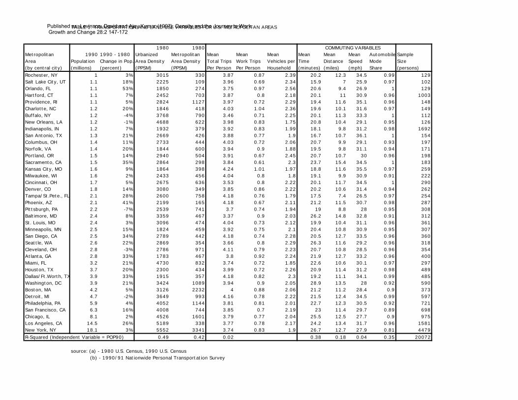
Table 1 shows the land use variables (1990 population, ten year growth rate, and
metropolitan and urbanized area density) as well as transportation variables (mean travel
time, distance, speed, trip frequency, and vehicle ownership) for each Metropolitan
Statistical Area (MSA) or Consolidated Metropolitan Statistical Area (CMSA), as
defined by the U.S. Bureau of the Census, with a population greater than 1,000,000
persons. The cities range in size from the Rochester, NY MSA (one million persons), to
the New York City CMSA (over 18 million persons). Sample rates vary between cities as
several Metropolitan Planning Organizations (MPO) (in particular New York and
Indianapolis) paid for the collection of additional responses.
Published as: Levinson, David and Ajay Kumar (1997). Density and the Journey to Work. Growth and Change 28:2 147-172
As shown in Table 1, urbanized area residential density (URBDENS) and city
size are positively correlated, and clearly larger cities have longer travel times.
Furthermore, this was found in work by Gordon et al. (1989b), arguing that low density
metropolitan areas with their decentralized employment centers facilitate shorter work
trips and high density areas are subject to congestion. The relationships between
residential density and travel parameters (travel time, distance, speed) are re-examined
here by looking at a cross-section of cities in the United States. We argue that if
metropolitan density is positively associated with high commuting times, it is the density
which is a consequence of trying to reduce otherwise higher interaction costs (in times
past) in a city, which without increasing density would spread over a larger space, and
not the other way around. Density, after controlling for city size, would be associated
with shorter distances and slower speeds, but since density and city size are highly
correlated we cannot use both variables in the regressions and get meaningful results, a
priori the results will be uncertain.
Local Residential Density
Local residential density is the best available measure in the 1990 NPTS dataset
of relative location of the household within the metropolitan region. As noted above,
there are theoretical reasons that density and non-auto mode shares should be associated,
and possibly density and trip rates due to opportunities for trip chaining. However there is
no theoretical reason that density per se should have any effect on journey to work travel
time. We are thus taking the position that, as a determinant of travel time, the variable
representing local residential density measures most importantly congestion and distance
from the center(s), rather than density itself.
First, the travel time between places depends on the speed of the transportation
network, a function of traffic flow, which is strongly correlated with density. At
uncongested levels of traffic, a one percent increase in traffic flow on a section of
roadway increases travel time by far less than one percent; at congested levels, a one
percent increase in flow increases time by far more than one percent.
Second, intensity of use tends to decline with distance from the city’s center(s),
resulting in shorter distance trips in high density areas . However the relationship
between density and distance from the center is not fixed. Over the past century, due to
congestion costs coupled with the increasing accessibility in lower density areas
associated with the new technologies of the automobile and freeway, the CBD-density
gradient has been shown to be declining in U.S. cities (Mills 1972, Heikkila et al. 1989).
Published as: Levinson, David and Ajay Kumar (1997). Density and the Journey to Work. Growth and Change 28:2 147-172
The emergence of polycentric cities further reflects the declining relative importance of
the single center in a city, and suggests an increasing disparity between density and
distance from the dominant regional center (the central business district), though not
necessarily from secondary suburban centers (Giuliano and Small 1991, Gordon et al.
1986, Greene 1980, , McDonald 1987, and McDonald and Prather 1994).
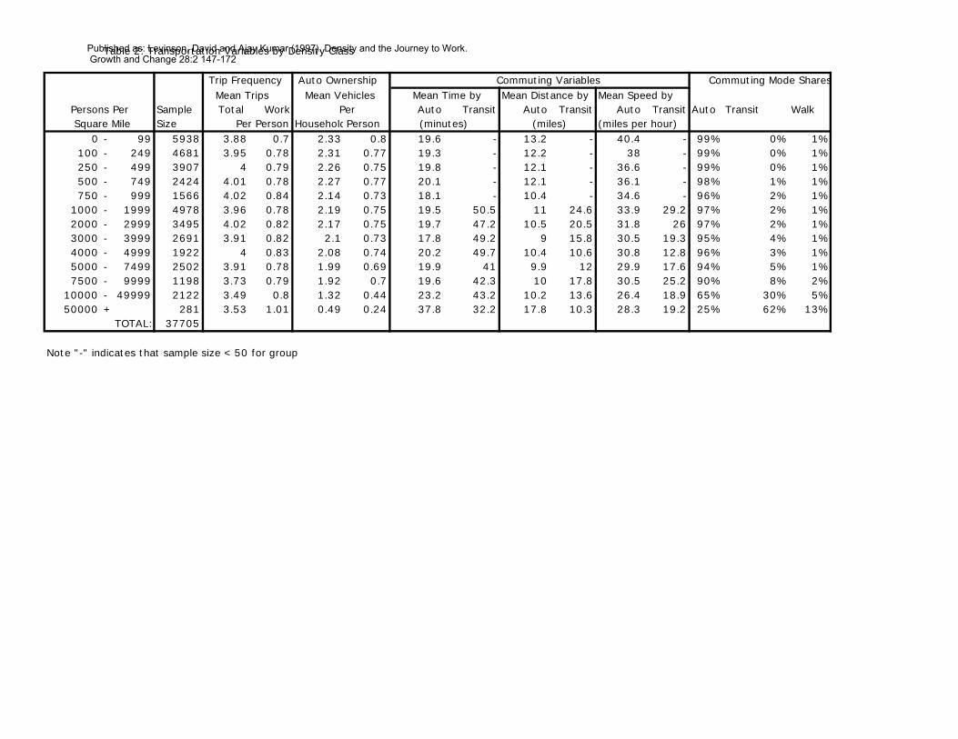
Table 2 shows that by auto, home to work travel times are fairly constant for
densities below 10,000 ppsm; however, travel times increase at densities above 10,000
ppsm. Mean time by auto increases from 20 minutes at densities below 10,000 to 38
minutes in areas above 50,000 ppsm. By transit, home to work travel times remain
approximately 50 minutes below 5000 ppsm; 40 minutes between 5000 and 50,000 ppsm;
and about 32 minutes above 50,000 ppsm. A comparison of auto and transit can be seen
with the ratio of transit time to auto time. At values greater than 1, transit time exceeds
auto time. This variable drops from 2.9 (transit trips taking about three times as long as
auto trips) at densities less than 4000 ppsm to 0.9 at densities greater than 50,000 ppsm,
beyond which transit mode share exceeds auto mode share. Distance and speed both
decline with increased density.
Two standard hypotheses concerning density are tested. The first is that density is
negatively associated with trip speed for all modes of travel. Density and congestion
typically go hand in hand, so this relationship is expected. The second hypothesis is that
density is negatively associated with commuting distance. As noted before, density
declines with distance from the center of the region. Also city centers typically have high
job to housing ratios. Therefore, due to high job accessibility in high density residential
neighborhoods we expect the second hypothesis to be borne out in the data. Both
hypotheses will be confirmed if we find a declining coefficient on the density variables in
the distance and speed regressions.
The third hypothesis should concern travel time. But because density and speed
are both expected to be negatively related to density, the effect on commuting time
depends on the magnitude of the other relationships. After examining the data, we
believe that higher densities will reduce automobile travel time up to a point (between
7500 and 10,000 persons per square mile), and above that level, auto times will rise
because the speed reduction outweighs the density reduction. Because we suppress that
density class, in the automobile regression we expect to find that the sign on the
population density variables will be positive in all cases, and rising as the density class is
farther from the suppressed class. We expect to have a “U” shaped curve of density on
the X axis and travel time on the Y axis, with the base of the “U” being the suppressed
density class.
Published as: Levinson, David and Ajay Kumar (1997). Density and the Journey to Work. Growth and Change 28:2 147-172
Centricity
Land use is not evenly distributed; rather centers, by definition, have more
opportunities per unit area than does the periphery. If cities increased in population
without any change in density, they would extend farther in space and commutes would
become longer. To reduce overall interaction costs (journey to work, non-work, and firm
to firm) it becomes desirable to build at higher densities in certain locations, which then
become the regional center(s).
Theory suggests, that after controlling for city size (or metropolitan density), the
more monocentric city will have higher commuting times for automobile commuters,
since the primary reason for polycentricity is to contain or reduce commuting costs. On
the other hand, since polycentricity (like density discussed above) is a response to already
high commuting times, the statistical association may come in the other direction. It is
important to recognize that cause and effect here run in both directions as individuals and
firms mutually co-locate in response to congestion costs, and thus reshape those costs.
Two key issues are the degree of concentration or clustering both within and outside the
central city and the distribution of employment relative to population.
However, since there is no measure of the location of individual’s workplace in
the NPTS dataset, we are drawn to use surrogates. Gordon et al (1989b) use the
proportion of metropolitan employment located in the MSA’s central city as an
explanatory factor for travel time to work and find them to be positively associated. That
measure indicates the degree of monocentricity, but unfortunately relies on a central city
boundaries which are politically rather than economically defined.
Our measure (EDGECITY) looks at the number of suburban activity centers in
the metropolitan area (Edge Cities in the terminology of Garreau (1991)) as a measure of
polycentricity, loosely capturing the amount of clustering of jobs outside the central city.
We use Garreau’s list, which he obtained using the five part definition of: five million
square feet of leasable office space, six hundred thousand square feet of retail, an
importer of workers to fill to jobs, a perception as a mixed use destination, and a history
that 30 years before it was not such a center. Clearly this is associated with city size,
though non-linearly; only when a city becomes sufficiently large is it worthwhile for
firms to lose some firm to firm agglomeration economies to achieve an advantage in the
labor market.
Published as: Levinson, David and Ajay Kumar (1997). Density and the Journey to Work. Growth and Change 28:2 147-172
Growth Rate
The rate at which opportunities change may also influence travel times.
Individuals typically only relocate a job or home every few years, they cannot respond
instantly to faster growth and changes in opportunities. Because relocation costs are not
zero, a changing city size, indicative of the absence of equilibrium, may impact travel
times. We use a variable (GROWRATE) expressing the percentage population growth
between 1980 and 1990. A growing city may provide greater opportunities for
households and economic establishments to relocate, resulting in shorter time and
distance commutes. Alternatively, a growing city may have difficulty providing adequate
transportation infrastructure in a timely fashion (hence the rise of growth management in
many fast growing suburbs in the United States) resulting in longer commutes. In
numerous studies it has been shown that total travel has been growing faster than
transportation network capacity. Insufficient capacity may lead to higher than average
travel times. Growth may also be a surrogate for the sun belt urban form more than
change within a city, therefore, this variable needs to be treated with caution.
Transportation Technology
Commuting time is a function of the available technology. A higher speed
technology, ceteris paribus, will lead to shorter duration commutes. But since duration
also depends on distance, and the higher speeds can be used to extend commuting range,
the impacts of technology will have to be determined empirically. There is the
compounding factor of modal investment strategies. Some cities have chosen to invest in
heavy rail systems, often at the expense of highways. This should increase the travel time
of highway commuters.
Transportation investments vary between cities; typically, newer cities have more
freeways, older cities have more mass transit. A dummy variable (RAILCITY), takes the
value 1 for those cities with a heavy rail system (Atlanta, Baltimore, Boston, Chicago,
Cleveland, Miami, New York, Philadelphia, San Francisco, Washington DC) and 0
otherwise. Presence of a rail system is an important variable explaining the organization
of city structure. Typically, cities with rail have a denser central area and higher densities
around stations. A city, by choosing to invest its infrastructure dollars in a rail system
may preclude that money from being spent on highways, thereby leading to lower speeds
and possibly higher travel times by auto.1 Further research could treat rail mileage (by
type of facility, e.g. light rail or heavy rail) as a measure of transit availability. The
Published as: Levinson, David and Ajay Kumar (1997). Density and the Journey to Work. Growth and Change 28:2 147-172
hypothesis tested is that presence of heavy rail will be positively associated with distance
and speed for transit users and negatively associated with speed for auto commuters.
As with land use patterns, transportation networks vary both between and within
cities. Because of increased traffic density, speeds on links in areas of higher density
near the “center” tend to be lower than speeds on links at the periphery. The variable
FREECITY ranges from 0 to 1, and represents the total share of automobile travel (both
work and non-work trips) in a city that takes place on freeways or other limited access
roadways. This variable was computed from the NPTS, which asked a subsample in each
city specific questions on the mileage of each trip on one of four classes of roadway. It is
our hypothesis that freeway-orientation will be positively associated with auto speeds,
and thus will have trips of longer distances to take advantage of them.
Income
Income is expressed as the ratio of household income for an individual to median
metropolitan income in their city (INCRATIO). By controlling for metropolitan income
levels it is hoped to alleviate some of the problems associated with comparing income
levels in different cities. Gordon et al. (1989b) argue that high income households have
more choice in residential location, implying that these households can choose good
housing if it is close to the workplace. Similarly, high income households may place a
higher dollar value on time and be more willing to substitute money for commuting time.
Both factors may lead to shorter travel times in the polycentric urban model. However,
in the monocentric city, travel distances have typically been found to be longer for high
income persons, who more often live in the suburbs.
The degree to which income is related to travel time is thus a function of urban
structure and the extent of decentralization. Results obtained using median income of a
city in an aggregate analysis mask different costs of living found in different cities, and
may be different than those obtained using relative household income at the individual
level. Higher income is also related to increased professional specialization, which
should result in longer distance work trips. However, household income also masks the
relationship of personal income on travel behavior in two-worker households. If a greater
proportion of higher income households live in the suburbs, while central city office jobs
are higher paying, longer distance and time commutes are expected to result, giving
higher speeds obtained on the longer suburban portion of the trip.
Published as: Levinson, David and Ajay Kumar (1997). Density and the Journey to Work. Growth and Change 28:2 147-172
Gender and Age
Gender and age are considered in the individual regressions. The variable
reflecting gender (MALE) is expressed as a binary variable taking the value 1 if the
individual is male and 0 if female or not reported. AGExx-yy is a series of dummy
variables representing cohorts from 16-20, 20-30, 30-40, 40-50, 50-60, 60-70 and 70+,
with the cohort representing 30-40 suppressed. (In the city by city regressions, because of
smaller sample sizes, we used two cohorts, defined by a dummy variable ADULT if the
individual was between the ages of 18 and 65.) Peters and MacDonald (1994) review of
the literature shows that men commute longer than women, with various hypotheses put
forward relating to the relative importance of the home and nature of the job. We also
expect working age adults to have longer commutes than those below 20 or above 65, as
full-time jobs are typically farther afield than part-time.
DATA
The 1990/91 Nationwide Personal Transportation Survey (NPTS), used in this
study, consists of 21,000 household interviews and 47,000 persons making almost
150,000 trips. Additional information about the site of the interviewee (such as
residential density) was added after the interview. The survey collected data on
household demographics, income, vehicle availability, all trips made on the survey day,
long trips made over a two week period, and traffic accidents within the past five years.
Trip characteristics included departure time, distance and duration of the trip, trip purpose
and mode, and the vehicle used.
The key land use variables in our study are the population density of the
residential zip code from the NPTS dataset and a number of other variables obtained from
the Census, including metropolitan size, urbanized and metropolitan population density
in 1980 and 1990 (USDOT 1990; Bureau of Census 1984, 199 1). Some discussion of the
measure of local population density measure used here is warranted. Households were
asked to provide their home postal area, or zip code, as a geographic reference. The zip
code was then matched to an external data set containing population and area estimates.
Population per square mile (ppsm) was calculated for each zip code area and collapsed to
the classes shown in the tables presented in this paper. It should be noted that population
density thus computed may vary widely between zip codes because of the inclusion of
undeveloped land in the area estimates. Lower density areas are expected to have more
undeveloped land included in the area measurement of zip code than high density areas.
While it would be desirable to have estimates of developed land density by land use type
Published as: Levinson, David and Ajay Kumar (1997). Density and the Journey to Work. Growth and Change 28:2 147-172
at a local level, this data was unavailable. However, the available information is still
useful for understanding the broader relationship between density and travel patterns.
National travel surveys conducted in 1969, 1977, and 1983 did not record population
density, precluding this type of analysis. In addition, as discussed above, it is noted that
density computed this way likely acts as a surrogate for distance from the center of the
metropolitan region. While the monocentric urban form is becoming polycentric,
density still tends to decline with distance from the center. It was not possible to separate
the effects of density and distance in this database, as only the residential density variable
was provided and there was no similar variable indicating distance from the center of the
region, and so they are treated together.
RESULTS
Four sets of regressions were performed to test the hypotheses in various ways.
These are shown in a number of tables which are addressed one by one in the following
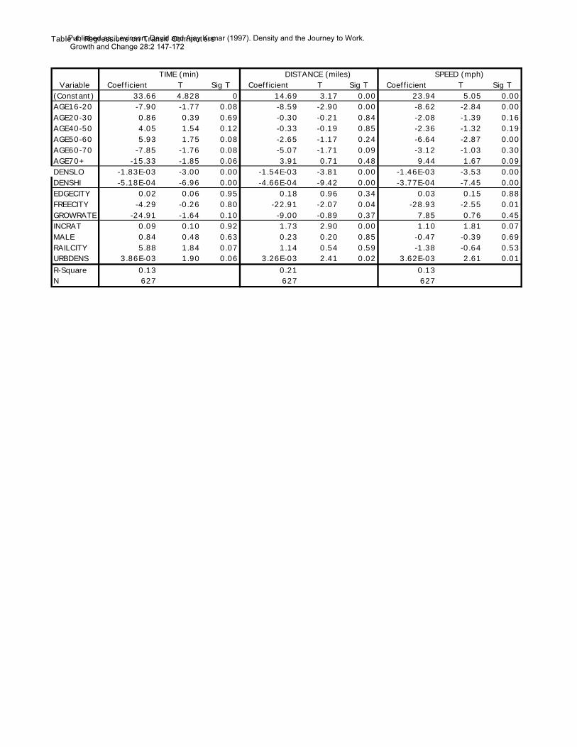
subsections. Table 3 records the regressions on time, speed, and distance of 8651
individual automobile commuters across the country; Table 4 which looks at 627
individual transit commuters; Charts 1,2, and 3, which summarize the regressions of
individual automobile commuters in each of 39 cities, and Table 5 which looks at transit
commuters in New York.
In general these regressions, because they are performed using as observations the
behavior of individuals, have a lower R-square than a regression against aggregates (such
as mean metropolitan commuting time, distance or speed) would have. While it may be
difficult to predict the behavior of individuals, it appears that many of the tested
explanatory variables are statistically significant. Nevertheless, we recognize that there
are clearly many variables which we have not included (because of lack of availability),
or have aggregated due to small sample sizes, which would more completely explain
individual choices, including specifics about residential location, their profession, the
patterns of job opportunities relating to that profession and the like. All such research
needs to be treated with caution and analyzed from many perspectives with alternative
data sets.
Automobile Commuters: Nationally
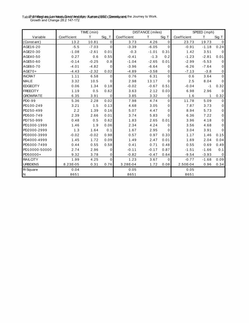
Table 3 shows the regression of density and other explanatory variables with
travel time, distance, and speed for automobile commuters. In this regression local
residential density is defined by a series of dummy [1,0] variables (PD0-99 to PD50000+)
indicating residence in a zip code in the respective density class, as shown in Table 2. Of
Published as: Levinson, David and Ajay Kumar (1997). Density and the Journey to Work. Growth and Change 28:2 147-172
these classes, PD7500-9999 is suppressed to more clearly demonstrate the automobile
travel time hypothesis. The results for trip distance and speed are as hypothesized: higher
density areas have slower speeds and shorter distances. As expected the relationship
between density and travel time requires some further discussion: generally travel time is
positively associated with density above 10,000 ppsm and negatively associated with
density below that 7,500 ppsm. Densities above 10,000 ppsm, and particularly over
50,000 ppsm, are observed primarily in older central cities, for instance New York
(discussed further in a later section), where diseconomies resulting from congestion may
exceed the advantage of higher accessibility. Below the 7,500 ppsm threshold, higher
residential density areas offer the advantage of better accessibility without as severe a
penalty in slower speeds, resulting in lower commuting time.
Urbanized area population density is positively associated with distance and not
statistically significant against time or speed. This tends to support the hypothesis that
metropolitan density is operating as a surrogate for city size. The number of edge cities,
representing the degree of polycentricity was not statistically significant. The rate of
growth, a measure of urban disequilibrium, was positively associated with travel time and
distance, though not speed. This corroborates the idea that high rates of change coupled
with relocation costs may prevent individuals from achieving their preferred bundle of
housing and travel choices.
The presence of heavy rail is positively associated with auto commuting time and
distance, and negatively associated with speed. The interesting part of this is not distance
or time, whose positive signs are in part a function of some autocorrelation between the
presence of rail and size of the city, but speed, which is lower for auto commuters in
cities with rail infrastructure, suggesting a possible investment effect. The proportion of
travel on freeways is positively associated with both distance and speed, and not
associated with time, suggesting the higher speeds are used to make longer distance
commutes, but not so far as to increase durations.
The socio-economic and demographic hypotheses were corroborated. The
regressions show that, for auto commuters, having a relatively high income, being a
male, and being a middle aged adult was positively associated with travel distance, speed,
and time. The longest times were found for adults in the suppressed category (age 30-40)
and the adjacent 40-50 year old category, as all others were negative relative to the
suppressed category. Distances were longest for the 30-40 year old group, while speeds
were highest for the 20-30 year olds.
Published as: Levinson, David and Ajay Kumar (1997). Density and the Journey to Work. Growth and Change 28:2 147-172
Transit Commuters: Nationally
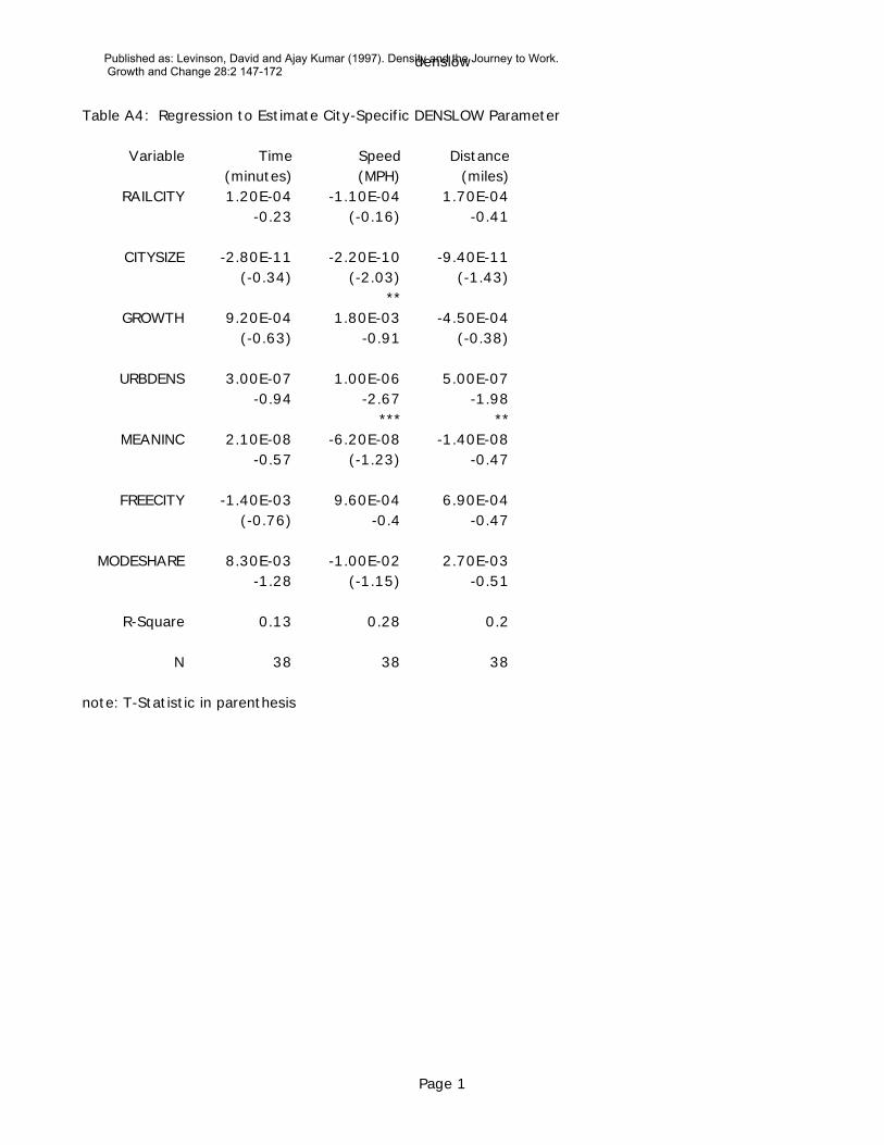
Table 4 shows the regression for transit users across the country. While in the
previous section we were able to use each density class as an independent variable,
because of the smaller sample of transit commuters, we had to aggregate the density
variable to attain meaningful results. Two continuous density variables are defined:
DENSLOW was set equal to the density for areas below 10,000 ppsm and was set equal
to zero for areas at or above 10,000 ppsm; and DENSHIGH was set equal to the density
at values of 10,000 ppsm and above, and was set equal to zero for areas below 10,000
ppsm. The 10,000 ppsm cut-off point was identified after a careful examination of the
data, and reflects the findings from the previous section. Although the exact inflection
point of the travel time vs. density relationship probably ranges somewhere between 7500
and 10,000 ppsm; the data classes recorded with the NPTS data prevent a finer analysis.
In contrast to auto commuters, transit users display a negative relationship
between travel time and density both above and below the 10,000 ppsm density
threshold, though the slope changes. Density is positively related to metropolitan
population, and bigger cities may be better served by transit facilities. Declining travel
times by transit and increasing travel times by auto as density rises above 10,000 ppsm
result in higher transit mode shares, as shown in Table 2.
The metropolitan density (URBDENS), principally a surrogate for city size, is
positively associated with time, distance, and speed, possibly because of higher rail
transit use. As with autos, the number of edge cities was not statistically significant.
However, unlike autos the growth rate was not statistically significant, perhaps because
of fairly low transit use in cities with high growth rates (typically sunbelt cities), and
particularly low transit use in the fastest growing (suburban) areas. Population growth
probably needs to be analyzed with changes in travel time using a longitudinal survey to
more fully understand its influence.
For transit commuters, time was positively associated with presence of heavy rail,
but distance and speed was not significant. In further analyses of transit, the impacts of
bus and of rail should be isolated. Freeway use is negatively related to speed and
distance, and again is not related to travel time. Freeways may be associated with bus use
as opposed to rail use for transit commuters, and again reflect the influence of
investment patterns and history on commuting behavior.
Income was associated with higher distances and speed, but the results for time
were not statistically significant. The question of whether high income persons who live
and work in the suburbs have shorter commutes than similarly situated lower income
Published as: Levinson, David and Ajay Kumar (1997). Density and the Journey to Work. Growth and Change 28:2 147-172
persons remains outstanding. For transit trips, adulthood has its expected influence
while, unlike for auto trips, gender is not statistically significant.
Automobile Commuters: City by City:
The NPTS database offers the possibility of analyzing the travel time relationship
for specific cities. Several cities augmented the sample size by contributing additional
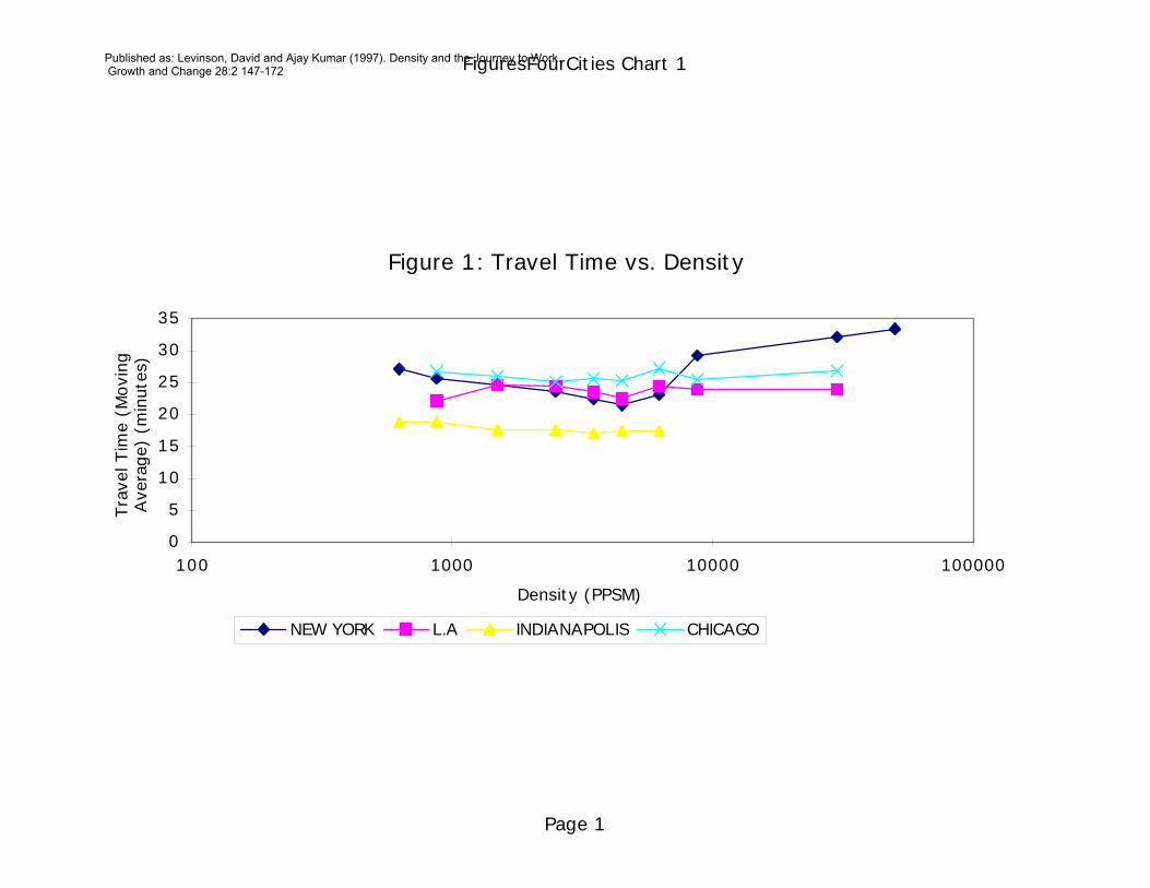
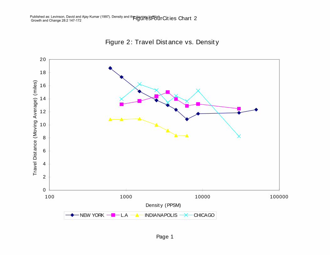
resources. Figure 1 shows residential density vs. travel time (by motorized modes) for
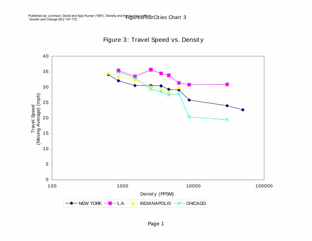
four cities (New York, Los Angeles, Chicago, and Indianapolis). Figures 2 and 3 show
density vs. distance and speed respectively. Travel time changes marginally with density
for each of the cities except New York. Indianapolis, the only city shown below 2
million population, has travel times one-third lower than the other three cities (each
above 8 million). Because sample sizes are low in density classes above 10,000 ppsm,
excepting New York, the relationship of high densities being positively associated with
travel time (discussed below) might only be found in cities of the size and density of New
York. We investigate this issue further.
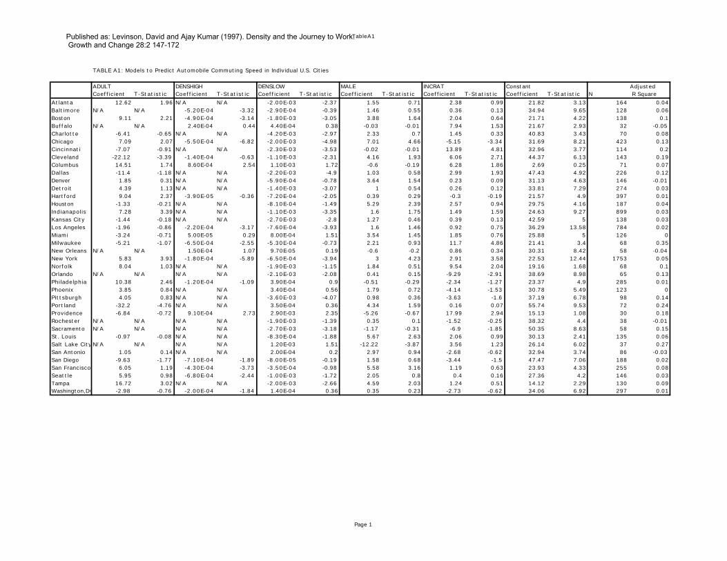
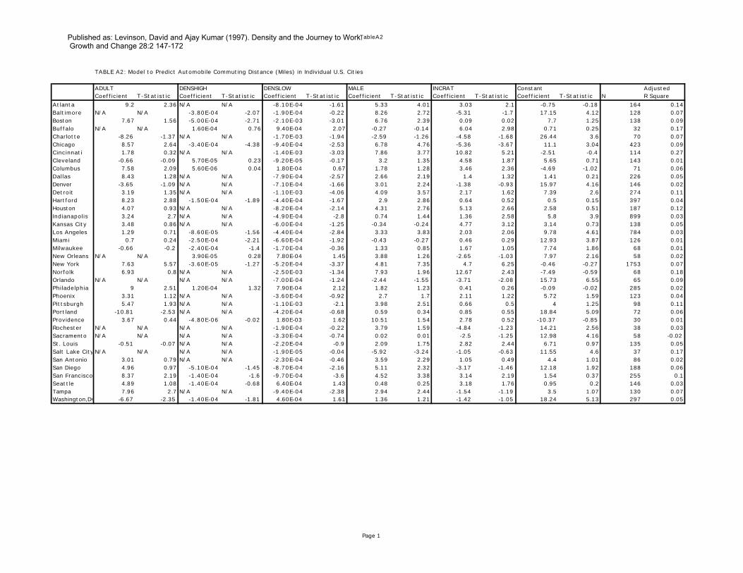
The previous section reviewed both inter- and intra- metropolitan variations in
travel time speed and distance using national data. However, we can eliminate the inter-
metropolitan variation by performing regressions on individual cities. Regressions were
conducted to predict travel speed, distance, and time for automobile commuters in each
of 38 specific cities using demographic (age, gender, income ratio) and density variables
as independent factors. As in the transit section, because of the small samples in each
density class in individual cities, we use the aggregate DENSLOW and DENSHIGH
variables. The key findings of the regressions are summarized in Charts 1-3, which
show the number of cities in which the hypotheses are corroborated, and the full tables
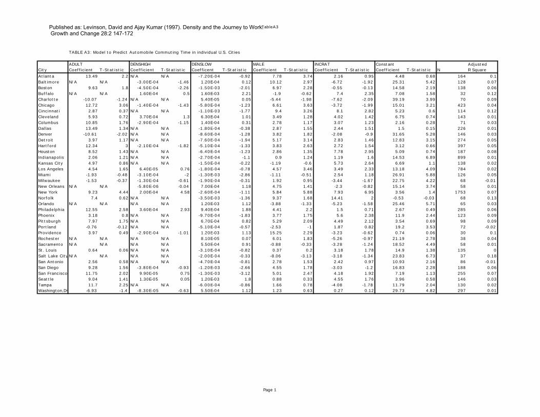
are given in the appendix (A1-A3).
The hypotheses for speed, time, and distance are shown below in Charts 1, 2, and
3, respectively where a “+” or “-“ reflect whether the relationships are expected to be
positive or negative. Then the number of cities where the results are positive and
significant at the 90% level or better, negative and significant, and not significant are
given.
Our general hypotheses for this section are confirmation of the results shown in
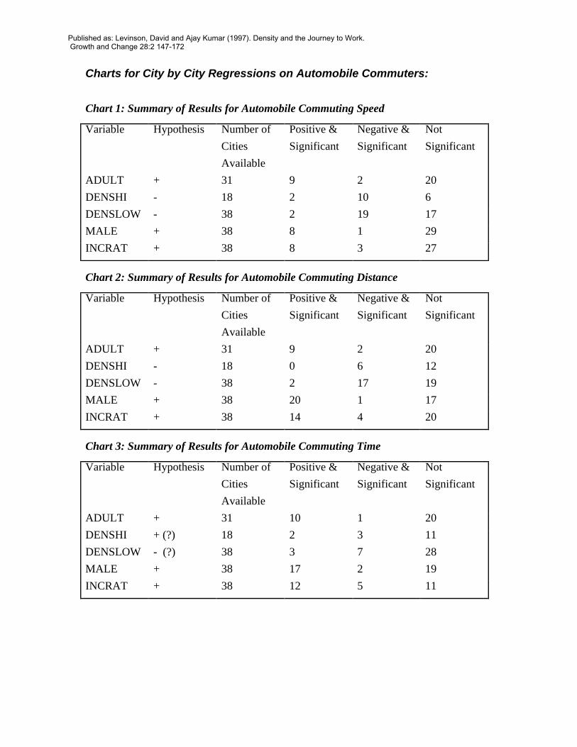
the previous section for the country as a whole. By and large, these are corroborated, as
seen in Chart 1. Residential density is clearly negatively associated with speed in most
cities at both high and low density levels. The two anomalies (in both low and high
Published as: Levinson, David and Ajay Kumar (1997). Density and the Journey to Work. Growth and Change 28:2 147-172
density categories) are Providence, Rhode Island and Columbus, Ohio, two of the
smallest cities in the analysis, both with small sample sizes.
The results for automobile commuting distance are shown in Chart 2. Density is
negatively correlated with commuting distance in almost all cases where significant
(Philadelphia and Buffalo excepted for low density areas). The national results are thus
in general corroborated.
Chart 3 shows the summary of the regressions to predict automobile commuting
time in each of 38 cities. The majority of the cities showed no significant relationship
between commuting time and density, at either low or high density, suggesting that speed
and distance are mostly off-setting. Where it was significant, the tendency was the higher
the density the lower the time for low density areas, corroborating the national results.
For high density areas, only 5 of 18 cases were significant, and they were split 3 negative,
2 positive, suggesting the need for more research.
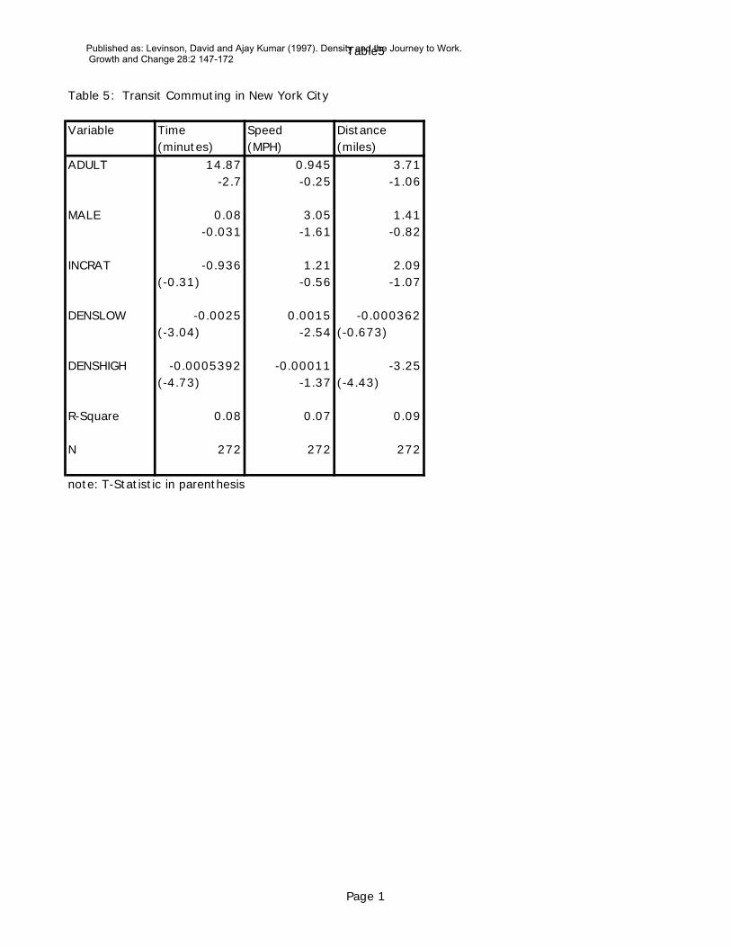
Transit Commuters in New York City
It would be desirable to analyze transit commuting in the same depth as auto
commuting, but the sample was too small in all cities but New York. Finally, table 5
shows the regressions to estimate speed, distance, and time for transit commuters in New
York, these are compared to the row of results in tables A1-A3 which looked at auto
commuters in New York. First speed: for New York’s auto commuters, the higher the
density the lower the speed, but for transit, just the opposite is true. Rail transit does not
suffer the same congestion problems as the automobile, and the higher density provides a
higher frequency of direct routes at least to 10,000 ppsm. Above that threshold, the effect
of density on speed is insignificant. These results differ from the national results for
transit, possibly due to New York’s exceptional dependence on rail.
Second, distance: for auto commuters density is negatively related to distance in
New York, this is true for transit commuters there too. This supports the national
findings. Finally, time: for auto commuters in New York, density is negatively related to
time up to 10,000 ppsm, and positively related above that value; however for the transit
commuter, density is negatively related to time at all densities. This confirms the
findings with the national data (including New York).
Published as: Levinson, David and Ajay Kumar (1997). Density and the Journey to Work. Growth and Change 28:2 147-172
SUMMARY AND CONCLUSIONS
This paper analyzes the magnitude and direction of the effects of residential
density and other variables concerning urban form on travel parameters after controlling
for demographic factors. It also reviews the relationship of density and demographics on
each of 38 specific cities. The investigation into the relationship between travel behavior
and density reveals some interesting results. While distance and speed are both
negatively associated with density, auto travel time is negatively related to density below
10,000 ppsm and positively related above 10,000 ppsm. The increase in travel time with
density above 10,000 ppsm indicates the possibility that beyond that threshold congestion
increases making driving a less attractive option. Transit users display a negative
relationship between travel time and density both above and below the 10,000 ppsm
density threshold. The declining transit time and increasing auto time above 10,000
ppsm explains the evidence of higher transit mode share in high density areas.
Metropolitan growth is found to be positively related to travel time for auto
commuters. This may indicate an inability of the public sector to provide transportation
infrastructure concurrently with population growth. The ability of households and firms
to mutually co-locate in growing suburbs with economies in travel time may, however,
involve some time lag which is not considered in this analysis.
Cities oriented around freeways have higher average speeds and distances, but no
significant relationship with time, reaffirming that individuals will adjust locations to take
advantage of higher speeds made available by freeways while maintaining travel time.
In addition, the presence of a rail system is associated with higher times and distances
for auto commuters and lower speeds, due perhaps to infrastructure investment patterns
or correlation between heavy rail and city size.
So we find that though density has noticeable effects on speed and distance of
trips, its effect on time is limited and contingent. A simple application of the standard
transportation-location tradeoff in urban economics might miss factors which temper the
importance of job markets on housing location and labor markets on firm location. For
individuals choosing a residence, their relevant accessibility includes factors other than
employment, such as access to family, schools, parks, shops, and the like. Household
location decisions are complicated by multiple workers for whom location needs to
considered. For firms choosing location, access to the labor market may offset access to
other firms. There are always lags in markets reaching “equilibrium” due to the
transaction costs of relocation. Finally, the increasing returns associated with continuing
physical placement in social and economic networks, such as the sunk nature of fixed
Published as: Levinson, David and Ajay Kumar (1997). Density and the Journey to Work. Growth and Change 28:2 147-172
costs in establishing contacts with friends, neighbors, business and colleagues, are
significant barriers to rapid relocation to shave a few minutes from a commute.
Use of these relationships for policy (for instance, to reduce the amount of
congestion, gasoline usage, or air pollution) must be tempered by several caveats. First,
the relationships of density cannot be isolated from self-selection bias. Individuals
choose a density (or distance from the center) based in part on how much they want to
commute and what lifestyle they wish to lead. Creating additional high density areas
may not increase the number of people with certain commuting and lifestyle preferences.
It certainly can’t be expected to increase the number of young singles or older retirees
who most often inhabit high density apartments. Second, these relationships are
particularly weak compared with total variation in commuting. Using density as a
primary tool influencing commuting behavior seems an expensive approach to the
problem. Third, though density is obviously associated with higher transit use, adding
development (upping density) increases the number of auto trips so long as auto mode
share is not zero, and in general, it is far from zero.
While density is an important explanatory variable, it is likely to be a much less
important policy instrument to influence commuting behavior. The ability of policy-
makers in relatively free markets to modify density are clearly marginal compared to the
size of cities, the area which is relevant when considering commuting and labor markets.
Furthermore, marginal changes in density are likely to have even more marginal changes
on commuting behavior. To be persuasive, arguments for higher density should rest on
stronger grounds than their impact on journey to work travel.
Published as: Levinson, David and Ajay Kumar (1997). Density and the Journey to Work. Growth and Change 28:2 147-172
ACKNOWLEDGMENTS
The authors would like to thank Susan Liss of the U.S. Department of Transportation for
providing the NPTS data. An earlier version of this paper was presented at the Western
Regional Science Association meeting in Napa, California (Feb 1996), the authors would
like to thank all who commented at the time, in particular Richard Crepeau. The authors
would also like to thank the staff of the Montgomery County Planning Department, and
the University of California at Berkeley. All errors, opinions, and analysis in the text
remain the responsibility of the authors.
END NOTE
1. While in general, highway and transit funding come from separate pots of money, the
Highway Act of 1973, and subsequent rules, allowed cities and states to trade money
earmarked from the Highway Trust Fund for construction of interstate highway
segments to general fund money used for transit (Smerk, 1991). More recently, the
Intermodal Surface Transportation Efficiency Act of 1991 has enabled a greater deal
of flexibility. To some extent, cities have had choices whether to invest in rail or
highways for over 20 years.
Published as: Levinson, David and Ajay Kumar (1997). Density and the Journey to Work. Growth and Change 28:2 147-172
REFERENCESBae, Chang-Hee Christine. 1993. Air Quality and Travel Behavior: Untying the Knot.
Journal of the American Planning Association. 59(1): 65-74.
Cervero, Robert. 1989. Jobs-Housing Balance and Regional Mobility. Journal of theAmerican Planning Association 55, 2: 136-50.
Dunphy, Robert T. and Kimberly Fisher. 1994. Transportation, Congestion, and Density:New Insights. Urban Land Institute. Washington DC
Frank, Lawrence D. and Gary Pivo. 1994. Impacts of Mixed Use and Density onUtilization of Three Modes of Travel: Single Occupant Vehicle, Transit andWalking. Transportation Research Record 1466 44-52
Garreau, Joel. 1991. Edge Cities: Life on the New Frontier. Doubleday. New York
Giuliano, Genevieve and Kenneth A. Small. 1991. “Subcenters in the Los AngelesRegion”. Regional Science and Urban Economics, 21, 163-82.
Giuliano, Genevieve and Kenneth A. Small. 1993. Is the Journey to Work Explained byUrban Structure?. Urban Studies . 30(9): 1485-1500
Goodwin, P. 1975. Variations in Travel Between Individuals Living in Areas of DifferentPopulation Density” Proceeding of a Seminar on Urban Traffic Models held on 7-11 July at the Planning and Transportation Research and Computation (PTRC)Summer Annual Meeting at the University of Warwick, England. London:Planning and Transport Research and Computation (International) (June)
Gordon P., H.W. Richardson, and H.L. Wong. 1986. The Distribution of Population andEmployment in a polycentric City: The Case of Los Angeles, Environment andPlanning A, 18, 161-173.
Gordon P., A. Kumar and H.W. Richardson. 1989a Congestion, Changing MetropolitanStructure and City Size in the U.S. International Regional Science Review 12,1:45-56
Gordon P., A. Kumar and H.W. Richardson. 1989b. The Influence of MetropolitanSpatial Structure on Commuting Times. Journal of Urban Economics 26: 138-49
Gordon P., A. Kumar and H.W. Richardson. 1989c. Gender Differences in MetropolitanTravel Behavior Regional Studies 23.6: 499-510
Greene, D. 1980. Recent Trends in Urban Spatial Structure, Growth and Change, 10, 29-40.
Handy, Susan. 1993. Regional versus Local Accessibility: Implications for Non-WorkTravel. presented at 72nd Annual Meeting of Transportation Research Board,Washington DC
Hanks, James W. and Timothy J. Lomax (1993) Roadway Congestion Estimates andTrends. Research Report 1131-4 Texas Transportation Institute July 1993
Heikkila, E. P. Gordon, J.I. Kim, R.B. Peiser, H.W. Richardson, and D. Dale-Johnson.1989. What Happened to the CBD-Distance Gradient?. Land Values in apolycentric City, Environment and Planning A 21, 221-232.
Isard, W. 1956. Location and Space Economy MIT Press, Cambridge, MA p.76
Levinson, David and Kumar, Ajay. 1995a. “A Multimodal Trip Distribution Model:Structure and Application.” Transportation Research Record # 1466, p 124-31
Published as: Levinson, David and Ajay Kumar (1997). Density and the Journey to Work. Growth and Change 28:2 147-172
Levinson David and Kumar, Ajay. 1995b. “Activity, Travel, and the Allocation of Time”Journal of the American Planning Association, Autumn 1995 61,4: 458-470
McDonald, John F. 1987. The Identification of Urban Employment Subcenters, Journalof Urban Economics, 21, 242-258.
McDonald, John F. and Paul Prather. 1994. Suburban Employment Centers: The Case ofChicago, Urban Studies, 31, 201-218.
Mills, Edwin S. 1972. Studies in the Structure of Urban Economy, Baltimore, JohnsHopkins 1972
Mitchelson, Ronald L. and James O. Wheeler. 1986. Analysis of Aggregate Flows: TheAtlanta Case. in The Geography of Urban Transportation, S. Hanson ed. GuilfordPress: New York.
Newman P.W.G. and J.R. Kenworthy. 1992. Is There a Role for Physical Planners?Journal of the American Planning Association 58, 3: 353-362
Pas, Eric I. 1980. Toward the understanding of urban travel behavior through theclassification of daily urban travel/activity patterns Dissertation: UMI- 81- 04755
Pushkarev, Boris and Jeffrey Zupan. 1977. Public Transportation and Land Use Policy,Bloomington Indiana, Indiana University Press
Richardson, H. 1973. The Economics of Urban Size, Saxon House, London
Scott, Allen J. .1988. Metropolis . University of California Press, Berkeley
Sivitanidou, Rena. 1995. Do Office Firms Value Access to Service Employment Centers?A Hedonic Value Analysis Within Polycentric Los Angeles? presented at 34thAnnual Meeting of the Western Regional Science Association San Diego, CAFeb. 22-26 1995
Steiner, Ruth. 1994. Residential Density and Travel Patterns: Review of the Literature.Transportation Research Record 1466 37-43.
Smerk, George M. (1991) The Federal Role in Urban Mass Transportation . IndianaUniversity Press, Bloomington Indiana
United States Bureau of Census (1984) “Population and Land Area of Urbanized Areasfor the United States and Puerto Rico” PC80-S1-14, Washington, DC
United States Bureau of Census (1991) “Census Press Release” 2.21.1991 CB91-66,Washington, DC
United States Department of Transportation (1990) Nationwide Personal TransportationSurvey, Washington, DC
Voorhees and Associates (1968) Factors and Trends in Trip Lengths, NationalCooperative Highway Research Report # 48, Washington DC
Published as: Levinson, David and Ajay Kumar (1997). Density and the Journey to Work. Growth and Change 28:2 147-172
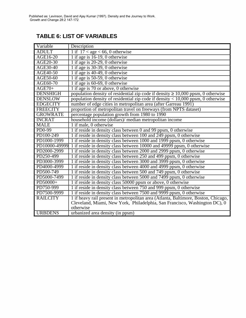
TABLE 6: LIST OF VARIABLES
Variable DescriptionADULT 1 if 17 < age < 66, 0 otherwiseAGE16-20 1 if age is 16-19, 0 otherwiseAGE20-30 1 if age is 20-29, 0 otherwiseAGE30-40 1 if age is 30-39, 0 otherwiseAGE40-50 1 if age is 40-49, 0 otherwiseAGE50-60 1 if age is 50-59, 0 otherwiseAGE60-70 1 if age is 60-69, 0 otherwiseAGE70+ 1 if age is 70 or above, 0 otherwiseDENSHIGH population density of residential zip code if density ≥ 10,000 ppsm, 0 otherwiseDENSLOW population density of residential zip code if density < 10,000 ppsm, 0 otherwiseEDGECITY number of edge cities in metropolitan area (after Garreau 1991)FREECITY proportion of metropolitan travel on freeways (from NPTS dataset)GROWRATE percentage population growth from 1980 to 1990INCRAT household income (dollars)/ median metropolitan incomeMALE 1 if male, 0 otherwisePD0-99 1 if reside in density class between 0 and 99 ppsm, 0 otherwisePD100-249 1 if reside in density class between 100 and 249 ppsm, 0 otherwisePD1000-1999 1 if reside in density class between 1000 and 1999 ppsm, 0 otherwisePD10000-49999 1 if reside in density class between 10000 and 49999 ppsm, 0 otherwisePD2000-2999 1 if reside in density class between 2000 and 2999 ppsm, 0 otherwisePD250-499 1 if reside in density class between 250 and 499 ppsm, 0 otherwisePD3000-3999 1 if reside in density class between 3000 and 3999 ppsm, 0 otherwisePD4000-4999 1 if reside in density class between 4000 and 4999 ppsm, 0 otherwisePD500-749 1 if reside in density class between 500 and 749 ppsm, 0 otherwisePD5000-7499 1 if reside in density class between 5000 and 7499 ppsm, 0 otherwisePD50000+ 1 if reside in density class 50000 ppsm or above, 0 otherwisePD750-999 1 if reside in density class between 750 and 999 ppsm, 0 otherwisePD7500-9999 1 if reside in density class between 7500 and 9999 ppsm, 0 otherwiseRAILCITY 1 if heavy rail present in metropolitan area (Atlanta, Baltimore, Boston, Chicago,
Cleveland, Miami, New York, Philadelphia, San Francisco, Washington DC), 0otherwise
URBDENS urbanized area density (in ppsm)
Published as: Levinson, David and Ajay Kumar (1997). Density and the Journey to Work. Growth and Change 28:2 147-172
Charts for City by City Regressions on Automobile Commuters:
Chart 1: Summary of Results for Automobile Commuting Speed
Variable Hypothesis Number of
Cities
Available
Positive &
Significant
Negative &
Significant
Not
Significant
ADULT + 31 9 2 20
DENSHI - 18 2 10 6
DENSLOW - 38 2 19 17
MALE + 38 8 1 29
INCRAT + 38 8 3 27
Chart 2: Summary of Results for Automobile Commuting Distance
Variable Hypothesis Number of
Cities
Available
Positive &
Significant
Negative &
Significant
Not
Significant
ADULT + 31 9 2 20
DENSHI - 18 0 6 12
DENSLOW - 38 2 17 19
MALE + 38 20 1 17
INCRAT + 38 14 4 20
Chart 3: Summary of Results for Automobile Commuting Time
Variable Hypothesis Number of
Cities
Available
Positive &
Significant
Negative &
Significant
Not
Significant
ADULT + 31 10 1 20
DENSHI + (?) 18 2 3 11
DENSLOW - (?) 38 3 7 28
MALE + 38 17 2 19
INCRAT + 38 12 5 11
Published as: Levinson, David and Ajay Kumar (1997). Density and the Journey to Work. Growth and Change 28:2 147-172
FiguresFourCities Chart 1
Page 1
Figure 1: Travel Time vs. Density
0
5
10
15
20
25
30
35
100 1000 10000 100000
Density (PPSM)
Tra
vel T
ime
(Mov
ing
Ave
rage
) (m
inut
es)
NEW YORK L.A INDIANAPOLIS CHICAGO
Published as: Levinson, David and Ajay Kumar (1997). Density and the Journey to Work. Growth and Change 28:2 147-172
FiguresFourCities Chart 2
Page 1
Figure 2: Travel Distance vs. Density
0
2
4
6
8
10
12
14
16
18
20
100 1000 10000 100000
Density (PPSM)
Tra
vel D
ista
nce
(Mov
ing
Ave
rage
) (m
iles)
NEW YORK L.A INDIANAPOLIS CHICAGO
Published as: Levinson, David and Ajay Kumar (1997). Density and the Journey to Work. Growth and Change 28:2 147-172
FiguresFourCities Chart 3
Page 1
Figure 3: Travel Speed vs. Density
0
5
10
15
20
25
30
35
40
100 1000 10000 100000
Density (PPSM)
Tra
vel S
peed
(M
ovin
g A
vera
ge)
(mph
)
NEW YORK L.A INDIANAPOLIS CHICAGO
Published as: Levinson, David and Ajay Kumar (1997). Density and the Journey to Work. Growth and Change 28:2 147-172
TABLE 1: TRANSPORTATION AND LAND USE VARIABLES FOR U.S. METROPOLITAN AREAS
source: (a) - 1980 U.S. Census, 1990 U.S. Census (b) - 1990/91 Nationwide Personal Transportation Survey
Published as: Levinson, David and Ajay Kumar (1997). Density and the Journey to Work. Growth and Change 28:2 147-172
Table 2: Transportation Variables by Density Class
Trip Frequency Auto Ownership Commuting Variables Commuting Mode Shares Mean Trips Mean Vehicles Mean Time by Mean Distance by Mean Speed by
Persons Per Sample Total Work Per Auto Transit Auto Transit Auto Transit Auto Transit Walk Square Mile Size Per Person HouseholdPerson (minutes) (miles) (miles per hour)