Density-functional theory in quantum chemistry
Trygve Helgaker
Centre for Theoretical and Computational Chemistry, University of Oslo, Norway
From Quarks to the Nuclear Many-Body Problem
A conference on recent advances in nuclear many-body physics
on the occasion of Eivind Osnes’ 70th birthday
Department of Physics, University of Oslo, Norway
May 21–24, 2008
1
Chemistry and mathematics
“Every attempt to employ mathematical methods in the study of
chemical questions must be considered profoundly irrational. If
mathematical analysis should ever hold a prominent place in chemistry—an
aberration which is happily impossible—it would occasion a rapid and
widespread degradation of that science.”
August Comte, 1798–1857
“The more progress sciences make, the more they tend to enter the
domain of mathematics, which is a kind of center to which they all converge.
We may even judge the degree of perfection to which a science has arrived by
the facility with which it may be submitted to calculation.”
Adolphe Quetelet, 1796–1874
— these different views are still with us today
2
Chemistry and physics
“The underlying physical laws necessary for the mathematical theory of a
large part of physics and the whole of chemistry are thus completely known,
and the difficulty is only that the exact application of these laws leads to
equations much too complicated to be soluble.”
P. A. M. Dirac
“All these [chemical] rules were ultimately explained in principle by
quantum mechanics, so that theoretical chemistry is in fact physics. On the
other hand, it must be emphasized that this explanation is in principle. We
have already discussed the difference between knowing the rules of the game
of chess, and being able to play.”
R. P. Feynman
— so, where are we today?
3
Quantum chemistry
• Chemical systems are difficult many-body problems
– with modern computers, the molecular many-body problem has become tractable
• Today, a large number of chemical problems have become amenable to calculation:
– molecular structure and spectroscopic constants
– reaction enthalpies and equilibrium constants
– reactivity, reaction rates, and dynamics
– interaction with applied electromagnetic fields and radiation
• Nowadays, quantum-chemical calculations are routinely carried out by nonspecialists:
– computation constitutes about one quarter of all chemical research
– we are number crunchers
• Quantum chemistry has been responsible for many qualitative models in chemistry
– such models are good and useful
– however, they do not constitute the bread and butter of quantum chemistry
• Quantum chemists must provide tools that compete with experiment
– ideally, our results should be as accurate as experiment: chemical accuracy
– if we cannot consistently provide high accuracy, we will be out of business
4
History of quantum chemistry
• Quantum mechanics has been applied to chemistry since the 1920s
– early accurate work on He and H2
– semi-empirical applications to larger molecules
• An important development was that of ab initio theory
– Hartree–Fock (HF) self-consistent field (SCF) theory (1960s)
– configuration-interaction (CI) theory (1970s)
– multiconfigurational SCF (MCSCF) theory (early 1980s)
– many-body perturbation theory (1980s)
– coupled-cluster theory (late 1980s)
• Coupled-cluster theory is the most successful wave-function theory
– introduced from nuclear physics
– size extensive
– hierarchical
– the exact solution can be approached in systematic manner
– high cost, near-degeneracy problems
• Density-functional theory (DFT) emerged during the 1990s
5
Coupled-cluster theory
• In coupled-cluster (CC) theory, the starting point is the HF description
• This description is improved upon by the application of excitation operators
|CC〉 =“
1 + Xai
”
| {z }
singles
· · ·“
1 + Xabij
”
| {z }
doubles
· · ·“
1 + Xabcijk
”
| {z }
triples
· · ·“
1 + Xabcdijkl
”
| {z }
quadruples
· · · |HF〉
– with each virtual excitation, there is an associated probability amplitude tabc···ijk···
– single excitations represent orbital adjustments rather than interactions
– double excitations are particularly important, arising from pair interactions
– higher excitations should become progressively less important
• This classification provides a hierarchy of ‘truncated’ CC wave functions:
– CCS, CCSD, CCSDT, CCSDTQ, CCSDTQ5, . . .
• The quality of the calculation also depends on the size of the virtual space
– cc-pVDZ, cc-pVTZ, cc-pVQZ, cc-pVTZ, cc-pV6Z, . . .
– each new level introduces a new shell of orbitals of each angular momentum
– the orbitals are expanded in nuclear-fixed Gaussians
6
The two-dimensional chart of quantum chemistry
• The quality of ab initio calculations is determined by the description of
1. the N -electron space (wave-function model);
2. the one-electron space (basis set).
• Normal distributions of errors in AEs (kJ/mol)
-200 200
HFDZ
-200 200 -200 200
HFTZ
-200 200 -200 200
HFQZ
-200 200 -200 200
HF5Z
-200 200 -200 200
HF6Z
-200 200
-200 200
MP2DZ
-200 200 -200 200
MP2TZ
-200 200 -200 200
MP2QZ
-200 200 -200 200
MP25Z
-200 200 -200 200
MP26Z
-200 200
-200 200
CCSDDZ
-200 200 -200 200
CCSDTZ
-200 200 -200 200
CCSDQZ
-200 200 -200 200
CCSD5Z
-200 200 -200 200
CCSD6Z
-200 200
-200 200
CCSD(T)DZ
-200 200 -200 200
CCSD(T)TZ
-200 200 -200 200
CCSD(T)QZ
-200 200 -200 200
CCSD(T)5Z
-200 200 -200 200
CCSD(T)6Z
-200 200
• The errors are systematically reduced by going up in the hierarchies
7
Energy contributions to atomization energies (kJ/mol)
• Contributions of each CC excitation level (left) and AO basis-set shell (right)
HF CCSD CCSDT CCSDTQ
1
10
100
1000
Log-Lin
DZ TZ QZ 5Z 6Z
1
10
100
1000Log-Log
– color code: HF , N2 , F2 , and CO
• The excitation-level convergence is approximately linear (log–linear plot)
– each new excitation level reduces the error by about an order of magnitude
– the contributions from quintuples are negligible (about 0.1 kJ/mol)
• The basis-set convergence is much slower (log–log plot)
– each shell contributes an energy proportional to X−4 where X is the cardinal number
– a similarly small error (0.1 kJ/mol) requires X > 10
– clearly, we must choose our orbitals in the best possible manner
8
CC convergence: bond distances (pm)
RHF SD T Q 5 rel. theory exp. err.
HF 89.70 1.67 0.29 0.02 0.00 0.01 91.69 91.69 0.00
N2 106.54 2.40 0.67 0.14 0.03 0.00 109.78 109.77 0.01
F2 132.64 6.04 2.02 0.44 0.03 0.05 141.22 141.27 −0.05
CO 110.18 1.87 0.75 0.04 0.00 0.00 112.84 112.84 0.00
CC convergence: harmonic constants ωe (cm−1)
RHF SD T Q 5 rel. theory exp. err.
HF 4473.8 −277.4 −50.2 −4.1 −0.1 −3.5 4138.5 4138.3 0.2
N2 2730.3 −275.8 −72.4 −18.8 −3.9 −1.4 2358.0 2358.6 −0.6
F2 1266.9 −236.1 −95.3 −15.3 −0.8 −0.5 918.9 916.6 2.3
CO 2426.7 −177.4 −71.7 −7.2 0.0 −1.3 2169.1 2169.8 0.7
9
Convergence to ωe in N2
371.9
84.6
4.113.8
23.54.7 0.8
HF CCSD�FC CCSDHTL�FC CCSDHTL CCSDT CCSDTQ CCSDTQ5
10
The emergence of DFT
• The traditional methods of quantum chemistry are capable of high accuracy
– nevertheless, most calculations are performed using density-functional theory (DFT)
• What is the reason for the popularity of DFT?
– the standard methods are (at least for high accuracy) very expensive
11
Density-functional theory
• For chemists, we view the electronic energy as a functional E[v] of the potential
v(r) =P
KZKrK
Coulomb potential
• In standard QC, we determine E[v] by solving (approximately) the Schrodinger equation
E[v] = minΨ〈Ψ|H[v]|Ψ〉 variation principle
• However, the negative ground-state energy E[v] is a convex functional of the potential
E(cv1 + (1− c)v2) ≥ cE(v1) + (1− c)E(v2), 0 ≤ c ≤ 1 convexity
x1 x2
fHx1L
fHx2L
c fHx1L+H1-cL fHx2L
fHx2L
c x1+H1-cLx2
fHc x1+H1-cLx2L
• The energy may then be expressed in terms of its Legendre–Fenchel transform
F [ρ] = supv
`E[v]−
Rv(r)ρ(r) dr
´energy as a functional of density
E[v] = infρ
`F [ρ] +
Rv(r)ρ(r) dr
´energy as a functional of potential
– the universal density functional F [ρ] is the central quantity in DFT
12
The conjugate energy functionals E[v] and F [ρ]
• As chemists we may choose to work in terms of E[v] or F [ρ]:
F [ρ] = supv
`E[v]−
Rv(r)ρ(r) dr
´definition of the universal density functional
E[v] = infρ
`F [ρ] +
Rv(r)ρ(r) dr
´Hohenberg–Kohn variation principle
• The potential v(r) and the density ρ(r) are conjugate variables
– they belong to dual linear spaces such thatR
v(r)ρ(r) dr is finite
– they satisfy the reciprocal relations
δF [ρ]/δρ(r) = −v(r), δE[v]/δv(r) = ρ(r)
• In molecular mechanics (MM), we work in terms of E[v]
– parametrization of energy as a function of bond distances, angles etc.
– widely used for large systems (in biochemistry)
• In density-functional theory (DFT), we work in terms of F [ρ]
– the exact functional is unknown but useful approximations exist
– more accurate the molecular mechanics, widely used in chemistry
• Neither method involves the direct solution of the Schrodinger equation
13
Kohn–Sham theory
• The Hohenberg–Kohn variation principle
E[v] = min ρ`F [ρ] +
Rv(r)ρ(r) dr
´
– the functional form of F [ρ] is unknown—the kinetic energy is most difficult
• A noninteracting system can be solved exactly, at low cost, by introducing orbitals
F [ρ] = Ts[ρ] + J [ρ] + Exc[ρ], ρ(r) =P
i φi(r)∗φi(r)
where the contributions are
Ts[ρ] = − 12
P
i
Rφ∗
i (r)∇2φi(r)dr noninteracting kinetic energy
J [ρ] =
ZZ
ρ(r1)ρ(r2)r−112 dr1dr2 Coulomb energy
Exc[ρ] = F [ρ]− Ts[ρ]− J [ρ] exchange–correlation energy
• In Kohn–Sham theory, we solve a noninteracting problem in an effective potential
ˆ− 1
2∇2 + veff(r)
˜φi(r) = εiφi(r), veff(r) = v(r) + vJ(r) +
δExc[ρ]δρ(r)
– veff(r) is adjusted such that the noninteracting density is equal to the true density
– it remains to specify the exchange–correlation functional Exc[ρ]
14
The exchange–correlation functional
• The exact exchange–correlation functional is unknown
– we must rely on approximations
• Local-density approximation (LDA)
– XC functional modeled after the uniform electron gas (which is known exactly)
ELDAxc [ρ] =
Z
f(ρ(r)) dr local dependence on density
– widely applied in condensed-matter physics
– not sufficiently accurate to compete with traditional methods of quantum chemistry
• Generalized-gradient approximation (GGA)
– introduce a dependence also on the density gradient
EGGAxc [ρ] =
Z
f(ρ(r, ∇ρ(r)) dr local dependence on density and its gradient
– Becke’s gradient correction to exchange (1988) changed the situation
– the accuracy became sufficient to compete in chemistry
– indeed, surprisingly high accuracy for energetics
15
Exchange–correlation functionals (plural)
• The exchange–correlation energy contains several contributions
Exc[ρ] = F [ρ]− Ts[ρ]− J [ρ]
– exchange (dominant), correlation, kinetic-energy correction
• The Dirac exchange with Becke’s gradient correction:
EX =P
σ
Rρσ
`EDirac
σ (r) + EBeckeσ (r)
´dr
EDiracσ (r) = − 3
4
`6π
´1/3ρ1/3σ (r)
EBeckeσ (r) = −
βρ1/3σ (r)s2
σ(r)
1+6βsσ(r) sinh−1 sσ(r), sσ(r) =
|∇ρσ(r)|
ρ4/3σ (r)
– the Becke correction contains the adjustable parameter β = 0.0042
– fitted to HF exchange of noble-gas atoms
• The Becke correction is often used with the LYP (Lee–Yang–Parr) correlation functional
– contains four adjustable parameters, fitted to the helium-atom correlation energy
• The resulting functional is known under the acronym BLYP
– a bewildering variety of functionals has been developed
– sometimes chosen to satisfy exact conditions, other times fitted to data
16
Hybrid DFT
• We have already introduced orbitals to evaluate the kinetic energy
– why not use the orbitals to evaluate the exact HF exchange?
– this is both a good and bad idea . . .
• The replacement of functional exchange with exact exchange makes things worse
– at least for energetics...
– it is difficult to find a correlation functional to match exact exchange
– this has to do with the delocalization of the exact exchange hole
• However, some proportion of exact exchange is a good thing for energetics
– in B3LYP, 20% is used: good for energetics
– this has for many years been the most popular functional
• For other properties, 100% exact exchange is better. . .
– polarizabilities, excitation energies
• Attempts have been made to use orbitals in a variety of manners
– dispersion is not described by local and semi-local functionals
– traditional quantum chemistry describes dispersion well
– elements of MP2 introduced into DFT
17
A plethora of exchange–correlation functionals
Table 1. MADs (all energies in eV) for various level of theory for the extended G2 set
Method
G2(MAD)
H-Ne, Etot TM �E He2, �E(Re) Ne2, �E(Re) (H2O)2, De(RO . . . O)�Hf IP EA PA
HF 6.47 1.036 1.158 0.15 4.49 1.09 Unbound Unbound 0.161 (3.048)
G2 or best ab initio 0.07a 0.053b 0.057b 0.05b 1.59c 0.19d 0.0011 (2.993)e 0.0043 (3.125)e 0.218 (2.912)f
LDA (SVWN) 3.94a 0.665 0.749 0.27 6.67 0.54g 0.0109 (2.377) 0.0231 (2.595) 0.391 (2.710)
GGA
BP86 0.88a 0.175 0.212 0.05 0.19 0.46 Unbound Unbound 0.194 (2.889)
BLYP 0.31a 0.187 0.106 0.08 0.19 0.37g Unbound Unbound 0.181 (2.952)
BPW91 0.34a 0.163 0.094 0.05 0.16 0.60 Unbound Unbound 0.156 (2.946)
PW91PW91 0.77 0.164 0.141 0.06 0.35 0.52 0.0100 (2.645) 0.0137 (3.016) 0.235 (2.886)
mPWPWh 0.65 0.161 0.122 0.05 0.16 0.38 0.0052 (2.823) 0.0076 (3.178) 0.194 (2.911)
PBEPBEi 0.74i 0.156 0.101 0.06 1.25 0.34 0.0032 (2.752) 0.0048 (3.097) 0.222 (2.899)
XLYPj 0.33 0.186 0.117 0.09 0.95 0.24 0.0010 (2.805) 0.0030 (3.126) 0.192 (2.953)
Hybrid methods
BH & HLYPk 0.94 0.207 0.247 0.07 0.08 0.72 Unbound Unbound 0.214 (2.905)
B3P86l 0.78a 0.636 0.593 0.03 2.80 0.34 Unbound Unbound 0.206 (2.878)
B3LYPm 0.13a 0.168 0.103 0.06 0.38 0.25g Unbound Unbound 0.198 (2.926)
B3PW91n 0.15a 0.161 0.100 0.03 0.24 0.38 Unbound Unbound 0.175 (2.923)
PW1PWo 0.23 0.160 0.114 0.04 0.30 0.30 0.0066 (2.660) 0.0095 (3.003) 0.227 (2.884)
mPW1PWp 0.17 0.160 0.118 0.04 0.16 0.31 0.0020 (3.052) 0.0023 (3.254) 0.199 (2.898)
PBE1PBEq 0.21i 0.162 0.126 0.04 1.09 0.30 0.0018 (2.818) 0.0026 (3.118) 0.216 (2.896)
O3LYPr 0.18 0.139 0.107 0.05 0.06 0.49 0.0031 (2.860) 0.0047 (3.225) 0.139 (3.095)
X3LYPs 0.12 0.154 0.087 0.07 0.11 0.22 0.0010 (2.726) 0.0028 (2.904) 0.216 (2.908)
Experimental — — — — — — 0.0010 (2.970)t 0.0036 (3.091)t 0.236u (2.948)v
�Hf, heat of formation at 298 K; PA, proton affinity; Etot, total energies (H-Ne); TM �E, s to d excitation energy of nine first-row transition metal atoms and
nine positive ions. Bonding properties [�E or De in eV and (Re) inÅ] are given for He2, Ne2, and (H2O)2. The best DFT results are in boldface, as are the most accurate
answers [experiment except for (H2O)2].aRef. 5.
18
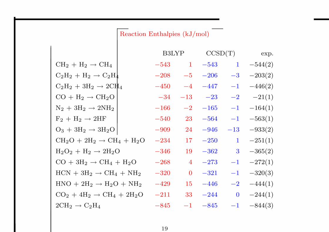
Reaction Enthalpies (kJ/mol)
B3LYP CCSD(T) exp.
CH2 + H2 → CH4 −543 1 −543 1 −544(2)
C2H2 + H2 → C2H4 −208 −5 −206 −3 −203(2)
C2H2 + 3H2 → 2CH4 −450 −4 −447 −1 −446(2)
CO + H2 → CH2O −34 −13 −23 −2 −21(1)
N2 + 3H2 → 2NH2 −166 −2 −165 −1 −164(1)
F2 + H2 → 2HF −540 23 −564 −1 −563(1)
O3 + 3H2 → 3H2O −909 24 −946 −13 −933(2)
CH2O + 2H2 → CH4 + H2O −234 17 −250 1 −251(1)
H2O2 + H2 → 2H2O −346 19 −362 3 −365(2)
CO + 3H2 → CH4 + H2O −268 4 −273 −1 −272(1)
HCN + 3H2 → CH4 + NH2 −320 0 −321 −1 −320(3)
HNO + 2H2 → H2O + NH2 −429 15 −446 −2 −444(1)
CO2 + 4H2 → CH4 + 2H2O −211 33 −244 0 −244(1)
2CH2 → C2H4 −845 −1 −845 −1 −844(3)
19
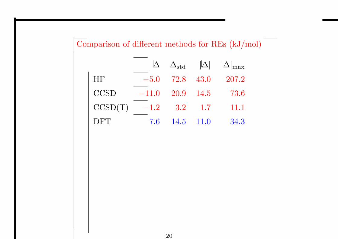
Comparison of different methods for REs (kJ/mol)
∆ ∆std |∆| |∆|max
HF −5.0 72.8 43.0 207.2
CCSD −11.0 20.9 14.5 73.6
CCSD(T) −1.2 3.2 1.7 11.1
DFT 7.6 14.5 11.0 34.3
20
Molecular properties
• Over the last decade, DFT has become the workhorse of chemistry
– its popularity stems from its ability to provide good structures and energetics
• DFT is widely used also for molecular properties
– response theory
– geometric, electric, magnetic perturbations
– static and dynamic perturbations
– linear and nonlinear response
• For most properties, the application of DFT has been a success
– a revolution in the calculation of nuclear spin–spin coupling constants
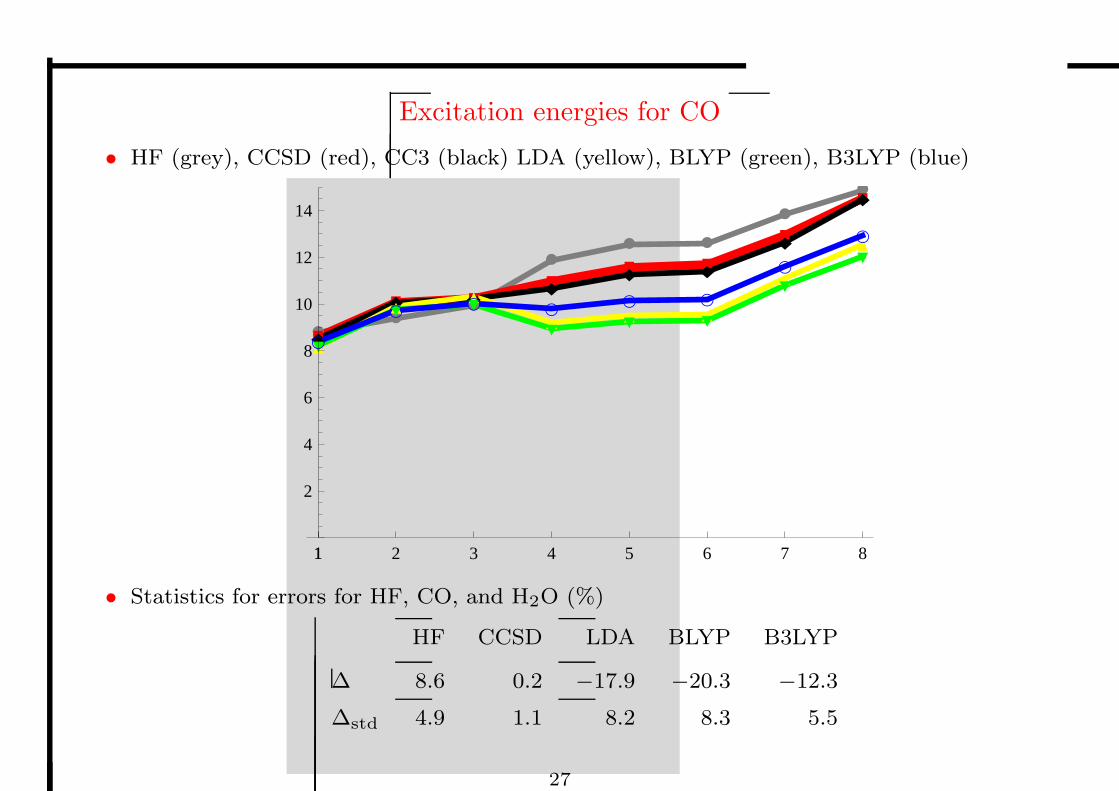
• Excitation energies are an interesting case
– important chemical property of molecules
– accessible from linear-response theory
– some excitations are well reproduced, others poorly
– the failures highlight deficiencies in the exchange–correlation potential
21
Response theory
• The expectation value of A in the presence of a perturbation Vω of frequency ω:
˙t˛˛A
˛˛t
¸=
˙0
˛˛A
˛˛0
¸+
Z
〈〈A; Vω〉〉ω exp (−iωt) dω + · · ·
– the linear-response function 〈〈A; Vω〉〉ω carries information about the first-order
change in the expectation value
• The linear-response function may be represented compactly as:
〈〈A; V ω〉〉ω = −A[1]T
`E
[2] − ωS[2]
´−1
V[1]ω
| {z }
linear equations
←
8><
>:
E[2] electronic Hessian
S[2] metric matrix
A[1] = vec
`
ADS − SDA´
• In practice, the response functions are evaluated by solving a set of linear equations
`E
[2] − ωS[2]
´N
[1] = −V[1]ω
〈〈A; V ω〉〉ω = A[1]T
N[1]
• Excitation energies as poles of linear response function (RPA):
`E
[2] − ωS[2]
´X = 0
22
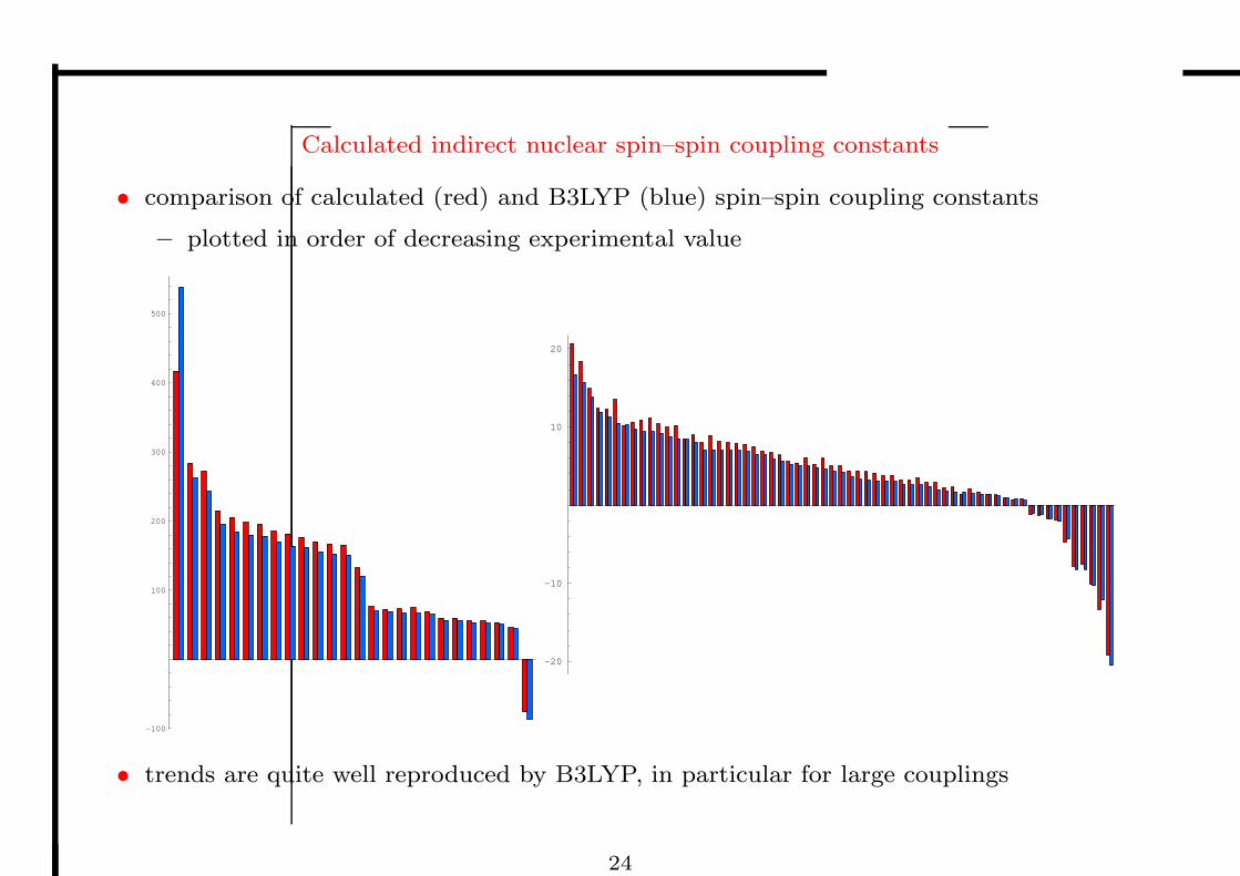
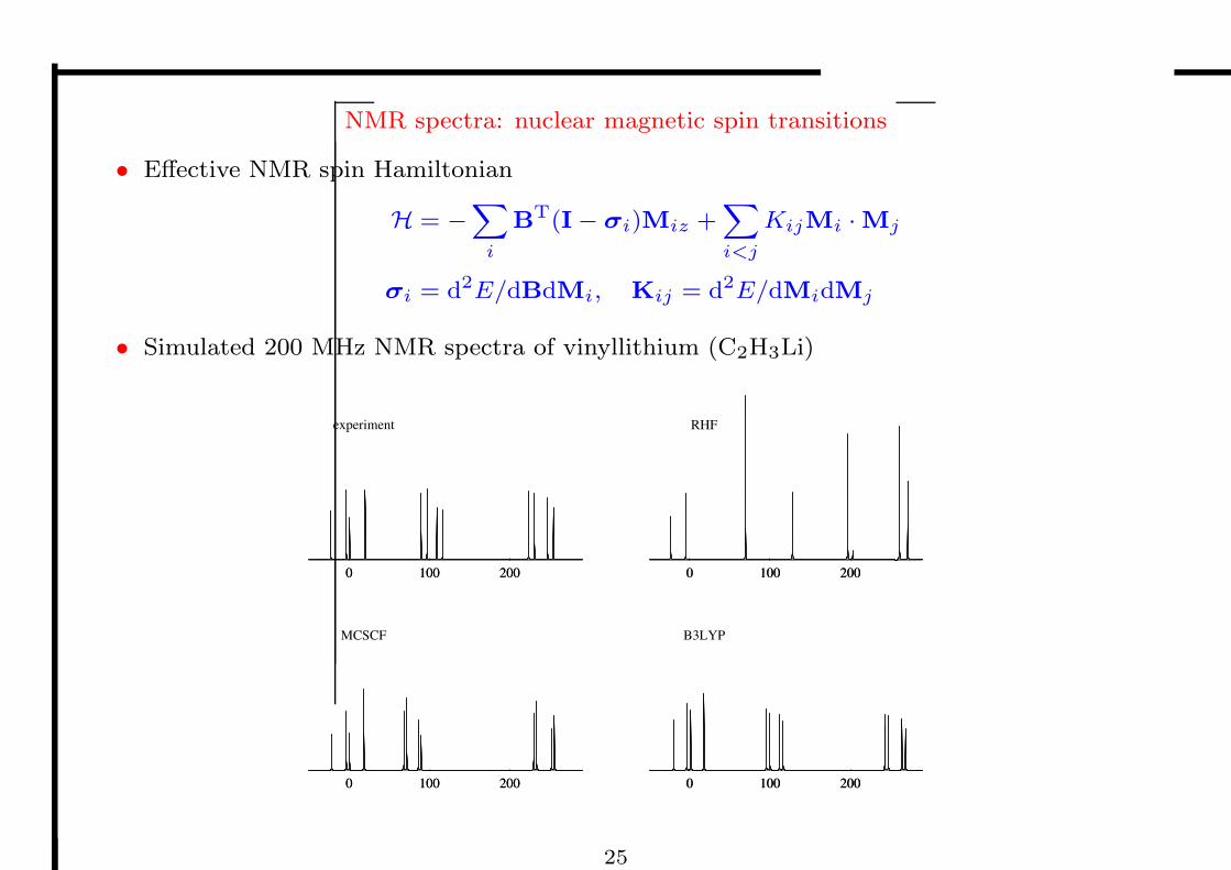
Indirect nuclear spin–spin coupling constants
• With each nucleus in a molecule, there is an associated magnetic moment MP :
– their direct interactions vanish in isotropic media
– the residual indirect interaction arises from hyperfine
interactions with the electrons ≈ 10−16Eh ≈ 1 Hz
• The indirect nuclear spin–spin coupling constants are calculated as the second
derivatives of the total electronic energy (i.e., by linear response theory)
– for each nucleus, 3 singlet and 7 triplet response equations are solved
• The introduction of DFT has created something of revolution in the calculation of
spin–spin coupling constants, greatly expanding the application range of theory
• The accuracy of DFT is similar to that of wave-function theory:
-30 30
CAS
-30 30 -30 30
RAS
-30 30 -30 30
SOPPA
-30 30 -30 30
CCSD
-30 30
-30 30
HF
-30 30
LDA
-30 30 -30 30
BLYP
-30 30 -30 30
B3LYP
-30 30
23
Calculated indirect nuclear spin–spin coupling constants
• comparison of calculated (red) and B3LYP (blue) spin–spin coupling constants
– plotted in order of decreasing experimental value
-100
100
200
300
400
500
-20
-10
10
20
• trends are quite well reproduced by B3LYP, in particular for large couplings
24
NMR spectra: nuclear magnetic spin transitions
• Effective NMR spin Hamiltonian
H = −X
i
BT(I− σi)Miz +
X
i<j
KijMi ·Mj
σi = d2E/dBdMi, Kij = d2E/dMidMj
• Simulated 200 MHz NMR spectra of vinyllithium (C2H3Li)
0 100 200
MCSCF
0 100 200 0 100 200
B3LYP
0 100 200
0 100 200
experiment
0 100 200 0 100 200
RHF
0 100 200
25
Valinomycin C54H90N8O18
• DFT can be applied to large molecular systems such as valinomycin (168 atoms)
– there are a total of 7587 spin–spin couplings to the carbon atoms in valinomycin
– below, we have plotted the magnitude of the reduced LDA/6-31G coupling constants
on a logarithmic scale, as a function of the internuclear distance:
500 1000 1500
1019
1016
1013
– the coupling constants decay in characteristic fashion, which we shall examine
– most of the indirect couplings beyond 500 pm are small and cannot be detected
26
Excitation energies for CO
• HF (grey), CCSD (red), CC3 (black) LDA (yellow), BLYP (green), B3LYP (blue)
ææ
æ
æ
æ æ
æ
æ
à
à à
à
à à
à
à
ì
ì ìì
ì ì
ì
ì
ò
òò
òò ò
ò
ò
ô
ô ô
ôô ô
ô
ô
ç
çç ç
ç ç
ç
ç
11 2 3 4 5 6 7 8
2
4
6
8
10
12
14
• Statistics for errors for HF, CO, and H2O (%)
HF CCSD LDA BLYP B3LYP
∆ 8.6 0.2 −17.9 −20.3 −12.3
∆std 4.9 1.1 8.2 8.3 5.5
27
Deficiencies of DFT excitation energies
• DFT represents local excitations well
– excitations to outer valence and charge-transfer (CT) excitations less well described
– the potential falls off too fast—the asymptotic behaviour should be
limr→∞
vxc(r) = −1
r
• This can be corrected by the inclusion of exact exchange
– exact exchange can be introduced in different manners
2 4 6 8
0.2
0.4
0.6
0.8
1.0HF
B3LYP
CAM-B3LYP
LC
– the proportion of exact exchange as a function of r
28
Tripeptide excitations
N
N
O
H
N
O
OH
H
excitation type PBE B3LYP CAM exp.
n2 → π∗
2 local 5.58 5.74 5.92 5.61
n1 → π∗
1 local 5.36 5.57 5.72 5.74
n3 → π∗
3 local 5.74 5.88 6.00 5.91
π1 → π∗
2 CT 5.18 6.27 6.98 7.01
π2 → π∗
3 CT 5.51 6.60 7.68 7.39
n1 → π∗
2 CT 4.61 6.33 7.78 8.12
n2 → π∗
3 CT 5.16 6.83 8.25 8.33
π1 → π∗
3 CT 4.76 6.06 8.51 8.74
n1 → π∗
3 CT 4.26 6.12 8.67 9.30
29
Excitation energies against Λ for PBE
• With this GGA functional, performance for Λ < 0.6 is erratic
• local excitations (Λ > 0.4) are well reproduced, within a few tenths of an eV
• Rydberg excitations (Λ < 0.3) are systematically underestimated by a few eVs
• CT excitations cover a surprisingly large Λ range (DMABN)
30
Excitation energies against Λ for B3LYP
• With the introduction of exact exchange, performance improves
• local excitations are lifted and cover a slightly larger Λ range
• errors in Rydberg excitations are reduced by a factor of two
• likewise, an improvement in CT excitations is observed
31
Excitation energies against Λ for CAM-B3LYP
• Coulomb attenuation gives a uniform description of local and nonlocal excitations!
– however, errors as large as 1 eV are still observed
32
The importance of exact exchange for longitudinal polarizabilities
• Without a good description of long-range exchange, the systems become too polarizable
50 100 150 200 250 300 350
100
200
300
400
500
600
LDA H0%L
BLYP H0%L
B3LYP H20%L
CAM-B3LYP H19%®65%L
HF H100%L CAM-B3LYP+ H19%®100%L
Hartree H0%L
– the Hartree model neglects all exchange and overestimates by a factor of eight
– pure DFT has a poor long-range exchange and overestimates by a factor of four
– hybrid functionals improve the situation, introducing some exact exchange
– compromise solution: standard DFT at short range, full exchange at long range
33
Conclusions
• Quantum chemistry has emerged as an important part of chemistry
• Since the 1920s, a large number of techniques have been developed
– wave-function construction (ab initio)
– density-functional theory (DFT)
– molecular mechanics (MM)
• The wave-function methods offer high accuracy and error control
– can be systematically improved towards the exact solution
– high cost but progress towards low cost based on locality
– necessary for benchmarking
• DFT is nowadays the workhorse of quantum chemistry
– low cost and reasonable accuracy but cannot be systematically improved
– often used in conjunction with wave-function methods
• Large systems are treated using MM techniques
– combined quantum-mechanics/molecular-mechanis (QM/MM) methods
34