DEPARTMENT OF DEFENSE HANDBOOK - …statisticalengineering.com/mh1823/MIL-HDBK-1823A(2009).pdf ·...

NOT MEASUREMENT SENSITIVE

MIL-HDBK-1823A 7 April 2009 ————————— SUPERSEDING MIL-HDBK-1823 14 April 2004

DEPARTMENT OF DEFENSE HANDBOOK

NONDESTRUCTIVE EVALUATION SYSTEM RELIABILITY ASSESSMENT

This handbook is for guidance only. Do not cite this document as a requirement.

AMSC N/A AREA NDTI DISTRIBUTION STATEMENT A. Approved for public release; distribution is unlimited.

MIL-HDBK-1823A

2

FOREWORD

1. This handbook is approved for use by all Departments and Agencies of the Department of Defense.

2. This handbook is for guidance only and cannot be cited as a requirement. If it is, the contractor does not have to comply.

3. Comments, suggestions, or questions on this document should be addressed to ASC/ENRS, 2530 Loop Road West, Wright-Patterson AFB 45433-7101, or emailed to [email protected]. Since contact information can change, you may want to verify the currency of this address information using the ASSIST Online database at http://assist.daps.dla.mil.

mailto:[email protected]�

http://assist.daps.dla.mil/�

MIL-HDBK-1823A

CONTENTS PARAGRAPH PAGE

3

1. SCOPE .............................................................................................................................. 13 1.1 Scope ................................................................................................................................. 13 1.2 Limitations ........................................................................................................................ 13 1.3 Classification .................................................................................................................... 13 2. APPLICABLE DOCUMENTS ........................................................................................ 14 2.1 General .............................................................................................................................. 14 2.2 Non-Government publications .......................................................................................... 14 3. Nomenclature .................................................................................................................... 15 4. GENERAL GUIDANCE .................................................................................................. 21 4.1 General .............................................................................................................................. 21 4.2 System definition and control ........................................................................................... 21 4.3 Calibration ........................................................................................................................ 21 4.4 Noise ................................................................................................................................. 21 4.5 Demonstration design ....................................................................................................... 21 4.5.1 Experimental design ......................................................................................................... 21 4.5.1.1 Test variables .................................................................................................................... 22 4.5.1.2 Test matrix ........................................................................................................................ 24 4.5.2 Test specimens .................................................................................................................. 25 4.5.2.1 Physical characteristics of the test specimens ................................................................... 25 4.5.2.2 Target sizes and number of “flawed” and “unflawed” inspection sites ............................ 26 4.5.2.3 Specimen maintenance ..................................................................................................... 27 4.5.2.4 Specimen flaw response measurement ............................................................................. 28 4.5.2.5 Multiple specimen sets ...................................................................................................... 28 4.5.2.6 Use of actual hardware as specimens ................................................................................ 28 4.5.3 Test procedures ................................................................................................................. 28 4.5.4 False positives (false calls) ............................................................................................... 30 4.5.5 Demonstration process control ......................................................................................... 31 4.6 Demonstration tests ........................................................................................................... 31 4.6.1 Inspection reports .............................................................................................................. 31 4.6.2 Failure during the performance of the demonstration test program .................................. 31 4.6.3 Preliminary tests ............................................................................................................... 31 4.7 Data analysis ..................................................................................................................... 31 4.7.1 Missing data ...................................................................................................................... 32 4.8 Presentation of results ....................................................................................................... 32 4.8.1 Category I - NDE system .................................................................................................. 32 4.8.2 Category II - Experimental design .................................................................................... 33 4.8.3 Category III - Individual test results ................................................................................. 33 4.8.4 Category IV - Summary results ........................................................................................ 33 4.8.5 Summary report ................................................................................................................ 33 4.8.5.1 Summary report documentation ........................................................................................ 34 4.9 Retesting ........................................................................................................................... 34

MIL-HDBK-1823A


4

4.10 Process control plan .......................................................................................................... 34 5. DETAILED GUIDANCE ................................................................................................. 35 5.1 General .............................................................................................................................. 35 6. NOTES.............................................................................................................................. 36 6.1 Intended use ...................................................................................................................... 36 6.2 Trade-offs between ideal and practical demonstrations .................................................... 36 6.3 Model-Assisted POD ........................................................................................................ 36 6.4 A common misconception about statistics and POD – “Repeated inspections

improve POD” .................................................................................................................. 36 6.5 Summary: .......................................................................................................................... 37 6.6 Subject term (key word) listing......................................................................................... 37 6.7 Changes from previous issue ............................................................................................ 37 Appendix A – Eddy Current Test Systems (ET) ......................................................................................... 39 A.1 SCOPE .............................................................................................................................. 39 A.1.1 Scope ................................................................................................................................. 39 A.1.2 Limitations ........................................................................................................................ 39 A.1.3 Classification .................................................................................................................... 39 A.2 APPLICABLE DOCUMENTS ........................................................................................ 39 A.3 DETAILED GUIDANCE ................................................................................................. 39 A.3.1 Demonstration design ....................................................................................................... 39 A.3.1.1 Test parameters ................................................................................................................. 39 A.3.1.2 Fixed process parameters .................................................................................................. 40 A.3.1.3 Calibration and standardization ........................................................................................ 40 A.3.2 Specimen fabrication and maintenance ............................................................................ 41 A.3.2.1 Surface-connected targets ................................................................................................. 41 A.3.2.2 Crack sizing – crack length, or crack depth, or crack area ............................................... 41 A.3.2.3 Specimen maintenance ..................................................................................................... 41 A.3.3 Testing procedures ............................................................................................................ 42 A.3.3.1 Test definition ................................................................................................................... 42 A.3.3.2 Test environment .............................................................................................................. 43 A.3.4 Presentation of results ....................................................................................................... 43 A.3.4.1 Submission of data ............................................................................................................ 43 Appendix B – Fluorescent Penetrant Inspection Test Systems (PT) .......................................................... 45 B.1 SCOPE .............................................................................................................................. 45 B.1.1 Scope ................................................................................................................................. 45 B.1.2 Limitations ........................................................................................................................ 45 B.1.3 Classification .................................................................................................................... 45 B.2 DETAILED GUIDANCE ................................................................................................. 45

MIL-HDBK-1823A


5

B.2.1 Demonstration design ....................................................................................................... 45 B.2.1.1 Variable test parameters .................................................................................................... 45 B.2.1.2 Fixed process parameters .................................................................................................. 46 B.2.2 Specimen fabrication and maintenance ............................................................................ 46 B.2.3 Testing procedures ............................................................................................................ 47 B.2.3.1 Test definition ................................................................................................................... 47 B.2.3.2 Test environment .............................................................................................................. 48 B.2.4 Presentation of results ....................................................................................................... 48 B.2.4.1 Submission of data ............................................................................................................ 48 Appendix C – Ultrasonic Test Systems (UT) ............................................................................................. 49 C.1 SCOPE .............................................................................................................................. 49 C.1.1 Scope ................................................................................................................................. 49 C.1.2 Limitations ........................................................................................................................ 49 C.1.3 Classification .................................................................................................................... 49 C.2 DETAILED GUIDANCE ................................................................................................. 49 C.2.1 Demonstration design ....................................................................................................... 49 C.2.1.1 Test parameters ................................................................................................................. 49 C.2.1.2 Fixed process parameters .................................................................................................. 49 C.2.2 Specimen fabrication and maintenance ............................................................................ 50 C.2.2.1 Longitudinal and shear wave UT inspections ................................................................... 50 C.2.2.2 Defects in diffusion bonded specimens ............................................................................ 51 C.2.2.3 Specimen maintenance ..................................................................................................... 51 C.2.3 Testing procedures ............................................................................................................ 51 C.2.3.1 Test definition ................................................................................................................... 51 C.2.3.2 Test environment .............................................................................................................. 52 C.2.4 Presentation of results ....................................................................................................... 52 C.2.4.1 Submission of data ............................................................................................................ 53 Appendix D – Magnetic Particle Testing (MT) .......................................................................................... 55 D.1 SCOPE .............................................................................................................................. 55 D.1.1 Scope ................................................................................................................................. 55 D.1.2 Limitations ........................................................................................................................ 55 D.1.3 Classification .................................................................................................................... 55 D.2 DETAILED GUIDANCE ................................................................................................. 55 D.2.1 Demonstration design ....................................................................................................... 55 D.2.1.1 Variable test parameters .................................................................................................... 55 D.2.1.2 Fixed process parameters .................................................................................................. 55 D.2.2 Specimen fabrication and maintenance ............................................................................ 56 D.2.3 Testing procedures ............................................................................................................ 57

MIL-HDBK-1823A


6

D.2.3.1 Test definition ................................................................................................................... 57 D.2.3.2 Test environment .............................................................................................................. 58 D.2.4 Presentation of results ....................................................................................................... 58 D.2.5 Submission of data ............................................................................................................ 59 Appendix E – Test Program Guidelines ..................................................................................................... 61 E.1 SCOPE .............................................................................................................................. 61 E.1.1 Scope ................................................................................................................................. 61 E.1.2 Limitations ........................................................................................................................ 61 E.1.3 Classification .................................................................................................................... 61 E.2 APPLICABLE DOCUMENTS ........................................................................................ 61 E.3 EXPERIMENTS ............................................................................................................... 62 E.3.1 DOX .................................................................................................................................. 62 E.3.2 Experimental design ......................................................................................................... 62 E.3.2.1 Variable types ................................................................................................................... 62 E.3.2.2 Nuisance variables ............................................................................................................ 62 E.3.2.3 Objective of Experimental Design .................................................................................... 62 E.3.2.4 Factorial experiments ........................................................................................................ 63 E.3.2.5 Categorical variables ......................................................................................................... 63 E.3.2.6 Noise – Probability of False Positive (PFP) ..................................................................... 63 E.3.2.7 How to design an NDE experiment .................................................................................. 63 Appendix F – Specimen Design, Fabrication, Documentation, and Maintenance...................................... 67 F.1 SCOPE .............................................................................................................................. 67 F.1.1 Scope ................................................................................................................................. 67 F.1.2 Limitations ........................................................................................................................ 67 F.1.3 Classification .................................................................................................................... 67 F.2 GUIDANCE...................................................................................................................... 67 F.2.1 Design ............................................................................................................................... 67 F.2.1.1 Machining tolerances ........................................................................................................ 67 F.2.1.2 Environmental conditioning.............................................................................................. 67 F.2.2 Fabrication ........................................................................................................................ 68 F.2.2.1 Processing of raw material ................................................................................................ 68 F.2.2.2 Establish machining parameters ....................................................................................... 68 F.2.2.3 Defect insertion ................................................................................................................. 68 F.2.2.3.1 Internal targets .................................................................................................................. 68 F.2.2.3.1.1 Simulated voids ................................................................................................................. 68 F.2.2.3.1.2 Simulated inclusions ......................................................................................................... 69 F.2.2.4 Target documentation ....................................................................................................... 69 F.2.2.4.1 Final machining ................................................................................................................ 69

MIL-HDBK-1823A


7

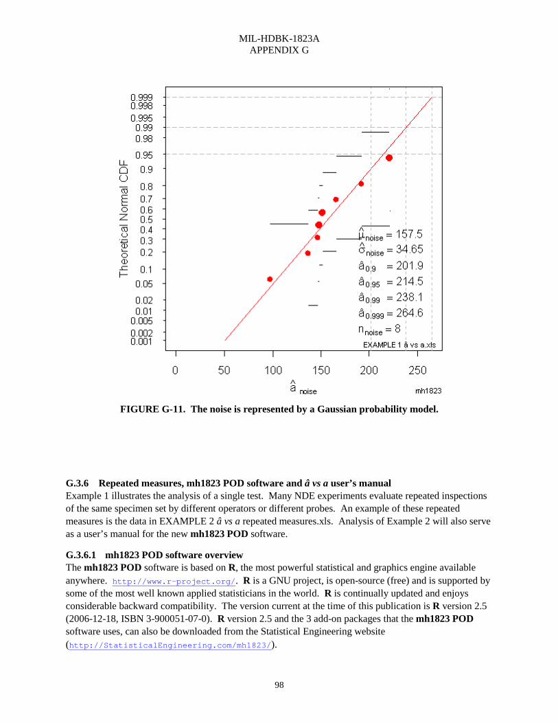
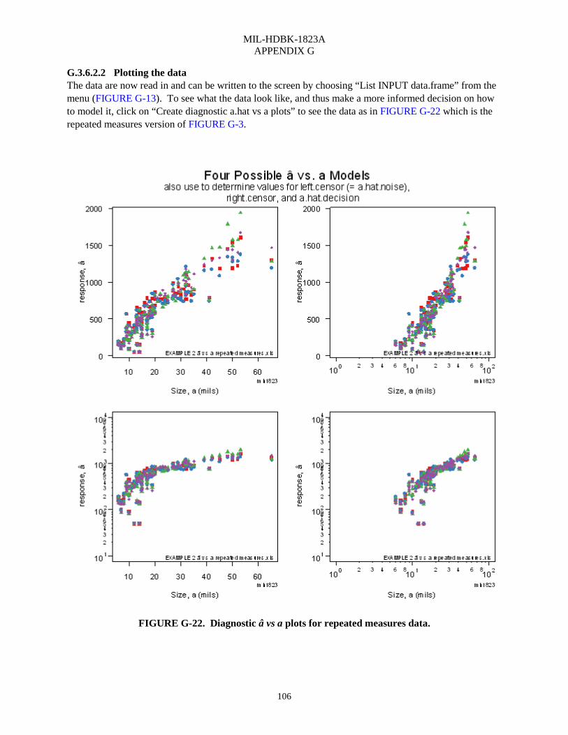
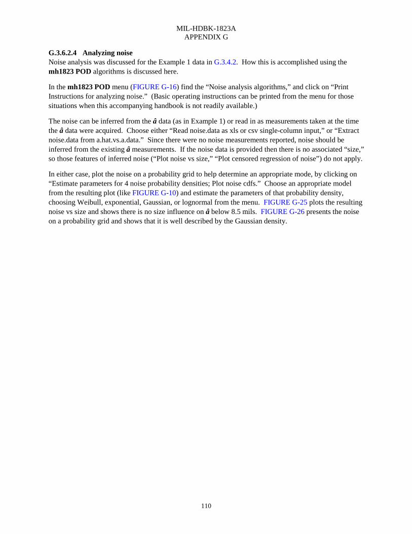
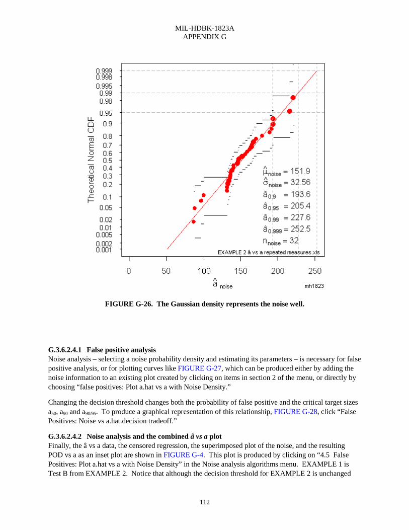
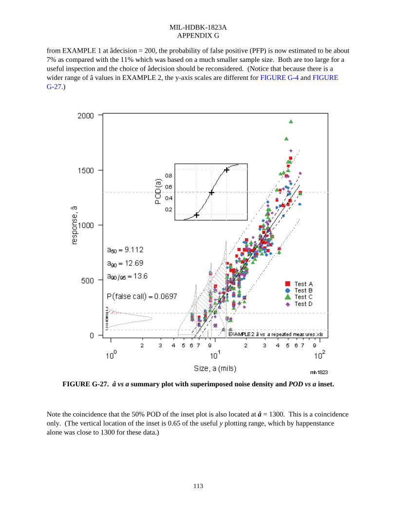
F.2.2.5 Target verification ............................................................................................................. 69 F.2.2.5.1 Specimen target response .................................................................................................. 70 F.2.2.5.2 Imbedded targets ............................................................................................................... 70 F.2.3 Specimen maintenance ..................................................................................................... 70 F.2.3.1 Handling............................................................................................................................ 70 F.2.3.2 Cleaning ............................................................................................................................ 70 F.2.3.2.1 Specimen integrity ............................................................................................................ 71 F.2.3.3 Shipping ............................................................................................................................ 71 F.2.3.4 Storage .............................................................................................................................. 71 F.2.3.5 Revalidation ...................................................................................................................... 71 F.2.3.6 Examples of NDE Specimens ........................................................................................... 72 Appendix G – Statistical Analysis of NDE Data ........................................................................................ 81 G.1 SCOPE .............................................................................................................................. 81 G.1.1 Scope ................................................................................................................................. 81 G.1.2 Limitations ........................................................................................................................ 81 G.1.3 Classification .................................................................................................................... 81 G.1.4 APPLICABLE DOCUMENTS ........................................................................................ 81 G.2 PROCEDURES ................................................................................................................ 81 G.2.1 Background ....................................................................................................................... 81 G.3 â vs a DATA ANALYSIS ................................................................................................ 85 G.3.1 Plot the data ...................................................................................................................... 85 G.3.2 Four guidelines ................................................................................................................. 86 G.3.3 Warning ............................................................................................................................ 86 G.3.4 How to analyze â vs a data ............................................................................................... 86 G.3.4.1 Wald method for building confidence bounds about a regression line ............................. 88 G.3.4.2 Understanding noise ......................................................................................................... 88 G.3.4.3 How to go from â vs a to POD vs a – The Delta Method ................................................. 89 G.3.4.4 The POD(a) curve ............................................................................................................. 92 G.3.5 How to analyze noise ........................................................................................................ 95 G.3.5.1 Definition of noise ............................................................................................................ 95 G.3.5.2 Noise measurements ......................................................................................................... 95 G.3.5.3 Choosing a probability density to describe the noise ........................................................ 96 G.3.6 Repeated measures, mh1823 POD software and â vs a user’s manual ............................. 98 G.3.6.1 mh1823 POD software overview ...................................................................................... 98 G.3.6.2 USER’S MANUAL ........................................................................................................ 100 G.3.6.2.1 Entering the data ............................................................................................................. 100 G.3.6.2.2 Plotting the data .............................................................................................................. 106 G.3.6.2.3 Beginning the analysis .................................................................................................... 108 G.3.6.2.4 Analyzing noise .............................................................................................................. 110 G.3.6.2.4.1 False positive analysis .................................................................................................... 112

MIL-HDBK-1823A


8

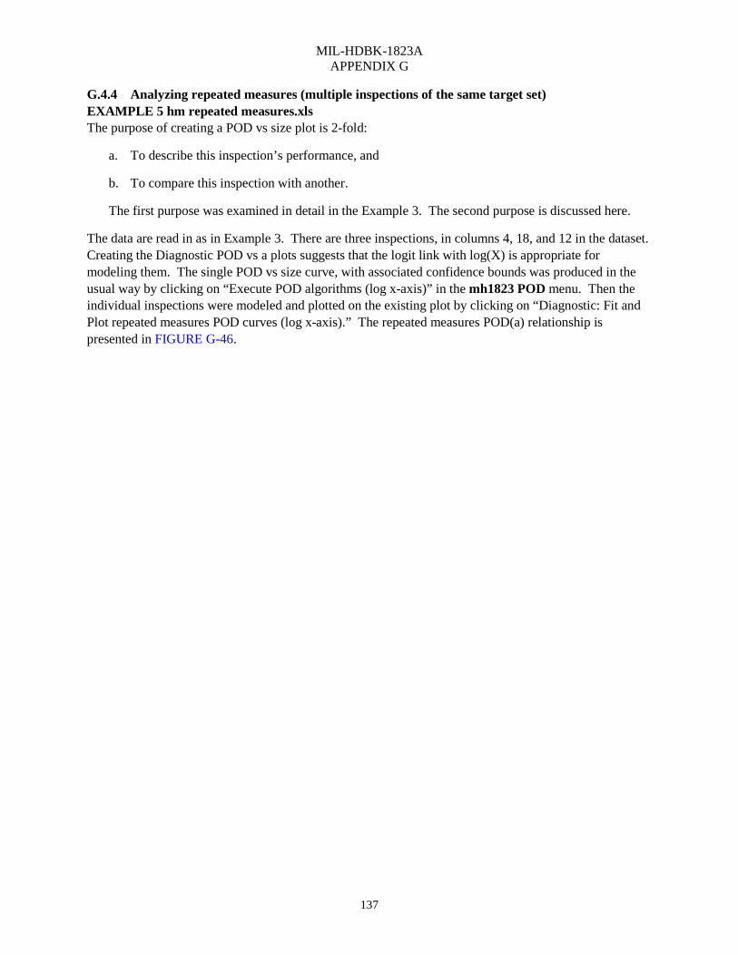
G.3.6.2.4.2 Noise analysis and the combined â vs a plot .................................................................. 112 G.3.6.2.5 The POD(a) curve ........................................................................................................... 114 G.3.6.2.6 Miscellaneous algorithms ............................................................................................... 119 G.4 Binary (hit/miss) data ...................................................................................................... 120 G.4.1 Generalized linear models............................................................................................... 120 G.4.1.1 Link functions ................................................................................................................. 120 G.4.2 USER’S MANUAL (Hit/Miss) ....................................................................................... 122 G.4.2.1 Reading in and analyzing hit/miss data – simple example (EXAMPLE 3 hm.xls) ........ 122 G.4.2.2 Constructing hit/miss confidence bounds ....................................................................... 130 G.4.2.2.1 How the loglikelihoood ratio criterion works ................................................................. 130 G.4.2.3 NTIAC data..................................................................................................................... 135 G.4.2.4 Lessons learned. .............................................................................................................. 135 G.4.3 Choosing an asymmetric link function: EXAMPLE 4 hm cloglog.xls ........................... 135 G.4.3.1 Analysis. ......................................................................................................................... 135 G.4.4 Analyzing repeated measures (multiple inspections of the same target set)

EXAMPLE 5 hm repeated measures.xls ........................................................................ 137 G.4.4.1 Analysis. ......................................................................................................................... 138 G.4.5 Analyzing disparate data correctly (EXAMPLE 6 hm DISPARATE disks.xls) ............ 139 G.4.5.1 Analysis .......................................................................................................................... 142 G.4.6 Analyzing hit/miss noise ................................................................................................. 142 G.5 mh1823 POD algorithms ................................................................................................ 144 Appendix H – Model-Assisted Determination of POD ............................................................................ 147 H.1 SCOPE ............................................................................................................................ 147 H.1.1 Scope ............................................................................................................................... 147 H.1.2 Limitations ...................................................................................................................... 147 H.1.3 Classification .................................................................................................................. 147 H.2 APPLICABLE DOCUMENTS ...................................................................................... 147 H.3 MAPOD .......................................................................................................................... 147 H.3.1 Protocol for model-assisted determination of POD ........................................................ 149 H.3.2 Protocol for determining influence of empirically assessed factors ............................... 149 H.3.2.1 Protocol for empirical â vs a model-building ................................................................. 152 H.3.2.2 Protocol for use of “physical” models to determine influence of model-assessed

factors.............................................................................................................................. 152 H.3.3 Summary ......................................................................................................................... 152 H.4 Examples of successful applications of MAPOD ........................................................... 152 H.4.1 Eddy Current detection of fatigue cracks in complex engine geometries ....................... 153 H.4.2 Ultrasonic capability to detect FBH’s in engine components made from a variety

of nickel-based superalloys ............................................................................................. 153 H.4.3 Capability of advanced eddy current technique to detect fatigue cracks in wing

lap joints .......................................................................................................................... 153

MIL-HDBK-1823A


9

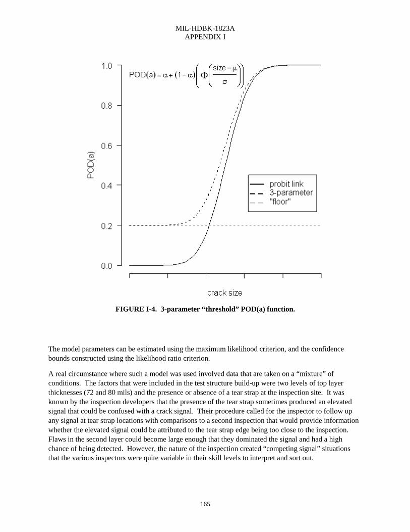
Appendix I – Special Topics ..................................................................................................................... 155 I.1 Departures from underlying assumptions – crack sizing and POD analysis of images .. 155 I.1.1 Uncertainty in X .............................................................................................................. 155 I.1.1.1 “Errors in variables” ....................................................................................................... 155 I.1.1.2 Summary – uncertainty in X ........................................................................................... 156 I.1.2 Uncertainty in Y .............................................................................................................. 156 I.1.2.1 Pre-processing – POD analysis of images ...................................................................... 156 I.1.2.1.1 How to go from UT image to POD ................................................................................. 157 I.1.2.1.2 Summary – POD analysis of images .............................................................................. 157 I.1.3 References ....................................................................................................................... 158 I.2 False positives, Sensitivity and Specificity ...................................................................... 158 I.2.1 Sensitivity, Specificity, positive predictive value, and negative predictive value ........... 158 I.2.2 Sensitivity and PPV are not the same .............................................................................. 158 I.2.3 Why Sensitivity and PPV are different ............................................................................ 159 I.2.4 Why bother to inspect? ................................................................................................... 159 I.2.5 Result to remember ......................................................................................................... 160 I.3 The misunderstood receiver operating characteristic (ROC) curve ................................ 160 I.3.1 The ROC curve ............................................................................................................... 160 I.3.2 Two deficiencies ............................................................................................................. 161 I.3.2.1 Prevalence matters .......................................................................................................... 161 I.3.2.2 ROC cannot consider target size ..................................................................................... 162 I.3.3 Summary ......................................................................................................................... 164 I.4 Asymptotic POD functions ............................................................................................. 164 I.4.1 A three-parameter POD(a) function ................................................................................ 164 I.5 A voluntary grading scheme for POD(a) studies ............................................................ 166 I.5.1 POD “grades” ................................................................................................................. 166 I.5.1.1 All POD studies .............................................................................................................. 166 I.5.1.2 Grade A ........................................................................................................................... 166 I.5.1.3 Grade B ........................................................................................................................... 167 I.5.1.4 Grade C ........................................................................................................................... 167 Appendix J – Related Documents ............................................................................................................. 169

MIL-HDBK-1823A


10

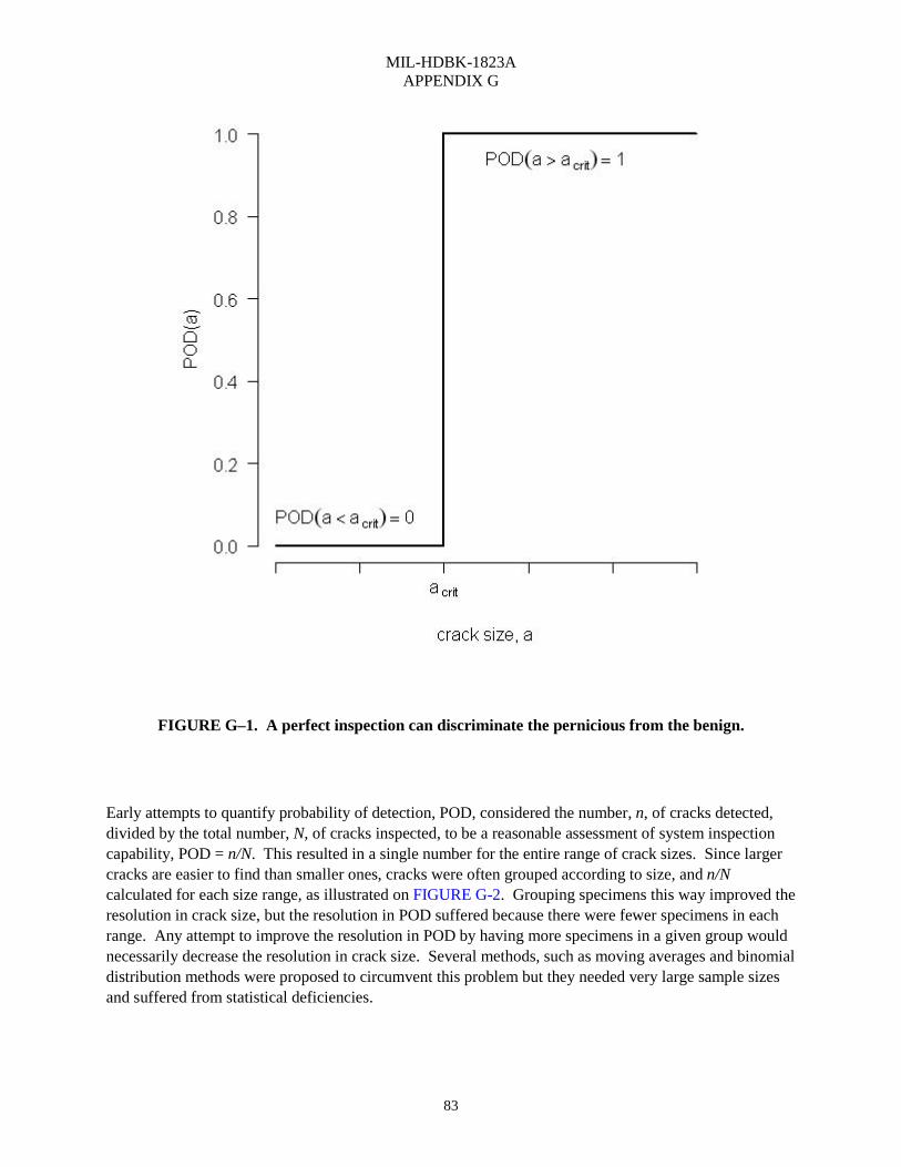
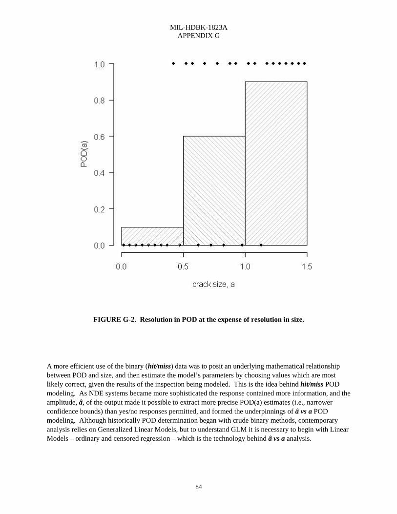
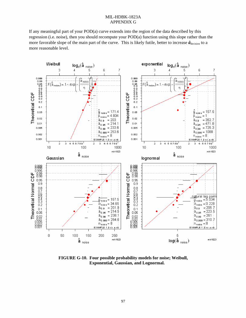
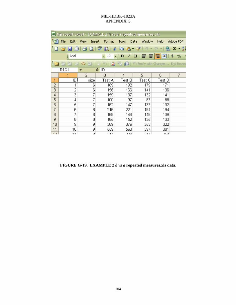
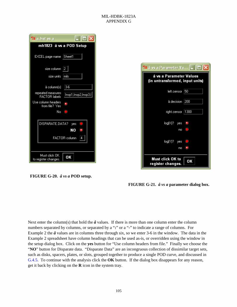
FIGURES FIGURE F-1. Typical FPI reliability demonstration specimen. ................................................................ 72 FIGURE F-2. Surface template for locating PT indications. ..................................................................... 73 FIGURE F-3. Typical engine disk circular scallop specimen. ................................................................... 74 FIGURE F-4. Typical engine disk elongated scallop specimen. ............................................................... 75 FIGURE F-5. Typical engine disk broach slot specimen. ......................................................................... 76 FIGURE F-6. UT internal target specimen. ............................................................................................... 77 FIGURE F-7. All targets on all rows are visible to interrogating sound paths. ......................................... 78 FIGURE F-8. “Wedding Cake” UT specimen. .......................................................................................... 79 FIGURE F-9. Typical engine disk bolt hole specimen. ............................................................................. 80 FIGURE G–1. A perfect inspection can discriminate the pernicious from the benign. ............................. 83 FIGURE G-2. Resolution in POD at the expense of resolution in size. .................................................... 84 FIGURE G-3. Diagnostic â vs a plots show log(X), Cartesian(Y) is the best model. ............................... 85 FIGURE G-4. â vs log(a) showing the relationship of â scatter, noise scatter, and POD. ........................ 87 FIGURE G-5. The Delta Method. .............................................................................................................. 90 FIGURE G-6. POD(a) curve for example 1 data (figure G-4) – log x-axis. .............................................. 92 FIGURE G-7. POD(a) curve for example 1 data (figure G-4) – Cartesian x-axis. .................................... 94 FIGURE G-8. Scatterplot of signal, â, vs size, a, showing only a random relationship. ........................... 95 FIGURE G-9. Regression model of noise â vs a showing an essentially zero slope. ................................ 96 FIGURE G-10. Four possible probability models for noise; Weibull, Exponential, Gaussian, and

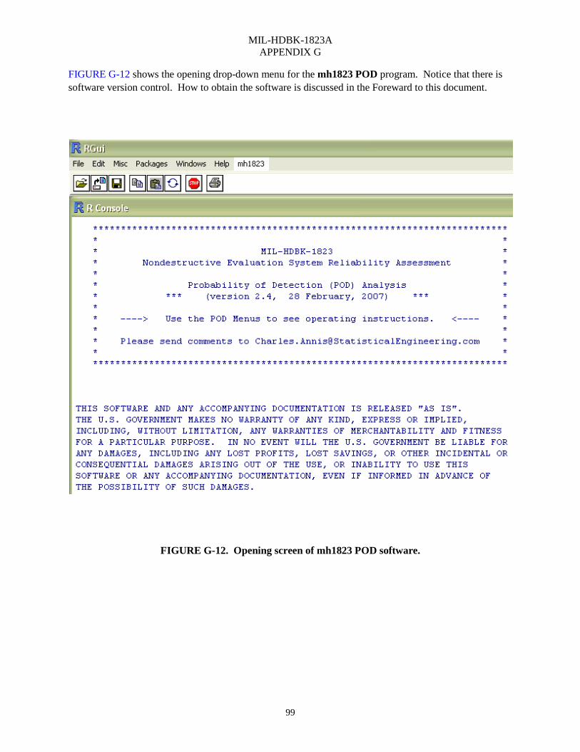
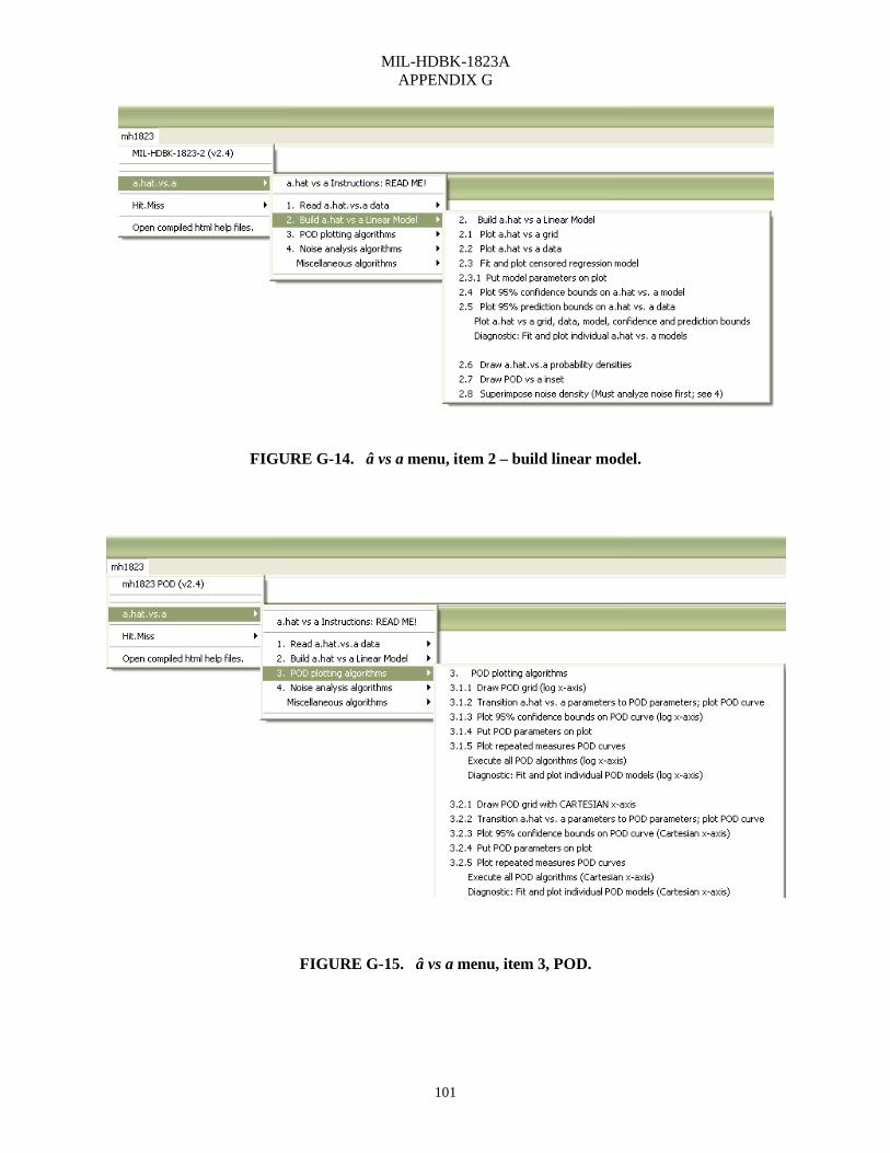
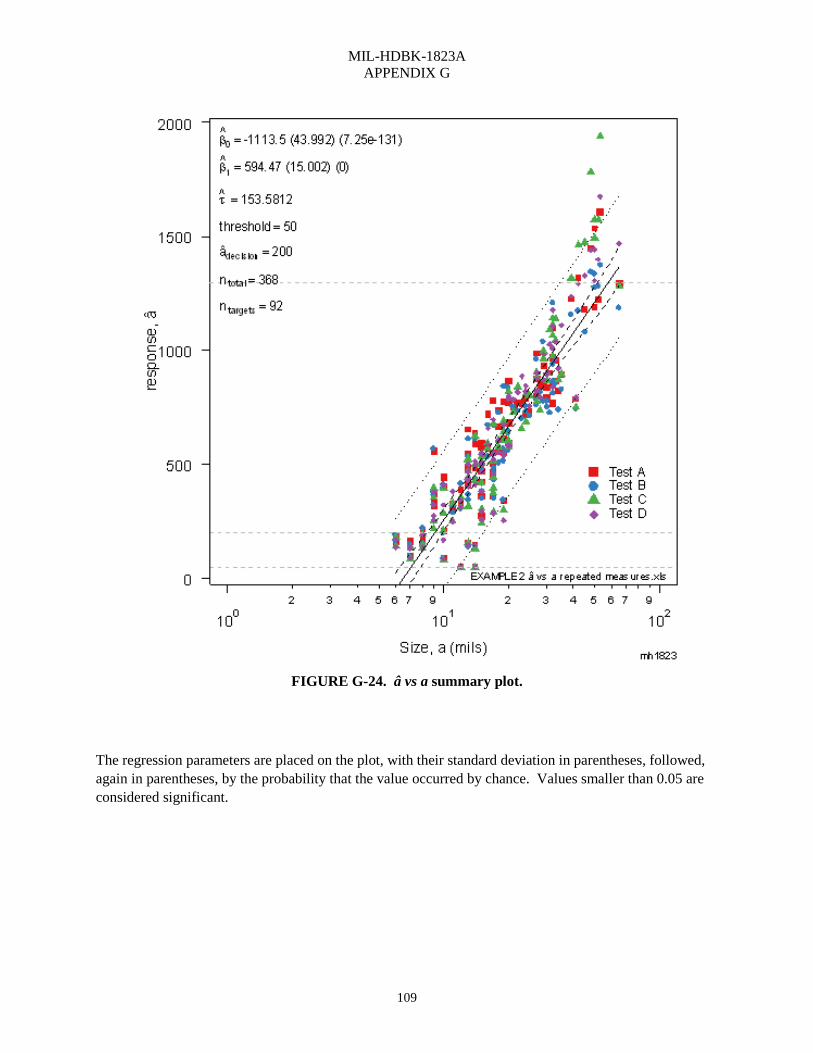
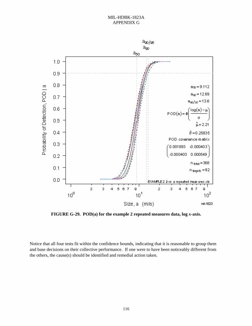
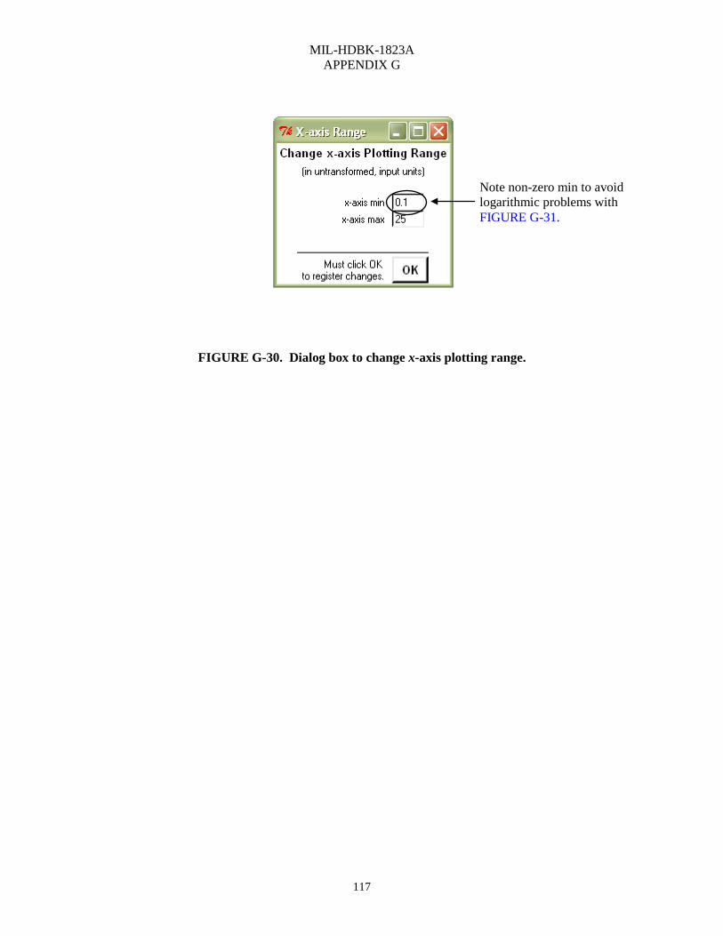
Lognormal. .................................................................................................................. 97 FIGURE G-11. The noise is represented by a Gaussian probability model. ............................................. 98 FIGURE G-12. Opening screen of mh1823 POD software. ...................................................................... 99 FIGURE G-13. â vs a menu, item 1 –– read â vs a data. ......................................................................... 100 FIGURE G-14. â vs a menu, item 2 – build linear model. ..................................................................... 101 FIGURE G-15. â vs a menu, item 3, POD. ............................................................................................. 101 FIGURE G-16. â vs a menu, item 4 – noise analysis. ............................................................................. 102 FIGURE G-17. â vs a menu, miscellaneous algorithms. ......................................................................... 102 FIGURE G-18. The â vs a dialog box. .................................................................................................... 103 FIGURE G-19. EXAMPLE 2 â vs a repeated measures.xls data. ........................................................... 104 FIGURE G-20. â vs a POD setup. ........................................................................................................... 105 FIGURE G-21. â vs a parameter dialog box. ........................................................................................... 105 FIGURE G-22. Diagnostic â vs a plots for repeated measures data. ....................................................... 106 FIGURE G-23. Example 2 data showing censoring values and âdecision. .................................................. 107 FIGURE G-24. â vs a summary plot........................................................................................................ 109 FIGURE G-25. Repeated measures noise. ............................................................................................... 111 FIGURE G-26. The Gaussian density represents the noise well. ............................................................ 112 FIGURE G-27. â vs a summary plot with superimposed noise density and POD vs a inset. .................. 113 FIGURE G-28. Trade-off plot showing PFP a90 and a90/5 as functions of âdecision. ................................... 114 FIGURE G-29. POD(a) for the example 2 repeated measures data, log x-axis. ...................................... 116 FIGURE G-30. Dialog box to change x-axis plotting range. ................................................................... 117

MIL-HDBK-1823A


11

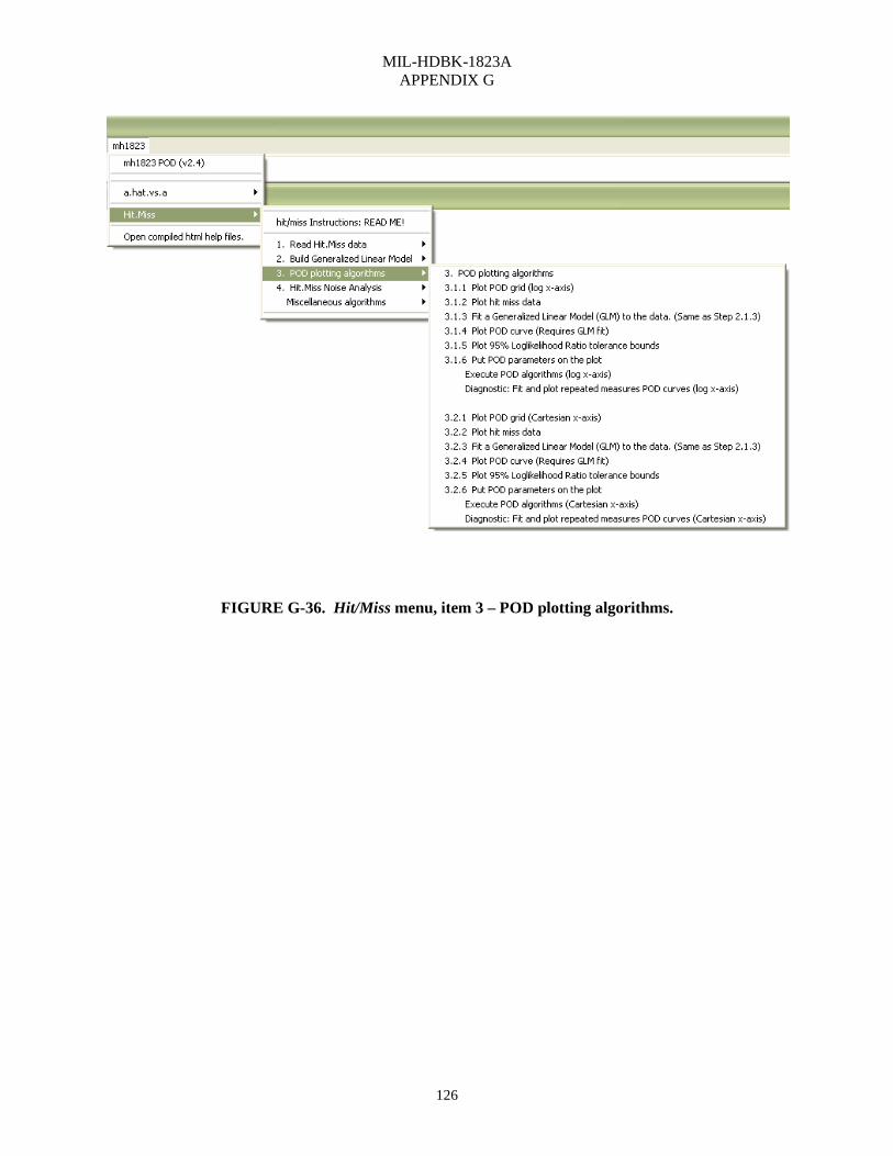
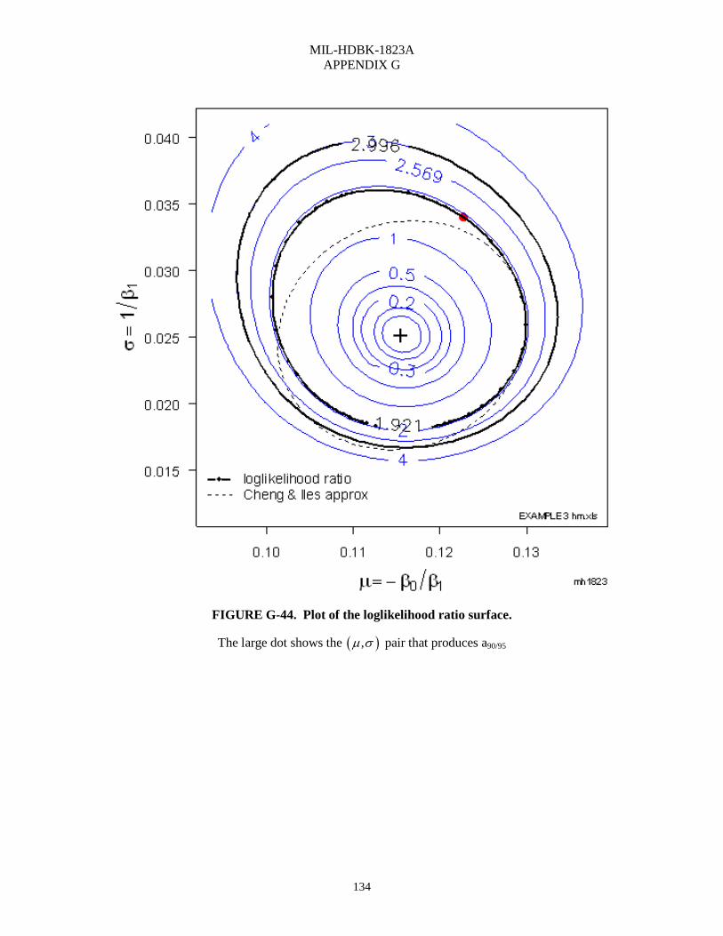
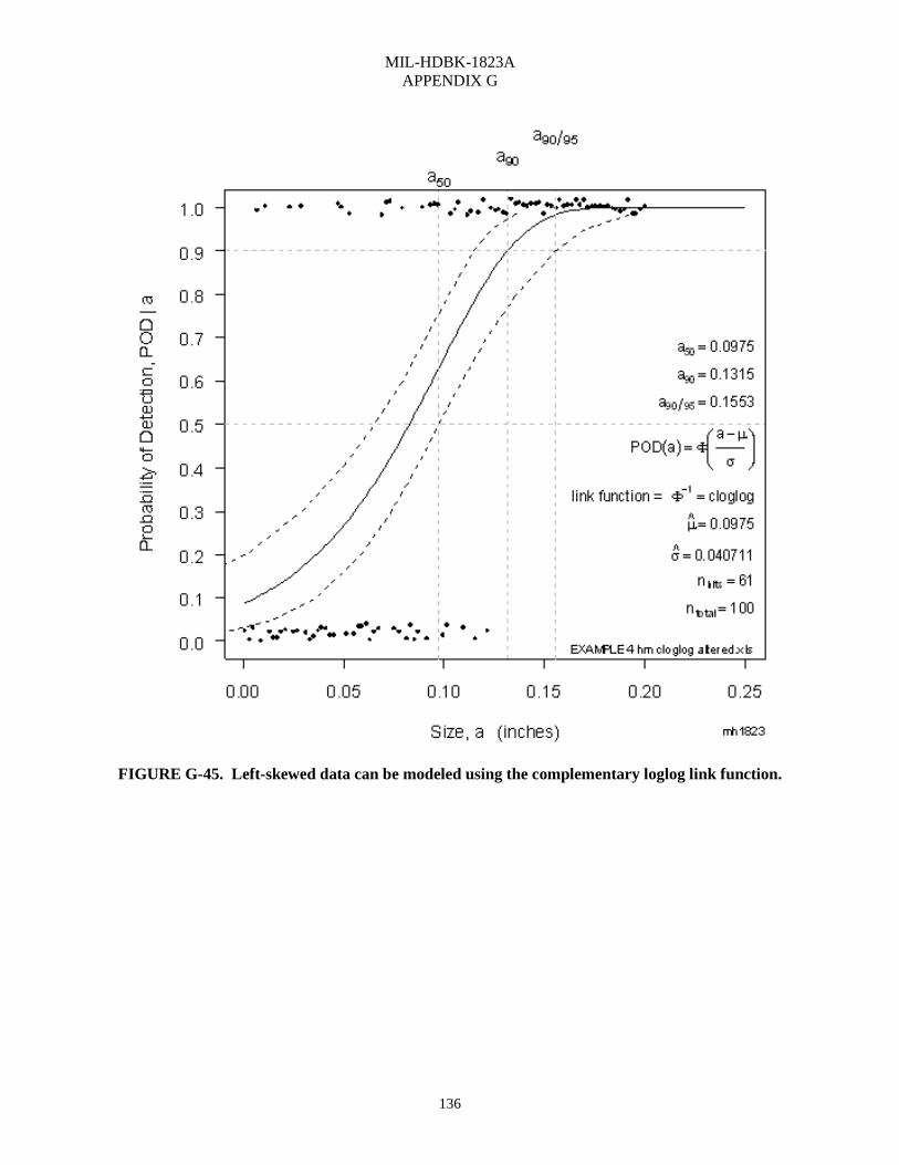
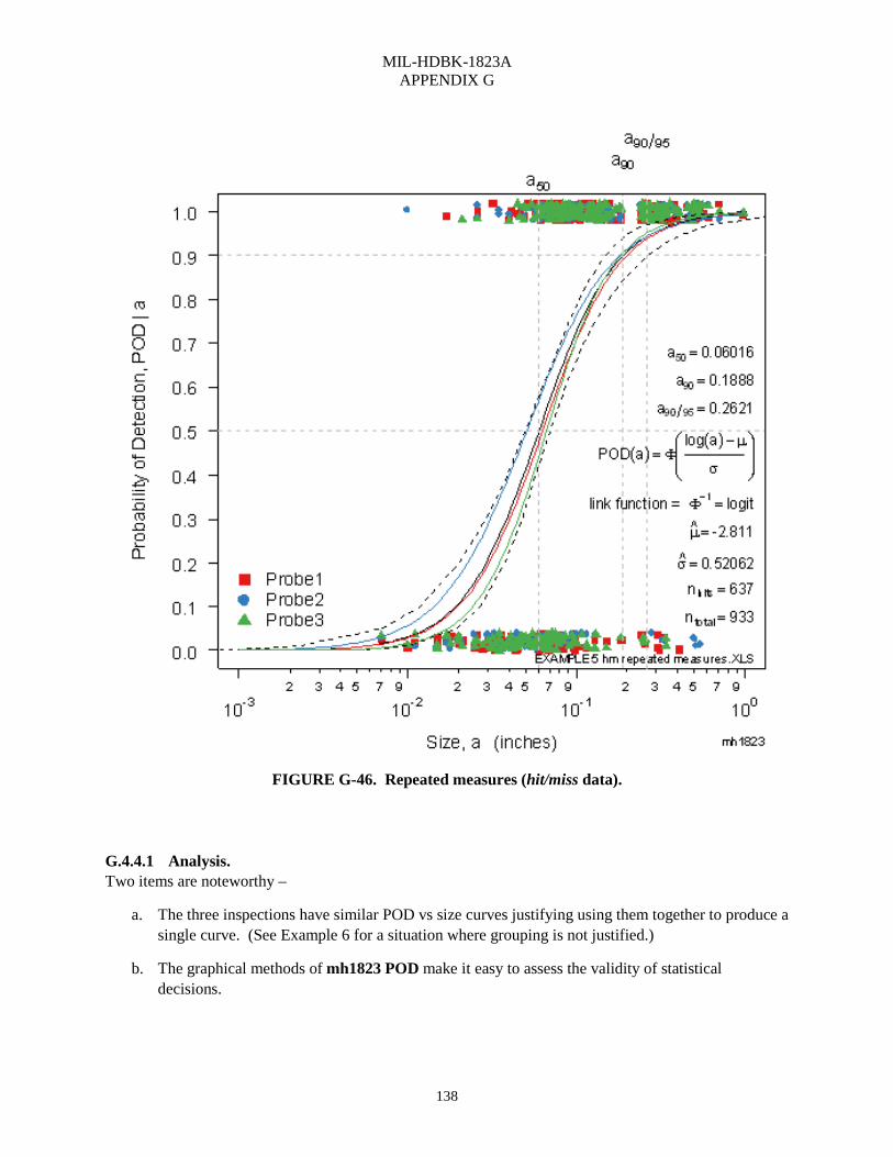
FIGURE G-31. POD(a) for the example 2 repeated measures data, Cartesian x-axis. ............................ 118 FIGURE G-32. POD vs size, EXAMPLE 3 hm.xls. ................................................................................ 123 FIGURE G-33. Hit/Miss menu, items 1 – read hit/miss data. .................................................................. 124 FIGURE G-34. Hit/Miss menu, item 2 – build generalized linear model. ............................................... 124 FIGURE G-35. Hit/Miss menu, item 4 – input hit/miss noise. ................................................................ 125 FIGURE G-36. Hit/Miss menu, item 3 – POD plotting algorithms. ........................................................ 126 FIGURE G-37. Hit/Miss menu – miscellaneous algorithms. ................................................................... 127 FIGURE G-38. Hit/Miss setup dialog box. .............................................................................................. 128 FIGURE G-39. Hit/Miss GLM parameter box. ....................................................................................... 128 FIGURE G-40. Choosing the right link function an whether to use log(size). ........................................ 129 FIGURE G-41. Plotting limits for the x-axis are adjustable. ................................................................... 130 FIGURE G-42. POD vs size model for EXAMPLE 3 hm.xls. ................................................................ 131 FIGURE G-43. POD vs size model for EXAMPLE 3 hm.xls, Cartesian POD y-axis. ........................... 132 FIGURE G-44. Plot of the loglikelihood ratio surface. ........................................................................... 134 FIGURE G-45. Left-skewed data can be modeled using the complementary loglog link function. ....... 136 FIGURE G-46. Repeated measures (hit/miss data).................................................................................. 138 FIGURE G-47. Disparate data (from 4 different disks) incorrectly grouped to produce an

“average” POD curve having a90/95 = 132 mils. ......................................................... 140 FIGURE G-48. Disparate data (from 4 different disks) showing the “average” POD curve does

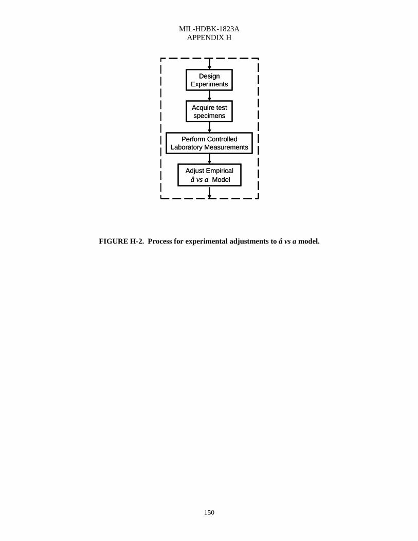
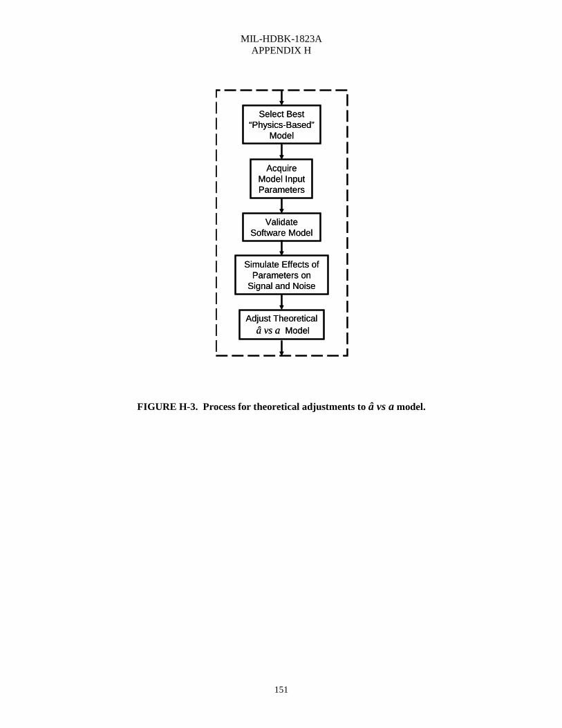
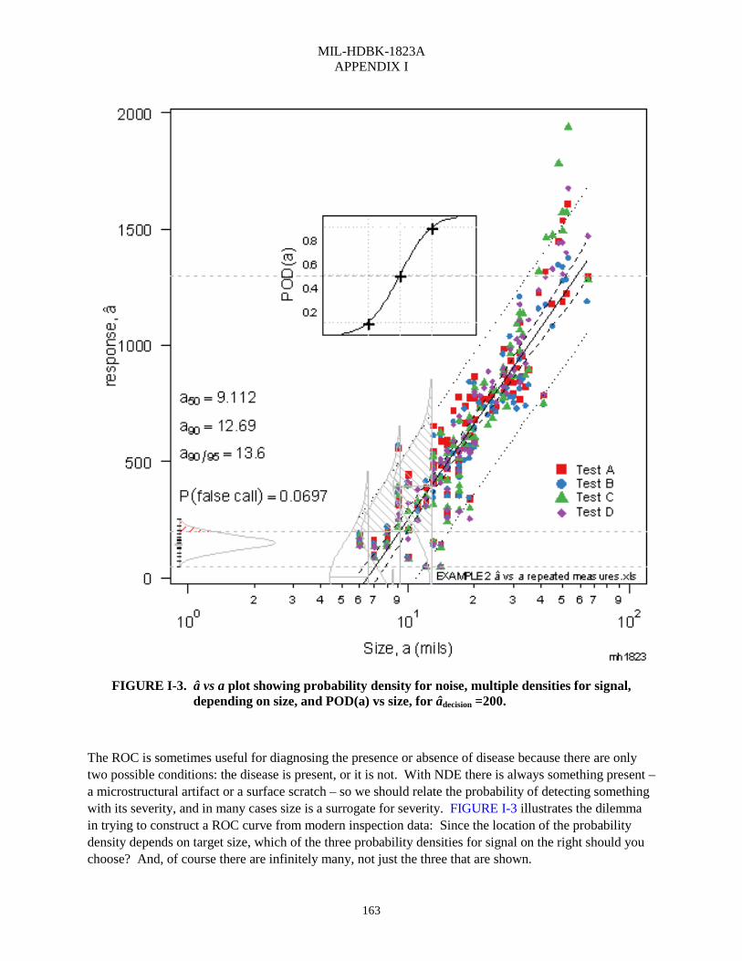
not represent any of them. ......................................................................................... 141 FIGURE G-49. Input data for Hit/Miss probability of false positive (PFP). ........................................... 143 FIGURE H–1. Model-assisted POD model building process. ................................................................. 148 FIGURE H-2. Process for experimental adjustments to â vs a model. .................................................... 150 FIGURE H-3. Process for theoretical adjustments to â vs a model. ........................................................ 151 FIGURE I-1. Receiver operating characteristic curve. ............................................................................ 161 FIGURE I-2. Noise and signal probability densities define the ROC curve............................................ 162 FIGURE I-3. â vs a plot showing probability density for noise, multiple densities for signal,

depending on size, and POD(a) vs size, for âdecision =200. ......................................... 163 FIGURE I-4. 3-parameter “threshold” POD(a) function. ........................................................................ 165 TABLES TABLE G-I. Results of PFP calculation with 1 hit in 150 opportunities. ................................................ 143 TABLE G-II. mh1823 POD algorithms. .................................................................................................. 144 TABLE I-I. Inspection and experiment have different objectives. .......................................................... 157 TABLE I-II. Generic contingency table of possible inspection outcomes. ............................................. 159 TABLE I-III. Contingency table of possible inspection outcomes – “good” inspection. ........................ 159 TABLE I-IV. Contingency table of possible inspection outcomes – coin-toss result. ............................ 160

MIL-HDBK-1823A

12

THIS PAGE INTENTIONALLY BLANK

MIL-HDBK-1823A

13

1. SCOPE

1.1 Scope This handbook applies to all agencies within the DoD and industry involving methods for testing and evaluation procedures for assessing Nondestructive Evaluation (NDE) system capability. This handbook is for guidance only. This handbook cannot be cited as a requirement. If it is, the contractor does not have to comply.

1.2 Limitations This handbook provides uniform guidance for establishing NDE procedures for inspecting flight propulsion system (gas turbine engines and rockets) components, airframe components, ground vehicle components, either new or in-service hardware, for which a measure of NDE reliability is needed. The methods include, but are not limited to, Eddy Current (EC), Fluorescent Penetrant (PT), Ultrasonic (UT), and Magnetic Particle (MT) testing. This document may be used for other NDE procedures, such as Radiographic testing, Holographic testing, and Shearographic testing, provided they produce an output similar to those listed herein and provide either a quantitative signal, â, or a binary response, hit/miss. Because the purpose is to relate Probability of Detection (POD) with target size (or any other meaningful feature like chemical composition), “size” (or feature characteristic) should be explicitly defined and be unambiguously measurable, i.e. other targets having similar measure will produce similar output from the NDE equipment. This is especially important for amorphous targets like corrosion damage or buried inclusions with a significant chemical reaction zone.

1.3 Classification NDE systems are classified into one of three categories:

a. those which produce only qualitative information as to the presence or absence of a flaw, i.e., hit/miss data,

b. systems which also provide some quantitative measure of the size of the target (e.g. flaw or crack) i.e., â vs a data,

c. systems which produce visual images of the target and its surroundings.

MIL-HDBK-1823A

14

2. APPLICABLE DOCUMENTS

2.1 General The documents listed below are not necessarily all of the documents referenced herein, but are those needed to understand the information provided by this handbook. See Appendix J for related documents of interest.

2.2 Government documents

2.2.1 Other Government documents, drawings, and publications The following other Government documents, drawings, and publications form a part of this document to the extent specified herein.

AFRL-ML-WP-TR-2001-4011 Probability of Detection (POD) Analysis for the Advanced Retirement for Cause (RFC)/Engine Structural Integrity Program (ENSIP) Nondestructive Evaluation (NDE) System Development Volume 2 – Users Manual (DTIC Accession Number ADA393072)

(Copies are available from Defense Technical Information Center (DTIC), 8725 John J. Kingman Road, Fort Belvoir VA 22060-6218 or online http://www.dtic.mil/dtic/.)

2.3 Non-Government publications The following documents form a part of this document to the extent specified herein.

THE R PROJECT FOR STATISTICAL COMPUTING

R – R is a free software environment for statistical computing and graphics

(The online source is http://www.r-project.org/.)

http://www.dtic.mil/dtic/�

http://www.r-project.org/�

MIL-HDBK-1823A

15

3. Nomenclature

a, size of discontinuity, flaw, or target

Physical dimension of a target – can be its depth, surface length, or diameter of a circular discontinuity, or radius of semi-circular or corner crack having the same cross-sectional area.

a , a-hat Measured response of the NDE system, to a target of size, a. Units depend on inspection apparatus, and can be scale divisions, counts, number of contiguous illuminated pixels, or millivolts.

50a Target size at 50% POD

ˆ deca , decision threshold Value of â above which the signal is interpreted as a hit, and below which the signal is interpreted as a miss. It is the a value associated with 50% POD. Decision threshold is always greater than or equal to inspection threshold.

ˆ sata , saturation Value of a as large, or larger than, the maximum output of the system or the largest value of a that the system can record.

ˆ tha , inspection threshold, signal threshold

Smallest value of a that the system records; the value of a below which the signal is indistinguishable from noise. Inspection threshold is always less than or equal to decision threshold.

0 1ˆ ˆβ β, Maximum likelihood estimators of parameters 0 1β β,

categorical variable Discrete variable having levels that are inappropriately described by simply assigning them a numerical code, and instead have a measurement scale based on categories.

calibration Process of determining the performance parameters of a system by comparing them with measurement standards.

Central Limit Theorem The distribution of an average tends to be normal, and regression model parameters tend to be asymptotically multivariate normal. Thus while the assumption of Gaussian behavior is not always appropriate for physical parameters, it is often justified for regression parameters.

censored data Signal response either smaller than ˆ tha , and therefore indistinguishable from the noise (left censored), or greater than ˆ sata (right censored), and therefore a saturated response.

Censored data require specialized statistical techniques because their likelihood function differs from uncensored observations at the same value.

coefficient Engineers and mathematicians say coefficient; statisticians say parameter, but these are not synonymous terms. A coefficient is a multiplier in a mathematical formula. A parameter is a numerical

MIL-HDBK-1823A

16

characteristic of a population or statistical model. µ σ, are parameters of the normal density. Their coefficients here are understood to be 1. The confusion arises in situations like this:

0 1y xβ β= + , where 0β and 1β are model parameters, but 1β is also the coefficient of x . Engineers and mathematicians see 0β and 1β as known, and x as unknown to be solved for, while statisticians view ( )x y, pairs as observed data and therefore known, from which the unknown 0β and 1β should be inferred.

components of variance In a designed experiment the total observed variance can be apportioned to its components (e.g.: probe, operator, underlying variance) so that improvements in inspection performance are possible, or the causes of substandard performance can be identified.

confidence The long run frequency of being correct. The maximum likelihood value for 90a is a best estimate for the target size with 90% POD, and so about half the time it is smaller than the true, but unknown, value and otherwise it is larger. A 95% confidence value for 90a (called 90/95a ) will be greater than the true 90a , in 95% of similar experiments.

conditional probability Probability of one variable, given the value of another, and given the model parameters: ( | , )f x y Θ where f is the probability of x by itself, given specific value of variable y, and the distribution parameters,Θ .

correlation A measure of the linear relationship between two variables. For example, when z x z− < < , the correlation between x and x2 is zero.

τ Sample standard deviation of residuals of regression of â against a referred to as standard error. An estimate of the standard deviation of the random error, ε.

Demonstration Design Document

The QA document that defines the plan for POD demonstration and data for maintaining and revalidating the suitability of POD test specimens.

detection Affirmative NDE system response, not necessarily rejectable.

deviance A measure of agreement between model and data. For linear models it is the sum of squares of the observations about their mean. For GLMs (hit/miss POD models) it is -2Lmax, where Lmax is the maximized loglikelihood.

disparate data Inspection data from difference specimen sets (usually from

MIL-HDBK-1823A

17

different equipment with different operators, probes, procedures) grouped to form one dataset, where the data are analyzed without explicit modeling or recognition of the differences. (See Appendix G, Example 6 hm)

DOE, DOX Design of Experiments – statistical methods for assigning test conditions to produce the maximum information with minimal expense.

ε Random error between assumed statistical model and measured system response.

ET Eddy current testing.

factor Variable whose effect on POD(a) is to be evaluated, especially a categorical variable, e.g. operator or probe.

false positive; false call NDE system response interpreted as having detected a target when none is present at the inspection location.

fitness for service Capability of a component or system to perform its intended function under given circumstances for a specified period of time.

GLM Generalized Linear Model – a regression having a binary (or otherwise non-continuous) response, such as hit/miss.

hit Affirmative NDE system response (detection) when flaw is present.

independent Two variables, A and B, are independent if their conditional probability is equal to their unconditional probability – A and B are independent if, and only if, ( | ) ( )P A B P A= , and

( | ) ( )P B A P B= . In engineering terms, A and B are independent if knowing something about one tells nothing about the other.

inference Process of drawing conclusions about a population based on measurements of samples from that population.

inspector Person administering the NDE technique who interprets the results and determines the acceptance of the material per specifications.

joint probability The probability of two or more things happening together, ( , | )f x y Θ where f is the probability of x and y together as a pair,

given the distribution parameters, Θ . A joint probability density of two or more variables is called a multivariate distribution.

likelihood The “probability of the data,” given specific model parameters, i.e., the probability that the experiment turned out the way it did as a function of model parameters.

MIL-HDBK-1823A

18

likelihood ratio method Method for constructing confidence bounds based on the asymptotic 2χ (chi-square) distribution of the loglikelihood. The likelihood ratio method produces confidence bounds on hit/miss POD(a) curves that are closer to their nominal values than does the Wald method.

linear model A regression.

marginal probability Probability of one variable for all possible values of another: ( | )f x Θ where f is the probability density of x, for all possible

values of y, given the distribution parameters, θ. The marginal probability of x is determined from the joint distribution of x and y by integrating over all values of y.

MAPOD Model-Assisted POD – methods for improving the effectiveness of POD models that need little or no further specimen testing.

maximum likelihood Standard statistical method used to estimate numerical values for model parameters such as 0 1β β, by choosing values that are most likely to have produced the observed outcome.

miss NDE system response interpreted as not having detected a target when one was present.

mixed models Statistical models for which the influence of a factor is described with a probability density rather than with individual parameter values.

MT Magnetic particle testing.

NDE/NDT Nondestructive evaluation/testing, which encompasses both the inspection itself and the subsequent statistical and engineering analyses of the inspection data.

NDE system Ensemble that can include hardware, software, materials, and procedures intended for the application of a specific NDE method. Can range from fully manually operated to fully automated.

NDI Nondestructive inspection. Often used interchangeably with NDE, however, should apply only to the inspection itself and not the subsequent data analysis.

noise Signal response containing no useful target characterization information.

ordinal variable Categorical variable that also has a hierarchal order. For example, “good,” “better,” “best,” are ordinal variables, and are based on an ordinal scale, where the distances between the ordered categories are unknown.

MIL-HDBK-1823A

19

parameter A numerical characteristic of a population or statistical model. µ σ, are parameters of the normal density.

PFP Probability of False Positive, or false call. PFP = 1 – specificity. =Prob(indication|no target present).

predictive value (positive) (PPV), P(defect | +): probability that the part has a defect, given a positive indication.

predictive value (negative) (NPV), P(no defect | -): probability that the part is defect-free, given a negative indication.

prevalence The fraction of defectives in a given population at a specific time.

POD , POD a| Probability of detection, given target a exists. POD = sensitivity.

( )POD a The fraction of targets of nominal size, a, expected to be found, given their existence.

probability 1) Frequentist definition – the long-run expected frequency of occurrence, P(event) = n/N, where n is the number of times event occurs in N opportunities. 2) Bayesian definition – a measure of the plausibility of an event given incomplete knowledge. Both definitions of probability follow the same mathematical rules.

PT Fluorescent penetrant testing.

QNDE Quantitative Nondestructive Evaluation.

quality assurance Any systematic process to see whether a product or service being developed is meeting specified requirements.

R Open-source (free) software environment for statistical computing and graphics. http://www.r-project.org/ ISBN 3-900051-07-0. The new mh1823 POD software uses as its computational and graphics engine.

regression Statistical model of the influence independent variables (e.g.: target size, probe type) on system output signal (â). Also called a “linear model.”

repeatability and reproducibility

Two potential components of variance. Repeatability often refers to equipment variation, with a single operator. Reproducibility often refers to the influence of different operators, using the same instrument to measure nominally identical characteristics. NOTE: these definitions are not universally agreed on and the usages of “reliability,” “repeatability,” “reproducibility,” “variability” and “capability” are often contradictory.


MIL-HDBK-1823A

20

residual Difference between an observed signal response and the response predicted from the statistical model. Residuals are only defined for non-censored observations.

sensitivity Probability of a true positive: P(detection | target present)

specificity Probability of a true negative: P(no indication | no target present)

“starburst”panel Panel or specimen containing a set of targets (artificial defects) that is used for periodic sensitivity tests of a PT system.

System Configuration Control Document

The QA document that defines the values of all system variables which will guarantee reproducible test results that can be related to integrity of the components under test.

system operator The person responsible for an automated or semi-automated system, including assuring that the mechanical, electrical, computer, and other systems are in proper operating condition.

target Object of an inspection. It can be a crack, flaw, defect, physical or chemical discontinuity, anomaly, or other origin of a positive NDE response.

UT Ultrasonic testing

Wald method Method for constructing confidence bounds on â vs a curves, and POD(a) curves derived from them, based on the asymptotic normal distribution of the model parameters. The Wald method is less often used in recent years for hit/miss POD in favor of the likelihood ratio method which produces confidence boundaries that come closer to achieving their nominal confidence levels. For â vs a data the difference between the Wald method and the likelihood ratio method are negligible.

MIL-HDBK-1823A

21

4. GENERAL GUIDANCE

4.1 General This section addresses the general guidance for assessing the capability of an NDE system in terms of the probability of detection (POD) as a function of target size, a. These general guidance are applicable to all NDE systems of this handbook and address responsibilities for planning, conducting, analyzing, and reporting NDE reliability evaluations. Specific guidance that pertain to eddy current test (ET), fluorescent penetrant test (PT), ultrasonic test (UT), and magnetic particle test (MT) inspection systems are contained in Appendix A through Appendix D.

4.2 System definition and control Before an NDT reliability demonstration is attempted, the contractor should conduct an evaluation of the complete NDE system in terms of the limits of operational parameters and range of application to demonstrate that the system is in control. At this time, the contractor can assess and list those factors that contribute most significantly to inspection variability as part of the System Configuration Control Document.

4.3 Calibration Calibration is the process of determining the performance parameters of a system by comparing them with measurement standards. A calibration ensures that the NDE system will produce results which meet some defined criteria with some specified degree of confidence, based on analysis of the system’s output and quantified by the POD(a) relationship. But the statistical POD analysis is only as good as the data on which it is based, and the data are only as good as the system that produced it, and that depends on effective calibration. (An excellent system, poorly calibrated, produces data of no consequence.) Because two points are needed to define a line, at least two different-sized references are needed to calibrate (or verify the calibration of) a system that produces a signal that is proportional to size, as NDE methods involving electronic measurements do. The calibration standards used for verification or recalibration should be substantially the same as to those that were used in the NDE demonstration, so that the POD(a) relationship that was demonstrated will apply to the recalibrated inspection.

4.4 Noise Since the recorded signal, â, is the aggregation of the target’s signature corrupted by aberrant signals collectively referred to as noise, the characteristics of the noise should be measured and reported along with the system response to known targets. Algorithms for determining a statistical model for the noise are provided in the companion software, mh1823 POD.

4.5 Demonstration design To ensure that the assessment of the NDE system is complete, documentation is developed which specifies the experimental design for the inspections; the method of obtaining and maintaining the structural specimens to be inspected; the procedures for performing the inspections; and the process for ensuring the inspection system is under control. The topics that are to be addressed in each of these areas include the following.

4.5.1 Experimental design The objective of an NDE reliability demonstration is not to determine the smallest crack the system can find – it is to determine the largest crack the system can miss. To do this we should establish the relationship between POD and target size (or other variables) that defines the capability of an NDE

MIL-HDBK-1823A

22

system under representative application conditions. In addition we should determine the potential for false positives (false calls) at each set of conditions, because a POD estimate has little utility if it is accompanied by an unacceptable false positive rate. Variation in NDE system response (and, hence, uncertainty in target detection) is caused by both the physical attributes of the targets under test, and the NDE process variables, system settings, and test protocol. The uncertainty caused by differences between targets is accounted for by using representative specimens with targets of known size (and other characteristics to be evaluated) in the demonstration inspections (see 4.5.2). The uncertainty caused by the NDE process is accounted for by a test matrix of different inspections to be performed on the complete set of specimens.

a. The experimental design defines the conditions related to the NDE process parameters under which the demonstration inspections will be performed. In particular, the experimental design comprises:

(1) The identification of the process variables which may influence target detection but cannot be precisely controlled in the real inspection environment;

(2) The specification of a matrix of inspection conditions which fairly represents the real inspection environment by accounting for the influencing variables in a manner which permits valid analyses;

(3) The order for performing the individual inspections of the test matrix. The number of flawed and unflawed inspection sites in the experiment could also be considered as part of the experimental design.

b. Although general guidelines for these areas are presented in the following paragraphs, and the necessary statistical analysis software (mh1823 POD) is freely available, it is recommended that a qualified statistician participate in the preparation of the experimental design and in the subsequent analyses. Be aware that poor attention to significant test variables will produce erroneous or misleading results. Furthermore, the inspection process can be sufficiently complex that it is difficult to determine whether or not an accurate performance estimate has been obtained. Poor planning cannot be remedied after the data are collected.

4.5.1.1 Test variables The inspection process should be defined by the responsible engineer and under control before the capability demonstration is initiated, as indicated in 4.2. Every controlled NDT system contains variables that should be defined and tested during the demonstration. To evaluate the inspection system in the application environment, these variables should be identified so that they can be fairly represented in the demonstration tests. If poor attention is paid to identification and tracking of significant test variables, then the NDT demonstration is invalid. For example, in a manual inspection, it is unacceptable to use only the known best inspector in the demonstration tests. Rather, the entire population of inspectors should be represented.

a. The contractor generates a list of process variables which can be expected to influence the efficacy of the NDE system. This list provides the basis for generating the evaluation test matrix. To assure a thorough evaluation, the initial matrix should include as many variables as possible. If early in the test program it is demonstrated that a variable is not significant, it may be eliminated from further consideration, resulting in a revised, smaller test matrix. To be

MIL-HDBK-1823A

23

eliminated, it should be shown that the variable has no significant effect on POD using the analysis methods as specified in Appendix G. The Government reserves the right to expand or reduce the list of variables to be included in the test matrix. The list of significant variables will be strongly controlled by the type of NDT process and its specific application.

b. As a minimum, the following types of variables should be considered in generating the list of test variables:

(1) Specimen pre-processing: This variable includes factors such as typical in-service contamination, chemical cleaning, abrasive blast, access to tight radius regions, and general surface condition. It could also include such things as the application of the penetrant for fluorescent penetrant readers. Early in the definition of the system acceptance test plan, a decision is made as to how far upstream the variables should extend. For a penetrant reading system, it might be decided not to consider the penetrant application as a variable and thus to hold that constant for all systems being compared. If, however, a complete PT system is being evaluated, all process variables should be included in the test plan. The ranges of the variables to be considered are those allowed by the procedures used at the application site.

(2) Inspector: In many applications the human conducting the inspection is the most significant variable in the process. Some inspection systems have been demonstrated to be very inspector-independent. The test plan should include several operators selected at random from among the population eligible to conduct the inspections. Eligibility is defined in terms of certification, training, or physical ability.

(3) Inspection materials: These are particular chemicals, concentrations, particle sizes, and other material-dependent variables to be used in a given inspection. For example, PT inspections use penetrants, emulsifiers and developers, each of which may have a significant influence on inspection capability. System evaluation is conducted considering the range of materials expected to be used in production. If for example different penetrants are used, the penetrant should be considered as a variable in defining the test matrix. If the operating procedures for the system preclude the use of alternate penetrants, others need not be included, but this restriction clearly limits the generality of the system assessment.

(4) Sensor: If the sensor used in the inspection system is replaceable, or if different sensors are used for different applications of the system such as is the case for eddy current or ultrasonic inspections, sensors are necessarily a variable in the test matrix. The sensors used in the demonstration tests should be selected at random from a production lot. Sensor designs typical of each planned for use with the system should be included in the test plan, with several of each being evaluated.

(5) Inspection setup (Calibration): Electronic inspection processes in particular need instrumentation adjustments to assure the same sensitivity inspection independent of time or place. To evaluate the potential variation introduced to the inspection process by this calibration operation, the test matrix should include calibration repetitions, allowing random variations that are consistent with the process instructions. If more than one calibration standard is available (e.g. production sets), the effect of the variation among standards should also be considered as a test variable by repeating the specimen inspection after calibrating on each of the available standards.

MIL-HDBK-1823A

24

(6) Inspection process: The inspection process specifies controls on inspection parameters like dwell time, current direction, scan rates, and scan path index. The system test matrix should include evaluation of these parameters. If an allowable range is specified, the test plan should evaluate the inspection at the extremes of this range. If the parameter is automatically to be held constant, repetitions of the basic inspection may be sufficient evaluation of this variable.

(7) Imaging considerations: If the inspection process produces an image for inspection personnel to assess and make pass/fail decisions, then all significant variables associated with the imaging process itself should be considered. These variables should be defined by the responsible engineer and may include initial image processing in hardware or software, image size, brightness, contrast, color enhancement, ambient lighting, special focusing techniques and area of consideration. Since the mh1823 POD software is used to produce a POD vs size plot, “size” should be explicitly defined. This is especially important for amorphous targets like corrosion damage or buried inclusions with a significant chemical reaction zone. (See I.1.2.1)

4.5.1.2 Test matrix The contractor should generate a test matrix to be used in the reliability demonstration. The test matrix is a list of planned process test conditions which collectively define one or more experiments for assessing NDE system capability. A process test condition is defined as a set of specific values for each of the process variables deemed significant. The complete set of test specimens is inspected at each test condition in the test matrix. The complete matrix can comprise more than one experiment to allow for preliminary evaluation of variables which may only slightly influence inspection response of the system. To the extent possible, the individual inspections of a single experiment should be performed in a random order to minimize the effects of all uncontrolled factors which might influence the inspection results.

a. The inspection test conditions should be representative of those that will be present at the time of typical inspections. The values assigned to each test variable should be assigned at random to minimize unexpected, hidden influences. For example, if a future inspection is to be performed by any of a given population of inspectors and three inspectors are to be included in the experiment, then the three inspectors should be chosen at random. Similarly, if two different probes of identical design are to be used in the experiment, they should be selected at random from the population of probes. Note that if the population of probes (or inspectors) includes those not yet available, it is assumed that the available probes (or inspectors) are representative of those that will be used in the future.

b. In the past, factorial experiments, which test all combinations of given levels for the variables, or fractional factorial designs, were suggested for NDE experiments. Factorial designs, however, are screening designs for evaluating a large number of variables for the purpose of eliminating most of them. Response surface designs, which do share some fractional factorial characteristics, are better suited for NDE demonstration experiments because they measure the influence and variability of important variables, rather than identify unimportant ones, although that is sometimes the goal of exploratory experiments on altogether new systems.

c. Like much in engineering, the final test matrix will be a compromise among the number of variables that can be included, the number of levels (values) for them, and the available time and money.

MIL-HDBK-1823A

25

d. Experiments to evaluate the effects of inspection process parameters on POD can be designed and analyzed using the methods of Appendix E, especially E.3.2.7, and Appendix G. Such experiments should be performed as part of the capability demonstration as a planned approach to optimizing the process.

4.5.2 Test specimens The test specimens should reflect the structural types that the NDE process will encounter in application with respect to geometry, material, part processing, surface condition, and, to the extent possible, target characteristics.

a. Since a single NDE process may be used on several structural types, multiple specimen sets may be needed in a reliability assessment. The contractor should determine the characteristics of the test specimens and recommend the number of flawed and unflawed specimens. All test specimens available to the contractor should be evaluated to determine if existing test sets meet the guidance of the reliability demonstration.

b. It is critical to assess the types of targets that are provided by the specimens to assure that they are valid for the upcoming demonstration. For example, if the targets are fatigue cracks they should be generated in a manner that represents field conditions, otherwise, the demonstration may be unnecessarily difficult or uselessly easy. In some cases it may be possible to compare defect signatures between specimens and rejected hardware to demonstrate similitude.

c. The contractor should insure that the specimens do not become familiar to the inspectors or inspection system. Such familiarity does not represent typical inspections and any such demonstration is thereby tainted.

(1) In some cases, it may be appropriate to allow inspectors and their supervision to use a small subset, or “training set,” of specimens to prepare the NDT system for the demonstration.

(2) In other situations new specimen sets may be needed to meet the guidance.

d. A plan for maintaining and re-validating the specimens is to be established and all results documented in the Demonstration Design Document. The following paragraphs present minimum considerations in obtaining and maintaining the demonstration test sets. Further guidelines for fabricating, documenting, and maintaining test specimens are presented in Appendix F.

4.5.2.1 Physical characteristics of the test specimens Specimens should closely resemble the subject parts that are being tested by the demonstrated NDE system.

a. Specimens should closely mimic the local geometries of the actual hardware for inspections where probe manipulation or significant features of the inspection process (such as magnetic field, sound waves, and line of sight) are geometry dependent. Bolt holes (FIGURE F-9), flat surfaces, fillets, radii, slots (FIGURE F-5), and scallops (FIGURE F-3 and FIGURE F-4) are some typical shapes that influence inspections.

b. Residual stress which has resulted from raw material processes, manufacturing processes, part geometry and service history may produce major influences on the inspection. This has been

MIL-HDBK-1823A

26

documented with PT, ET and UT. Residual stresses can also be influenced by final machining and by crack propagation, as cracks can grow to relieve the stress field in which they reside.

c. Flaw location and orientation are significant geometric considerations for most inspection techniques (for example, corner flaws versus surface cracks.) Flaw locations in specimens should be oriented and positioned to represent cracks that have been recorded in actual parts. In the case where NDE or failure analysis has provided this critical information, use the best available structural design information. The initial geometry of the specimen should allow the insertion of targets of the shape and size in the specified locations. The specimen should be designed such that the targets can be inserted, and the final geometry obtained by machining or other forming methods that will not change the target characteristics (size, shape, and orientation and intended location). Reasonable distance depends on the inspection that is being demonstrated. For example, flaw location accuracy is less critical for PT (often ±0.010 inch) than it is for automated ET (often ±0.002 inch.) Specimens should be manufactured to tolerances typical of the component they represent. The specimen designer should be aware that manufacturing costs rise as critical dimensions are tightened.

d. For most NDE methods the contractor should select alloys, material forms, and raw material processing that represent the significant physical properties for the method being evaluated. For example, if an actual part is made of INCO 718, forged to near finished shape, a UT specimen should be made of INCO 718 and fabricated by the same processes. In addition, for UT, the internal noise and attenuation should be as defined by the QA documents supplied by the OEM for the components to be inspected. For magnetic particle inspection, the magnetic properties should be comparable to the components to be inspected. Grain size can have a large influence on signal to noise ratio for ET and UT. Material strength can influence the amount of smear metal which can obscure defects from penetrant inspection.

e. Surface condition of the specimen may influence inspection signal-to-noise ratios. Final machining of the specimen should be consistent with final machining of the part. The surface finish of the specimen and actual part should be consistent so that the common surface finish between specimen and part provide similar signal responses. For example, if the part is turned on a lathe, the specimen should be turned on a lathe whenever possible. If the surface texture of the part and specimen are not similar, for instance “record groove” finish on the part due to lathe turning and ground finish on the specimen from grinding, the false positive rate may be higher on the parts due to the macro finish of record groove even though the micro surface finishes are similar.

f. PT is one process where it is possible to make some careful material substitutions. For example, it is common for a less-expensive forged Inconel product to be used for PT specimens that are involved in testing inspections of powder metallurgy engine disks. In this case, surface condition and residual stress are bigger influences than basic material chemistry.

4.5.2.2 Target sizes and number of “flawed” and “unflawed” inspection sites The statistical precision of the estimated POD(a) function depends on the number of inspection sites with targets, the size of the targets at the inspection sites, and the basic nature of the inspection result (hit/miss or magnitude of signal response). Unflawed inspection sites are necessary in the specimen set to preclude guessing and to estimate the rate of false indications.

MIL-HDBK-1823A

27

a. In the 1980s consensus was that target sizes should be uniformly distributed on a log scale covering the expected range of increase of the POD(a) function. This results in fewer large targets and more small ones. Recent work1 indicates that more precise estimates of a90 and narrower confidence bounds on the POD(a) curve result from target sizes that are uniformly spaced on a Cartesian scale and therefore this is the new recommended practice.

(1) Given that a90/95 has become a de facto design criterion it may be more important to estimate the 90th percentile more precisely than lower parts of the curve. This can be accomplished by placing more targets in the region of the a90 value but with a range of sizes so the entire curve can still be estimated. One way to accomplish this is to space them uniformly on a Cartesian scale rather than on the log scale.

(2) Since it can be difficult to produce small targets precisely (the actual sizes are often much larger than desired) great care should be exercised to ensure that the desired smaller targets have been achieved. Cracks which are so large that they are always found (or saturate the recording device) or so small that they are always missed (or produce a signal which is obscured by the system noise) provide only limited information about the POD(a) function.

(3) If it is possible to estimate in advance the specific region where the POD(a) function rises rapidly, then it is advantageous to concentrate more targets in that size range. It should be noted that there is a tendency to include too many “large” targets in NDE reliability demonstrations, as a result of the difficulties in producing small targets in specimens.

b. To provide reasonable precision in the estimates of the POD(a) function, experience suggests that the specimen test set contain at least 60 targeted sites if the system provides only a binary, hit/miss response and at least 40 targeted sites if the system provides a quantitative target response, â. These numbers are minimums. For binary responses, 120 inspection opportunities will result in a significantly more precise estimate of a50, and thus a smaller value for a90/95.

c. To allow for an estimate of the false positive rate, the specimen set should contain at least three times as many unflawed inspection sites as flawed sites. An unflawed inspection site need not be a separate specimen. If a specimen presents several locations which might contain targets, each location may be considered an inspection site. To be considered as such, the sites should be independent, that is, knowledge of the presence or absence of a target at a particular site cannot influence the inspection outcome at another site. It is advisable to have at least 10 to 20 unflawed specimens for PT testing.

4.5.2.3 Specimen maintenance The contractor should devise a plan for protecting the specimens from mechanical damage and contamination that would alter the response of the NDE process for which they are used. Many specimen sets have been ruined due to mishandling during demonstrations and clean-up. As a minimum the specimens should be:

a. Individually packaged in protective enclosures when not in use;

b. Carefully handled when in use;

1 Private communications between Charles Annis, P.E., Alan Berens, Ph.D. and Floyd Spencer, Ph.D.

MIL-HDBK-1823A

28

c. Cleaned immediately and returned to the protective enclosure after each use;

d. Re-validated at intervals specified by the contracting agency when the specimens are intended for periodic usage.

4.5.2.4 Specimen flaw response measurement Specimen flaw responses are to be measured periodically by the contractor, as monitored by the appropriate procuring activity using the same test technique and procedure used in the original specimen verification (Appendix F). The target response should fall within the range of the responses measured in the original verification process. If it does not, the results should be examined to consider if they are acceptable, if the specimen has been unacceptably compromised, or if the specimen needs to be re-characterized and verified.

4.5.2.5 Multiple specimen sets When multiple specimen sets are needed for periodic use, the contractor should select one set as a master set. The remaining sets are to be demonstrated to have a response within a specified tolerance of the master set. A plan for periodic re-verification against the master set should be documented and the re-verification carried out as mandated by the contract.

4.5.2.6 Use of actual hardware as specimens In many cases when an NDE development system is first being evaluated, the specific part geometries and surface conditions may not be known, or if known, representative flawed specimens may not be available, whereas similar hardware may be. These may not represent exactly the conditions in the specific application of the system, but will be more realistic than laboratory specimens alone. The parts can have targets/defects in them to provide signals for the inspection, or known to be unflawed and thus used to provide noise measurements. For ET and MT systems, EDM notches may be sufficient for evaluating scan plan coverage but are insufficient to assess system response to actual fatigue flaws. The use of MAPOD (Model-Assisted POD, discussed in Appendix H) can help account for differences in crack/slot responses. For UT, drilled holes may be preferable; for PT, fluorescent markings may be the best available, though they may be too bright to verify system capabilities. An ideal test would use actual service flawed hardware, if a representative selection of such parts were available, and the characteristics of the flaw, crack, or defect can be measured.

4.5.3 Test procedures The contractor should develop and report a detailed plan for executing the demonstration tests at the application facility. The procedures to be used in the demonstration should follow the procedures and work instructions planned for the production inspection of parts. The test procedure that most closely resembles the work instruction or nondestructive test method may be the best demonstration procedure. This includes all fixed process parameters, data analysis algorithms (for automated systems), accept/reject criteria and other items covered by the System Configuration Control Document. The inspections are to be performed by production inspectors, as designated by the experimental design. A test monitor is to be designated to assure that all guidance of this handbook are met both in the planning and during the performance of the tests, and who is accountable.

a. Every inspection technology depends on certain conditions being met that the operator may not be able to verify as a part of the daily inspection setup. Examples include the scan speed or index of mechanical manipulators, the drive frequencies of eddy current or ultrasonic instruments, or

MIL-HDBK-1823A

29

the purity of chemicals or solutions being used. Prior to the NDE system evaluation these significant variables should be calibrated. This can be done using NIST-traceable standards and procedures. Note that any nonconformance not corrected will render the results suspect. Periodic recalibration of the NDE system after acceptance should be conducted in accordance with local procedures.

b. In addition to specific guidance of the NDE process (see 5, and Appendix A, Appendix B, Appendix C, or Appendix D), the following should be considered in the development of the test procedure plan:

(1) System software controlling any data collection, reduction, and processing should be that planned for use in production implementation. Any differences between the test and in-service inspection could render the POD curve unfit for its intended usage.

(2) Appropriate fixturing of specimens can make the inspection procedure similar to actual parts; that is, the demonstration fixturing and the actual component would ideally have the same inspection system arrangement of probe, orientation, manipulation, and scan plan.

(3) Signal evaluation and decision levels used during the testing should be those planned for use in production. In many cases it may not be known in advance what thresholds can be practically implemented in production. In these situations the detection capabilities should be established as a function of these process parameters. The accompanying mh1823 POD software provides for threshold POD trade-offs.

(4) Scanning motions for the demonstration tests should be similar to those planned for production. This similarity should extend to the manipulator axes used, feeds and speeds, alignment routines (such as eddy current bolt hole probe centering), and scanning procedures. It is recognized that this may not always be feasible.

(5) Accurate data acquisition, recording, and documentation are needed. The data are to be recorded in the form which is compatible with the disposition of the part. For example, an eddy current inspection may record the data as voltage output of signal â or a signal-processed calculated (but unmeasured) “depth.” If the part were to be rejected by fracture mechanics calculations based on depth, but the demonstration data were recorded and analyzed using â, the reject standard should necessarily be in terms of â. While crack depth may be more significant in residual life calculations than crack length, â, the use of non-measured, inferred, entities, in establishing probability of detection is discouraged. The POD should be established with respect to measured values, using the accompanying software, and then fracture mechanics considerations can be applied to that result, usually as a multiplicative change to the final “size” in the POD vs size curve. There are many reasons for using only measured entities, among them is that the relationship of â with length may be linear, while the relationship of â with area may be quadratic, thus making the basic POD modeling more complicated. Using “depth” carries with it additional uncertainty that is unnecessarily confounded with others in producing the basic POD model. (If there is considerable uncertainty in sizing the cracks then more advanced methods may be needed, like those discussed in I.1.)

MIL-HDBK-1823A

30

4.5.4 False positives (false calls) False positive rates should be computed in a consistent manner to compare NDE methods. This should include:

a. The same number of opportunities for a false positive on each inspected feature,

b. The number of opportunities for a false positive in a POD study should be sufficient to estimate the false positive rate to the degree of precision called out in the contracting document.

(1) For example, when a false positive rate less than 1% is needed then at least 100 false positive opportunities should be available. Likewise, when a false positive rate less than 0.1% is needed then at least 1000 false positive opportunities should be available. (Note that this does not mean 1000 specimens, only 1000 independent opportunities on however many specimens as is necessary.)

(2) The surface area (or volume) covered by false positive opportunities should be sufficient to estimate the probability of a false positive per component, e.g., for each engine disk. This will determine the cost of the reported false positive rate. In some applications, false positives should be reported by a group of items inspected, e.g., for bolt holes, engine slots, etc. and in some cases by component, e.g., one per component if that would retire the component. This should be accomplished in a consistent manner to compare method performance. The cost of false positives should be considered in such evaluations.

c. If false positives can be eliminated through allowable rework and repair, then the cost of false positives may be lowered. However, if false positives are very costly, then the inspection should demonstrate high specificity and indications below the threshold should be penalized in quantitative comparisons.

d. False indications should be counted for all areas (or the entire volume) of a test specimen. Edges should be included only when inspection at edges is needed. Test specimens should include an area large enough to represent the intended component to be inspected.

e. False indication rates should be computed with an accounting system that is specifically tied to the targeted application, e.g., fastener hole or disk slot inspection. For example, disk slot inspection false positives may be counted either as false positives per unit area, or counted as the number of slots that failed the inspection but had no targets.

f. Remedial actions for eliminating possible false positives, e.g., cleaning, abrasives, and blending, should be identical to methods planned for actual inspection use. If remediation is planned then the test set should assess remediation action and POD performance after such remediation because such actions often alter the specimens. It should not be assumed that the POD will be the same for a post-remediation action inspection, unless actual cracks in specimens that have had such remediation performed on them are included in the test set both before and after the remediation action.

g. Scan rates, coverage, lift-off and other operating conditions should be statistically the same as for the planned inspection use.

MIL-HDBK-1823A

31

4.5.5 Demonstration process control The contractor will develop a plan for insuring that the NDE process is in a state of control at the start of the demonstration and remains in a state of control throughout the demonstration period, regardless of length of time. The plan is to include routine quality, instrumentation, and calibration checks, and incorporate inspection responses to real structure or specimens. The process control plan is the basis for process control during extended periods of production inspections (see 4.2).

4.6 Demonstration tests The sets of inspections as defined in the Demonstration Design Document should be carried out at the production inspection facility under normal operational conditions. For example, a PT demonstration for fatigue cracks should be performed using the same procedure that is used for detection of fatigue cracks in hardware. The procedure should not be “tuned” to achieve a high score that would not represent the system/operator’s true capabilities. The test monitor should be available during all testing. Inspectors should inspect all specimens in accordance with the Demonstration Design Document, the matrix of test variables, the applicable NDE process specifications, and any work instructions needed for the inspection of the test specimens in the reliability test program. The inspection procedures should conform to the test procedures used for production components, modified only as necessary to accommodate the test specimen configuration. A log is to be kept of the inspections, showing the order in which the inspections were performed, the inspector who performed the inspection, the specification identification and serial number, and the date and time the inspection was performed.

4.6.1 Inspection reports The inspector is to prepare a report (or collect data from automated reporting systems) on each inspection performed. The reports are to be delivered to the test monitor and contain, as a minimum, the inspector identification (possibly coded), specimen identifications including any serial numbers, inspection date and time, and the results of the inspections including the NDE responses and locations of any indicated defects. The data collection may be compatible with the reporting of 4.7.

4.6.2 Failure during the performance of the demonstration test program In the event of failure in one or more of the systems during the performance of the demonstration test program, the contractor is to report that the failure occurred, identify its cause, and affect a remedy. The periodic evaluation (see 4.5.5) for assuring that the process is under control should be performed to assure that no problems have arisen due to the failure. The particular matrix element being evaluated at the time of the failure should be completely reevaluated.

4.6.3 Preliminary tests With the agreement of the contracting agency, preliminary tests of the system using a small “training set” of specimens (see 4.5.2) may be carried out at the contractor’s facility. These preliminary tests may not be substituted for on-site demonstrations after the NDE system is installed.

4.7 Data analysis The purpose of the NDE demonstration is to produce quantitative descriptions of inspection system performance, POD(a) curves, false positive estimates, and statistics for comparing NDE systems based on these curves and statistics.

a. Inspections can be grouped into two categories: those with only a binary output – pass or fail, hit or miss – and inspections that also provide information as to apparent flaw size, â vs a.

MIL-HDBK-1823A

32

Inspections that produce visual images, such as UT and flash thermography, need pre-processing to provide a quantitative metric describing the target characteristic of interest (often length, or some other size attribute) as well as either a binary (hit/miss) outcome, or some response analog to â.

b. The analysis of these data to produce POD(a) curves can be accomplished using the accompanying mh1823 POD software, which is completely new for this update of MIL-HDBK-1823 and is based on the open-source statistical language R. The latest version of the mh1823 POD software can be obtained from the Air Force, [email protected]. The instructions for use are self-contained in the drop-down menus and in Appendix G of this handbook.

4.7.1 Missing data All of the inspections called for by the test matrix are to be performed. If some of the inspections of a balanced design are not performed, the POD analysis is not straightforward and may need the assistance of a professional statistician. If the experiment is designed to evaluate only the variability associated with different targets and one other factor, the mh1823 POD analysis program can provide useful results.

a. A description of the statistical methods to generate these curves for both â vs a and hit/miss data, the procedures for estimating their confidence limits, and analysis techniques for comparing POD curves is provided in Appendix G.

b. The design of the NDE demonstration (4.5, and Appendix E) provides the foundation for the entire system evaluation. Attention to detail in the design stage of the program is critical to producing a valid demonstration.

4.8 Presentation of results The contractor should submit a permanent record of data and a summary test report for each NDE reliability experiment. To facilitate potential inclusion into a database, the data should be partitioned into four areas:

a. The description of the NDE system,

b. The experimental design,

c. The individual test results, and

d. The summary test results.

Each experiment is assigned a unique identification that includes codes to identify the NDE method, the NDE system, the inspecting organization, the type of specimens, and an experiment number. Data included in one of the categories need not be repeated in another category so long as it can be retrieved through the identification code assigned to the experiment, but, for ease of access, general information should be repeated on the various reporting forms. The data to be submitted for the permanent record should be from all four categories and should comprise data sheets, tables, and plots as described below.

4.8.1 Category I - NDE system The System Configuration Control Document should be sufficiently detailed to account for all factors which have a major influence on the accept/reject decision. The purpose in recording this information is

mailto:[email protected]�

MIL-HDBK-1823A

33

to identify the specific system that was evaluated. If the results are to be extrapolated to different, but similar, systems, it should be possible to identify and evaluate the sources of potential differences between the systems. The minimum information in the description of each NDE method is listed in the data sheets in the specific guidance of 5 and Appendix A through Appendix D.

4.8.2 Category II - Experimental design The experimental design identifies the specimen set to be used in the demonstration; the test matrix of the factors of the controlled variables, and their settings (levels), and the number of replications of test conditions; and the order in which the steps of the test matrix are to be run. Note that the specimen set determines the number of targets in the experiment while the number and levels of the controlled factors determine the number of inspections of each target. All specimens are subjected to the inspections specified by the combinations of the levels of the controlled factors of the Demonstration Design Document. Data report sheet should record all relevant information about the test. These details are identified during the test planning.

4.8.3 Category III - Individual test results The raw data collected during the inspections is to be recorded along with the result of any subsequent manipulation of that raw response. In general, inspection result data sheets are created from the original data recordings and summarize the findings of all inspections of each target. A copy of the inspection result input files is to be submitted with the summary of experimental results.

4.8.4 Category IV - Summary results Summary results are obtained from the analysis of the individual specimen results for an inspection ensemble, and are easily obtained using the new mh1823 POD software. Appendix G provides several worked-out examples, using real â vs a and binary response data (also available as part of the new software package). It should be understood that if the data are in serious disagreement with the assumptions made for the sake of their analysis, any resulting POD vs a curve will be invalid. It is also possible in that instance that the loglikelihood ratio algorithm for establishing the 95% confidence bounds on the GLM POD(a) curve will not satisfy statistical criteria. The diagnostic plots provided by the new mh1823 POD software help identify problematic data.

4.8.5 Summary report The results of each capability experiment are documented in a summary report as specified by the customer’s contract. This report interprets the results of the experiment and concludes whether or not the system has met specifications. If the system fails to meet the specification, the person responsible for the demonstration should determine the reason(s) for the failure and suggest possible remedial action, and recommend intermediate disposition of the system to the customer. As a minimum, this report should contain the following information:

a. The NDE system description data sheet;

b. A complete description of the experimental design listing factors being investigated and their settings.

c. Summaries of the statistical analyses:

MIL-HDBK-1823A

34

(1) Declaration of analysis assumptions (for example, that the response is Cartesian, rather than logarithmic; that the variance of the â vs a relationship is uniform; or for hit/miss data, that the link function is the logit.)

(2) Plots that justify these analysis assumptions. These are provided by the new mh1823 POD software.

(3) â vs a plots (or GLM plots); loglikelihood ratio contour plots for hit/miss data.

(4) POD(a) function curves, with their 95% confidence bounds, and statistical model parameters (the software puts these salient information on the relevant plots),

(5) A statistical analysis of the experiment’s noise. New noise-analysis algorithms and plotting routines are part of the new mh1823 POD software.

(6) A plot of âdecision vs a90/95. Given that the experiment has collected the appropriate data, this plot can be produced using the new mh1823 POD software.

(7) An estimate of false positive potential at each relevant set of test conditions;

d. Identification of significance of test factors and interpretation in terms of capability characterization; and

e. A statement of conclusions and recommendations for further actions.

4.8.5.1 Summary report documentation More than one experiment can be documented in the same report. Comparisons of data from different experiments and extensive summaries across comparable experiments are recommended whenever possible.

4.9 Retesting If the system does not meet the contract, the contractor will work with the customer to conduct a review of the possible causes for the failure. This may include some of the multi-factor statistical analysis described in Appendix E as well as function tests on the various subsystems. The contractor is to propose a plan which includes a discussion of the possible causes for the failure and proposed remedies including how the system might be modified and what additional testing will be performed. This new plan is, in effect, a second Demonstration Design Document (see 4.5).

4.10 Process control plan After the system has demonstrated its objectives by satisfying customer needs, the contractor will provide a written plan for assuring that the process is under control. This plan is to include a periodic evaluation of the processes involved including all mechanical, electrical, calibration, and computing systems. Control charts or other proper permanent records should be an integral part of the plan.

MIL-HDBK-1823A

35

5. DETAILED GUIDANCE

5.1 General The detailed guidance for determining the test and evaluation NDE procedures are contained in Appendix A through Appendix D. The contractor should establish the basic process parameters prior to conducting the reliability demonstration. Once the demonstration has been completed, the process parameters used in the demonstration are not to be changed without another demonstration program that shows the effect of the proposed change. The reliability of the system, the overall POD curve, and the lower bound will be determined as a result of a statistical experimental design. (See Appendix E.)

MIL-HDBK-1823A

36

6. NOTES

6.1 Intended use This handbook is intended to provide procedures for quantitatively determining NDE system capability that will permit quantitative comparison of one system with another with respect to known specimen standards. It will also permit comparison of the results of a well-controlled NDE system to a specified performance objective, or compare two or more NDE systems. The handbook is a guide, not a mandate.

6.2 Trade-offs between ideal and practical demonstrations As a practical matter an all-inclusive factorial experimental design, with all possible combinations of factors isn’t feasible because it would be prohibitively expensive, exceedingly disruptive (by commandeering personnel and equipment otherwise used, actually inspecting things – admittedly without knowing how effective those inspections are), and take too long – no cost/benefit study could justify it. Thus when planning an NDE experiment the goals should be balanced against fiscal and temporal constraints by recognizing that not all variables can be tested (so those that are examined should be chosen carefully), and that as a consequence some aspects of the field inspection may perform better than the demonstration while some may perform less well. Like any engineering problem the solution involves judicious compromise to achieve the greatest benefit for the given expenditure of time and other resources.

6.3 Model-Assisted POD This MIL-HDBK describes how to design an experiment to collect inspection data, and presents statistical methods for analyzing these data to produce a POD curve that provides a quantitative and graphical relationship between probability of detection and those factors that control it, such as target size. The accompanying POD software can be used in a check-list fashion to accomplish statistical analyses.

In many situations, however, these empirical methods may need more time and capital than is available. For example, an unexpected field problem that would necessitate removing capital assets from service while an experimental program is carried out may not be a viable option due to the loss of readiness. Or in the case of a very expensive component, the costs to replicate the component for experimental NDE may greatly exceed budgetary resources. In these situations it would be helpful to provide a POD curve based on available data or using available NDE specimens using mathematical and physical models. This is the idea behind Model-Assisted POD (MAPOD), an evolving methodology that is discussed further in Appendix H.

6.4 A common misconception about statistics and POD – “Repeated inspections improve POD” The erroneous conventional thinking that POD can be improved by looking at the same item repeatedly using the same inspection system is based on a misunderstanding of simple statistics.

Since specimens are expensive to fabricate and maintain, and since more is better than fewer, it is sometimes suggested that repeated inspections of the same specimens might be a way of increasing the effective sample size. Unfortunately this idea doesn’t stand up to scrutiny. To illustrate this, consider the thought experiment of “inspecting” a barrel of apples to determine the proportion of red and green apples. Of course we could empty the barrel and count all the apples but this is often either too costly or otherwise infeasible. Thus, as with other NDE problems, we replace exhaustive enumeration by sampling. If we draw a random sample of n apples we can estimate the proportion of red apples as number of red apples divided by the total number of red and green apples, i.e. #red/n. If the number of

MIL-HDBK-1823A

37

apples in the barrel is much larger than the size of the sample, n, then the total number of red apples in a sample has a binomial density. (This is because there are only two possible outcomes, red or green, the probability of red for any apple is constant, the size of the sample, n, is fixed, and the “inspections” are assumed independent.) For large n, the distribution of the sample proportion of reds is asymptotically normal, centered at the true proportion of reds, p, and having a variance of 2 /pq nσ = , where p is the proportion of reds, and q is the proportion of greens, and 1q p= − . Knowing the estimated proportion, and its variance, permits construction of a confidence interval where the number of samples, n, has a clear and quantifiable influence – the confidence interval for the estimate of the proportion of red apples can be made as narrow as needed, by choosing the appropriately large number of specimens (apples), n.

Now consider using fewer than n samples. An apple is selected at random from the barrel and Inspector 1 reports that it is red. A second inspector also declares it to be red. Inspectors 3, 4, and 5 also examine the apple and all concur that it is indeed red. How much more is known now about the proportion of reds in the barrel after these five “inspections” than was known after the first “inspection?” Answer: Nothing. While multiple inspections will provide insight into the consistency of our observations, they provide zero further illumination concerning the proportion of red apples in the barrel. You can’t decrease the number of samples by multiple inspections because the “inspections” are not independent, as was implicitly assumed in this example. (In NDE analysis independence is almost always assumed, rightly or wrongly, but unfortunately this is left unsaid, and thus often overlooked or ignored, sometimes with unfortunate consequences.)

6.5 Summary: Repeated inspections in an NDE demonstration provide information about the inspection, not the specimens. Therefore repeated inspections of a field component provide no further information about its fitness for service.

6.6 Subject term (key word) listing mh1823 POD Probability of Detection (POD) Statistical Analysis

6.7 Changes from previous issue Marginal notations are not used in this revision to identify changes with respect to the previous issue due to the extent of the changes.

MIL-HDBK-1823A

38


MIL-HDBK-1823A APPENDIX A

39

Appendix A – Eddy Current Test Systems (ET)

A.1 SCOPE

A.1.1 Scope This appendix provides the detailed guidance and methods for estimating inspection reliability of controlled production eddy current test systems.

A.1.2 Limitations The eddy current test procedures addressed in this appendix are those used to inspect gas turbine engine components, however, they are generally applicable to many forms of eddy current inspection used across the NDT industry. The statistical methods can be used to produce a POD(a) curve from either amplitude, â, or hit/miss responses, although â vs a data are more common for ET. (See Appendix G.)

A.1.3 Classification Eddy current test is generally classified using quantitative measurement resulting in â vs a data. However, there are some forms of manual inspection that may be better suited for hit/miss analysis.

A.2 APPLICABLE DOCUMENTS

ASTM INTERNATIONAL

ASTM E1316 – Standard Terminology for Nondestructive Examinations

ASTM E2338 – Standard Practice for Characterization of Coatings Using Conformable Eddy-Current Sensors without Coating Reference Standards

(Application for copies may be made to ASTM International, 100 Barr Harbor Drive, West Conshohocken, PA 19428-2951, phone (610) 832-9500, FAX (610) 832-9555, online http://www.astm.org/.)

A.3 DETAILED GUIDANCE

A.3.1 Demonstration design

A.3.1.1 Test parameters The demonstration design for the capability and reliability of the eddy current system should include, but not be limited to, the following test variables. These guidelines are in addition to those listed in section 4.5.

a. Inspector Changes

b. Sensor Changes

c. Loading and Unloading of Specimens

d. Specimen Position

e. Calibration Repetition

f. Calibration Standard Variation, if applicable

http://www.astm.org/�


40

g. Test Repetition

A.3.1.2 Fixed process parameters Fixed process parameters should include, but not be limited to, the following. These parameters are to resemble actual production inspection. Some of these parameters may be included in the matrix of test variables, if desired.

a. Drive frequency

b. Coil frequency and design

c. Probe body and holder design

d. Scanning technique

(1) Index amount

(2) Scanning speed

e. Digitization rate, if applicable

f. Digitization resolution, if applicable

g. Threshold levels

h. Filter values, low-pass and high-pass

i. Hardware and software configuration control number. Assigning a configuration control number means that the operating software and all system hardware, including accessories such as cables, will be fixed unless they are specifically addressed as variables to be tested.

A.3.1.3 Calibration and standardization a. Calibration is defined in accordance with ASTM E1316 and describes the adjustment of an

instrument to a known reference often traceable to the National Institute of Standards and Technology (NIST). The traceability is typically needed to satisfy a quality audit. This may also be satisfied with measurements in air for model-based instruments as described in ASTM E2338 that further details appropriate calibration and standardization for NDT sensors.

b. Standardization is defined in accordance with ASTM E1316 and describes the use of standards to adjust the instrument responses to a prescribed value(s). ASTM E2338 further describes appropriate calibration and standardization for NDT sensors.

c. Calibration and standardization performance verification are defined as the measurement of performance metrics or properties during each inspection at each location within an inspected area or volume, where such metrics should fall within a prescribed range that is covered in a statistically sufficient manner by the test set. For example, if the lift-off of an ET probe will vary from 0.002 inches to 0.01 inches during inspection then the test set should evaluate the POD performance for this entire range to ensure acceptable performance. Most importantly, the inspection method should verify that the allowable range is not exceeded during performance of the inspection.


41

d. During performance verification, inspection of targets that are not used in the calibration should be performed to verify that the response is within a range that is predetermined to ensure proper performance. This type of performance verification should be performed sufficiently often to ensure consistent system operation (e.g., once a week or once a day, or before each feature is inspected). The guidance for calibration verification and performance verification will vary for applications based on robustness and reliability needs and demonstrated performance.

A.3.2 Specimen fabrication and maintenance

A.3.2.1 Surface-connected targets Specimens for the evaluation of eddy current inspection systems should have surface connected flaws, generated as described in 4.5.2. Following initiation of the cracks and grinding off the EDM notches, the specimens should be further stress cycled to break the crack through any metal that may have been smeared over the cracks. At that time, the crack lengths should be measured. This is best done by loading the specimen to 60% of the load used to grow the cracks, and optically measuring the length using a 40 × magnifier. To characterize cracks further, a representative sample should be dyed or heat tinted and the cracks broken open, to confirm the surface length measurements and to establish the crack depths and shapes.

A.3.2.2 Crack sizing – crack length, or crack depth, or crack area Crack length, crack depth, or crack area, as agreed to by the contracting agency, can be used to characterize the cracks. For example, an eddy current inspection may record the data as voltage output of signal â or a signal-processed calculated (but unmeasured and immeasurable) “depth.” If the part were to be rejected by fracture mechanics calculations based on depth, but the demonstration data were recorded and analyzed using â = length, the reject standard should necessarily be in terms of length. While crack depth may be more significant in residual life calculations than crack length, the use of non-measured, inferred, entities, like depth or area, in establishing probability of detection is discouraged. The POD should be established with respect to measured values, using the accompanying software, and then fracture mechanics considerations can be applied to that result, usually as a multiplicative change to the final “size” in the POD vs size curve. See 4.5.3, especially 4.5.3.b(5). (If there is considerable uncertainty in sizing the cracks, then more advanced methods, like those discussed in I.1 may be needed.)

The inspectors should be provided the orientation of potential cracks in the specimens, but should not know if a particular specimen is cracked, or if cracked, the specific location of those cracks. Crack orientation is known to influence significantly eddy current inspection, so this should be taken into consideration if orientations will vary during the demonstration. Also, the demonstration designer should determine whether or not variable crack orientation is a realistic variable that should be included in the program.

A.3.2.3 Specimen maintenance Repeated scanning with contact eddy current probes has been shown ultimately to wear “tracks” into the surfaces of some demonstration specimens. If it is determined that the tracks are deep enough to influence the demonstration, then the specimens may be carefully reworked and re-characterized before the next demonstration. Also, in the case of non-contact inspection, the practice of touching certain areas with a metal probe during the part alignment, such as is sometimes used with a typical non-contact bolthole or scallop inspection, may cause some surface distress if it is not done properly. In this case, the test procedures may clearly limit or prohibit this practice, to prevent damage to the cracked specimens.


42

A.3.3 Testing procedures

A.3.3.1 Test definition Procedures are to be written prior to the test clearly describing the objective of the study, what tests are to be conducted, and the exact procedures for conducting them. Furthermore, they should include the normal production inspection procedure(s) that are used for the parts that are applicable to the reliability demonstration. In addition to those items outlined in 5, items to be specified in this test definition are the following:

a. Part preprocessing as appropriate. This is related more to the inspection of actual production engine parts; preprocessing of the test specimens should be limited to cleaning only.

b. System inspector. This will frequently refer to qualification/training, but will also include the number of inspectors to be included in the test plan. At the start of the test matrix this may typically call for three inspectors to be involved in the system evaluations. This number is specified by the demonstration design.

c. Inspection materials (not to be confused with the material being inspected) are not usually a significant variable for eddy current inspections. Inspection equipment, of course, is significant, and that includes cabling as well as probes.

d. Depending upon the degree of system automation, sensors may be the most significant variable to be considered. The test plan should evaluate the system using at least two samples of each distinct coil type used (such as end mount or side mount absolute coils, differential, reflection, printed circuit, etc.). The probe body needs to be a factor in this evaluation only to the extent necessary to allow inspection of the specific specimen designs.

e. Inspection setup (calibration) should be conducted using the same procedures planned for use in production. The signal responses are set to the same values with the same tolerances in both situations.

f. The production inspection process should be duplicated in the tests as much as possible. Thus the inspection feed rates, scan index rates, drive signal frequencies, filter settings and any signal processing may be the same. Because the cracked specimens may differ physically from the real parts to be inspected in production, the scanning motions for the specimens may necessarily differ from those used for the parts. Efforts should be made to minimize the differences, and recognized differences are to be documented. For automated systems, software package version and revision numbers should be specified.

g. Noise measurements and demonstration data threshold: An inspection that cannot distinguish between benign artifacts and pernicious defects is useless. (See FIGURE G–1.) To measure the NDE system’s ability to discern signal from noise, a thorough investigation of the noise/threshold interplay is necessary. This will allow trade-offs between probability of false positive (PFP) and reliable detection size (e.g. a90/95) to be made using the new mh1823 POD software. The influence of threshold on production throughput can then be determined. See E.3.2.6. Specimens may be inspected at any threshold setting, but a practical choice is that demonstration test thresholds be the same as those planned for production use, and based on the noise/size tradeoff. Inspection of the actual engine part specimens should help to establish how realistic those


43

thresholds are for production inspections. Where the specific application of the system is known, typical production parts should be used to determine practical thresholds.

A.3.3.2 Test environment The environment in which the test is conducted should resemble the anticipated production environment as closely as possible and conducted at the production site if possible. If the system is a new development, the initial tests may need to be conducted at the manufacturer’s facility. To the extent possible, production conditions should be simulated. It is suggested that the manufacturer conduct a first evaluation prior to shipping the equipment and a second test one or two months after the system is installed on site.

A.3.4 Presentation of results Documentation of test results should include all raw data from the tests. If some of the data is classed as irrelevant and not included in the data reduction process, this should be noted, and an explanation given for why this decision was made (e.g., an indication was subsequently demonstrated to be due to a power surge, or to poor cleaning of the specimen.) This provides the customer the option of accepting or not accepting that rationale.

A.3.4.1 Submission of data Data for the permanent record of eddy current NDE reliability experiments will be submitted in accordance with 4.8. The demonstrator may use any format (his own, or that of the equipment manufacturer, or of the Government customer) so long as it contains all of the relevant information. Eddy current data is almost always characterized by â vs a data, and can be analyzed using the mh1823 POD software.


44


MIL-HDBK-1823A APPENDIX B

45

Appendix B – Fluorescent Penetrant Inspection Test Systems (PT)

B.1 SCOPE

B.1.1 Scope This appendix provides the detailed guidance and methods for estimating inspection reliability of controlled production PT systems.

B.1.2 Limitations The PT test procedures addressed in this appendix are those used to inspect gas turbine engine components, however, they are generally applicable to many forms of penetrant inspection used across the NDT industry. The statistical methods can be used to produce a POD(a) curve from either amplitude, â, or hit/miss responses, although hit/miss data are more common for PT. (See Appendix G.)

B.1.3 Classification PT generally produces binary, hit miss data because the physical size of the indication can be misleading. The data are analyzed using the methods detailed in Appendix G with the mh1823 POD software.

B.2 DETAILED GUIDANCE

B.2.1 Demonstration design

B.2.1.1 Variable test parameters Design of an appropriate reliability demonstration for a PT system should consider, but not be limited to, the following test variables. These are in addition to those listed in the main body of this handbook, (4.5). Realistic minimum and maximum values of the variables should be assessed in the demonstration. However, any of these variables may be considered to be fixed process parameters. For example, if only one inspector will be performing the applicable inspections, then “multiple inspectors” is not a variable. If emulsifier concentration is truly held within a very tight range, then it is not a variable.

a. Multiple Inspectors

b. Dwell times

c. Emulsifier concentration

d. Spray pressure, distance and time

e. Drying time, air flow and temperature

f. Allowable staging times between stations

g. Potential contamination of any material in the system, such as penetrant “drag-out”

h. Time allowed for inspector viewing of each part in the dark room.

i. Localized part geometry, such as flat surfaces, bolt holes, and hidden areas that should be accessed with specialized tools.

j. Specimen position: (flaw up, down, toward the side, etc.). Note: this is particularly important during developer application within a dust chamber.


46

B.2.1.2 Fixed process parameters Fixed process parameters should include, but not be limited to the following. Some of these parameters may be included in the matrix of test variables.

a. Specific inspection materials, including penetrant fluid, emulsifier (if used), developer, and water source. If at any time, the source of materials changes, even if the classification is identical, another demonstration should be performed. This is because significant variability can exist between brands.

b. Penetrant, emulsifier (if applicable), water and developer application methods, as well as associated hardware (tanks, timers, spray nozzles, etc.).

c. Dark room conditions (measured ambient light, etc.).

d. Specific measurable conditions of the UV light source.

e. System calibration process, as well as hardware and software configuration control.

f. Transportation devices and fixtures used within the system.

B.2.2 Specimen fabrication and maintenance The specimens for evaluation of PT systems should contain Low Cycle Fatigue (LCF) surface-connected cracks. FIGURE F-1 shows a typical FPI Reliability Demonstration Specimen. The cracks should be generated and measured as described in 4.5.2. Because PT indications are generally related to crack length, these cracks should be described by their surface lengths. Several studies have shown that the factors most closely related to PT detection are crack opening displacement or volume, but these parameters cannot easily be measured or used as relative values for design analyses.

a. The specimens should have the cracks oriented and positioned randomly relative to the edges of the specimens, to minimize the tendency of a manual inspector to “learn the specimens.” In some cases, orientation is limited to two options, parallel to the primary axis of the specimen and transverse to the primary axis of the specimen. This limitation makes inserting the fatigue cracks less onerous and these two orientations are normally realistic when compared to an actual part. The inspectors should not know in advance if a particular specimen is cracked, or if it is, they should not know the location, orientation, or size of the crack.

b. Noise measurements: Particularly for manual readers it is necessary that a portion of the samples be crack-free. There would be 3× the number of uncracked locations available for noise measurements. As a minimum, there should be at least one uncracked inspection opportunity for each cracked one. These do not have to be separate specimens. Binary responses resulting from background noise (e.g. surface preparation or condition, like scratches) for a given set of decision criteria (yes/no “thresholds”) are recorded and used to assess the false positive rate that will be associated with a particular inspection setup. (See G.3.4.2 and G.4.6.)

c. Specimen maintenance is a special issue for PT specimens, since foreign materials are being introduced into the cracks themselves. It is important that the specimens be thoroughly cleaned after each inspection. This cleaning should be performed in an ultrasonic cleaner using suitable cleaner and or cleaning by soaking in a solvent. Depending upon condition of the tap water, the specimens should also be frequently cleaned in an ultrasonic cleaner using distilled or de-ionized


47

water to remove hard water deposits. Special care should be taken to avoid scarring of the specimens by baskets or fixtures.

d. Care should be taken to assure that corrosion of the specimens does not occur either from the environment or from processing chemicals because crack contamination or surface pitting can render the specimens useless. Care should also be taken to assure that the chemicals in the cleaning materials are not harmful to the specimens or to the response of inspection materials. The presence of such elements as sulfur is potentially harmful to some superalloys and should be avoided. All inspection materials and cleaning procedures should be carefully documented as a part of the test plan. It is assumed that the PT processing materials have been qualified and found to be acceptable by the appropriate QA organization.

B.2.3 Testing procedures

B.2.3.1 Test definition Procedures are to be written prior to the test clearly describing the objective of the study, what tests are to be conducted, and the exact procedures for conducting them. Furthermore, they should include the normal production inspection procedure(s) that are used for the parts that are applicable to the reliability demonstration. In addition to those items outlined in 5, items to be specified in this test definition are the following:

a. To assure specimen integrity, the specimens should be subjected only to chemicals that will not degrade the specimen surface or crack characteristics.

b. In defining the demonstration, it is necessary to determine and reproduce the controls that are normally applied to part processing, as well as any variation in those controls that are desirable to evaluate. Controls, such as sensitivity tests using artificial defects (e.g. “star-burst” panels), should be the same for demonstrations as for production inspections.

c. Inspector profiles should be included in the demonstration documentation. This should include certification, training, and experience. Because inspection results historically have been a very operator-dependent, at least three operators should be included in the test design. (Of course if only a single operator is ever to be employed, that operator alone is to be tested – but the resulting POD vs size curves and confidence bounds will apply only to that person.) For automated readers, it may be practical to reduce the number of inspectors.

d. Inspection materials should be thoroughly documented, as well as the criteria used for acceptance of the chemicals that are planned for production use (e.g. viscosity, concentrations, etc.).

e. The “sensor” for PT is considered to include the light source as well as the detector. The detector may be the person inspecting the specimens, or it may be a camera/computer arrangement. In any case, the sensor should be typical of that to be used in production inspections and should meet all calibration specified for that equipment. Calibration for the light source may be intensity measured at some specified distance from the source; for the camera/computer system it includes the software configuration control procedure and to filter types.

f. Inspection setup/calibration should be the same as those used for production inspections, including the same tolerances and settings as may be appropriate for automated readers.


48

g. During the evaluation tests, the production inspection process should be duplicated as much as possible, unless a test is specifically being performed to assess new variables.

h. Inspection decision criteria (“thresholds”) used in the test should be the same as those planned for production use. With automated readers, this may be set in the signal processing software, and as long as the signal processing software is kept constant, the thresholds will remain unchanged. For the manual reader, the scanning procedure in the test should resemble production procedures as closely as possible (e.g.. if an inspector would normally scan at a rate of 10 square inches per second without magnification, then during the tests he should not focus for prolonged periods on a 6 square inch specimen, or use a magnifier).

i. Noise: To measure the NDE system’s ability to discern signal from noise, a thorough investigation of the noise/threshold interplay is necessary. (See E.3.2.6.) Trade-offs between probability of false positive (PFP) and reliable detection size (e.g. a90/95) can then be made using the new mh1823 POD software.

B.2.3.2 Test environment The environment in which the demonstration is conducted should resemble the production environment as closely as possible and be conducted at the production site if possible. If the system is a new development, initial tests may be conducted at the manufacturer’s facility. It is suggested that the manufacturer conduct a first evaluation prior to shipping the equipment and a second test one or two months after the system is installed on site.

B.2.4 Presentation of results Documentation of test results should include all raw data from the tests. If some of the data are classed as irrelevant and not included in the data reduction process, this should be noted, and an explanation given for why this decision was made. This provides the customer the option of accepting or rejecting that rationale.

B.2.4.1 Submission of data Data for the permanent record should be submitted in accordance with 4.8. PT results are usually recorded in the hit/miss format for manual inspections, and may be in the â vs a format for automated readers. However, since PT indications will change in apparent size with time as the penetrant leaks out or evaporates, hit/miss results may be the only practical option. The data are analyzed using the new mh1823 POD software, Appendix G.

MIL-HDBK-1823A APPENDIX C

49

Appendix C – Ultrasonic Test Systems (UT)

C.1 SCOPE

C.1.1 Scope This appendix provides the detailed guidance and methods for testing evaluation procedures for assessing NDE system capability for ultrasonic test (UT) systems.

C.1.2 Limitations The specific UT procedures addressed in this appendix are those used to inspect gas turbine engine components. However, they are generally applicable to many forms of the inspection used across the NDT industry. The statistical methods can be used to produce a POD(a) curve for image-type UT output if that image is post-processed to provide a response as either hit/miss, or amplitude, â, and an associated unambiguous measure of the target size or other characteristic of interest. (See Appendix G.)

C.1.3 Classification Ultrasonic test is classified using quantitative or qualitative measurement, i.e., as producing either a hit/miss, or quantitative target response.

C.2 DETAILED GUIDANCE

C.2.1 Demonstration design

C.2.1.1 Test parameters The demonstration design for the capability and reliability study of the ultrasonic testing system should include, but not be limited to, the following test variables. These are in addition to those listed in 4.5.

a. Multiple inspectors

b. Sensor changes

c. Loading and unloading of specimens

d. Calibration repetition

e. Inspection repetition

f. Defect depth (for volumetric inspections)

g. Calibration standard changes, if multiple standards are used

h. Entry surface curvature, which is a significant factor for forgings in final rather than sonic shape, e.g. as on wing.

C.2.1.2 Fixed process parameters Fixed process parameters should resemble actual production inspections and should include, but not be limited to, the following. Some of these parameters may be included in the matrix of test variables.

a. Test frequency and bandwidth (instrument and transducer)

b. Pulser settings, damping, gain, frequency

c. Receiver settings, gain, frequency, and bandwidth


50

d. Transducer size and type, including frequency, bandwidth, diameter, focal length and manufacturer

e. Calibration standard type (material, artificial defect size, metal travel)

f. Water path

g. Digitization rate and resolution, if applicable

h. Time Compensated Gain (TCG) setup or distance amplitude correction.

i. Gate parameters

j. Scanning technique

k. Scanning speed

(1) Index value

(2) Incident angle of ultrasound

(Manual scans, of course, cannot control these variables, thus, further scrutiny.)

l. Threshold setting

m. Wave mode (shear, longitudinal, surface, Lamb, etc.)

n. Wave refracted angle

C.2.2 Specimen fabrication and maintenance Ultrasonic inspection will employ one or more of several inspection modes; including longitudinal, shear, or surface wave. These will need different test specimens, the specifics of which will depend upon the inspection. Typically the surface wave inspections may use the same specimens as are used for ET (A.3.2) with LCF surface connected cracks. The size characterizations of the specimens used for ET may also be used for UT surface wave. However, UT surface wave samples might need to be larger. With EC, the probe only need pass over the target. In UT, the probe may need to be remote from the target that it can direct sonic energy at the target. The use of surface wave UT assumes that the orientation of the target is known, so the specimens have the orientation of the targets defined (although the inspectors should not know if a particular specimen contains a target, or its location or size).

C.2.2.1 Longitudinal and shear wave UT inspections Longitudinal and shear wave UT inspections would typically be evaluated using flat-bottom holes (FBH) at various depths from the entry surface of the specimens or targets should be selected such that the expected UT response is similar behavior of the defects of interest. Special care is to be taken in allocating the various target sizes among the selected depths. (See E.3.2.7, Appendix F, especially FIGURE F-6 and FIGURE F-8) The capability is then quoted in terms of the detectability of the various sizes of FBH at the different depths. Since the surface condition of the specimen can significantly affect this detectability, the specimen surface condition should mimic that of the parts to be inspected. If this surface condition is not known, the specimens should be made with a good surface finish, and inspection of the typical production part specimens should be used to evaluate the expected noise. The holes should be drilled normal to the direction of sound propagation for the wave mode being evaluated. Hole sizes


51

should be established by replication of the diameter and depth. Since material type and processing history influence the inspection capability, the material should be typical of that anticipated for the production components. This includes alloy, part geometry and grain structure. In many cases, typical or rejected production parts are sacrificed to produce demonstration specimens to assure that the material is consistent. Side-drilled holes are used by some OEMs for angle inspections, for example, scans of billets. Further, POD is sometimes estimated for naturally occurring defects, as influenced by flaw morphology, but exercise great care because the size attribute of an amorphous, naturally-occurring defect is difficult to define unambiguously so that it has meaning for another, similar defect.

C.2.2.2 Defects in diffusion bonded specimens Another specimen type that can be used contains internal targets in diffusion-bonded specimens as described in Appendix F. These targets can be used to simulate mal-oriented defects, such as might arise from inclusions or internal crack growth. Specimens should be made with the targets sufficiently widely spaced, to avoid target-target UT interference, and to preclude unrealistically restricting the field of inspection, and thus focusing the inspection on target neighborhoods. Placement of the targets near geometric discontinuities should be done only if that situation is specifically what is being evaluated. Targets at greater depths need greater separation than those closer to the surface due to UT beam-spread. The permissible proximity of the targets to one another to avoid interference is a function of the depth of the target from the entry surface and the UT transducer type and frequency. These details can be simulated to model wave propagation and should be done as part of the specimen design. (See FIGURE F-7.)

C.2.2.3 Specimen maintenance Specimen maintenance includes packaging and handling to avoid damage along the beam entry surface, assuring that no contamination enters the defects, and assuring that the couplant will not degrade the specimen material.

C.2.3 Testing procedures

C.2.3.1 Test definition Procedures are to be written prior to the test clearly describing the objective of the study, what tests are to be conducted, and the exact procedures for conducting them. Furthermore, they should include the normal production inspection procedure(s) that are used for the parts that are applicable to the reliability demonstration. In addition to those items outlined in 5, items to be specified in this test definition are the following:

a. Part pre-processing should include cleaning the specimens and the application of the couplant as appropriate.

b. System inspector guidance will frequently refer to qualification and training, and will also specify the number of inspectors to be included in the test plan. It is common for a demonstration to have multiple inspectors involved in the system evaluations. Inspectors from different work shifts should be included, because training and experience may differ.

c. Inspection materials (for example, couplant) may be significant variables.

d. The test plan should evaluate the system using at least two samples of each distinct transducer planned for production use (including factors such as focal length and diameter, frequency and


52

manufacturer). The probe body and the use of such things as reflectors are factors to the extent necessary to allow inspection of the specific specimen designs.

e. Inspection setup/calibration is conducted using the same procedures and calibration standards planned for use in production. The signal responses are set to the same values, with the same tolerances in both situations. The production inspection process is to be duplicated in the test as closely as possible. Thus the inspection feed rates, scan index rates, drive signal frequencies, filter settings, water path distances, and any signal processing should be the same in the demonstration as in the proposed inspection. For automated processes in some instances it may be useful to deviate from production scan index rates to over-scan (use a scan plan with excessively narrow scan indices) to collect data that is then used in post-test analysis to build mathematical models of the influence of scan path width. Of course, the data can be analyzed to provide POD(a) curves for production scan indices by considering them with respect to the over-scanned indices. (See Appendix H.)

f. Noise measurements and demonstration data threshold: An inspection that cannot distinguish between benign artifacts and pernicious defects is useless. (See FIGURE G–1.) To measure the NDE system’s ability to discern signal from noise, a thorough investigation of the noise/threshold interplay is necessary. This will allow trade-offs between probability of false positive (PFP) and reliable detection size (e.g. a90/95) to be made using the new mh1823 POD software. The influence of threshold on production throughput can then be determined. (See E.3.2.6.) Specimens may be inspected at any threshold setting, but a practical choice is that demonstration test thresholds be the same as those planned for production use, and based on the noise/size tradeoff. Inspection of the actual engine part specimens should help to establish how realistic those thresholds are for production inspections. Where the specific application of the system is known, typical production parts should be used to determine practical thresholds.

C.2.3.2 Test environment The environment in which the test is conducted should resemble the anticipated production environment as closely as possible. The test should be conducted at the production site if possible. If the system is a new development, the initial tests may need to be conducted at the manufacturer’s facility. To the extent possible, production conditions should be simulated. It is suggested that the manufacturer conduct a first evaluation prior to shipping the equipment and a second test one or two months after the system is installed on site.

C.2.4 Presentation of results Documentation of test results should include all raw data from the tests. If some of the data is classed as irrelevant and not included in the data reduction process, this should be noted, and an explanation given for why this decision was made (e.g., an indication was subsequently demonstrated to be due to a power surge, or to poor cleaning of the specimen.) This provides the customer the option of accepting or not accepting that rationale.


53

C.2.4.1 Submission of data Data for the permanent record of UT NDE reliability experiments will be submitted in accordance with 4.8. The demonstrator may use any format (his own, or that of the equipment manufacturer, or of the Government customer) so long as it contains all of the relevant information. UT data is often characterized by an image that is subsequently interpreted as hit/miss with respect to the specimen’s targets. Algorithms have also been used to interrogate the image to produce a single “amplitude,” â, for each target that can be used as input to the accompanying mh1823 POD software.


54


MIL-HDBK-1823A APPENDIX D

55

Appendix D – Magnetic Particle Testing (MT)

D.1 SCOPE

D.1.1 Scope This appendix provides the detailed guidance and methods for testing evaluation procedures for assessing NDE system capability for magnetic particle test (MT) systems.

D.1.2 Limitations The MT test procedures addressed in this appendix are those used to inspect gas turbine engine components, however, they are generally applicable to many forms of MT inspection used across the NDT industry. The statistical methods can be used to produce a POD(a) curve from either amplitude, â, or hit/miss responses, although hit/miss data are more common for MT. (See Appendix G.)

D.1.3 Classification Magnetic particle testing generally produces binary, hit/miss data.

D.2 DETAILED GUIDANCE

D.2.1 Demonstration design

D.2.1.1 Variable test parameters Design of an appropriate reliability demonstration for an MT system should consider, but not be limited to, the following test variables. These are in addition to those listed in the main body of this handbook. Realistic minimum and maximum values of the variables should be assessed in the demonstration. However any of these variables may be considered to be fixed process parameters. For example, if only one inspector will be performing the applicable inspections, then “multiple inspectors” is not a variable.

a. Multiple inspectors

b. Dwell times and allowable staging times between operations

c. Fluid application and removal variables

d. Potential contamination of any material in the system

e. Time allowed for inspector viewing of each part

f. Localized part geometry, such as flat surfaces, bolt holes, areas that would impact magnetic flux, or areas that should be accessed with specialized tools.

D.2.1.2 Fixed process parameters Fixed process parameters should include, but not be limited to, the following. Some of these parameters may be included in the matrix of test variables.

a. Magnetic suspension formulation and concentration

b. Magnetic current for a particular part number

c. Demagnetizing procedure

d. Method of magnetization (circular or longitudinal)


56

e. Method (e.g., fluorescent or visible)

f. Dark room conditions

g. Part transportation devices

h. System calibration procedure

D.2.2 Specimen fabrication and maintenance The specimens for evaluation of MT systems should contain LCF surface connected cracks. The cracks should be generated and measured as described in A.3.2. Specimen geometry and material should represent production components. Because MT indications are generally associated with crack length, these cracks should be described by their surface lengths.

a. The specimens should have the cracks oriented and positioned randomly relative to the edges of the specimens, to minimize the tendency of a manual inspector to “learn the specimens.” In some cases, orientation is limited to two options, parallel to the primary axis of the specimen and transverse to the primary axis of the specimen. This limitation makes inserting the fatigue cracks less onerous and these two orientations are normally realistic when compared to an actual part. The inspectors should not know in advance if a particular specimen is cracked, or if it is, they should not know the location, orientation, or size of the crack.

b. Noise measurements: Particularly for manual readers it is necessary that a portion of the samples be crack-free. There would be 3× the number of uncracked locations available for noise measurements. As a minimum, there should be at least one uncracked inspection opportunity for each cracked one. These do not have to be separate specimens. Binary responses resulting from background noise (e.g. surface preparation or condition, like scratches) for a given set of decision criteria (yes/no “thresholds”) are recorded and used to assess the false positive rate that will be associated with a particular inspection setup. (See G.3.4.2 and G.4.6.)

c. Specimen maintenance is a special issue for MT and PT specimens, since foreign materials are being introduced into the cracks themselves. It is important that the specimens be thoroughly cleaned after each inspection. This cleaning should be performed in an ultrasonic cleaner using acetone or an acceptable substitute if acetone is not available or allowable. Depending upon condition of the tap water, the specimens should also be frequently cleaned in an ultrasonic cleaner using distilled or de-ionized water to remove hard water deposits. Special care should be taken to avoid scarring of the specimens by baskets or fixtures. Note: pre-cleaning is most important. Post cleaning is also important but MT will continue to find indications even if they are dirty from previous MT processing. Indications typically don’t become “clogged” like PT indications can. However, checking for residual magnetism before inspection is suggested with demag as needed and post inspection demagnetization and cleaning should be done. Cleaning method would be based on the suspension used. Again, using acetone in an ultrasonic cleaner can be very hazardous.

d. Care should be taken to assure that corrosion of the specimens does not occur either from the environment or from processing chemicals because crack contamination or surface pitting can render the specimen useless. Care should also be taken to assure that the chemicals in the cleaning materials are not harmful to the specimens or to the response of inspection materials. The presence of such elements as sulfur is potentially harmful to some superalloys and should be


57

avoided. All inspection materials and cleaning procedures should be carefully documented as a part of the test plan. It is assumed that the MT processing materials have been qualified and found to be acceptable by the appropriate QA organization.

D.2.3 Testing procedures

D.2.3.1 Test definition Procedures are written prior to the test clearly describing the objective of the study, what tests are to be conducted, and the exact procedures for conducting them. Furthermore, they should include the normal production inspection procedure(s) that are used for the parts that are applicable to the reliability demonstration. In addition to those items outlined in 5, items to be specified in this test definition are the following:

a. To maintain specimen integrity, the specimens should be subject only to cleaning using chemicals that will not degrade the specimen surface or crack characteristics.

b. The system to be evaluated is to be clearly defined and its configuration is to remain unchanged during the test. Part processing is then defined with reference to a fixed system. If the system being evaluated is a preprocessor that applies the current and the particle material to the component, the test is to determine the effect of that system on the inspection results, so the system is considered to include the reader. Similarly, if the test is to evaluate new particle materials, the system definition also includes the reader. If the component being evaluated is the reader (e.g., an automated reader, as opposed to manual), the system may be defined as only the reader. This assumes that it will be put into production without any changes to the existing pre-processing procedures. In this case, the evaluation should be conducted with no special controls applied to the preprocessing, and with production inspectors following their usual procedures. If it is intended to improve control of production pre-processing procedures, it will be necessary to consider the system as including all of the preprocessing activities as well as the reader itself.

c. Inspector profiles should be included in the demonstration documentation. This should include certification, training, and experience. Because inspection results historically have been a very operator-dependent, at least three operators should be included in the test design. (Of course if only a single operator is ever to be employed, that operator alone is to be tested – but the resulting POD vs size curves and confidence bounds will apply only to that person.) For automated readers, it may be practical to reduce the number of inspectors.

d. Inspection materials used should be a significant factor in the evaluation of MT systems and as such may be specified in the test plan. In many cases the materials themselves will be the subject of the evaluations. The chemicals used, their concentrations, agitation, and their application will need to be detailed in the test procedure. The criteria used for the acceptance of these materials are to be those that are planned for production use.

e. The sensor in MT inspections is considered to include the light source as well as the detector. The detector may be the person inspecting the specimens, or it may be a camera/computer arrangement. In any case, the sensor should be typical of that to be used in production inspections, and should meet all of the calibration specified for that equipment. In the case of the human inspector, that calibration may be related to the level of certification. For the light source, it may be intensity measured at some specified distance from the source. For the


58

camera/computer system it may be tied into a software configuration control procedure and filter types.

f. Inspection setup/calibration may be the same as those used for production inspections, including the same tolerances and settings as may be appropriate for automated readers. A test piece with known defects can be used for pre-test calibration.

g. During the evaluation test, the production inspection process is followed to the extent possible. Settings such as the current, direction of current flow, particle application and agitations, etc., all should follow production procedures. The methods of application also are to resemble those planned for production. Scanning procedures are to be defined, including parameters such as distance of the light source and of the detector from the part/specimen. For automated readers, the software version and revision numbers is to be recorded. Because the cracked specimens are not the same as real components inspected in production, the scanning motions for the specimens may not be the same as those used for the components. Efforts should be made to minimize the differences, and recognized differences are to be documented. Because the specimens will not provide the same line-of-sight or contour-following difficulties as some of the actual production components will, it is important that the evaluation plans include some real production components with artificial defects such as EDM notches to ensure that the scan plan provides the desired coverage.

h. Inspection decision criteria (“thresholds”) used in the test should be the same as those planned for production use. With automated readers, this may be set in the signal processing software, and as long as the signal processing software is kept constant, the thresholds will remain unchanged. For the manual reader, the scanning procedure in the test should resemble production procedures as closely as possible (e.g.. if an inspector would normally scan at a rate of 10 square inches per second, then during the tests he should not focus for prolonged periods on a 6 square inch specimen).

i. Noise: To measure the NDE system’s ability to discern signal from noise, a thorough investigation of the noise/threshold interplay is necessary. (See E.3.2.6.) Trade-offs between probability of false positive (PFP) and reliable detection size (e.g. a90/95) can then be made using the new mh1823 POD software.

D.2.3.2 Test environment The environment in which the demonstration is conducted should resemble the production environment as closely as possible and be conducted at the production site if possible. If the system is a new development, initial tests may be conducted at the manufacturer’s facility. It is suggested that the manufacturer conduct a first evaluation prior to shipping the equipment and a second test one or two months after the system is installed on site.

D.2.4 Presentation of results Documentation of test results should include all raw data from the tests. If some of the data are classed as irrelevant and not included in the data reduction process, this should be noted, and an explanation given for why this decision was made. This provides the customer the option of accepting or rejecting that rationale.


59

D.2.5 Submission of data Data for the permanent record should be submitted in accordance with 4.8. MT results are usually recorded in the hit/miss format for manual inspections, and may be in the â vs a format for automated readers. The data are analyzed using the new mh1823 POD software, Appendix G.


60


MIL-HDBK-1823A APPENDIX E

61

Appendix E – Test Program Guidelines

E.1 SCOPE

E.1.1 Scope This appendix presents the test program procedures of a Nondestructive Evaluation (NDE) demonstration. The purpose of an NDE demonstration is to produce POD(a) curve with 95% confidence bounds, and accompanying noise analysis and trade-off studies, that accurately represent the capability of an inspection system. This is accomplished by recording the system responses to known target characteristics and determined by a planned experiment. The mathematical and statistical details are discussed in Appendix G. Since the system response for ET, UT, PT, or MT is subject to variation in the input variables (e.g. probe, inspector, penetrant type), it is necessary to measure the influence of these variables on the system output. The plan for determining the settings (levels) of the influential variables that will provide the most information about the NDE system is called an NDE experimental design.

E.1.2 Limitations a. The NDE systems should produce output that can be reduced to either a quantitative signal, â, or

a binary response, hit/miss. (Images therefore will need some pre-processing to provide either â or hit/miss as input to these analysis methods.)

b. The specimens should have targets with measurable characteristics, like size or chemical composition. This precludes amorphous targets like corrosion unless a specific measure (perhaps surface area) can be associated with it such that other corrosion having similar measure will produce similar output from the NDE equipment.

c. The accompanying mh1823 POD software assumes that the input data is correct. That is, if the size is X, then that is the true size. If the response is Y, then that is the true response. Situations where these conditions cannot be ensured (e.g. where target sizing is only approximate) will necessarily provide only approximate results. (The problem of accurate crack sizing is discussed in Appendix H.)

E.1.3 Classification These methods are valid for NDE systems that produce either a quantitative signal, â, or a binary hit/miss response. Output from systems that produce images should first be processed into either â or binary format and having a consistent definition for the independent variable(s). (“Size” for example is difficult to quantify for corrosion damage or amorphous inclusions.)

E.2 APPLICABLE DOCUMENTS 1. Box, George E. P. and Norman R. Draper, “Empirical Model-Building and Response Surfaces,”

Wiley 1987

2. Box, Hunter, and Hunter, “Statistics for Experimenters,” 2nd ed., Wiley, 2005

3. Johnson, Richard A. and Dean W. Wichern, “Applied Multivariate Statistical Analysis,” 5th ed., Prentice Hall, 2002

4. Kutner, Michael, and Christopher J. Nachtsheim, John Neter, William Li, “Applied Linear Statistical Models,” 5th ed., McGraw-Hill/Irwin, 2005


62

E.3 EXPERIMENTS

E.3.1 DOX Most texts on Design of Experiments (DOX, or sometimes DOE) like Box, Hunter, and Hunter (2005) discuss only one response variable. With NDE systems the response is the entire POD(a) curve, as summarized by its model parameters, even though any individual test may have a single response, either â or hit/miss. Multivariate situations are discussed for example in Johnson and Wichern, and in Kutner, et al. (2005). Box and Draper (1989) discuss response surface designs, which are better suited for NDE experiments. It is beyond the scope of MIL-HDBK-1823 to discuss statistical experimental design in detail; however some general rules are presented to help with the NDE experimental design. It should be recognized that the techniques of elementary DOX, which assumes only a univariate rather than multivariate response, are not especially useful even though it is conceptually helpful to think in those simpler terms.

E.3.2 Experimental design

E.3.2.1 Variable types Input variables can be thought of as being grouped as either influential variables or nuisance (noise) variables. For ET, influential variables may be inspector, probe, position. For PT, influential variables may include inspector, penetrant, emulsifier processing times. If an influential variable is not selected to be studied but is otherwise important, that variable should be fixed, and the details recorded and reported. This will make the results specific to the characteristics of that variable. In some cases a variable may be treated statistically as noise.

E.3.2.2 Nuisance variables Nuisance variables can’t simply be ignored. Their levels should be balanced (often through randomization) so that they have no net systematic influence but only serve to increase the observed variability. Nuisance variables might include surface finish, or influence of laboratory humidity and temperature.

E.3.2.3 Objective of Experimental Design It is convenient to think of the relationship between NDE response, y, and the variables that control it, x1, x2, ... , as a mathematical function:

where are controlled in the test

are treated as noise

could be tested, but are not (and so are treated as noise)

cannot be identified or tested (and are noise)

The objective of the experimental design is to determine which variables will be controlled in the test and to select appropriate values for them in the various test runs for the purpose of either optimizing these settings, or measuring the performance of the system, or both.

( )1 1 1( , ), , , ,p p p r p ry f x x x x x+ + + +=

1( , )px x

1,px +

1,p p rx x+ +

1,p rx + +


63

E.3.2.4 Factorial experiments When all predictors are categorical, factorial experiments are those conducted at all combinations of the identified levels for the input variables. Factorial experiments can be performed using continuous input variables by selecting a representative subset of input values. Factorial experiments are very popular in beginning DOX classes for investigating continuous variables that produce a linear response over a limited range of input values. Although the number of tests can balloon rapidly, there are clever methods for reducing the very large number of tests using fractional-factorial experiments. All of this is moot, however, because factorial experiments are not particularly useful for NDE experimental design. In DOX terminology NDE experiments are response surface designs, rather than factorial screening designs. Their purpose is to measure the influence and variability of important variables, not to identify unimportant ones, although that is sometimes the goal of exploratory experiments on altogether new systems.

E.3.2.5 Categorical variables While factorial experiments are quite useful for exploratory experimentation where a large number of variables is to be investigated for the purpose of eliminating most of them as having any significant influence on the output, they are not especially helpful for NDE experiments. Most elementary DOX considers continuous variables for which selecting a “level” (such as “high” and “low”) is meaningful. It is meaningless, however, to speak of a “high” or “low” system operator, for example. In NDE experiments the interesting variables are often categorical. A categorical variable is discrete (rather than continuous). Its levels or categories can’t be appropriately described by simply assigning them a numerical code. They instead have a measurement scale based on categories. For example, “operator” is a categorical variable. Operators 1, 2, and 3 cannot be assigned numerical values, like 1, 2 and 3, for the statistical analysis of their performance because that would imply that operator 3 is 3 times as influential as operator 1. Some categorical variables are also ordinal – that is, their categories are ordered. For example “small,” “medium,” “large” are ordinal variables.

E.3.2.6 Noise – Probability of False Positive (PFP) Noise is a signal response that contains no useful target characterization information, and all NDE experiments should be designed to measure noise as part of the other planned experimental measurements. Ideally the number of uncracked locations would be 3× the number of cracked locations. As a minimum, there should be at least one uncracked inspection opportunity for each cracked one. These do not have to be separate specimens. Non-cracked locations on cracked specimens may be sufficient, as long as they are distinct and independent. (Non-independent locations might be neighboring regions so close that the inspection cannot distinguish them.) For example, a bolt-hole specimen with a crack on one side but not the other can use the signal from the uncracked side as a noise measurement. If the probe is not designed to provide that information, then a separate, uncracked, hole is needed. Uncracked areas of a flat plate can provide noise data. For example the area might be divided into several distinct sections with only one or two locations having targets. (See FIGURE F-2.) The inspector is not permitted to know which locations are cracked, nor even how many locations, if any, are cracked. The noise locations should be declared in advance of the NDE test. Noise and PFP can be computed using the mh1823 POD software.

E.3.2.7 How to design an NDE experiment There is no easy way to design the NDE experiment; however the following steps may be helpful:


64

a. First, the objectives of the test or demonstration are clearly stated and written down. At every stage thereafter any proposed action is evaluated against this statement. If it does not further the objective then it should not be pursued, however interesting it may otherwise appear.

(1) If the objectives involve participation by those outside the project group, then representatives of that entity should be consulted and invited to participate early in the project. This is especially true if participation beyond the enterprise is needed (for example, if cooperation with an overhaul facility is desired).

(2) Invite an experienced person with DOX analysis to join the team. NOTE: this person should have experience in DOX design and statistical data analysis. He might see something you overlooked. Also, sometimes it is possible to simulate an NDE experiment numerically to see if it can meet the objectives, before committing to a course of action.

b. The available time and fiscal resources are explicitly declared and written down.

c. Those with experience in the specific inspection process convene to create a list of variables that experience or engineering judgment suggests will have an influence on the system’s performance. This list may be large.

(1) It is always better to name the variables first, without discussion, then strike items from the list later, rather than attempt to create the list and edit it simultaneously.

(2) In many NDE experiments the more important variables are known in advance, for example, probe or operator. In exploratory situations to evaluate altogether new testing equipment this is not the case and the simple procedures described here should be augmented using professional help.

d. From the master list of variables, the most influential are selected as candidates and a preliminary test matrix is prepared:

(1) The influential variables are segregated into two groups:

(a) Those variables that will not be tested. Each of these is assigned an agreed-on value, and all tests will have that variable fixed at that value.

(b) Variables to be tested. Tests are conducted using as many combinations of these variables as is feasible. For example, if inspector and probe are important, three different, randomly-chosen inspectors would use three different (but nominally identical) probes. That is nine test runs, which is not onerous. As a rule of thumb at least three of anything should be tested. Numerical simulations have shown that even three produces considerable uncertainty in parameter estimates, causing wider confidence bounds on the POD(a) curve, and a larger value for a90/95. If inspector performance is a central concern then all affected inspectors should be tested. Note: Three of something still might not provide sufficient information, so quoting this handbook as justification for three is counter productive. The number depends on how many would provide a representative sample.


65

(2) The nuisance variables are also listed and written down to demonstrate that they were considered and not overlooked. To the extent possible these variables should be randomized. For example, time-of-day may be considered a noise variable, yet some inspectors might be less attentive after lunch, so time-of-day could have an unexpected influence. Seemingly unimportant details should be recorded nonetheless because it is sometimes possible to look at their effect later as part of the statistical data analysis. To minimize any unanticipated influence, the time-of-day would be assigned to each inspector at random.

(3) Noise locations on the specimens are defined and augmented with uncracked specimens as necessary to provide sufficient noise measurements.

(4) The team creates a worksheet explicitly listing all the things to be recorded during the experiments, including the response, either â or hit/miss, from each of the noise locations, based on the newly created test matrix and including items outlined in 4.5 and A.3.1.1, B.2.1.1, C.2.1.1, D.2.1.1 for the given kind of inspection. Don’t forget to make a column for and record the value of nuisance variables with potential to surprise.

e. A schedule and budget to accomplish the testing are prepared and compared against the available resources (item 2, above).

f. The project team then iterates and negotiates to create the final test matrix, schedule and budget.

g. The plan is formalized, written down, approved, and executed.

This completes the Experimental Design phase. The final phase, Statistical Analysis of NDE Data, is discussed in Appendix G.


66


MIL-HDBK-1823A APPENDIX F

67

Appendix F – Specimen Design, Fabrication, Documentation, and Maintenance

F.1 SCOPE

F.1.1 Scope This appendix provides guidance for manufacturing NDE reliability specimens for use when no existing specimen sets can provide an evaluation of the NDE process under evaluation. Also included are guidelines for maintaining the specimens between inspections.

F.1.2 Limitations Procedures and specimens addressed in this appendix are those used to simulate inspection features of gas turbine engine components, however, they can be extended to provide surrogates for other engineering structures for which quantitative NDE is needed.

F.1.3 Classification These specimens may produce either a quantitative signal, â, or a binary response, hit/miss.

F.2 GUIDANCE

F.2.1 Design Specimen geometry should be similar to that of the parts being inspected. Holes should be typical of the sizes and manufacturing tolerances found in nominal materials and parts. Specimens that represent particular part geometries should be used when that information is known and when there is reason to expect that the inspection will be geometry dependent. Examples of typical specimens that have been used to simulate features in engine disks are shown in FIGURE F-1 through FIGURE F-5. The desire to simulate a particular feature has to be balanced against the cost to design and manufacture a set of specimens. Therefore, when local geometry is simulated, the specimens are never elaborate. Specimen size should be such that inspection of the specimens is reasonably similar to the inspection of actual parts. Small specimens may need scanning motions completely divorced from those used in production. This should be avoided to the extent practical. Some system evaluation data may need to come from inspection of actual engine hardware. This is particularly true of systems dependent on line-of-sight inspection, such as for PT. The procuring agency will define a selection of preferably field cracked engine hardware for this system evaluation.

F.2.1.1 Machining tolerances Machining tolerances for the specimens should be similar to those for the engine hardware to be inspected, if those tolerances will impact the demonstration. For example, eddy current inspection can be dependent upon local geometry, so the cost associated with tight tolerances may be worth the expense. On the other hand, FPI specimens generally are not machined to tight tolerances. If it may influence the demonstration, specimen features should be manufactured to cover the range of sizes allowed, e.g., if a typical hole has an allowable diameter range of 0.015 inch (including MRB and potential rework), the specimens used for inspection system evaluation should span at least that range.

F.2.1.2 Environmental conditioning Environmental conditioning, to represent such conditions as in-service oxidation, should be included in the specimen fabrication if they can be realistically simulated. This simulation should be demonstrated first on a small sample of specimens to verify its validity.


68

F.2.2 Fabrication

F.2.2.1 Processing of raw material To the extent that the specific applications of the NDE system are known, it may be possible to specify the raw material processing of the test specimens. Issues to be considered should include processing techniques e.g., forging (isothermal, upset, flow patterns) powder metal (mesh size, HIP), casting, extruding. Heat treatment of the specimens should reflect that seen by the parts, as should the machining processes (turning, grinding, broach, EDM). If the applications are not known precisely, specimens representative of production parts currently receiving similar inspections should be selected.

F.2.2.2 Establish machining parameters Machining parameters should be established for each desired specimen geometry to simulate the component fabrication conditions as closely as possible. For some inspections the type of finish, such as lath turning or grinding, can make a significant difference in the subsequent inspections performed on the specimens. In most instances, crack insertion should take place before final machining of the specimens to consider practicality of laboratory pre-flaw and fatigue processes.

Because final machining of the specimens has a direct affect on surface crack size, shape, and aspect ratio, and on internal target location, it may be important that the specimen blank be machined to the same tight tolerances as the final specimen will be. Since several thousandths of an inch (1 mil = 0.0254 millimeter) of material will be subsequently machined off, the processing of the blank is critical only to the degree that the machining will produce cold working or some heat treatment to the depth of the finished specimen surface. For this reason, the machining parameters should specify such things as depth of cut, and these parameters should be held constant over the population of the specimens, and documented for future reference.

F.2.2.3 Defect insertion Starter defects are often inserted into the specimens to guide crack generation. Surface cracks should be grown from EDM notches or tack welds or using new technologies as they become available. If the relationship of specimen scanning and crack orientation is known, this should be accounted for in the crack generation. If this relationship is not known, the crack orientation should be random with respect to the edges of the specimen. Machining of the EDM notch should be closely defined and documented to assure repeatable notch dimensions, recast layer and heat-affected zone. Close communication with the fatigue lab is necessary when defining notch locations and orientations to assure that those inserting the crack can stress the specimen appropriately. Cracks should be grown from these EDM notches by stress cycling at a stress sufficient to grow with no measurable plastic deformation. Cyclic lives (to the desired crack lengths) should be between approximately 10,000 and 50,000 cycles. Cyclic loads or strains should be well documented to assure consistent application over the specimen population. Depending upon specimen geometry, the cracks can be induced by a tensile load (applied uniformly over the cross-section of the specimen) or three-point or four-point bending. Service environmental conditions should be simulated to the extent that this is feasible (and desired as determined by the experimental design, E.3.2.7).

F.2.2.3.1 Internal targets

F.2.2.3.1.1 Simulated voids Internal targets to simulate voids can be generated by milling shallow (< 0.003 inch deep) holes into the face of a block to be diffusion bonded to a mating block. Because of the diffusion bonding process, the


69

mating surfaces should be very carefully machined. This will also facilitate the necessary flaw location and machining parameter documentation. During the bonding process, care should be taken to produce only the amount of pressure to bond the mating blocks and not distort the faces of the mating block, or close the void.

F.2.2.3.1.2 Simulated inclusions Similar processes are used to machine cavities into blocks into which can be inserted simulated inclusions of desired density (controlled by chemical composition) size and morphology. Then the blocks are bonded together with sufficient pressure to close the voids around the targets. Care should be exercised that the bonding conditions don’t deform the target’s shape, or induce an unwanted chemical reaction with the substrate material. Inclusions tend to be more difficult to detect than voids. Some destructive testing may be needed to assure what is being produced is what is desired. FIGURE F-6 shows the layout for placing targets of four chemical compositions of 4 sizes in a 13 inch-diameter, 4 inch thick forging. The symbol sizes are related to target sizes, but are drawn much larger in the figure. The specimen has concave and convex entry surfaces in addition to the planar entry surfaces. Placing the bond line away from the mid-plane simulates inspections from two different depths. Note that the locations of the different chemical species, and their sizes, are randomized to ameliorate possible microstructural influences caused by inhomogeneity of the forging. FIGURE F-7 shows that by careful placement of the concentric circles and the spacing of the targets, all targets can be ensonified without one target occluding another.

F.2.2.4 Target documentation Target documentation should include all critical characteristics. For surface cracks the size and shape of the starter notches should be reported, and the stress cycling imposed to generate the cracks, including the loads and number of cycles. For internal targets, report length, width, shape (penny-shape; spherical; ellipsoid) and physical location and orientation from fiducial locations on the specimen’s surface.

F.2.2.4.1 Final machining Specimens will need final machining to remove misaligned bonded surfaces, provide finished contour, and remove starter notches. It is that tight dimensional tolerances be maintained, especially when removing starter notches since the amount of material removed can have a significant effect on the final shape and size of the target. A magnified visual inspection should verify complete removal of the starter notch. Some fraction of specimens will need to be destructively inspected for specimen verification described in F.2.2.5.

Final machining procedures for the specimens should be carefully followed and documented. The specimens used for system evaluation should be machined to the same parameters as the parts to be inspected. Where specific applications are not known, or where the specimens cannot be machined in this manner, specimens with surface conditions typical of the types of parts to be inspected should be used. Surface condition refers to finish and texture and to the presence or absence of machining or handling marks or damage.

F.2.2.5 Target verification Before final target verification is performed for surface cracks, it is often necessary to install each specimen in the fatigue machine and apply several more load cycles to break open smear metal that is produced during final machining operations. This operation can be controversial, because it may not represent the condition of the part when inspection is performed. For example, inspection with FPI may be performed directly after a machining operation, or after abrasive blasting. In either case, opening the


70

cracks with a fatigue operation will provide an unrealistic demonstration of the true inspection capability because the crack can more easily accept penetrant fluid.

Both the aspect ratio and length of fatigue cracks should be verified. Specimen dimensional information should be recorded. This data may concentrate on the characterization of the flaws regarding the position, orientation, and size. For surface connected cracks, measured lengths (and depths for hole specimens) should be recorded for all cracks. This measurement is best accomplished by magnified ( ~ 40× ) optical measurement with the specimen under ~ 50 % of the load used during the crack growth cycling. The aspect ratio should be verified by breaking open a sufficient number of specimens as defined in the statement of work (SOW) prior to final machining. (How many break-open specimens are needed is directly related to the problem of crack sizing discussed in Appendix I.)

To break open a crack, cut to within 0.050 inches of each end of the crack with a saw or cut off wheel, then fracture the specimen with a single load application. Establish the crack contour to surface length relationship. Failure to meet the estimated aspect ratio within the limits specified by the Experimental Design, or SOW or failure to reproduce repeatedly an aspect ratio within the specified limits may necessitate modification of the crack generation procedure until this guidance is met. Once the desired aspect ratio can be demonstrated, all fatigue crack lengths should be measured to within 0.001 inches in the final machined configuration using acetate replication microscopy.

F.2.2.5.1 Specimen target response Specimen response should be documented for all specimens using a standard test technique that is specified by the procuring agency in the SOW or some other document. For systems for which the magnitude of signal response, â, will be used in determining the POD(a) relationship, the target response should be measured and recorded at least six different times to provide an estimate of test-to-test variability that can help resolve the flaw-sizing problem. Specimen re-verification will involve comparison of the results of periodic repetition of this test with these original results.

F.2.2.5.2 Imbedded targets The size and shape of the imbedded targets produced by diffusion bonding should be verified by sectioning, as specified by the CDRL or SOW. The size and shape of other types of imbedded targets should be similarly verified as specified by the contracting agency.

F.2.3 Specimen maintenance Specimens are to be maintained using the information provided in 4.5.2, as well as the individual appendices for various types of specimens. The goal is to preserve specimen integrity and prevent any degradation that would influence POD(a) test results.

F.2.3.1 Handling Specimens should be stored in carrying cases where they will not be subject to metal-to-metal contact. This is to prevent accidental scratching or damage to the cracks. Specimens should remain unchanged in every feature to ensure fair NDE system evaluations and comparisons. The potential impact of the inspection system on the specimens should be monitored continuously. Some handling equipment, such as baskets, can render a set of specimens useless after only a few demonstrations. Also, eddy current inspection hardware can eventually wear grooves into the surfaces of specimens.

F.2.3.2 Cleaning Because the inspection process may leave residual material in surface-connected defects (e.g., penetrant from FPI inspections) and that this material may influence later test results, it is imperative that each


71

specimen be thoroughly cleaned after each use. When the inspection does not use a contaminating fluid (such as ET or UT) wiping the specimen with a soft, lint-free cloth may be sufficient. Use of acetone on the cloth may be useful. Where a penetrant is used, ultrasonic cleaning of the specimens is necessary. Vapor degreasing may also be appropriate. All chemicals that contact the specimens should be checked to assure that they do not threaten the specimen material.

F.2.3.2.1 Specimen integrity To maintain specimen integrity, the specimens should not be subject to any metal-removing process such as polishing, etching, or sanding.

F.2.3.3 Shipping Because the same specimens may be needed for several system demonstrations the cases containing specimens should be hand-carried from program to program, or shipped by next day air freight, to diminish the risk of damage in transit. Packaging should be sufficient to allow for the rough handling that can be expected.

F.2.3.4 Storage USAF specimens should be stored in an office-type environment at Wright-Patterson Air Force Base. AFRL/RXS will be responsible for maintaining the inventory of the specimens. However, ASC/ENFP will be the point of contact for requesting use of the specimens for particular testing programs. Other Government agencies will be responsible for their own specimens.

F.2.3.5 Revalidation Specimen target responses should be measured periodically by AFRL/RXS or another procuring agency using the same test technique and procedure used in the original specimen verification (see F.2.2.5.). The response should fall within the range of the responses measured in the original verification process. If it does not, the results should be examined to determine if the specimen has been unacceptably compromised or is salvageable but needs to be recharacterized and verified.


72

F.2.3.6 Examples of NDE Specimens

FIGURE F-1. Typical FPI reliability demonstration specimen.


73

FIGURE F-2. Surface template for locating PT indications.


74

FIGURE F-3. Typical engine disk circular scallop specimen.


75

FIGURE F-4. Typical engine disk elongated scallop specimen.


76

FIGURE F-5. Typical engine disk broach slot specimen.


77

-6 -4 -2 0 2 4 6

-6-4

-20

24

6

1

2

3

45

6

7

8

9

10

11

12

13 14

15

16

17

18

19

20

21

22

23

24

25

26 27

28

29

30

3132

33

34

35 36

37

38

39

40

41

42

43

44

45

46

47

48

49

50

51

52

53

54

55

56

57

58

59

60

61

62

6364

65

6667

68

69

70

71

72

73

74

75

76

77

78

79

80

81

82

83

84

Al2O3WCSiCSiO2

NOTES: 1) 13 inch diameter specimen simulates internal defects of different sizes and chemical compositions. 2) Figure sizes are not to scale and indicate relative size only. Actual sizes range from 0.2 mm to 6 mm diameter. 3) Open triangles and circles are top- and side- drilled flat-bottom holes.

FIGURE F-6. UT internal target specimen.


78

FIGURE F-7. All targets on all rows are visible to interrogating sound paths.


79

FIGURE F-8. “Wedding Cake” UT specimen.

diameter 19.3” level 1 0.1” level 2 0.3” level 3 0.5” level 4 1.0” level 5 1.5” level 6 2.3” level 7 2.7”


80

FIGURE F-9. Typical engine disk bolt hole specimen.

MIL-HDBK-1823A APPENDIX G

81

Appendix G – Statistical Analysis of NDE Data

G.1 SCOPE

G.1.1 Scope This appendix describes the statistical methods for analyzing NDE data, producing POD(a) curves, 95% confidence bounds, noise analysis, and noise/detection trade-off curves. It presents worked-out examples using real hit/miss and â data, and serves as a user’s manual for the R version mh1823 POD software. The previous Berens/Hovey mh1823 POD V3 software is still valid. The user’s manual is listed in 2.2.

G.1.2 Limitations a. The NDE systems should produce output that can be reduced to either a quantitative signal, â, or

a binary response, hit/miss. (Images therefore will need some pre-processing to provide either â or hit/miss as input to these analysis methods.)

b. The specimens should have targets with measurable characteristics, like size or chemical composition. This precludes amorphous targets like corrosion unless a specific measure can be associated with it, such that other corrosion having that same measure will produce the same output from the NDE equipment.

c. The accompanying mh1823 POD software assumes that the input data are correct. That is, if the size is X, then that is the true size. If the response is Y, then that is the true response. Situations where these conditions cannot be ensured (e.g. where target sizing is only approximate) will necessarily provide only approximate results. (The problem of accurate crack sizing is discussed in I.1.)

G.1.3 Classification These methods are statistical best-practices and have universal applicability – NDE of engines, airframes, ground vehicles – subject to the limitations above.

G.1.4 APPLICABLE DOCUMENTS These texts provide statistical detail for the methods discussed in this appendix.

1. McCullagh, P. and J.A. Nelder, “Generalized Linear Models,” Chapman & Hall, 2nd ed., 1989

2. “Nondestructive Testing Information Analysis Center (NTIAC) Nondestructive Evaluation (NDE) Capabilities Data Book” CD, http://stinet.dtic.mil/ Accession Number ADM000831

3. R Core Development Team (2006) – R is a free software environment for statistical computing and graphics, http://www.r-project.org/

G.2 PROCEDURES Detailed, step-by-step analysis procedures are presented in this appendix, which also serves as the user’s manual for the accompanying mh1823 POD software.

G.2.1 Background Finding a small flaw is an obvious guideline for any NDE system. While this is necessary, it is not a sufficient condition for effectiveness. Other guidelines include the ability to do this repeatedly under similar but not identical conditions, the ability to distinguish flaws from benign artifacts of similar size,

http://stinet.dtic.mil/�



82

such as microstructure, or surface scratches, and the ability to transition abruptly from passing (nearly) everything smaller than some target size to finding (nearly) everything larger.

FIGURE G–1 shows a perfect inspection which is a step function with POD = 1 for a > acrit and POD = 0 when a < acrit. It is not a POD(a) = constant = 1 because an inspection that finds everything is useless since it cannot discriminate between a pernicious crack and a benign microstructural artifact, an edge, or a surface blemish. It is easy to forget this in the quest to find smaller and smaller cracks.


83

FIGURE G–1. A perfect inspection can discriminate the pernicious from the benign.

Early attempts to quantify probability of detection, POD, considered the number, n, of cracks detected, divided by the total number, N, of cracks inspected, to be a reasonable assessment of system inspection capability, POD = n/N. This resulted in a single number for the entire range of crack sizes. Since larger cracks are easier to find than smaller ones, cracks were often grouped according to size, and n/N calculated for each size range, as illustrated on FIGURE G-2. Grouping specimens this way improved the resolution in crack size, but the resolution in POD suffered because there were fewer specimens in each range. Any attempt to improve the resolution in POD by having more specimens in a given group would necessarily decrease the resolution in crack size. Several methods, such as moving averages and binomial distribution methods were proposed to circumvent this problem but they needed very large sample sizes and suffered from statistical deficiencies.


84

FIGURE G-2. Resolution in POD at the expense of resolution in size.

A more efficient use of the binary (hit/miss) data was to posit an underlying mathematical relationship between POD and size, and then estimate the model’s parameters by choosing values which are most likely correct, given the results of the inspection being modeled. This is the idea behind hit/miss POD modeling. As NDE systems became more sophisticated the response contained more information, and the amplitude, â, of the output made it possible to extract more precise POD(a) estimates (i.e., narrower confidence bounds) than yes/no responses permitted, and formed the underpinnings of â vs a POD modeling. Although historically POD determination began with crude binary methods, contemporary analysis relies on Generalized Linear Models, but to understand GLM it is necessary to begin with Linear Models – ordinary and censored regression – which is the technology behind â vs a analysis.


85

G.3 â vs a DATA ANALYSIS

G.3.1 Plot the data Plotting the data should be the first step in any data analysis. FIGURE G-3 presents plots of â vs a, â vs log(a), log(â) vs a, and log(â) vs log(a).

FIGURE G-3. Diagnostic â vs a plots show log(X), Cartesian(Y) is the best model.


86

It has become common practice to assume a log(â) vs log(a) relationship for describing NDE data, but as FIGURE G-3 shows, Cartesian â vs log(a) is a better model for this example’s data because the data appear to be described well by a straight line and the variance is approximately constant.

G.3.2 Four guidelines There are four guidelines for a valid â vs a model and all four should be satisfied. Using standard statistical nomenclature, let

i ii

x β= ∑βX when X is a row vector and β is a column vector, so that

( , )i i j k i kk

y x = == → = ∑β βy X where X is a row vector and y and β are column vectors.

The four guidelines for ordinary regression are these:

a. Linearity of the parameters: ( | )iE y = βiX x , where xi is the ith row of X. Note that while xi can be a function, such as x2 or log(x), β should not; β should appear alone. In other words the relationship between the response y and the controlling variables X can be nonlinear, so long as the relationship of y with respect to the model parameters, β, is linear.

b. Uniform variance (homoscedasticity): 2var( | ) , 1,2,3, ,iy i nσ= = X

c. Uncorrelated observations: cov( , | ) 0, ( )i jy y i j= ≠X

d. Normal errors: 1 2( , , , ) |ny y y X have a multivariate normal distribution.

G.3.3 Warning If any of these assumptions is false, or, if the model is a line and the data describe a curve, then the subsequent analysis will be wrong. You may be able to coerce the software into producing POD plots, but they will be wrong. This is true of any analysis software (finite element codes for example) – If the input is flawed the output will be wrong. Input includes the assumptions on which the analysis is based, not just the input data. Thus it is prudent practice – in statistics and in engineering – to state all analysis assumptions explicitly so that the customer can evaluate their relevance and veracity.

G.3.4 How to analyze â vs a data FIGURE G-4 summarizes the principles of â vs a data analysis and shows the relationship between the signal strength, â, and a, the size (of the target that produced it, and how the variability (“scatter”) in this relationship is related to probability of detection. Without loss of generality we let â be the system output (e.g.: milivolts, or percent of max screen height) and let a be the (single) factor controlling it, target size or other physical or chemical characteristic. Expanding the model to include more than one continuous variable is straightforward. Modeling categorical variables, like operator or probe, is discussed in E.3.2.5. FIGURE G-4 also shows that the noise is inextricably linked to the analysis of the data because background noise, illustrated by the probability density on the y axis, determines the false positive rate. Noise is discussed in G.3.4.2 and in G.3.5.


87

FIGURE G-4. â vs log(a) showing the relationship of â scatter, noise scatter, and POD.

All â vs a systems have two censoring values. A target’s signal that is indistinguishable from the background noise is left censored. The right censoring value corresponds to the maximum possible signal, e.g. 100% screen height. Targets whose responses are censored either on the left or right cannot be described using ordinary least-squares regression and thus need special attention. In FIGURE G-4 the censoring values are shown as horizontal dotted lines at the minimum and maximum â values since the data in Example 1 contains no censored observations.


88

The solid line in FIGURE G-4 describes the expected response, â, at any given size, a. Notice that it provides a reasonable summary of the data – the line is straight; the data are straight. The scatter is consistent and not wider at one end or the other. POD(a) depends on a reasonable â vs a model.

The solid censored-regression line is surrounded by two sets of nearly parallel bounds shown as dotted lines. The innermost set is the 95% confidence bound on the line itself. Notice that it is further from the line at both ends, indicating that we have less confidence in the solid line as we get further from the centroid of the data. There is uncertainty in the intercept and slope of the solid line. Near the centroid the uncertainty in the slope has little influence, but becomes increasingly influential away from the centroid, resulting in the “dog-bone” confidence bounds.

G.3.4.1 Wald method for building confidence bounds about a regression line The estimated response, y , is given by the regression equation, 0 1

ˆ ˆy xβ β= + . Since the true values for

the regression parameters 0 1,β β are unknown, their estimates 1 2ˆ ˆ,β β are used instead, and they have

uncertainty associated with them. We are interested in the variability of y as a consequence of the

variability in 1 2ˆ ˆ,β β . Since y involves a sum and a product some statistical background is needed.

From the definition of variance it can be shown that the variance of a sum is ( ) ( ) ( ) ( )var var var 2cov ,U V U V U V+ = + + and the variance of a product of a constant and a variable is

( ) ( )2var varaU a U= . Thus the variance of the expected value of regression response y is

From which the 95% Wald confidence bounds on y can be constructed:

where 1.645 is z(0.95)

The Wald method is used analogously to construct confidence bounds on the POD(a) curve, using the model parameters, ,µ σ and their covariance. This is discussed in G.3.4.3.

The outer set of dotted lines forms the 95% prediction bounds. A new â value is expected to be contained by these bounds in 95 of 100 similar situations. They are constructed much as the Wald confidence bounds are constructed except that in addition to the variability of the expected response we also add the scatter of the individual observations about that line, so the total variance is 2ˆvar ( ) var( )total y y τ= + where

2τ is the regression variance.

The decision threshold, âdecision, is shown as the third horizontal dotted line in FIGURE G-4. Notice that the âdecision line intersects the X,Y regression model at size a50. Half of the observations, â, at that size are larger than âdecision, and half are smaller. Notice, too, that for this example 11% of the background noise produces â signals greater than âdecision = 200. Clearly the choice of âdecision, influences both the detectable size and the probability of a false positive.

G.3.4.2 Understanding noise Estimates of the false positive rate are very sensitive to distribution assumptions made about it. The noise data in Example 1 was inferred from the existing â data, and produced only 8 observations. When more measurements are considered in Example 2 we have a more precise estimate of the false positive rate.

( ) ( ) ( ) ( ) ( )20 1 0 0 1 1

ˆ ˆ ˆ ˆ ˆ ˆˆvar var var 2 cov , vary x x xβ β β β β β= + = + +

( )ˆ0.95 0 1ˆ ˆˆ ˆ ˆ1.645 1.645 varyy y sd x yα β β= = + = + +


89

Extracting information about the background noise from the â data is necessary in these examples because no other noise measurements were reported with the data. Because noise is an integral factor in NDE data analysis, measurements of noise are necessary (see A.3.3.1, B.2.3.1, C.2.3.1, and D.2.3.1).

There are two random influences illustrated in FIGURE G-4. The first is the scatter about the X,Y line. The second is the noise. They are often quite different. It is common practice to think of the error structure as either Cartesian, â = y + error, or logarithmic, â = y × error, so that log(â) = log(y) +log(error). (y is the true, but unobservable response.) Often, however, the errors (uncertainties) are not so easily categorized and arise in situations like this: â = y × error1 + error2, where error1 and error2 result from two different phenomena. Note that for small values of y, error2 predominates, while error1 has more influence for large y. Of course in any real situation there are many sources of error (uncertainty) but the Pareto principle2 holds and only one source dominates. In many cases the variance in Y increases as X increases, and sometimes a log transform will provide nearly uniform variance. But, there’s a price. (Murphy always exacts a price.) The transform that makes the variance uniform makes the X,Y relationship non linear. This is not an insuperable problem, of course, but it is a genuine concern and will give you the wrong answer if you ignore it. The methods in this handbook analyze data scatter and background noise separately.

Recalling that the analysis assumptions should be made explicit (G.3.3), we note that in FIGURE G-4 the noise is assumed to have a normal distribution whose mean and standard deviation were estimated apart from the X,Y regression. The choice of probability density and how to analyze noise are discussed in G.3.6.2.4.

G.3.4.3 How to go from â vs a to POD vs a – The Delta Method The Delta Method is a workhorse statistical technique for determining the asymptotic properties of one maximum likelihood estimator from the asymptotic properties of another. Let θ be maximum likelihood estimator for θ which is a statistic that is asymptotically normally distributed about parameter’s true value, θ . For example θ is a parameter of the â vs log(a) model. We need the approximate mean and variance of some function of θ , ˆ( )f θ , where ˆ( )f θ is a parameter of the POD(a) model. If the sample

size is large enough then ˆ( )f θ will also have an asymptotically normal distribution. How fast this

converges (how large a sample is necessary) depends on how fast ˆ( )f θ changes for θ near θ . This is illustrated in FIGURE G-5.

2 In Quality Control the Pareto Principle states that while there may be many sources of variation, usually one of them predominates, attributed to Vilfredo Pareto (1848-1923), an Italian economist and sociologist, by Joseph Juran an American quality guru and contemporary of W. Edwards Deming. Also called the “80/20” rule – that 80% of the results come from 20% of the effort.


90

FIGURE G-5. The Delta Method.

The subscript n is a reminder that the statistic nθ is computed from a sample of size n. When n becomes

large the standard deviation of nθ becomes smaller by a factor of 1/ n and the interesting region of ˆ( )nf θ becomes narrower, so the linear approximation (tangent) becomes increasingly accurate. The

tangent in FIGURE G-5 is the first order Taylor series approximation of ˆ( )nf θ at nθ . In this example it

is obvious that the standard deviation of ˆ( )nf θ is the standard deviation of nθ times the tangent’s slope,

ˆ ˆ( )ˆ ˆ( ) /nfsd sd fθ θ θ θ= ×∂ ∂ . For clarity the figure shows only one parameter. In practice there are at least

two â vs log(a) model parameters and a multi-dimensional analog is used, ˆ ˆ[ ( )] [ ]Var f Varθ φ θ φ′= , where

φ is the matrix of first partial derivatives of ˆ( )nf θ at nθ , and φ′ is its transpose.

From the censored regression of â on log(a) (or log(â) on log(a), or whatever formulation is used) we have the covariance matrix for the â vs log(a) model parameters, intercept, slope, and log(standard deviation), 0 1, , log( )β β τ ,


91

0 0 1 0

1 0 1 1

0 1

2log( )

2log( )

2log( ) log( ) log( )

β β β β τ

β β β β τ

τ β τ β τ

σ σ σ σ σ

σ σ σ σ σ

σ σ σ σ σ

(Note that ordinary regression is parameterized using the variance 2τ . For censored regressions R parameterizes in terms of the log of the variance, 2log( )τ , to facilitate the mechanics of parameter estimation.) We need the covariance matrix for the POD(a) model parameters, ,µ σ . The parameters themselves are related by

0

1

c βµ

β−

= , where decisionc â= for the â vs log(a) model, and

( ) 1 1exp log( ) / /σ τ β τ β= =

The elements of the “transformation matrix,”φ , are

0 0

1 1

/ // /

/ log( ) / log( )

µ β σ βφ µ β σ β

µ τ σ τ

∂ ∂ ∂ ∂ = ∂ ∂ ∂ ∂ ∂ ∂ ∂ ∂

11

0 02 2

1 1 1 11 1

1 1

11 00

( ) ( )1 1

10 0 ( )

c c

βββ βτ τφ

β β β ββ βτ

τβ β

− − − − − −− − = =

1

1 01

0φ µ σ

βτ

− =

−

so its transpose is 1

1 010

µφ

σ τβ −′ = −

So, finally,

0 1ˆ ˆˆ ˆ( , ) ( , , )Var Varµ σ φ β β τ φ′ ′=

Alert: The validity of the Delta Method relies on the fidelity of the first order Taylor series approximation of the function for which the confidence limit is being computed. If the slope of the function changes considerably over the range of nθ then the corresponding confidence bounds on ˆ( )nf θ will be dubious, if they can be computed at all.

We have computed the POD(a) model parameters, ,µ σ and their covariance matrix used for constructing the 95% confidence bounds on the POD curve, which is presented in FIGURE G-6.


92

FIGURE G-6. POD(a) curve for example 1 data (figure G-4) – log x-axis.

G.3.4.4 The POD(a) curve We refer to POD(a) to indicate that probability of detection is a function, usually of size. Sometimes this is written as POD(a, ... ) where the ellipsis ( ... ) is a reminder that the mathematical model relating target size, a, with the probability of detection, can include other parameters, such as target shape, density and chemistry, depth within the body being inspected, and system features like probe, scan plan, operator, and other factors.


93

FIGURE G-6 is the POD(a) relationship for the â vs a data presented in FIGURE G-4. (The data are EXAMPLE 1 â vs a.xls) The important features of the model are recorded on the curve, including the name of the dataset, the parameters for the POD(a) model and their covariance matrix, and the salient crack sizes, a50, the size having 50% POD, a90, the size with 90% POD, and a90/95, the 95% confidence bound on the a90 estimate. The equation for the POD model is also included. Note that it shows that the model is based on log(a). When the â vs a data do not use a log(X) transform, this equation appears as a function of a, rather than log(a) as it is here. Finally, the number of targets is noted on the plot as well as the total number of observations, which are the same for Example 1. (Example 2, repeated measures, presents the results of four inspections of the same 92 specimens and so ntotal and ntargets are different.)

Sometimes it is desirable to present the POD(a) curve using a Cartesian x-axis, even though the analysis was performed using log(a). This is shown in FIGURE G-7.


94

FIGURE G-7. POD(a) curve for example 1 data (figure G-4) – Cartesian x-axis.


95

G.3.5 How to analyze noise An overview of noise was presented in G.3.4.2. Methods for analyzing noise are presented here.

G.3.5.1 Definition of noise Noise is defined as signal responses that contain no useful target characterization information. Thus noise appears on â vs a plot as responses, â, that are random with respect to size, a.

G.3.5.2 Noise measurements Noise measurements are necessary, nonetheless, legacy data usually do not have accompanying noise measurements so the behavior of noise should be inferred from the behavior of the â vs a data by studying plots like FIGURE G-3 and FIGURE G-4. Refer again to FIGURE G-4, â vs a, and notice a small vertical bar on the x-axis at 8.5 mils. Notice, too, that the responses, â, for sizes smaller than 8.5 mils appear to be unrelated to target size. They are noise. (It can be problematic to infer noise in this manner, but if noise measurements are not available, then such inference is necessary.)

A scatterplot of the noise vs size is shown in FIGURE G-8. There appears to be no influence of size on the response. An â vs a regression of the noise is presented in FIGURE G-9. The slope is not meaningfully different from zero. The confidence interval for the slope is (-29.6 < slope < 31.9). Since that interval includes zero, then zero is a plausible value for the slope. Zero slope means there is no relationship between the noise signal and the size of the target associated with it.

FIGURE G-8. Scatterplot of signal, â, vs size, a, showing only a random relationship.


96

FIGURE G-9. Regression model of noise â vs a showing an essentially zero slope.

G.3.5.3 Choosing a probability density to describe the noise Since the noise may or may not have the same form of probability density as the scatter about the â vs a regression line in FIGURE G-3, we plot several (4) candidate models. These are shown in FIGURE G-10. These 4 models are plotted on special grids so that if the probability density of the data is represented by the model it will appear as a straight line. For this example the Gaussian density seems as good as any. Only the exponential density is clearly ill-suited since the line representing it does not represent the data. Fortunately for many situations the choice of model is not as influential as obtaining good estimates for the model’s parameters – mean and standard deviation in the example here.

FIGURE G-11 is Gaussian-x, probability-y grid with the noise â plotted. The symbol size is related to the target size. The symbol sizes should appear random as they do here. If all the large symbols were associated with all the large â values, for example, then the data are not random and thus do not represent noise. The horizontal solid lines are binomial confidence bounds for the individual probabilities and provide a graphical assessment of goodness-of-fit. Because there are only 8 observations, the plotting ranges are quite wide.


97

If any meaningful part of your POD(a) curve extends into the region of the data described by this regression (i.e. noise), then you should recompute your POD(a) function using this slope rather than the more favorable slope of the main part of the curve. This is likely futile, better to increase âdecision to a more reasonable level.

FIGURE G-10. Four possible probability models for noise; Weibull, Exponential, Gaussian, and Lognormal.


98

FIGURE G-11. The noise is represented by a Gaussian probability model.

G.3.6 Repeated measures, mh1823 POD software and â vs a user’s manual Example 1 illustrates the analysis of a single test. Many NDE experiments evaluate repeated inspections of the same specimen set by different operators or different probes. An example of these repeated measures is the data in EXAMPLE 2 â vs a repeated measures.xls. Analysis of Example 2 will also serve as a user’s manual for the new mh1823 POD software.

G.3.6.1 mh1823 POD software overview The mh1823 POD software is based on R, the most powerful statistical and graphics engine available anywhere. http://www.r-project.org/. R is a GNU project, is open-source (free) and is supported by some of the most well known applied statisticians in the world. R is continually updated and enjoys considerable backward compatibility. The version current at the time of this publication is R version 2.5 (2006-12-18, ISBN 3-900051-07-0). R version 2.5 and the 3 add-on packages that the mh1823 POD software uses, can also be downloaded from the Statistical Engineering website (http://StatisticalEngineering.com/mh1823/).


http://statisticalengineering.com/mh1823/�


99

FIGURE G-12 shows the opening drop-down menu for the mh1823 POD program. Notice that there is software version control. How to obtain the software is discussed in the Foreward to this document.

FIGURE G-12. Opening screen of mh1823 POD software.


100

G.3.6.2 USER’S MANUAL

G.3.6.2.1 Entering the data Choose “a.hat vs a” from the menu to open the â vs a menu, which is shown in FIGURE G-13. Choose “Read a.hat vs a data,” to open the dialog box shown in FIGURE G-18.

Choose “EXAMPLE 2 â vs a repeated measures.xls,” but do not click on “Select” quite yet. You will need to know which columns contain which information. If you already know that, choose “Select” otherwise choose “Open” to see the contents of the data file, shown in FIGURE G-19. The Excel file will remain open while you continue so you can refer to it if necessary.

Now choose “Select” and the â vs a POD Setup dialog box, shown in FIGURE G-20, will open. The software can read any worksheet of a multi-sheet Excel file. The default is Sheet1 but you can override this if necessary but the name of the sheet should match the name you ask for. Data can also be supplied as a comma-separated-variable, csv, file, which is an ASCII file in which the rows are separated by commas. CSV files do not have individual sheets, so the Sheet window is ignored for csv files. Enter the column containing the size variable (2) and the size units. The default is “inches” but the data in Example 2 is “mils,” so we enter mils in the window.

FIGURE G-13. â vs a menu, item 1 –– read â vs a data.

Note version control


101

FIGURE G-14. â vs a menu, item 2 – build linear model.

FIGURE G-15. â vs a menu, item 3, POD.


102

FIGURE G-16. â vs a menu, item 4 – noise analysis.

FIGURE G-17. â vs a menu, miscellaneous algorithms.


103

FIGURE G-18. The â vs a dialog box.


104

FIGURE G-19. EXAMPLE 2 â vs a repeated measures.xls data.


105

FIGURE G-20. â vs a POD setup.

FIGURE G-21. â vs a parameter dialog box.

Next enter the column(s) that hold the â values. If there is more than one column enter the column numbers separated by columns, or separated by a “:” or a “-” to indicate a range of columns. For Example 2 the â values are in columns three through six, so we enter 3-6 in the window. The data in the Example 2 spreadsheet have column headings that can be used as-is, or overridden using the window in the setup dialog box. Click on the yes button for “Use column headers from file.” Finally we choose the “NO” button for Disparate data. “Disparate Data” are an incongruous collection of dissimilar target sets, such as disks, spacers, plates, or slots, grouped together to produce a single POD curve, and discussed in G.4.5. To continue with the analysis click the OK button. If the dialog box disappears for any reason, get it back by clicking on the R icon in the system tray.


106

G.3.6.2.2 Plotting the data The data are now read in and can be written to the screen by choosing “List INPUT data.frame” from the menu (FIGURE G-13). To see what the data look like, and thus make a more informed decision on how to model it, click on “Create diagnostic a.hat vs a plots” to see the data as in FIGURE G-22 which is the repeated measures version of FIGURE G-3.

FIGURE G-22. Diagnostic â vs a plots for repeated measures data.


107

Study FIGURE G-22. The best model (for the data in Example 2 but not necessarily for other datasets) appears to be log(x), Cartesian-y, since that has the closest approximation to a linear X,Y relationship, and has approximately constant data scatter. To choose that and to make other analysis choices, click on “Enter a.hat.decision, left censor, right censor, etc.” to see the â vs a Parameter Values dialog box, FIGURE G-21. To illustrate right censoring we enter 1300 as the right-censoring value to treat measurements greater than â = 1300 as censored, i.e., to disregard the recorded value and treat it as being greater than 1300 only. (There is a practical reason for censoring the â observations greater than 1300: above that value the data deviate from a linear relationship. Since the POD for â > 1300 (corresponding to a = 58 mils) is virtually 100% (see FIGURE G-29 and FIGURE G-31) these observations cannot contribute to the POD determination (since POD cannot exceed 100%) but they can obscure the linear relationship on which the calculation is based. Therefore observations â > 1300 are right-censored.) We also enter the decision threshold as âdecision = 200. Click “OK” to record the choices and to plot them, FIGURE G-23.

FIGURE G-23. Example 2 data showing censoring values and âdecision.


108

G.3.6.2.3 Beginning the analysis The mh1823 POD software is organized like an analysis checklist, and we recommend that you go through the “Build a.hat vs a Linear Model" menu (FIGURE G-14) step by step until you are familiar with it. Click each of these in turn:

a. “Plot a.hat vs a grid”

b. “Plot a.hat vs a data”

c. “Fit and plot censored regression model”

d. “Put model parameters on plot”

e. “Plot 95% confidence bounds on a.hat vs. a model”

f. “Plot 95% prediction bounds on a.hat vs. a data”

Their cumulative effect can be seen by clicking on “Plot a.hat vs a grid, data, model, confidence and prediction bounds,” which produces FIGURE G-24. The capability to build the plot sequentially is provided so that you can include any or none of the information on the plot. The four individual Tests were added to the figure by clicking on “Diagnostic: Fit and plot individual a.hat vs. a models.” Although the mh1823 POD software automatically makes jpg and wmf files of nearly all the plots produced, any plot can be saved by right clicking on it and choosing “Save as metafile.” And if the screen becomes too cluttered for your tastes, you can erase all the plots by clicking on “Clear screen (remove all plots)” near the bottom of the menu under “Miscellaneous algorithms.”


109

FIGURE G-24. â vs a summary plot.

The regression parameters are placed on the plot, with their standard deviation in parentheses, followed, again in parentheses, by the probability that the value occurred by chance. Values smaller than 0.05 are considered significant.


110

G.3.6.2.4 Analyzing noise Noise analysis was discussed for the Example 1 data in G.3.4.2. How this is accomplished using the mh1823 POD algorithms is discussed here.

In the mh1823 POD menu (FIGURE G-16) find the “Noise analysis algorithms,” and click on “Print Instructions for analyzing noise.” (Basic operating instructions can be printed from the menu for those situations when this accompanying handbook is not readily available.)

The noise can be inferred from the â data (as in Example 1) or read in as measurements taken at the time the â data were acquired. Choose either “Read noise.data as xls or csv single-column input,” or “Extract noise.data from a.hat.vs.a.data.” Since there were no noise measurements reported, noise should be inferred from the existing â measurements. If the noise data is provided then there is no associated “size,” so those features of inferred noise (“Plot noise vs size,” “Plot censored regression of noise”) do not apply.

In either case, plot the noise on a probability grid to help determine an appropriate mode, by clicking on “Estimate parameters for 4 noise probability densities; Plot noise cdfs.” Choose an appropriate model from the resulting plot (like FIGURE G-10) and estimate the parameters of that probability density, choosing Weibull, exponential, Gaussian, or lognormal from the menu. FIGURE G-25 plots the resulting noise vs size and shows there is no size influence on â below 8.5 mils. FIGURE G-26 presents the noise on a probability grid and shows that it is well described by the Gaussian density.


111

FIGURE G-25. Repeated measures noise.


112

FIGURE G-26. The Gaussian density represents the noise well.

G.3.6.2.4.1 False positive analysis Noise analysis – selecting a noise probability density and estimating its parameters – is necessary for false positive analysis, or for plotting curves like FIGURE G-27, which can be produced either by adding the noise information to an existing plot created by clicking on items in section 2 of the menu, or directly by choosing “false positives: Plot a.hat vs a with Noise Density.”

Changing the decision threshold changes both the probability of false positive and the critical target sizes a50, a90 and a90/95. To produce a graphical representation of this relationship, FIGURE G-28, click “False Positives: Noise vs a.hat.decision tradeoff.”

G.3.6.2.4.2 Noise analysis and the combined â vs a plot Finally, the â vs a data, the censored regression, the superimposed plot of the noise, and the resulting POD vs a as an inset plot are shown in FIGURE G-4. This plot is produced by clicking on “4.5 False Positives: Plot a.hat vs a with Noise Density” in the Noise analysis algorithms menu. EXAMPLE 1 is Test B from EXAMPLE 2. Notice that although the decision threshold for EXAMPLE 2 is unchanged


113

from EXAMPLE 1 at âdecision = 200, the probability of false positive (PFP) is now estimated to be about 7% as compared with the 11% which was based on a much smaller sample size. Both are too large for a useful inspection and the choice of âdecision should be reconsidered. (Notice that because there is a wider range of â values in EXAMPLE 2, the y-axis scales are different for FIGURE G-4 and FIGURE G-27.)

FIGURE G-27. â vs a summary plot with superimposed noise density and POD vs a inset.

Note the coincidence that the 50% POD of the inset plot is also located at â = 1300. This is a coincidence only. (The vertical location of the inset is 0.65 of the useful y plotting range, which by happenstance alone was close to 1300 for these data.)


114

FIGURE G-28. Trade-off plot showing PFP a90 and a90/5 as functions of âdecision.

G.3.6.2.5 The POD(a) curve To build the POD(a) curve from the â vs a regression, it is recommended that you complete the “POD plotting algorithms” menu items in sequence (FIGURE G-15).

a. Draw POD grid (log x-axis)

b. Transition a.hat vs. a parameters to POD parameters; plot POD curve

c. Plot 95% confidence bounds on POD curve (log x-axis)

d. Put POD parameters on plot

e. Plot repeated measures POD curves


115

All of the steps to build the POD(a) curve can be accomplished by clicking “Execute all POD algorithms (log x-axis)” which produces the overall POD(a) curve for all four tests. To add the individual POD curves to the plot, click “Diagnostic: Fit and plot individual POD models (log x-axis)” which produces FIGURE G-29.


116

FIGURE G-29. POD(a) for the example 2 repeated measures data, log x-axis.

Notice that all four tests fit within the confidence bounds, indicating that it is reasonable to group them and base decisions on their collective performance. If one were to have been noticeably different from the others, the cause(s) should be identified and remedial action taken.


117

FIGURE G-30. Dialog box to change x-axis plotting range.

Note non-zero min to avoid logarithmic problems with FIGURE G-31.


118

FIGURE G-31. POD(a) for the example 2 repeated measures data, Cartesian x-axis.


119

To plot the curves on a Cartesian x axis (FIGURE G-31), first change the plotting range by choosing “Change x-Axis plotting range” from the “Miscellaneous algorithms” section of the menu, which opens the dialog box in FIGURE G-30. Looking at FIGURE G-29 it seems that a max value of 25 would be appropriate. The minimum value is not chosen as zero however, because the model uses log(x) for which x=0 is impermissible. Choose some small value, like 0.1. The software will choose zero for the axis anyway so as to achieve a “pretty” number sequence, and you will have avoided trying to take the log of zero. (Note: if you change x.min to, say 0.001, the minimum value on the Cartesian POD grid will be rounded to the integer 0, however on the log-x POD grid it will be 0.001, and influence subsequent plots. In both cases only the plotting is changed. The analysis is not affected.)

Again it is recommended that you complete the “POD plotting algorithms” menu items in sequence.

a. Draw POD grid with CARTESIAN x-axis

b. Transition a.hat vs. a parameters to POD parameters; plot POD curve

c. Plot 95% confidence bounds on POD curve (Cartesian x-axis)

d. Put POD parameters on plot

e. Plot repeated measures POD curves

All of the steps to build the POD(a) curve can be accomplished by clicking “Execute all POD algorithms (Cartesian x-axis)” which produces the overall POD(a) curve for all four tests. To add the individual POD curves to the plot, click “Diagnostic: Fit and plot individual POD models (Cartesian x-axis)” which produces FIGURE G-31.

G.3.6.2.6 Miscellaneous algorithms The miscellaneous algorithms section of the menu (FIGURE G-17) provides access to some internal parameters that can be changed to suit individual preferences.

a. Open compiled html help files

b. Change x-axis plotting range

c. Turn Legend on/off

d. Turn WMF plots ON – Makes automatic windows metafile plots of most menu plotting selections

e. Turn WMF plots OFF

f. Clear screen (remove all plots)”

g. Convert a.hat vs a data to hit/miss data” – Much of the information contained in the â values is lost when only whether or not they exceed the decision threshold is considered. Nonetheless, it is sometimes useful to conduct hit/miss analysis using â vs a data.


120

G.4 Binary (hit/miss) data FIGURE G-2 illustrated that analyzing binary results using histograms needed an enormous quantity of data because any attempt to improve the resolution in POD by having more specimens in a given group by making the bins wider would necessarily decrease the resolution in crack size. The only way to have more specimens in a bin, without taking them from a neighboring bin, was to have more specimens. Several methods, such as moving averages and binomial distribution methods were proposed in attempts to ameliorate this difficulty but they suffered from serious statistical deficiencies. A more efficient use of the binary (hit/miss) data was to posit an underlying mathematical relationship between POD and size, and then estimate the model’s parameters by choosing values which are most likely correct, given the results of the inspection being modeled. This is the idea behind hit/miss POD modeling.

G.4.1 Generalized linear models With Linear Models (i.e. ordinary least-squares regression and censored regression) the response, y, is related to the controlling variables functionally, ( )y f X= , where X is the matrix of controlling variables. Ordinary linear regression assumes that the model response varies continuously and is unbounded. But binary (hit/miss) data are neither – the observed outcome is bounded and discrete, having only 0 or 1 as possible values. With ordinary linear models the response is continuous so the error between the response and the model has a continuous, Gaussian (normal) distribution. With binary data the resulting error between observation and model prediction is decidedly non-normal (it’s binomial) and so treating it as Gaussian would produce inaccurate and unreliable parameter estimates even when the model is restricted to realistic values (0 1)y< < .

Generalized Linear Models (GLM) overcome this difficulty by “linking” the binary response to the explanatory variables through the probability of either outcome, which does vary continuously from 0 to 1. The transformed probability can then be modeled as an ordinary polynomial function, linear in the explanatory variables, and so is a generalized linear model. (Because the variance of the transformed function is not constant like it is on ordinary regression, iteratively reweighted least-squares, a special maximum likelihood method, are necessary to estimate the GLM model parameters.)

G.4.1.1 Link functions The mh1823 POD algorithms use four link functions to map ( )x−∞ < < ∞ into (0 1)y< < . These are the logit, logistic or log-odds function, the probit or inverse normal function, the complementary log-log function, often called Weibull by engineers, and the loglog function

logit ( )( ) ( ) log /(1 )f X g y p p= = −

probit 1( ) ( ) ( )f X g y p−= = Φ cloglog ( )( ) ( ) log log(1 )f X g y p= = − −

loglog ( )( ) ( ) log log( )f X g y p= = − − Here ( )f X is any appropriate algebraic function which is linear in the parameters. Often, but not

always, this is a polynomial. ( )Φ is the standard normal cumulative density function (cdf). (See note 1, below.) Define probability of detection, ( )i ip POD a= , as a function linked to the ith cracksize, ai. Since

( ) ( )f X g y= , then ( )1 ( )g f X− , and 1( )g− is the link. The mh1823 POD software uses four links for ( , ... )POD a


121

probit link ( )( , ... ) 1 ( )POD a f X= −Φ

logit link exp( ( ) )( , ... )

1 exp( ( ) )f XPOD a

f X=

+

cloglog link ( )( )( , ... ) 1 exp exp ( )POD a f X= − −

loglog link ( )( )( , ... ) exp exp ( )POD a f X= − − − Notes:

1. It is important to understand that while the probit link has the mathematical form of the Gaussian probability density, it is not a distribution of crack sizes. It is only an S-shaped function that is useful in describing the relationship between POD and size.

2. The most obvious link, ( )g y y= (the identity link), is not appropriate for POD modeling because it degenerates into an ordinary linear model, ( )y f X= .

Using the logistic link as an example we model ( , ... )POD a as

exp( ( ) )( , ... ) ( 1| )1 exp( ( ) )

f XPOD a p y Xf X

= = =+

“ ( 1| )p y X= ” is read “probability that y equals 1 (a hit), given other conditions, X.”

For example if ( )f X describes POD as a function of size (a), and Probe (a categorical variable), then

and

(Notice that although log(a), which is a non-linear, transcendental function, is used in the model, it is still a linear model with respect to the parameter 1β .) Because probe is a categorical variable it can’t be assigned a number like 1, 2, 3, because that would imply that probe 3 had 3 times the influence of probe 1. So-called “dummy variables” are used to code for categorical variables. For three probes the coding might be

Probe Number model parameter “probe1” model parameter “probe2”

1 0 0 2 0 1 3 1 1

There are other coding schemes for categorical variables and this is shown only as an example. In any event, R handles categorical coding automatically.

( ) ( )logit ( 1| ) log ( /(1 ) ( )p y X p p f X= = − =

0 1 2 1 3 2( ) log( )f X a probe probeβ β β β= + + +


122

G.4.2 USER’S MANUAL (Hit/Miss)

G.4.2.1 Reading in and analyzing hit/miss data – simple example (EXAMPLE 3 hm.xls) Most POD data is from a single inspection – one inspector using a single probe. The objective of the analysis is to produce a POD vs size curve that represents the inspection, such as.

To produce a POD vs size curve, click on the mh1823 POD hit/miss menu within R and click on “1. Read hit/miss data.” The hit/miss menu is shown in FIGURE G-33.

A dialog box will open, much like that for â vs a data and shown in FIGURE G-18. Again, it is recommended that you do not immediately select the file, but click on it and choose “Open” to review its contents and note which columns hold what information. Example 3 contains data from a single hit/miss inspection. While it is more common to have a single size column, EXAMPLE 3 hm.xls has two size columns, length and depth, although since depth is inferred, not measured, there are some missing (NA) entries in the table. (Care should be taken to distinguish between missing (blank or NA) entries and zeros. The mh1823 POD software will automatically remove cases with missing observations.)

Choose EXAMPLE 3 hm.xls. This will open the dialog box in FIGURE G-39. These dialog boxes (FIGURE G-38 and FIGURE G-39) look much like the dialog boxes for â vs a analysis in FIGURE G-20 and FIGURE G-21, except the hit/miss boxes have a white background while the â vs a dialog boxes are black, to avoid possible confusion. Example 3 doesn’t have disparate data, which is discussed in Example 6, so choose NO. Click OK to register the input. To help decide on an appropriate link function click on “Create diagnostic POD curves.” This produces eight plots, two each for four link functions, and is shown in FIGURE G-40.


123

FIGURE G-32. POD vs size, EXAMPLE 3 hm.xls.


124

FIGURE G-33. Hit/Miss menu, items 1 – read hit/miss data.

FIGURE G-34. Hit/Miss menu, item 2 – build generalized linear model.


125

FIGURE G-35. Hit/Miss menu, item 4 – input hit/miss noise.


126

FIGURE G-36. Hit/Miss menu, item 3 – POD plotting algorithms.


127

FIGURE G-37. Hit/Miss menu – miscellaneous algorithms.


128

FIGURE G-38. Hit/Miss setup dialog box.

FIGURE G-39. Hit/Miss GLM parameter box.

After the data has been read in it is good practice to list the data.frame to make sure you have what you intended by clicking “1.1 List data.frame.” You will need to know whether or not to take the log of size, and which link function to choose. The Logit link is usually the best overall model, but not always (See EXAMPLE 4 hm cloglog.xls).

While it has become customary to take the logarithm of size in producing POD models, this is more a result of habit than prudent mathematical modeling. The deviance is a measure of overall data scatter, so smaller is better. The null deviance quantifies the scatter for a POD = constant = 0.5 model. The model deviance shows the improvement provided by a model that considers the influence of target size on POD. FIGURE G-40 shows that, for this example’s data, taking the log of size makes things worse (results in larger deviances), so the log isn’t selected to describe the EXAMPLE 3 hm.xls data. FIGURE G-40 also shows that the Logit link is as effective as any, so we will choose the logit.


129

Next click “1.3 Enter GLM link, etc.” to open the input window, FIGURE G-38. Remember to click OK to register your input. We have now entered the data, and selected the POD modeling parameters (Cartesian x, Logit link). We can now make the POD plot in FIGURE G-32 by clicking on the appropriate menu item, “Execute POD algorithms (Cartesian axis) (FIGURE G-36).” In some cases the default length of the x-axis is not cosmetically pleasing. The plotting limits for the x-axis can be changed by clicking on “Change x-axis plotting range” under Miscellaneous algorithms on the mh1823 POD hit/miss menu (FIGURE G-37), which opens the window shown in FIGURE G-41. This changes only how the plot is drawn and has no effect on the analysis.

FIGURE G-40. Choosing the right link function an whether to use log(size).


130

FIGURE G-41. Plotting limits for the x-axis are adjustable.

In cases where you are familiar with your data, omitting the diagnostic algorithms is justified. In most cases it is prudent to examine the behavior of the data more closely using the Diagnostic algorithms on the menu (FIGURE G-34). Click on “Execute all GLM diagnostic algorithms” to draw a POD vs size curve with a logit y-axis on the left and a special, non-Cartesian POD axis on the right, FIGURE G-42. The familiar POD(a) curve with a Cartesian POD y-axis is shown in FIGURE G-43.

G.4.2.2 Constructing hit/miss confidence bounds

G.4.2.2.1 How the loglikelihoood ratio criterion works Likelihood is “the probability of the data.” It is proportional to the probability that the experiment turned out the way it did. So some POD model parameters are more likely than others because they explain the inspection outcome better than other values. We choose the “best” parameters, i.e. those that maximize the likelihood. These are called the maximum likelihood parameters estimates.

Note non-zero min to avoid logarithmic problems with FIGURE G-40.


131

FIGURE G-42. POD vs size model for EXAMPLE 3 hm.xls.


132

FIGURE G-43. POD vs size model for EXAMPLE 3 hm.xls, Cartesian POD y-axis.

If we choose slightly different values, the resulting likelihood diminishes. As a consequence of the Central Limit Theorem, the ratio of the logs of the new values to their maximum values, the loglikelihood ratio,Λ , has an asymptotic chi-square 2( )χ density. That provides a means for constructing likelihood ratio confidence bounds: Move the POD(a) model parameters away from their maximum values but not too far – only until the criterion is reached. In other words, values of the parameters that are “close” to the best estimates are plausible, but values that are “far” are unlikely to describe the data. The asymptotic behavior of Λ provides a way of determining what is meant by “close.”

Consider the POD(a) curve in FIGURE G-42, represented by the solid line. Two model parameters determine the line: µ which locates the curve horizontally and is, for a log(x) model, the log of the size


133

having 50% probability of detection, and σ , which is the inverse of the POD curve’s “slope.” Please remember that even though the equation for the POD(a) curve is the cdf for a normal density, and the parameters are those of a normal density, there is no statistical significance to this because the function does not represent a distribution of anything. If there were, then the curve would describe the cumulative probability of existence of a target of size a, and not the probability of finding a target of that size, given that it exists. Thus two numbers, µ and σ , describe the curve.

Next consider a plot of the loglikelihood for different values of µ and σ , shown in FIGURE G-44. Moving the ( , )µ σ pair from their MLE position (the large +) changes the loglikelihood, as illustrated by the contour lines. One of the contours, shown by the alternating lines and dots, is the 95% confidence bound for the parameter estimates based on these data. In other words, the true ( , )µ σ pair is expected to be contained within such a confidence ellipse in 95% of future experiments like this one. All the POD(a) curves represented by all the ( , )µ σ pairs on that contour would create a family of POD(a) curves, and the envelope that contains them all represents the 95% confidence bounds on the original, maximum likelihood POD(a) curve. The mh1823 POD algorithm doesn’t draw all the curves, of course, but it does compute about two dozen pairs on both the upper and lower portion of the ellipse, and that is why the code seems to hesitate for a second or two when it is computing the bounds before drawing them.

FIGURE G-44 has some additional interesting features. Notice that the maximum likelihood estimates (the big +) are not in the center of the loglikelihood contours. As the sample size is increased the resulting contours contract toward the MLEs and the contours become symmetrically centered asymptotically, but for this smaller sample (n=92) the contour is decidedly not symmetric. There is another ellipse (dotted line) that is centered at the MLE values. That is the Cheng and Iles approximation to the confidence contour (Cheng and Iles, 1983). For small sample sizes it is a poor approximation, as is evident here.


134

FIGURE G-44. Plot of the loglikelihood ratio surface.

The large dot shows the ( ),µ σ pair that produces a90/95


135

G.4.2.3 NTIAC data. There are two menu items for analyzing data on the NTIAC (Nondestructive Testing Analysis Center) NDE Capabilities Handbook CD (FIGURE G-37). Since these data are in a common format and the log-logit model is always used, only two menu clicks are needed to produce a POD vs size curve.

a. Click on Read hit.miss NTIAC (*.xls) data and navigate to the file on the CD to be analyzed and double-click on it, then

b. Click on Execute NTIAC-specific algorithms in the mh1823 menu.

G.4.2.4 Lessons learned. Analyzing POD data is easy but exercise care. The choice of link and use of a logarithmic transform on size can have a large influence on the value for a90/95. As an exercise compare the value here (a90/95 = 0.1974 inches) with the value obtained using a log(size) transform (a90/95 = 0.2106 inches). The user should be cautioned, however, from using different link functions or log choices in shopping for the smallest a90/95, and that similar sets of data should all use the same settings.

G.4.3 Choosing an asymmetric link function: EXAMPLE 4 hm cloglog.xls The data are read in using the mh1823 POD menu, as in Example 3. POD data dictate that most POD link functions should be symmetric, either the probit or the logit. In the many situations when the data are skewed to the right, taking the log of size will produce a nearly symmetric dataset. Thus the use of a right-skewed link (the loglog link) is very infrequent, although it is included in the mh1823 POD software for completeness. In some situations the data are left-skewed and using a symmetric link function penalizes the inspection performance for larger cracks due to lack-of-fit for the smaller cracks. In those situations the left-skewed complementary loglog link function, cloglog, can provide a remedy. The resulting POD(a) curve is shown in FIGURE G-45.

G.4.3.1 Analysis. Several things about Example 4 are noteworthy -

a. It makes little sense to choose the cloglog, left-skewed link function and also take the log of size, which is a correction for right-skewed data. In those situations use either the probit or logit which are symmetric.

b. The use of the complementary loglog link assumes that POD is influenced by size even for smaller targets. In situations where this is not true, for example when the hit/miss decision was placed too close to the noise, or when there is some other phenomenon influencing the signal – say responses from an adjacent structure such as a layer beneath that being inspected in a built-up structure – then more advanced techniques are needed.

c. Finally, other things being equal, the inspection that produced the Example 4 data would not be useful in production because it does not discriminate well between targets larger than 0.1 inches and those smaller.


136

FIGURE G-45. Left-skewed data can be modeled using the complementary loglog link function.


137

G.4.4 Analyzing repeated measures (multiple inspections of the same target set) EXAMPLE 5 hm repeated measures.xls The purpose of creating a POD vs size plot is 2-fold:

a. To describe this inspection’s performance, and

b. To compare this inspection with another.

The first purpose was examined in detail in the Example 3. The second purpose is discussed here.

The data are read in as in Example 3. There are three inspections, in columns 4, 18, and 12 in the dataset. Creating the Diagnostic POD vs a plots suggests that the logit link with log(X) is appropriate for modeling them. The single POD vs size curve, with associated confidence bounds was produced in the usual way by clicking on “Execute POD algorithms (log x-axis)” in the mh1823 POD menu. Then the individual inspections were modeled and plotted on the existing plot by clicking on “Diagnostic: Fit and Plot repeated measures POD curves (log x-axis).” The repeated measures POD(a) relationship is presented in FIGURE G-46.


138

FIGURE G-46. Repeated measures (hit/miss data).

G.4.4.1 Analysis. Two items are noteworthy –

a. The three inspections have similar POD vs size curves justifying using them together to produce a single curve. (See Example 6 for a situation where grouping is not justified.)

b. The graphical methods of mh1823 POD make it easy to assess the validity of statistical decisions.


139

G.4.5 Analyzing disparate data correctly (EXAMPLE 6 hm DISPARATE disks.xls) “Disparate Data” are a collection of dissimilar target sets, such as disks, spacers, plates, or slots, grouped together to produce a single POD curve. Unfortunately it is not uncommon to aggregate the results of disparate inspections, often resulting from different inspection equipment using different operators. The “justification” is that the larger sample size of the overall collection will produce a better estimate of the average inspection capability – and it will. But the real question is not “How well do we know the average?” but rather “How well does the average represent the next random sample?” For example, if a single grapefruit weighs one pound, and a single grape weighs 0.01 pound, their average weight is about ½ pound, which is a very poor representation of either fruit. If we had 100 grapes and 100 grapefruit we would know their average weight rather precisely because of the large sample size, but the average weight would not be useful in estimating the weight of a future random observation of either fruit.


140

FIGURE G-47. Disparate data (from 4 different disks) incorrectly grouped to produce an “average” POD curve having a90/95 = 132 mils.

FIGURE G-47 presents a POD curve (using a POD rather than Cartesian y-axis) and shows the average inspection performance of 4 disparate inspections, 4 different disks. The a90/95 is 132 mils. The data are real, not simulations. Based on this one might expect that a new inspection would fall within these confidence bounds and that only 1 new inspection in 20 would have an a90 larger than 132 mils. But a closer look reveals that even the 4 inspections that comprise FIGURE G-48 hardly fall within these narrow bounds, as can be seen in FIGURE G-48.


141

FIGURE G-48. Disparate data (from 4 different disks) showing the “average” POD curve does not represent any of them.

(Note that a90/95 = 788 mils)


142

G.4.5.1 Analysis There are several things of interest here:

a. The average POD curve is the same for both analyses, having a50 = 14 mils and a90 = 60 mils. The confidence bounds in FIGURE G-48 represent bounds on future inspections not bounds on the current average. The resulting a90/95 = 788 mils (6× the value in FIGURE G-48) is more believable, given the disparate behavior of these inspections.

b. Treating a group of dissimilar inspections as a single inspection produces an “average” POD curve with 95% confidence bounds for the average but that is not what the user expects or wants. Rather, the user expects that the bounds should reasonably limit how far away from the current result a new, as yet unobserved, nominally identical, inspection would be. Fatigue engineers have faced this problem for decades. The 95% lower confidence bound on a fatigue s–N (stress vs number-of-cycles) curve does not show how well we know the mean behavior but rather how far away from the curve we can expect to observe a future individual. The problem is easier with fatigue since an “individual” is a single s–N test. With NDE the individual is an entire POD curve.

c. If the collection does represent similar inspections for which a single curve is appropriate then the resulting bounds produced by the new mh1823 POD software will represent this fact and enclose all the contributing curves and provide both a graphical assessment of the usefulness of such a grouping and reasonable estimates of the 95% confidence bounds and associated a90/95.

d. Lesson Learned: Grouping inspections implicitly assumes that the resulting average is a good representation of the individual constituents. It is prudent always to state explicitly what you assume implicitly, and then check to see if those assumptions hold. The assumption does not hold in this example that the group average POD represents the constituent individual inspections, therefore the collective POD(a) curve is useless.

G.4.6 Analyzing hit/miss noise Noise is a signal response that contains no useful target characterization information, and all NDE experiments should be designed to measure noise as part of the other planned experimental measurements. (See E.3.2.6.)

The hit/miss noise analysis input window (FIGURE G-49) is accessed from the drop-down menu shown in FIGURE G-35. The number of hits (false positives) is entered into the appropriate window, as is the number of uncracked opportunities for a false positive. To register the input, click OK. This produces a table similar to TABLE G-I. Note that even though there were zero false hits in the 150 opportunities, the estimated PFP is not zero. The maximum likelihood estimate for the probability that would result in zero hits in 150 tries is, indeed, zero, but it isn’t the best estimate, if you consider betting on the outcome of the next inspection. For example, consider two tosses of a coin that result in heads both times. The maximum likelihood estimate of P(heads) is 1, but a prudent person would not bet a great deal on the next toss resulting in a head, because the outcome of two heads could have resulted from chance. Similarly, the outcome of zero false positives in 150 tries has an even-bet probability of PFP50 = 0.0046. Small, but not zero. If greater confidence is desired, the PFP90 = 0.0152, and the PFP95 = 0.0198. That means that in 95 similar NDE tests the calculated PFP should be no worse (larger) than about 2%. For reporting purposes and for component risk calculations the PFP50 value should be used.


143

******************************************* ****** Reference PFP Table ****** ******************************************* hits chances PFP(50) PFP(90) PFP(95) 1 0 60 0.0115 0.0377 0.0487 2 1 60 0.0278 0.0633 0.0766 3 2 60 0.0443 0.0863 0.1012 4 3 60 0.0609 0.1080 0.1242 5 4 60 0.0774 0.1289 0.1461 6 5 60 0.0940 0.1491 0.1673 7 0 200 0.0035 0.0114 0.0148 8 1 200 0.0084 0.0193 0.0235 9 2 200 0.0134 0.0264 0.0311 10 3 200 0.0183 0.0331 0.0383 11 4 200 0.0233 0.0396 0.0452 12 5 200 0.0283 0.0459 0.0518 ******************************************* ******************************************* ** Probability of False Positive (PFP) ** ******************************************* hits chances PFP(50) PFP(90) PFP(95) 0 150 0.0046 0.0152 0.0198 ******************************************* *******************************************

FIGURE G-49. Input data for Hit/Miss probability of false positive (PFP).

TABLE G-I. Results of PFP calculation with 1 hit in 150 opportunities.


144

The results of several possible noise situations are provided in the Reference PFP Table in addition to the PFP50 = 0.0046 value that is specific for the given NDE test. Use the PFP50 value calculated from the measured NDE noise data for component risk calculations.

G.5 mh1823 POD algorithms TABLE G-II lists the 156 algorithms that comprise the mh1823 POD software. Listings of the R-code can be accessed from the software menu, “Open compiled html files.”

TABLE G-II. mh1823 POD algorithms.

[1] "a.90.95.obj.fn" "a.hat.decision.PFP.tradeoff.grid" [3] "a.hat.vs.a.setup" "add.individuals.save.GLM.plot" [5] "add.individuals.save.POD.plot" "appropriate.link.note" [7] "ask.for.a.hat.columns" "ask.for.GLM.choices" [9] "ask.for.hit.miss.columns" "Cartesian.loglog.grid" [11] "cartesian.probability.grid" "Cartesian.x.y.grid" [13] "censored.regression" "change.x.axis.range" [15] "choose.noise.size.threshold" "cloglog" [17] "cls" "compute.a.90.etc" [19] "compute.PFP" "compute.PFP.table" [21] "compute.plot.size.PFP.tradeoff" "compute.tradeoffs" [23] "compute.transition" "compute.transition.plot.POD" [25] "convert.a.hat.vs.a.to.hit.miss" "create.First" [27] "diagnostic.a.hat.vs.a.plots" "diagnostic.hit.miss.plots" [29] "disclaimer" "draw.a.hat.vs.a.densities" [31] "draw.a.hat.vs.a.density" "draw.a.hat.vs.a.grid" [33] "draw.a90.95.density" "draw.arrow"


145

[35] "draw.bounds" "draw.Cartesian.GLM.grid" [37] "draw.Cartesian.Weibull.grid" "draw.Cartesian.x.Cartesian.y.grid" [39] "draw.Cartesian.x.Naperian.log.y.grid" "draw.diagnostic.POD.Cartesian.x.grid" [41] "draw.diagnostic.POD.Naperian.log.x.grid" "draw.Naperian.log.x.Cartesian.y.grid" [43] "draw.Naperian.log.x.GLM.grid" "draw.Naperian.log.x.Naperian.log.y.grid" [45] "draw.Naperian.log.x.POD.grid" "draw.noise.vs.a.density" [47] "draw.POD.Cartesian.x.grid" "draw.POD.inset" [49] "draw.POD.log.x.grid" "ellipse.fn" [51] "enable.legend" "estimate.exponential.noise.probability.density" [53] "estimate.noise.probability.density" "estimate.POD.parmeters" [55] "estimate.Weibull.noise.probability.density" "execute.Cartesian.x.POD.algorithms" [57] "execute.GLM.algorithms" "execute.log.x.POD.algorithms" [59] "execute.POD.algorithms" "extract.noise" [61] "fit.and.plot.censored.regression" "fit.and.plot.individual.censored.regressions" [63] "fit.and.plot.individual.POD.models" "hit.miss.confidence.iteration.fn" [65] "hit.miss.confidence.obj" "hit.miss.log.likelihood.fn" [67] "hit.miss.noise" "input.noise.size.threshold" [69] "instruction.Notes" "instruction.Notes.a.hat.vs.a" [71] "inverse.Weibull" "list.Note" [73] "local.censored.regression" "logit" [75] "loglikelihood.ratio.LB.fn" "loglog" [77] "loglog.glm" "menu.plot.a.hat.vs.a.data" [79] "mh1823Menu" "noise.cartesian.probability.grid" [81] "noise.log.probability.grid" "noise.Weibull.grid" [83] "PFP.error" "plot.a.hat.decision.PFP.tradeoff" [85] "plot.a.hat.vs.a.confidence.bounds" "plot.a.hat.vs.a.data" [87] "plot.a.hat.vs.a.grid" "plot.a.hat.vs.a.POD.curve" [89] "plot.a.hat.vs.a.prediction.bounds" "plot.all.a.hat.vs.a" [91] "plot.all.Cartesian.x.POD" "plot.all.log.x.POD" [93] "plot.choices" "plot.diagnostic.POD" [95] "plot.exponential.noise" "plot.Gaussian.noise" [97] "plot.GLM.data" "plot.GLM.fit" [99] "plot.GLM.log.LR.tolerance.bounds" "plot.intermediate.GLM.grid" [101] "plot.loglikelihood.surface" "plot.loglikelihood.surface.glm.parameterization" [103] "Plot.loglikelihood.surface.glm.parameterization.setup" "Plot.loglikelihood.surface.setup" [105] "plot.lognormal.noise" "plot.noise.analyis" [107] "plot.noise.cdfs" "plot.noise.censored.regression" [109] "plot.noise.vs.size" "plot.POD.Cartesian.LR.tolerance.bounds" [111] "plot.POD.curve" "plot.POD.data" [113] "plot.POD.log.x.LR.tolerance.bounds" "plot.repeated.measures.POD.curves" [115] "plot.single.factor.POD.data" "plot.threshold.tradeoff" [117] "plot.Wald.POD.bounds" "plot.Weibull.noise" [119] "pointwise.binomial.CI" "pointwise.binomial.CI.Weibull" [121] "preface" "print.a.hat.vs.a.hardcopy" [123] "print.hardcopy" "print.next.step" [125] "print.noise.instructions" "print.noise.instructions.hit.miss" [127] "print.salient.settings" "put.a.hat.vs.a.parameters" [129] "put.a.hat.vs.a.POD.parameters" "put.hit.miss.GLM.parameters" [131] "put.hit.miss.POD.parameters" "put.tradeoff.info" [133] "read.a.hat.vs.a.data" "read.a.hat.vs.a.input" [135] "read.csv.a.hat.vs.a.data" "read.csv.hit.miss.data" [137] "read.csv.noise" "read.hit.miss.data" [139] "read.hit.miss.input" "read.noise" [141] "read.NTIAC.data" "read.xls.a.hat.vs.a.data" [143] "read.xls.hit.miss.data" "read.xls.noise" [145] "remove.old.session.values" "solo.plot.exponential.noise" [147] "solo.plot.Gaussian.noise" "solo.plot.log.noise" [149] "solo.plot.lognormal.noise" "solo.plot.noise" [151] "solo.plot.Weibull.noise" "un.cloglog" [153] "un.logit" "un.loglog" [155] "Ward" "Weibull.grid"

TABLE G-II. mh1823 POD algorithms – Continued.


146


MIL-HDBK-1823A APPENDIX H

147

Appendix H – Model-Assisted Determination of POD

H.1 SCOPE

H.1.1 Scope MAPOD, Model-Assisted determination of the relationship between detectability and physical characteristics of the target, is an emerging technology. Its purpose is to expand the scope of the basic MIL-HDBK and thereby diminish (but not eliminate) the need for physical specimens that faithfully mimic the feature being inspected, including the characteristics of the target, e.g. a crack.

H.1.2 Limitations Topics addressed in this appendix relate to inspecting flight propulsion system (gas turbine engines and rockets), airframe, and ground vehicle new or in-service hardware.

H.1.3 Classification MAPOD is appropriate for inspection methods that produce a quantitative signal, â. There is insufficient information in binary responses to make MAPOD feasible as of 2007. This does not preclude the use of hit/miss analysis after the â has been modified to account for differences between the test that produced it and the new, different, inspection. It is more likely that â vs a analysis methods will be employed.

H.2 APPLICABLE DOCUMENTS 1. Knopp, Jeremy S., J.C. Aldrin , E. Lindgren, and C. Annis (2006) “Investigation of a Model-

Assisted Approach to Probability of Detection Evaluation,” Review of Progress in Quantitative Nondestructive Evaluation, Vol. 26, D. O. Thompson and D. E. Chimenti, Eds., American Institute of Physics, New York, in press

2. Smith, Kevin, Bruce Thompson, Bill Meeker, Tim Gray, and Lisa Brasche, “Model-Assisted Probability of Detection Validation for Immersion Ultrasonic Application,”, Review of Progress in Quantitative Nondestructive Evaluation, Vol. 26, D. O. Thompson and D. E. Chimenti, Eds., American Institute of Physics, New York, in press

H.3 MAPOD This MIL-HDBK describes how to set up an experiment to collect inspection data, and presents statistical methods for analyzing these data to produce a POD curve that provides a graphical relationship between probability of detection and those factors that control it, such as target size. The accompanying POD software can be used in a check-list fashion to accomplish the statistical analyses.

In many situations, however, these empirical methods may need more time and capital than is available. For example, when an unexpected field problem occurs that would require removing capital assets from service while an experimental program is carried out, conducting a fully empirical test may not be a viable option due to the loss of readiness. Or in the case of a very expensive component, the costs to replicate the component for experimental NDE may greatly exceed budgetary resources. In these situations it would be helpful to provide a POD curve based on available data or using available NDE specimens complemented by other, readily available information – Model-Assisted POD. The Model-Assisted method for estimating POD curves is summarized in FIGURE H–1.


148

Identify ControllingFactors

Define Inspection

Is MAPOD Required?

YesNo

Use mh1823 Methods

Augment mh1823 Methods - MAPOD

Compute POD

Partition Controlling

Factors

Experimentally

assessed

Build Experimental adjustments to â vs a Model

Build theoretical adjustments to â vs a Model

Theoretically

assessed

Identify ControllingFactors

Define Inspection

Is MAPOD Required?

YesNo

Use mh1823 Methods

Augment mh1823 Methods - MAPOD

Compute POD


Factors


Factors

Experimentally

assessed

Build Experimental adjustments to â vs a Model

Build theoretical adjustments to â vs a Model

Theoretically

assessed

FIGURE H–1. Model-assisted POD model building process.


149

H.3.1 Protocol for model-assisted determination of POD a. Define the intended use of the POD study

b. Identify the POD-controlling factors

c. Identify a subset of those factors whose influence is to be assessed empirically

d. Prepare sample sets and empirical test protocol

e. Conduct the empirical test

f. Analyze the results to obtain the best mathematical model relating flaw response to flaw size. In many cases this can be done using the mh1823 POD software.

g. Determine whether controlled laboratory experiments, FIGURE H-2, or physical models, FIGURE H-3, are to be used to describe the influence of the physical factors.

h. Conduct that assessment using the appropriate protocol

i. Analyze the results to determine how to modify the original mathematical model:

(1) Intercept shift?

(2) Change in slope?

(3) Induced nonlinearity between response and influence?

(4) Change in scatter (including induced heteroscedasticity)?

(5) Change in background noise requiring a change in âdecision ?

j. Update the â vs a relationship.

k. Infer the resulting POD curve based on steps f and i.

H.3.2 Protocol for determining influence of empirically assessed factors The determination of the influence of the empirically assessed factors relies on the procedures described in this handbook augmented by modest laboratory testing. This is summarized graphically in FIGURE H-2. Note that if an appropriate empirical study cannot be (or has not been) done within the time and cost available, complete determination of POD is not possible and best engineering judgment will be needed to assess the reliability of the inspection under consideration. This is summarized graphically in FIGURE H-2. In other situations laboratory testing can augment existing empirical results (e.g. the responses of fatigue cracks as compared to EDM notches) so that simple changes can be made to the existing models and then POD(a) can be estimated from them.


150

Design Experiments

Acquire test specimens

Perform Controlled Laboratory Measurements

Adjust Empiricalâ vs a Model

Design Experiments

Acquire test specimens

Perform Controlled Laboratory Measurements

Adjust Empiricalâ vs a Model

FIGURE H-2. Process for experimental adjustments to â vs a model.


151

Select Best “Physics-Based”

Model

Acquire Model Input Parameters

Simulate Effects of Parameters on

Signal and Noise

Adjust Theoreticalâ vs a Model

Validate Software Model

Select Best “Physics-Based”

Model

Acquire Model Input Parameters

Simulate Effects of Parameters on

Signal and Noise

Adjust Theoreticalâ vs a Model

Validate Software Model

FIGURE H-3. Process for theoretical adjustments to â vs a model.


152

H.3.2.1 Protocol for empirical â vs a model-building a. Design experiment to measure the effect of one or more factors (e.g. the responses of fatigue

cracks as compared to EDM notches)

b. Manufacture or acquire necessary physical samples

c. Perform controlled laboratory measurements of the samples’ response, including quantifying background noise that may influence the decision threshold. (Noise analysis can be performed using the mh1823 POD software.)

d. Analyze the data to determine changes in the mathematical model relating system response to target characteristic (e.g. size) associated with the selected factors

e. Document the results

H.3.2.2 Protocol for use of “physical” models to determine influence of model-assessed factors The “physical” protocol for assessing the affects of physical factors is summarized graphically by FIGURE H-3. The major steps are as follows.

a. Identify factors that control signal and noise

b. Select best available physics-based models that are applicable for the conditions of interest

c. Acquire input parameters and parameter distributions

d. Acquire, develop, and validate simulation tools

e. Calculate flaw signal distribution simulations and noise signal distribution simulations

f. Analyze the data to determine changes in the regression line (and the standard deviation of the data about that line) relating flaw response to flaw size associated with the selected factors

g. Document the results

H.3.3 Summary Of course these figures provide only a conceptual overview and the details are quite situation-specific. Furthermore, organizing into two distinct processes is only notional since there is an experimental (empirical) component within the “physical” protocol, and the empirical studies often rely on physical insights. This is illustrated in FIGURE H–1 which shows a junction between the two branches prior to computing POD. Until 2006 these two processes were seen to be in competition. One of the successes of the MAPOD Working Group is the recognition that the two methods could work in concert and “competition” was an unnecessary distraction. For example in ultrasonic testing an “Experimentally Assessed” effort might rely on the “Theoretically Assessed” fact that the signal, â, would be expected to be inversely related to the square of the distance from the surface to the target, ceteris paribus.

H.4 Examples of successful applications of MAPOD As of early 2007 there are three documented MAPOD projects reported in the open literature. (Commercial enterprises do not always report on internal projects of this kind so there may be others.) Thompson (2007) has reviewed, summarized and compared these studies and this appendix draws heavily on that work.


153

H.4.1 Eddy Current detection of fatigue cracks in complex engine geometries A manufacturer of flight propulsion systems needed to react quickly to an unanticipated field durability problem. If cracking is encountered after a period of service, there is an immediate need to develop and quantify an appropriate NDE technique. Continued flight incurs a safety risk, yet removing the asset from service severely impacts readiness. Conducting an empirical POD study is not feasible because of time and cost constraints. In the example discussed in Thompson (2007) controlled measurements comparing responses of fatigue cracks with responses to EDM notches were combined with empirical measurements of the POD of EDM notches in the field geometry to provide a basis for assessing the POD of fatigue cracks in the field geometry.

H.4.2 Ultrasonic capability to detect FBH’s in engine components made from a variety of nickel-based superalloys In response to an Air Force requirement, it was necessary to determine the POD for ultrasonic detection of flat-bottom holes for a number of rotating engine disk components that might be fabricated out of different nickel-base superalloys or, for a given alloy, having different grain sizes. Since grain noise influences the size of flaw that can be detected, the POD can be expected to be different for each alloy. However, it was not practicable to do a different, empirical POD test for each alloy and grain size. The use of physics-based models as the basis for extending a single, empirical study to other alloys was very effective. (Thompson, 2007, Smith et al, 2007)

H.4.3 Capability of advanced eddy current technique to detect fatigue cracks in wing lap joints This application was to determine the POD of a new technique to detect cracks under countersunk titanium fasteners in aluminum lap joints. Attention was focused on cracks located in the second layer of the faying surface. The new technique under evaluation used sophisticated signal processing, and physics-based models were used to predict the response of flaws as a function of length. In this case, the hit/miss approach was the basis of the POD determination because the characteristics of the signal contained little information other than whether or not the crack was detected, (Thompson, 2007, Knopp et al, 2007).


154


MIL-HDBK-1823A APPENDIX I

155

Appendix I – Special Topics

This appendix addresses topics in quantitative NDE that relate directly to POD calculations. They are either topics of on-going work not sufficiently mature to be codified, or to alert the practitioner of potential pitfalls.

I.1 Departures from underlying assumptions – crack sizing and POD analysis of images The software that accompanies this handbook, mh1823 POD, assumes that the input data is correct. That is, if the size is X, then that is the true size. If the response is Y, then that is the true response. In most situations this is reasonable. There are situations when this assumption does not hold and more advanced methods are needed.

a. Errors in X – Circumstances where target sizing is only approximate,

b. Errors in Y – Situations where the response cannot be easily categorized as either an amplitude, â, or a binary outcome, hit/miss, such as inspections that produce images.

I.1.1 Uncertainty in X There are three causes for uncertainty in size.

a. Size is inferred from indirect measurements because the target cannot be measured directly, because of inaccessibility as with buried naturally occurring defects.

b. The target size is very small, as with some surface cracks, so that small absolute measurement uncertainty becomes a large relative uncertainty. Analysis methods that require the logarithm of size are vulnerable to large relative errors.

c. Targets do not have measurable characteristics like size or chemical composition, such as amorphous targets like corrosion or nonmetallic inclusions surrounded by a chemical reaction zone. It is difficult to produce a POD vs size if “size” is ill-defined. For any method to succeed the target should have a specific, unambiguous measure associated with it, such that other corrosion or inclusions having that same measure will produce the same output from the NDE equipment.

I.1.1.1 “Errors in variables” The problem of uncertainty in the independent variable is treated widely in the statistical literature (e.g. Kutner, Nachtsheim, Neter, and Li, 2005). In many cases the uncertainty in X is small with respect to uncertainty in Y and can be ignored with no serious consequences. In other cases the uncertainty in Y will produce an unacceptable bias in the estimated slope of the Y = intercept + size × slope model.

Consider that model: 0 1Y Xβ β ε= + + , where Y is the observed response and X is the known independent variable (e.g. size or log(size), but could be other influences as well, such as percent nitrogen in the case of inclusions), and iε is the error (difference between observed Y and computed Y) for the ith observation.

If there is measurement error in the explanatory variable X, then X is not observable. However, W, the value measured for X, can be observed: XX W δ= + , where Xδ is the measurement error. In the


156

classical situation Xδ is assumed to be normal with zero mean and standard deviation Xσ , and Xδ is independent of iε .

Kutner, et al, (2005) point out that the observed slope is ( )( )* 2 2 21 1 /X X Yβ β σ σ σ= + , where 2

Xσ is the

variance of X and 2Yσ is the variance of Y. This means that the regression slope of Y on W (the observed

value of X) is not an estimate of the true slope 1β , but an estimate of *1β and since variances should be

non-negative, *1 1β β≤ . That is, the estimated slope based on values of X having non-negligible

measurement error will be too small, and the resulting POD(a) calculations will be wrong.

The situation with censored observations for Y, which is common, is easily treated using parameter estimates based on maximizing the likelihood as is done by the mh1823 POD software. But when errors in X cannot be ignored, the likelihood equations should be modified. Wang and Meeker (2005) report that in NDE applications the measurement error, Xδ , has a skewed distribution which also produces a bias in the estimate of the slope, and derive the corresponding likelihood equations. They further provide an interesting example using the Jet Engine Titanium Quality Committee (JETQC) data where the sizes had to be inferred from measurements of cross-sections exposed by cutting through the billet. The problem is complicated because the cuts were not always at the maximum “diameter” of the inclusion.

I.1.1.2 Summary – uncertainty in X If the uncertainty in the dependent variable, X, is small with respect to uncertainty in the system response, Y, then the methods used in mh1823 POD will produce valid POD(a) curves. When uncertainties in X cannot be ignored more advance methods are necessary. Although R, the analytical engine on which the mh1823 POD software is built, will provide the necessary computational tools, professional statistical expertise will be needed to use them.

I.1.2 Uncertainty in Y There are two causes for uncertainty in Y.

a. Uncertainty in measuring Y. Measurement error is omnipresent and is treated statistically. The methods and algorithms described in Appendix G deal with these errors in Y.

b. Uncertainty in defining Y. The NDE systems should produce output that can be reduced to either a quantitative signal, â, or a binary response, hit/miss. Images need some pre-processing to provide either â or hit/miss as input mh1823 POD. For systems that produce images this is not trivial. It is beyond the scope of this handbook to discuss the general problem of pattern recognition (e.g. Ripley, 1996). For C-scans, however, some simple post-processing of the image (pre-processing for mh1823 POD) was proposed by Annis and Annis 2005).

I.1.2.1 Pre-processing – POD analysis of images Determining how to treat mathematically the system’s response to known stimuli (the test blocks with known targets) is the basis for all POD models. The most obvious response is maximum pixel amplitude, but for an intentionally over-sampled UT image this is not useful since there will be many responding pixels (perhaps dozens) for each target. There can be only one result per target (a hit is a hit and more than one hit provides no additional information about whether the target was found or missed). Furthermore, even if the probability of a single pixel false positive is very small, say 1/1000, an image with hundreds of thousands of pixels will contain hundreds of false positives.


157

To control this propensity for false positives, methods have been proposed, and used with some success, to use both pixel amplitude and signal-to-noise ratio (noise being measured from neighboring pixels). An alternative algorithm based on the behavior of pixels in a neighborhood, rather than the amplitude of a single pixel, can be used to produce a single â value to be associated with each target in a specimen. The algorithm compares the behavior of the average of the three highest amplitude pixels in a neighborhood containing, say, 50 pixels, with the average of the three highest amplitudes of a similar neighborhood containing only noise.

I.1.2.1.1 How to go from UT image to POD a. Inspect the target-rich test piece to acquire the over-sampled UT image.

b. Plot the system response against target characteristics that influence it. For example signal amplitude vs target size, or signal amplitude vs %nitrogen.

c. Mathematically describe the observed relationship between system responses and controlling factors

(1) â vs a, which uses for â the neighborhood amplitudes,

(2) hit/miss, which uses only the system’s decision for an individual target.

It is necessary to determine the neighborhood amplitudes and the noise characteristics to use either method. This results in a function of the form ( var )POD f controlling iables= .

d. Construct statistical confidence bounds for this POD function using the likelihood ratio criterion. (See G.4.2.2.)

It is worth reiterating that the objective of POD laboratory experiments is to measure the effectiveness of the system to find known targets with known characteristics, while the objective of a shop inspection is to determine if the inspected part contains an unknown defect. Once the system’s effectiveness has been described mathematically its operational performance under shop conditions can be determined without further experimentation, permitting adjustment of POD to account for scan plan influences, for example. TABLE I-I enumerates the differences between a production UT inspection and a UT POD experiment.

TABLE I-I. Inspection and experiment have different objectives.

Production UT Inspection UT POD Experiment objective find an unknown defect measure known targets: determine POD

scan index maximize inspection throughput oversample: maximize information content miss potentially catastrophic consequences experiment designed to miss ~ 1/3 targets

false positives a scan plan optimization criterion statistical near-certainty with oversampling

I.1.2.1.2 Summary – POD analysis of images When examining an over-sampled C-scan, using the average of the three largest pixel amplitudes in a, say, three or four dozen-pixel neighborhood has useful properties. It produces one result for each target, thereby reducing the chance of a false positive. It avoids large variations associated with individual pixels that can result from grain noise, electrical noise, or other sources, and it avoids diluting a few strong pixels by averaging over the entire neighborhood (all several dozen pixels). The average also has


158

useful statistical properties. Since the average noise is observed to behave differently from the average signal, this difference can be exploited to determine the POD function, and thus system effectiveness.

I.1.3 References 1. Annis, Charles and David Annis (2005), “Alternative to single-pixel-C-scan analysis for

measuring POD,” Review of Progress in Quantitative Nondestructive Evaluation, Vol. 24, D. O. Thompson and D. E. Chimenti, Eds., American Institute of Physics, New York, 2005


3. Ripley, Brian, “Pattern Recognition and Neural Networks,” Cambridge University Press, 1996

4. Wang, Yurong and William Q. Meeker (2005), “A Statistical Model to adjust for Flaw-Size Bias in the Computation of Probability of Detection,” Iowa State University.

I.2 False positives, Sensitivity and Specificity

I.2.1 Sensitivity, Specificity, positive predictive value, and negative predictive value The relationship between POD (Probability of Detection) and false positives depends on more than the inspection itself. It also depends on the frequency of defectives in the population being inspected. The Nondestructive Evaluation system signals a “hit.” Is it really a crack? Or is it a “false positive?” Consider these two, distinct inspection situations:

a. An NDE demonstration inspection is performed on a test piece with known provenance:

(1) Sensitivity: “The part has a defect. What is the probability that the test will be positive?” This is the conditional probability of a positive response, given a defect exists, P(+|defect). (Conditional probabilities are written with a vertical bar that separates the result from what it is conditioned on.)

(2) Specificity, P(-|no defect): “The part does not have a defect. What is the probability that the test will be negative?”

b. A field, or overhaul, inspection is performed on a part with uncertain history:

(1) Positive Predictive Value (PPV), P(defect|+): “The NDE system indicates a positive result, a hit. What is the probability that the part actually has a defect (of the size being inspected for)?”

(2) Negative Predictive Value (NPV), P(no defect|-): “The NDE system passed the part, giving a negative test result. What is the probability that the part is defect-free?”

I.2.2 Sensitivity and PPV are not the same Sensitivity and PPV are not the same, nor are specificity and NPV. Consider all possible outcomes of a generic inspection, summarized in TABLE I-II:


159

TABLE I-II. Generic contingency table of possible inspection outcomes.

defect present (+) defect absent (-) Totals Test result positive (+) a b a + b Test result negative (-) c d c + d

Totals a + c b + d a+b+c+d Consider two numerical examples. The first is a “good” inspection, with specificity = POD = 90% and sensitivity also 90%. The second is a coin-toss representing a random “inspection” where both are 50%. In these examples (TABLE I-III and TABLE I-IV) the frequency of defects in the population being inspected is 0.3%, the same as the prevalence of AIDS in the US. (See note 2, below.)

TABLE I-III. Contingency table of possible inspection outcomes – “good” inspection.

defect present (+) defect absent (-) Totals Test result positive (+) 27 0.9 997 0.1 1024 Test result negative (-) 3 0.1 8973 0.9 8976

Totals 30 9970 10000 Note 1: Computing Sensitivity, Specificity, PPV and NPV from the numbers in TABLE I-III is a surprise.

sensitivity, P(+|defect) 0.9 (true positive)

specificity, P(-|no defect) 0.9 (true negative) PPV, P(defect|+) 0.02637 (fraction positive with defect)

NPV, P(no defect|-) 0.99967 (fraction negative without defect) Note 2: This is unexpected! The conditional probability of a defect, given a “hit” is less than 3%! How could that happen?

I.2.3 Why Sensitivity and PPV are different Here's why: the population has a very small prevalence of defects, P(defect) = 0.003 (this is the prevalence of AIDS in the US) so the false positives (false calls), P(+|no defect), outnumber the true positives, P(+|defect). Thus the fraction of positives that actually have the defect is small. (This is why “screening” physicians for AIDS is a bad idea: 97% of those testing positive would not have AIDS, assuming the screening test has sensitivity = 90%. And re-testing wouldn't improve the situation either, since the inspections would not be independent.)

I.2.4 Why bother to inspect? Look closely at the NPV, the Negative Predictive Value, the fraction correctly passed by the inspection. NPV=0.99967. The test is doing what it is supposed to do (albeit helped considerably by the low defect rate). This inspection is about ten times more effective than a coin toss, as illustrated in TABLE I-IV.


160

TABLE I-IV. Contingency table of possible inspection outcomes – coin-toss result.

defect present (+) defect absent (-) Totals Test result positive (+) 15 0.5 4985 0.5 5000 Test result negative (-) 15 0.5 4985 0.5 5000

Totals 30 9970 10000

sensitivity, P(+|defect) 0.5 (true positive) specificity, P(-|no defect) 0.5 (true negative)

PPV, P(defect|+) 0.003 (fraction positive with defect) NPV, P(no defect|-) 0.997 (fraction negative without defect)

I.2.5 Result to remember The sensitivity, POD | a (Probability of Detection, given target of size a, and the probability of a false positive (= 1-specificity) depend only on the test, while the PPV (positive predictive value) and the NPV depend both on the test and the population being tested.

I.3 The misunderstood receiver operating characteristic (ROC) curve

I.3.1 The ROC curve The Receiver Operating Characteristic curve was developed during WWII to asses the capabilities of Allied radio receivers to identify enemy aircraft correctly. It plots the probability of a true positive (POD = sensitivity) against the probability of a false positive, PFP = 1 - specificity., as in FIGURE I-1. Better inspections have ROC curves that are bowed toward higher POD with corresponding lower PFP. The perfect inspection in FIGURE G–1 would have a ROC curve that is coincident with the dashed lines on the left and top. An inspection having the noise density and the signal density (FIGURE I-2) atop one another would produce the diagonal ROC curve.


161

FIGURE I-1. Receiver operating characteristic curve.

I.3.2 Two deficiencies Changing âdecision, the decision criterion (threshold) can improve the POD (sensitivity) but at the expense of increased false positives (diminished specificity). The Receiver Operating Characteristic Curve, was popularized during World War II, and still has advocates today, in spite of two serious deficiencies:

a. It cannot consider the frequency of defectives in the population, and thus ignores PPV and NPV (See I.2).

b. It cannot consider the influence of target size on POD.

I.3.2.1 Prevalence matters In spite of its deficiencies the ROC still has many advocates, largely because the literature has provided few alternatives, and because the underlying assumption of large prevalence of defects is ignored. (To epidemiologists prevalence is the total number of cases of a disease in a given population at a specific time. Incidence is the number of new cases of a disease in a population over a period of time. NDE engineers use the terms interchangeably to mean prevalence - Medical doctors pay attention to the distinction.)

Why was the ROC effective in WWII but is ineffective for all but the most crude contemporary inspections? In WWII the prevalence of targets in the general population was very high, say > 50%. (In


162

WWII England if you detected airplanes in bomber formation flying toward your coast they were unlikely to be friendly; returning, friendly bombers often limped home.) In contemporary inspections the prevalence of defects is very, very low. (3 per 1000 for AIDS3, for example; much lower for intrinsic material defects.) Thus the PPV (positive predictive value) in WWII was high, but in contemporary inspections, it is unacceptably low.

I.3.2.2 ROC cannot consider target size FIGURE I-2 with its overlapping probability densities (one for noise, the other for signal) illustrates the conventional justification for the ROC curve, and the ROC curve in FIGURE I-1 was constructed from these two probability densities. POD vs size was not necessary for identifying enemy aircraft in WWII. No effort was made to relate detectability with size quantitatively because bomber size was irrelevant. But 21st century NDE is concerned with how the characteristics of the target, especially its size, change the probability of detecting it. FIGURE I-3, like FIGURE G-4, shows that the probability density for the signal changes with size.

FIGURE I-2. Noise and signal probability densities define the ROC curve.

3 Centers for Disease Control and Prevention, "Healthy People 2000, Final Review," 2001. The 0.3% prevalence of AIDS is an estimate: 800,000-900,000 persons infected with HIV (p254), US population is about 295 million. 900,000/(295 × 106) = 0.003.


163

FIGURE I-3. â vs a plot showing probability density for noise, multiple densities for signal, depending on size, and POD(a) vs size, for âdecision =200.

The ROC is sometimes useful for diagnosing the presence or absence of disease because there are only two possible conditions: the disease is present, or it is not. With NDE there is always something present – a microstructural artifact or a surface scratch – so we should relate the probability of detecting something with its severity, and in many cases size is a surrogate for severity. FIGURE I-3 illustrates the dilemma in trying to construct a ROC curve from modern inspection data: Since the location of the probability density depends on target size, which of the three probability densities for signal on the right should you choose? And, of course there are infinitely many, not just the three that are shown.


164

I.3.3 Summary The ROC curve conveys more information than it contains. It gives the impression that you understand more about the inspection than you do, and thus it is quite misleading, and not recommended for situations for which this handbook is intended. Instead, use the methods described in G.3.4.2 and G.3.5.

I.4 Asymptotic POD functions

I.4.1 A three-parameter POD(a) function The new mh1823 POD software does offer asymmetric link functions for situations that require them. Using a symmetric link, like the logit or probit, when the data are asymmetric forces the large number of hits for small targets to lower the POD for large targets. This in turn produces an unrealistically large value for a90, so that in one circumstance individual inspectors were yielding a90 values of over an inch although they did not miss any of the 12 flaws greater than about 150 mils.

But there are situations when even an asymmetric link cannot describe the data because of a preponderance of hits at the low end of the POD(a) curve – even though these are the result of noise. Such an inspection does not discriminate effectively. But it still may perform sufficiently well at detecting targets of the required size that it is used in spite of its deficiencies. In this case a POD(a) function is required that has a POD “threshold” – a minimum value for POD that is greater than zero. This is illustrated in FIGURE I-4. A similar model can be defined for situations where the maximum POD never approaches 1.


165

FIGURE I-4. 3-parameter “threshold” POD(a) function.

The model parameters can be estimated using the maximum likelihood criterion, and the confidence bounds constructed using the likelihood ratio criterion.

A real circumstance where such a model was used involved data that are taken on a “mixture” of conditions. The factors that were included in the test structure build-up were two levels of top layer thicknesses (72 and 80 mils) and the presence or absence of a tear strap at the inspection site. It was known by the inspection developers that the presence of the tear strap sometimes produced an elevated signal that could be confused with a crack signal. Their procedure called for the inspector to follow up any signal at tear strap locations with comparisons to a second inspection that would provide information whether the elevated signal could be attributed to the tear strap edge being too close to the inspection. Flaws in the second layer could become large enough that they dominated the signal and had a high chance of being detected. However, the nature of the inspection created “competing signal” situations that the various inspectors were quite variable in their skill levels to interpret and sort out.


166

In practice the utility of a 3-parameter model would be determined by comparing the loglikelihood of the full model using the estimated value for α with the loglikelihood of the model having the parameter α defined as zero. If a non-zero value significantly increases the loglikelihood then the 3-parameter model would be justified. Here the statistical significance level would be determined by comparing the change in -2 × loglikelihood against the criterion of chi-square with one degree of freedom.

Although R, the analytical engine on which the mh1823 POD software is built, will provide the necessary computational tools for estimating the three POD model parameters and for constructing the confidence bounds, professional statistical expertise will be required to use them.

I.5 A voluntary grading scheme for POD(a) studies

I.5.1 POD “grades” Comparing inspection systems is complicated by the lack of consistency among POD(a) studies. Comparing system POD(a) curves is necessary but not sufficient because POD does not address system specificity, and therefore possible system-to-system differences in PFP (probability of false positive). See I.2. It is suggested that grades be assigned to POD(a) studies so that they may be more equitably compared.

I.5.1.1 All POD studies All POD studies are not equally thorough. All studies, regardless of grade should employ these characteristics as a minimum:

a. A calibration, or calibration verification, sample set with at least two targets with known sizes. The same type of samples should be used in both the POD study and in an examination. If the calibration samples used for an examination are significantly different from the calibration samples used for the POD study, then the POD study is invalid for that examination. For example in a conventional eddy current POD study, setting at 80% full-screen-height (FSH) the response to a 30×15 mil edm notch, but for the examination setting 80% FSH based on a 50×25 mil edm notch would make the POD study invalid for that examination.

b. A test set of samples fabricated from relevant material, with defect sizes covering, but necessarily limited to, the range of defect sizes of interest and with representative noise and interference sources.

c. An engineering justification for the relevance of the POD test and calibration samples to the actual targets encountered in production or service. It should also include justification for the numbers of samples/targets chosen for the study.

d. A well-defined procedure for generating POD curves and for calculating and reporting associated false positive rates over the range of defect sizes of interest. False positive rates should be reported with precision and accuracy to enable comparison of methods. The mh1823 POD software provides this capability.

I.5.1.2 Grade A In addition to these minimum guidance, Grade A studies would also have these characteristics:

a. Performance verification methods at each location on an inspected surface (for surface breaking targets) or in an inspected volume (for subsurface targets) that ensure that the assumed


167

performance parameters fall within a range validated by the POD study. For example, in the case of eddy current inspection, a method for measuring lift-off or conductivity of a material at each point that is determined to have no defect.

b. A statistically representative number of test specimens, representing not only nominal noise and interference conditions, e.g., on a flat as- machined surface but also relevant curvature(s), surface finish, and processing conditions (e.g., heat treatment, shot peen level, surface condition, edge radius of curvature, etc.) and inspection conditions (e.g., lighting, temperatures). If any of these conditions vary significantly in actual components so that the variability may influence inspection performance, then the test set should include specimens with a relevant range of such variable condition.

c. Means for verifying that inspection operating parameters will match POD study operating parameters, (e.g., coverage, speed, proximity, data rates, resolution).

d. Means for verifying that the inspection system is performing within the same performance metrics that the POD study was performed.

e. Means for determining acceptable system performance metrics at the time actual inspections are performed.

f. Not allowing engineering staff or inspectors to view results of previous studies on the test set (i.e., the test set should be uncompromised by prior experience or information; however previous results on statistically independent sets may be viewed). It is costly to maintain large test sets. However, if such test sets are divided into segments that are statistically similar, then results on one segment can be disclosed, but future tests will be limited to the remaining segments for POD studies by the same players.

g. Ensuring double blind testing (e.g., raw results for test set samples and specimen targets should be kept by a third party). Single blind testing (e.g., results held by the evaluating party/customer) can be used with fully automated data interpretation requiring no human intervention.

h. Remedial actions for eliminating possible false positives, e.g., cleaning, abrasives, and blending should be identical to methods planned for actual inspection use. If remediation is planned, then the test set should assess remedial action and POD performance after such remediation. It should not be assumed that the POD will be the same for a post-remediation inspection.

i. Actual cracks in specimens that have had such remediation should be included in the test set both before and after the remediation. Etching or other methods that do not represent experience on actual targets that are sometimes used as a final step for simulated test set samples, should not be used for test sets for POD studies.

I.5.1.3 Grade B Grade B studies meet all four of the basic POD recommended items, but do not necessarily include all of the Grade A guidance, I.5.1.2.

I.5.1.4 Grade C Grade C studies do not meet all of the four basic guidance, I.5.1.1.


168

For POD studies all major assumptions should be listed and the associated limitations of the study that result from these assumptions should be qualitatively addressed so that the data interpretation is not extended beyond that which is appropriate.

Round Robin type POD studies should be double blind (the party administering the test should not see raw data) and should not allow repeated use of the same test set. Adjusting filters and methods to improve performance on such non-perfect test sets, will result in performance being tuned to that set and will not provide robust performance for examinations on actual parts. This is a common practice that should not continue. Such compromised test sets should be used for development purposes only and not for POD studies.

MIL-HDBK-1823A APPENDIX J

169

Appendix J – Related Documents

This appendix lists documents of interest to Nondestructive Evaluation (NDE) system capability or provide statistical detail.

DEPARTMENT OF DEFENSE

1. JSSG-2006 – Aircraft Structures

2. MIL-HDBK-1783 – Engine Structural Integrity Program (ENSIP)

(Copies of these documents are available online at http://assist.daps.dla.mil/quicksearch/ or from the Standardization Document Order Desk, 700 Robbins Avenue, Building 4D, Philadelphia PA 19111-5094.)

AEROSPACE INDUSTRIES ASSOCIATION (AIA)

1. NAS 410 – NAS Certification & Qualification of Nondestructive Test Personnel

(Application for copies may be made to Aerospace Industries Association, 1000 Wilson Boulevard, Suite 1700, Arlington VA 22209-8928, phone (703) 358-1000, online http://www.aia-aerospace.org/.)

AMERICAN SOCIETY FOR NONDESTRUCTIVE TESTING (ASNT)

1. ASNT CP-189 – Qualification and Certification of Nondestructive Testing Personnel

2. ASNT TC-1A – Recommended Practice, Personnel Qualification and Certification in Nondestructive Testing

(Application for copies may be made to American Society for Nondestructive Testing, P.O. Box 28518, 1711 Arlingate Lane, Columbus OH 43228-0518, phone (800) 222-2768, online http://www.asnt.org/.)

ASTM INTERNATIONAL

1. ASTM E-1316 – Standard Terminology for Nondestructive Examinations

2. ASTM E-2338 – Standard Practice for Characterization of Coatings Using Conformable Eddy-Current Sensors without Coating Reference Standards

(Application for copies may be made to ASTM International, 100 Barr Harbor Drive, West Conshohocken, PA 19428-2951, phone (610) 832-9500, FAX (610) 832-9555, online http://www.astm.org/.)

OTHER PUBLICATIONS

1. Agresti, Alan, “Categorical Data Analysis,” 2nd ed., Wiley, 2002

2. Annis, Charles and David Annis (2005), “Alternative to single-pixel-C-scan analysis for measuring POD,” Review of Progress in Quantitative Nondestructive Evaluation, Vol. 24, D. O. Thompson and D. E. Chimenti, Eds., American Institute of Physics, New York, 2005

http://assist.daps.dla.mil/quicksearch/�

http://www.aia-aerospace.org/�

http://www.asnt.org/�

http://www.astm.org/�

MIL-HDBK-1823A APPENDIX J

170

3. Box, George E. P. and Norman R. Draper, “Empirical Model-Building and Response Surfaces,” Wiley 1987

4. Box, Hunter, and Hunter, “Statistics for Experimenters,” 2nd ed., Wiley, 2005

5. Casella, George and Roger L. Berger, “Statistical Inference,” Duxbury Press, 2001

6. Fisher, Ronald A., “Statistical Methods for Research Workers,” (First published in 1925; 14th edition was ready for publication in 1962, when Fisher died, and was published in 1990, by the Oxford University Press, along with Experimental Design and Scientific Inference, with corrections to the 1991 edition, in1993)

7. Hahn and Meeker, “Statistical Intervals: A Guide for Practitioners,” Wiley, 1991

8. Johnson, Richard A. and Dean W. Wichern, “Applied Multivariate Statistical Analysis,” 5th ed., Prentice Hall, 2002

9. Knopp, Jeremy S., J.C. Aldrin , E. Lindgren, and C. Annis (2006) “Investigation of a Model-Assisted Approach to Probability of Detection Evaluation,” Review of Progress in Quantitative Nondestructive Evaluation, Vol. 26, D. O. Thompson and D. E. Chimenti, Eds., American Institute of Physics, New York, in press


11. McCullagh, P. and J.A. Nelder, “Generalized Linear Models,” Chapman & Hall, 2nd ed., 1989

12. “Nondestructive Testing Information Analysis Center (NTIAC) Nondestructive Evaluation (NDE) Capabilities Data Book” CD, http://stinet.dtic.mil/ Accession Number ADM000831

13. R Core Development Team (2006) – R is a free software environment for statistical computing and graphics, http://www.r-project.org/

14. Ripley, Brian, “Pattern Recognition and Neural Networks,” Cambridge University Press, 1996

15. Smith, Kevin, Bruce Thompson, Bill Meeker, Tim Gray, and Lisa Brasche, “Model-Assisted Probability of Detection Validation for Immersion Ultrasonic Application,” Review of Progress in Quantitative Nondestructive Evaluation, Vol. 26, D. O. Thompson and D. E. Chimenti, Eds., American Institute of Physics, New York

16. Thompson, R. Bruce, “A Unified Approach to Model-Assisted POD,” submitted to Materials Evaluation

17. Venables, William and Brian Ripley, “Modern Applied Statistics with S,” 4th ed., Springer, 2002

18. Wang, Yurong and William Q. Meeker (2005), “A Statistical Model to adjust for Flaw-Size Bias in the Computation of Probability of Detection,” Iowa State University

http://stinet.dtic.mil/�


MIL-HDBK-1823A

171

CONCLUDING MATERIAL

Custodians: Preparing activity: Army – MR Air Force – 11 Navy – AS (Project NDTI-2007-002) Air Force – 11 Review activities: Navy – SH Air Force – 99 NOTE: The activities listed above were interested in this document as of the date of this document. Since organizations and responsibilities can change, you should verify the currency of the information above using the ASSIST Online database at http://assist.daps.dla.mil/.

http://assist.daps.dla.mil/�

Date post:	21-Aug-2018
Category:	Documents
Upload:	buiduong
View:	232 times
Download:	0 times