ISSN 1440-771X Australia Department of Econometrics and Business Statistics http://www.buseco.monash.edu.au/depts/ebs/pubs/wpapers/ Lee-Carter mortality forecasting: a multi-country comparison of variants and extensions Heather Booth, Rob J Hyndman, Leonie Tickle and Piet de Jong May 2006 Working Paper 13/06
Transcript
ISSN 1440-771X
Australia
Department of Econometrics and Business Statistics
Heather Booth, Rob J Hyndman, Leonie Tickle and Piet de Jong
May 2006
Working Paper 13/06
Lee-Carter mortality forecasting:
a multi-country comparison of
variants and extensions
Heather BoothDemography and Sociology ProgramResearch School of Social SciencesAustralian National UniversityCanberra ACT 0200, Australia.Email: [email protected]
Rob J HyndmanDepartment of Econometrics and Business StatisticsMonash University
Leonie TickleDepartment of Actuarial StudiesMacquarie University
Piet de JongDepartment of Actuarial StudiesMacquarie University
31 May 2006
JEL classification: J11, C53, C14, C32
Lee-Carter mortality forecasting:
a multi-country comparison of
variants and extensions
Abstract: We compare the short- to medium- term accuracy of five variants or extensions of the Lee-
Carter method for mortality forecasting. These include the original Lee-Carter, the Lee-Miller and
Booth-Maindonald-Smith variants, and the more flexible Hyndman-Ullah and De Jong-Tickle exten-
sions. These methods are compared by applying them to sex-specific populations of 10 developed
countries using data for 1986–2000 for evaluation. All variants and extensions are more accurate
than the original Lee-Carter method for forecasting log death rates, by up to 61%. However, accu-
racy in log death rates does not necessarily translate into accuracy in life expectancy. There are no
significant differences among the five methods in forecast accuracy for life expectancy.
Lee-Carter mortality forecasting: a multi-country comparison of variants and extensions
1 Introduction
The future of human survival has attracted renewed interest in recent decades. The historic rise
in life expectancy shows little sign of slowing, and increased survival is a significant contributor
to population ageing. In this context, forecasting mortality has gained prominence. The future of
mortality is of interest not only in its own right, but also in the context of population forecasting,
on which economic, social and health planning is based. The future provision of health and social
security for ageing populations is now a central concern of countries throughout the developed
world.
This renewed interest in mortality forecasting has been accompanied by the development of new and
more sophisticated methods; for a review, see Booth (2006). A significant milestone was the publica-
tion of the Lee-Carter method (Lee and Carter, 1992), which is regarded as among the best currently
available and has been widely applied (e.g., Lee and Tuljapurkar, 1994; Wilmoth, 1996; Tuljapurkar
et al., 2000; Li et al., 2004; Lundström and Qvist, 2004; Buettner and Zlotnik, 2005). The Lee-Carter
method was a significant departure from previous approaches: in particular it involves a two-factor
(age and time) model and uses matrix decomposition to extract a single time-varying index of the
level of mortality, which is then forecast using a time series model. The strengths of the method are
its simplicity and robustness in the context of linear trends in age-specific death rates. While other
methods have subsequently been developed (e.g., Brouhns et al., 2002; Renshaw and Haberman,
2003a,b; Currie et al., 2004; Bongaarts, 2005; Girosi and King, 2006), the Lee-Carter method is
often taken as the point of reference.
The underlying principle of the Lee-Carter method is the extrapolation of past trends. The method
was designed for long-term forecasting based on a lengthy time series of historic data. However,
significant structural changes have occurred in mortality patterns over the twentieth century, reduc-
ing the validity of experience in the more distant past for present forecasts. Thus, judgement is
inevitably involved in determining the appropriate fitting period. If a longer fitting period is not ad-
vantageous, the heavy data demands of the Lee-Carter method can be somewhat relaxed. Whether
length of fitting period significantly affects forecast accuracy has not been systematically evaluated.
Booth, Hyndman, Tickle & De Jong: 31 May 2006 2
Lee-Carter mortality forecasting: a multi-country comparison of variants and extensions
Indeed, evaluation is limited by the lengthy forecast horizon. However, the forecast can be evaluated
in the shorter term using historical data to evaluate out-of-sample forecasts. Shorter term evaluation
is relevant to the increasing number of applications that adopt the Lee-Carter method for short- to
medium-term forecasting. Shorter term evaluation also informs the longer term prospects of the
forecast because errors in forecasting trends can be identified.
Two modifications of the original Lee-Carter method have been proposed: the first by Lee and Miller
(2001) and the second by Booth et al. (2002). These three variants of the Lee-Carter method were
first evaluated by Booth et al. (2005). In addition, there have been several extensions of the Lee-
Carter method, retaining some of its flavour but adding additional statistical features such as non-
parametric smoothing, Kalman filtering and multiple principal components. Two such extensions
are by Hyndman and Ullah (2005) and De Jong and Tickle (2006). It is not known how these
extensions perform compared with the Lee-Carter method and its variants.
This paper presents the results of an evaluation of these five mortality forecasting methods: Lee-
Carter, Lee-Miller, Booth-Maindonald-Smith, Hyndman-Ullah and De Jong-Tickle. Each method is
applied to data by sex for ten countries. The evaluation involves fitting the different methods to data
up to 1985, forecasting for the period 1986–2000, and comparing the forecasts with actual mortality
in that period. This paper does not address forecast uncertainty, which has been a recent research
focus particularly in relation to long-term forecasting (see Lutz and Goldstein, 2004; Booth, 2006).
Rather, it focuses on short- to medium-term forecast accuracy.
2 The five methods
2.1 The Lee-Carter method
The Lee-Carter method of mortality forecasting combines a demographic model of mortality with
time-series methods of forecasting. The method is generally interpreted as making the use of the
Booth, Hyndman, Tickle & De Jong: 31 May 2006 3
Lee-Carter mortality forecasting: a multi-country comparison of variants and extensions
longest available time series of data. The Lee-Carter model of mortality is
ln mx ,t = ax + bx kt + εx ,t (1)
where mx ,t is the central death rate at age x in year t, kt is an index of the level of mortality at
time t, ax is the average pattern of mortality by age across years, bx is the relative speed of change
at each age, and εx ,t is the residual at age x and time t. The ax are calculated as the average of
ln mx ,t over time, and the bx and kt are estimated by singular value decomposition (Trefethen and
Bau, 1997). Constraints are imposed to obtain a unique solution: the ax are set equal to the means
over time of ln mx ,t and the bx sum to 1; the kt sum to zero.
The Lee-Carter method adjusts kt by refitting to total observed deaths. This adjustment gives greater
weight to ages at which deaths are high, thereby partly counterbalancing the effect of using the
logarithm of rates in the Lee-Carter model. The adjusted kt is extrapolated using ARIMA time series
models (e.g., Makridakis et al., 1998). Lee and Carter used a random walk with drift model. The
model is
kt = kt−1+ d + et (2)
where d is the average annual change in kt , and et are uncorrelated errors. Lee and Carter used a
dummy variable to take account of the outlier resulting from the 1918 influenza epidemic. Forecast
age-specific death rates are obtained using extrapolated kt and fixed ax and bx . In this case, the
jump-off rates (i.e., the rates in the last year of the fitting period or jump-off year) are fitted rates.
It should be noted that the Lee-Carter method does not prescribe the linear time series model of a
random walk with drift for all situations. However, this model has been judged to be appropriate in
almost all cases; even where a different model was indicated, the more complex model was found
to give results which were only marginally different to the random walk with drift (Lee and Miller,
2001). Further, Tuljapurkar et al. (2000) found that the decline in mortality was constant (i.e., kt
was linear) for the G7 countries, reinforcing the use of a random walk with drift as an integral part
of the Lee-Carter method.
Booth, Hyndman, Tickle & De Jong: 31 May 2006 4
Lee-Carter mortality forecasting: a multi-country comparison of variants and extensions
2.2 The Lee-Miller variant
The Lee-Miller variant differs from this basic Lee-Carter method in three ways:
1 the fitting period is reduced to commence in 1950;
2 the adjustment of kt involves fitting to e(0) in year t;
3 the jump-off rates are taken to be the actual rates in the jump-off year.
In their evaluation of the Lee-Carter method, Lee and Miller (2001) noted that for US data the
forecast was biased when using the fitting period 1900–1989 to forecast the period 1990–1997.
The main source of error was the mismatch between fitted rates for the last year of the fitting
period (1989) and actual rates in that year; this jump-off error or bias amounted to 0.6 years in
life expectancy for males and females combined (Lee and Miller, 2001, p.539). Jump-off bias was
avoided by constraining the model such that kt passes through zero in the jump-off year.
It was also noted that the pattern of change in mortality was not fixed over time, as the Lee-Carter
model assumes. Based on different age patterns of change (or bx patterns) for 1900–1950 and
1950–1995, Lee and Miller (2001) adopted 1950 as the first year of the fitting period. This solution
to evolving age patterns of change had been adopted by Tuljapurkar et al. (2000).
The adjustment of kt by fitting to e(0) was adopted to avoid the use of population data as required
for fitting to Dt (Lee and Miller, 2001).
2.3 The Booth-Maindonald-Smith variant
The Booth-Maindonald-Smith variant also differs from the Lee-Carter method in three ways:
1 the fitting period is chosen based on statistical goodness-of-fit criteria under the assumption
of linear kt ;
2 the adjustment of kt involves fitting to the age distribution of deaths;
3 the jump-off rates are taken to be the fitted rates based on this fitting methodology.
Booth, Hyndman, Tickle & De Jong: 31 May 2006 5
Lee-Carter mortality forecasting: a multi-country comparison of variants and extensions
Booth et al. (2002) fitted the Lee-Carter model to Australian data for 1907–1999 and found that the
‘universal pattern’ (Tuljapurkar et al., 2000) of constant mortality decline as represented by linear
kt did not hold over that fitting period. In addition, problems were encountered in meeting the
assumption of constant bx in the underlying Lee-Carter model. Taking assumption of linearity in
kt as a starting point, the Booth-Maindonald-Smith variant seeks to maximize the fit of the overall
model by restricting the fitting period to maximize fit to the linearity assumption, which also results
in the assumption of constant bx being better met. The choice of fitting period is based on the ratio
of the mean deviances of the fit of the underlying Lee-Carter model to the overall linear fit: this ratio
is computed for all possible fitting periods (i.e., varying the starting year but holding the jump-off
year fixed) and the chosen fitting period is that for which this ratio is substantially smaller than for
periods starting in previous years.
The procedure for the adjustment of kt was modified. Rather than fit to total deaths, Dt , the Booth-
Maindonald-Smith variant fits to the age distribution of deaths, Dx ,t , using the Poisson distribution
to model the death process and the deviance statistic to measure goodness of fit (Booth et al., 2002).
The jump-off rates are taken to be the fitted rates under this adjustment.
2.4 The Hyndman-Ullah functional data method
The approach of Hyndman and Ullah (2005) uses the functional data paradigm (Ramsay and Sil-
verman, 2005) for modelling log death rates. It extends the Lee-Carter method in the following
ways:
1 mortality is assumed to be a smooth function of age that is observed with error; smooth death
rates are estimated using nonparametric smoothing methods;
2 more than one set of (kt , bx) components is used;
3 more general time series methods than random walk with drift are used for forecasting the
coefficients; state space models for exponential smoothing are used;
4 robust estimation can be used to allow for unusual years due to wars or epidemics;
5 it does not adjust kt .
Booth, Hyndman, Tickle & De Jong: 31 May 2006 6
Lee-Carter mortality forecasting: a multi-country comparison of variants and extensions
The Hyndman-Ullah approach can be expressed using the equation
ln mx ,t = a(x) +J∑
j=1
kt, j b j(x) + et(x) +σt(x)εx ,t (3)
where a(x) is the average pattern of mortality by age across years, b j(x) is a “basis function” and
kt, j is a time series coefficient. The use of a(x) rather than ax is intended to show that a(x) is a
smooth function of age where age is a continuous quantity. It is estimated by applying penalized
regression splines (Wood 2000) to each year of data and averaging the results. The pairs (kt, j ,b j(x))
for j = 1, . . . , J are estimated using principal component decomposition. The error term σt(x)εx ,t
accounts for observational error that varies with age; i.e., it is the difference between the observed
rates and the spline curves. The error term et(x) is modelling error; i.e., it is the difference between
the spline curves and the fitted curves from the model.
In our implementation of the Hyndman-Ullah method, we do not use robust estimation. Rather, the
fitting period is restricted to 1950 on, thus avoiding outliers. This was found to give slightly more
accurate forecasts than using all the data with robust estimation. We use J = 6 for all data sets. The
results seem relatively insensitive to the choice of J provided J is large enough. We forecast the time
series coefficients kt, j for each j using damped Holt’s method based on the state space formulation
of Hyndman et al. (2002).
2.5 The De Jong-Tickle LC(smooth) model
The approach of De Jong and Tickle (2006) uses the state space framework (Harvey, 1989) for
modelling log death rates. State space models encompass a wide range of flexible multivariate time
series models of which the Lee-Carter model is a special case. The general framework admits a host
of specialisations and generalisations, and includes estimation of unknown parameters, inference,
diagnostic checking and forecasting including forecast error calculations.
Booth, Hyndman, Tickle & De Jong: 31 May 2006 7
Lee-Carter mortality forecasting: a multi-country comparison of variants and extensions
The Lee-Carter model (1) may be written in the form
yt = a+ bkt + εt (4)
where yt is the vector of the log-central death rates at each age in year t, a and b are vectors of the
corresponding Lee-Carter parameters for each age, kt is an index of the level of mortality in year t
as in the Lee-Carter model, and εt is a vector of error terms at each age in year t.
De Jong and Tickle (2006) developed the more general specification
yt = Xa+ Xbkt + εt (5)
where X is a known “design” matrix with more rows than columns, unless X = I in which case the
model reduces to (4). Model (5) addresses an issue with LC model (4) where there is an a and a b
parameter for each age, which means that the kt time series has an independent impact at each age.
In model (5), X having fewer columns than rows means that there are fewer a and b parameters
than there are age groups. The effects of the kt time series are not independent across age but are
constrained by the structure of X , imposing across-age smoothness. The authors thus termed the
model LC(smooth).
It is possible to include several time series components in which case kt is a vector and b is a matrix
with one column for each component of kt . Various forms of the matrix X and the time series kt
are possible. In the current analysis, the matrix X is based on B-splines (Hastie and Tibshirani,
1990) which impose a quadratic form on log-mortality between knots at various ages. A single
random walk with drift time series has been used. Maximum likelihood estimates of the model are
derived using Kalman filtering and smoothing (Harvey, 1989). The a parameters are derived from
the average of the rates in the jump-off year and the previous year, with the effect that the jump-off
rates are smoothed average actual rates. As for Hyndman-Ullah, the fitting period is restricted to
1950 on to avoid outliers.
Booth, Hyndman, Tickle & De Jong: 31 May 2006 8
Lee-Carter mortality forecasting: a multi-country comparison of variants and extensions
3 Data and accuracy measures
The data for this study are taken from the Human Mortality Database (2006). Ten countries were
selected giving 20 sex-specific populations for analysis. The ten countries selected are those with
reliable data series commencing in 1921 or earlier. It was desirable to use only countries for which
the available time series of data commenced somewhat earlier than 1950 in order to maintain
the full and consistent comparison of the three variants. Lee and Carter (1992) used US data
for the full period available, 1900–1989. Therefore this multi-country analysis uses data for the
period commencing in 1900 where possible. Though for some countries the data extend back to
the nineteenth century, these were truncated at 1900: the use of pre-1900 data would both reduce
comparability of methods across countries and necessitate a time series model with a non-linear
trend which falls outside the scope of both applications to date and the current analysis. The selected
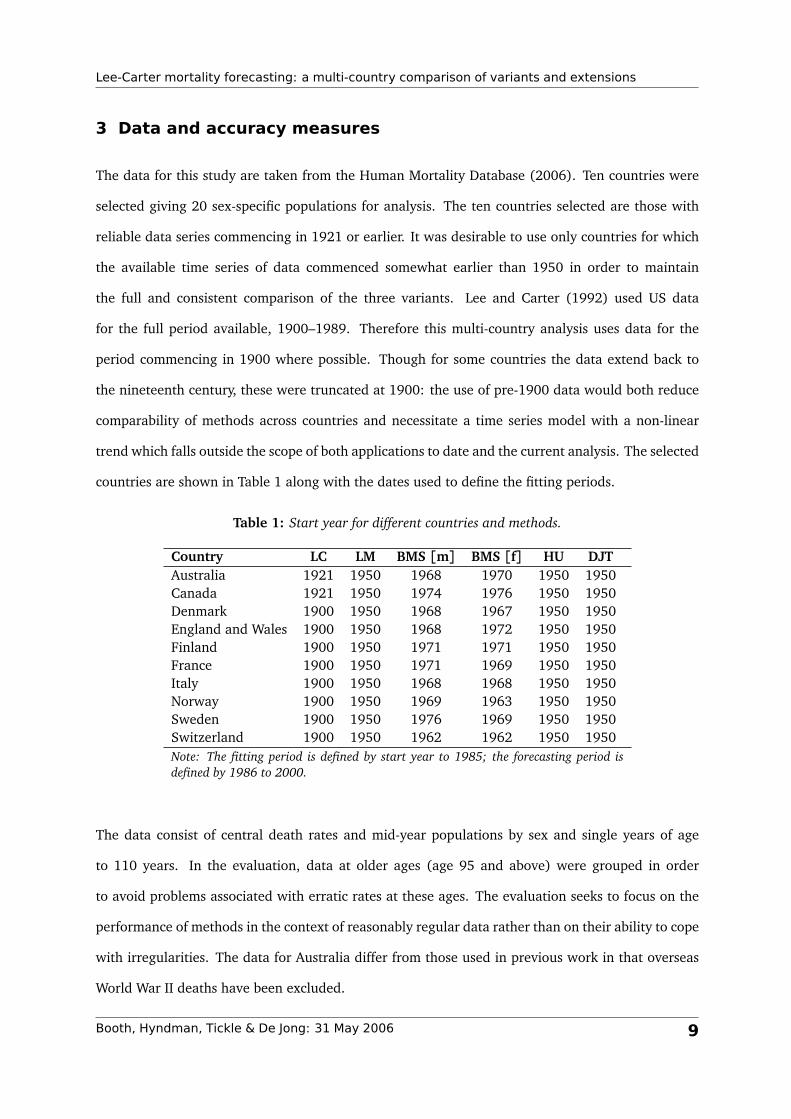
countries are shown in Table 1 along with the dates used to define the fitting periods.
Table 1: Start year for different countries and methods.
Country LC LM BMS [m] BMS [f] HU DJTAustralia 1921 1950 1968 1970 1950 1950Canada 1921 1950 1974 1976 1950 1950Denmark 1900 1950 1968 1967 1950 1950England and Wales 1900 1950 1968 1972 1950 1950Finland 1900 1950 1971 1971 1950 1950France 1900 1950 1971 1969 1950 1950Italy 1900 1950 1968 1968 1950 1950Norway 1900 1950 1969 1963 1950 1950Sweden 1900 1950 1976 1969 1950 1950Switzerland 1900 1950 1962 1962 1950 1950Note: The fitting period is defined by start year to 1985; the forecasting period isdefined by 1986 to 2000.
The data consist of central death rates and mid-year populations by sex and single years of age
to 110 years. In the evaluation, data at older ages (age 95 and above) were grouped in order
to avoid problems associated with erratic rates at these ages. The evaluation seeks to focus on the
performance of methods in the context of reasonably regular data rather than on their ability to cope
with irregularities. The data for Australia differ from those used in previous work in that overseas
World War II deaths have been excluded.
Booth, Hyndman, Tickle & De Jong: 31 May 2006 9
Lee-Carter mortality forecasting: a multi-country comparison of variants and extensions
The five methods were fitted to periods ending in 1985 and used to forecast death rates from 1986
to 2000. The methods are evaluated by comparing forecast log death rates with actual log death
rates.
Forecasting error in log death rates (forecast− actual) is averaged over forecast years, countries or
ages to give different views of the relative bias of the five methods. The absolute errors are also
averaged to provide measures of forecast accuracy. In addition to these errors in log death rates, the
error in life expectancy (forecast− actual) is examined. Again, these (and the absolute errors) are
averaged over countries or years to give different summary measures.
We investigate forecast bias in the methods using t-tests of zero mean applied to the errors in log
death rates averaged across forecast horizon and age. The sexes are treated separately. Similarly,
we test for zero mean in the errors in life expectancy averaged across forecast horizon.
4 Forecast evaluation of the five methods
We refer to the three Lee-Carter variants as LC, LM and BMS, and the two extensions as HU and
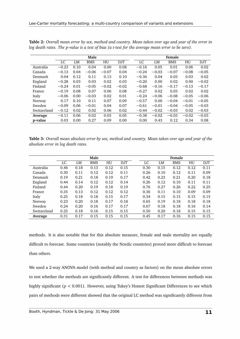
DJT. The overall mean errors for the 20 populations are shown in Table 2. The p-values in the
bottom row are based on t-tests of zero mean applied to the mean errors given in each column.
These results confirm earlier findings (Lee and Miller, 2001; Booth et al., 2005) that the original
Lee-Carter method consistently and substantially under-estimates mortality especially for females, as
indicated by the relatively large negative average errors. Results for the remaining four methods are
fairly similar, but only BMS and HU show no evidence of bias in either female or male mortality. Sex
differences in this measure are related to the cancellation of positive and negative errors (compare
Table 3).
Table 3 provides a summary of forecast accuracy based on mean absolute error. Again, LC performs
least well and there are only minor differences among the other four methods. It is notable that
the simple variations on the LC method used in LM and BMS provide substantial improvements
in forecast accuracy which are only marginally improved by the more sophisticated HU and DJT
Booth, Hyndman, Tickle & De Jong: 31 May 2006 10
Lee-Carter mortality forecasting: a multi-country comparison of variants and extensions
Table 2: Overall mean error by sex, method and country. Mean taken over age and year of the error inlog death rates. The p-value is a test of bias (a t-test for the average mean error to be zero).
methods. It is also notable that for this absolute measure, female and male mortality are equally
difficult to forecast. Some countries (notably the Nordic countries) proved more difficult to forecast
than others.
We used a 2-way ANOVA model (with method and country as factors) on the mean absolute errors
to test whether the methods are significantly different. A test for differences between methods was
highly significant (p < 0.001). However, using Tukey’s Honest Significant Differences to see which
pairs of methods were different showed that the original LC method was significantly different from
Booth, Hyndman, Tickle & De Jong: 31 May 2006 11
Lee-Carter mortality forecasting: a multi-country comparison of variants and extensions
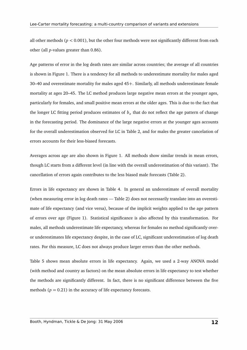
all other methods (p < 0.001), but the other four methods were not significantly different from each
other (all p-values greater than 0.86).
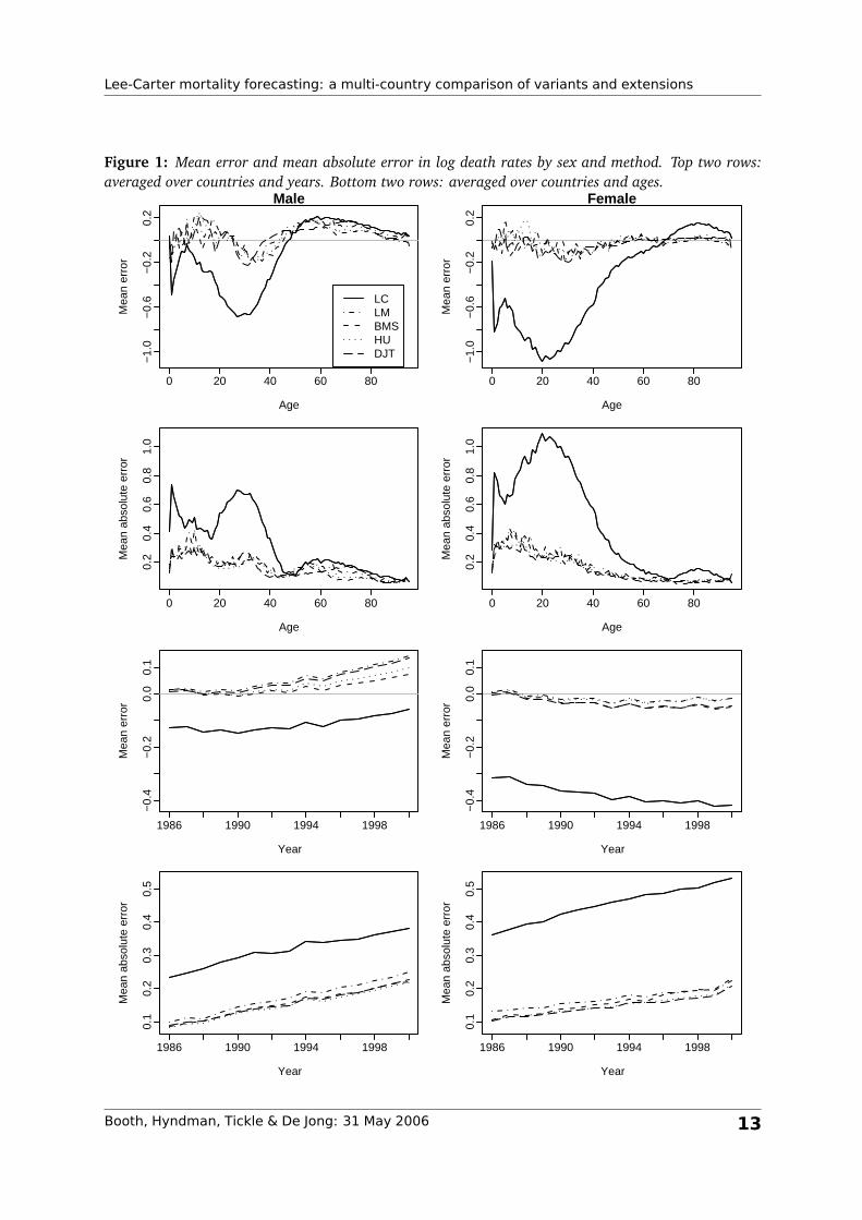
Age patterns of error in the log death rates are similar across countries; the average of all countries
is shown in Figure 1. There is a tendency for all methods to underestimate mortality for males aged
30–40 and overestimate mortality for males aged 45+. Similarly, all methods underestimate female
mortality at ages 20–45. The LC method produces large negative mean errors at the younger ages,
particularly for females, and small positive mean errors at the older ages. This is due to the fact that
the longer LC fitting period produces estimates of bx that do not reflect the age pattern of change
in the forecasting period. The dominance of the large negative errors at the younger ages accounts
for the overall underestimation observed for LC in Table 2, and for males the greater cancelation of
errors accounts for their less-biased forecasts.
Averages across age are also shown in Figure 1. All methods show similar trends in mean errors,
though LC starts from a different level (in line with the overall underestimation of this variant). The
cancellation of errors again contributes to the less biased male forecasts (Table 2).
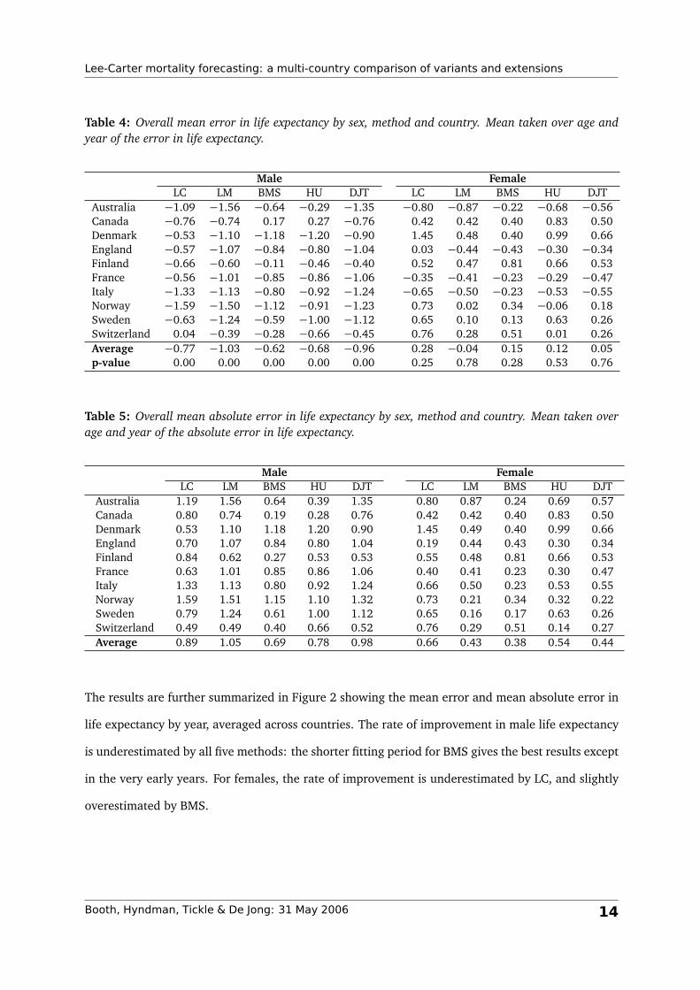
Errors in life expectancy are shown in Table 4. In general an underestimate of overall mortality
(when measuring error in log death rates — Table 2) does not necessarily translate into an overesti-
mate of life expectancy (and vice versa), because of the implicit weights applied to the age pattern
of errors over age (Figure 1). Statistical significance is also affected by this transformation. For
males, all methods underestimate life expectancy, whereas for females no method significantly over-
or underestimates life expectancy despite, in the case of LC, significant underestimation of log death
rates. For this measure, LC does not always produce larger errors than the other methods.
Table 5 shows mean absolute errors in life expectancy. Again, we used a 2-way ANOVA model
(with method and country as factors) on the mean absolute errors in life expectancy to test whether
the methods are significantly different. In fact, there is no significant difference between the five
methods (p = 0.21) in the accuracy of life expectancy forecasts.
Booth, Hyndman, Tickle & De Jong: 31 May 2006 12
Lee-Carter mortality forecasting: a multi-country comparison of variants and extensions
Figure 1: Mean error and mean absolute error in log death rates by sex and method. Top two rows:averaged over countries and years. Bottom two rows: averaged over countries and ages.
0 20 40 60 80
−1.
0−
0.6
−0.
20.
2
Male
Age
Mea
n er
ror
LCLMBMSHUDJT
0 20 40 60 80
−1.
0−
0.6
−0.
20.
2
Female
Age
Mea
n er
ror
0 20 40 60 80
0.2
0.4
0.6
0.8
1.0
Age
Mea
n ab
solu
te e
rror
0 20 40 60 80
0.2
0.4
0.6
0.8
1.0
Age
Mea
n ab
solu
te e
rror
1986 1990 1994 1998
−0.
4−
0.2
0.0
0.1
Year
Mea
n er
ror
1986 1990 1994 1998
−0.
4−
0.2
0.0
0.1
Year
Mea
n er
ror
1986 1990 1994 1998
0.1
0.2
0.3
0.4
0.5
Year
Mea
n ab
solu
te e
rror
1986 1990 1994 1998
0.1
0.2
0.3
0.4
0.5
Year
Mea
n ab
solu
te e
rror
Booth, Hyndman, Tickle & De Jong: 31 May 2006 13
Lee-Carter mortality forecasting: a multi-country comparison of variants and extensions
Table 4: Overall mean error in life expectancy by sex, method and country. Mean taken over age andyear of the error in life expectancy.
Table 5: Overall mean absolute error in life expectancy by sex, method and country. Mean taken overage and year of the absolute error in life expectancy.
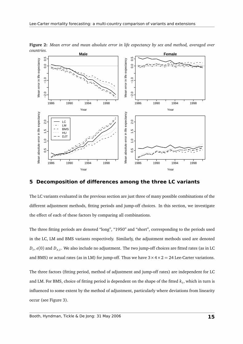
The results are further summarized in Figure 2 showing the mean error and mean absolute error in
life expectancy by year, averaged across countries. The rate of improvement in male life expectancy
is underestimated by all five methods: the shorter fitting period for BMS gives the best results except
in the very early years. For females, the rate of improvement is underestimated by LC, and slightly
overestimated by BMS.
Booth, Hyndman, Tickle & De Jong: 31 May 2006 14
Lee-Carter mortality forecasting: a multi-country comparison of variants and extensions
Figure 2: Mean error and mean absolute error in life expectancy by sex and method, averaged overcountries.
1986 1990 1994 1998
−2.
0−
1.0
0.0
0.5
Male
Year
Mea
n er
ror
in li
fe e
xpec
tanc
y
1986 1990 1994 1998
−2.
0−
1.0
0.0
0.5
Female
Year
Mea
n er
ror
in li
fe e
xpec
tanc
y
1986 1990 1994 1998
0.5
1.0
1.5
2.0
Year
Mea
n ab
solu
te e
rror
in li
fe e
xpec
tanc
y
LCLMBMSHUDJT
1986 1990 1994 1998
0.5
1.0
1.5
2.0
Year
Mea
n ab
solu
te e
rror
in li
fe e
xpec
tanc
y
5 Decomposition of differences among the three LC variants
The LC variants evaluated in the previous section are just three of many possible combinations of the
different adjustment methods, fitting periods and jump-off choices. In this section, we investigate
the effect of each of these factors by comparing all combinations.
The three fitting periods are denoted “long”, “1950” and “short”, corresponding to the periods used
in the LC, LM and BMS variants respectively. Similarly, the adjustment methods used are denoted
Dt , e(0) and Dx ,t . We also include no adjustment. The two jump-off choices are fitted rates (as in LC
and BMS) or actual rates (as in LM) for jump-off. Thus we have 3×4×2= 24 Lee-Carter variations.
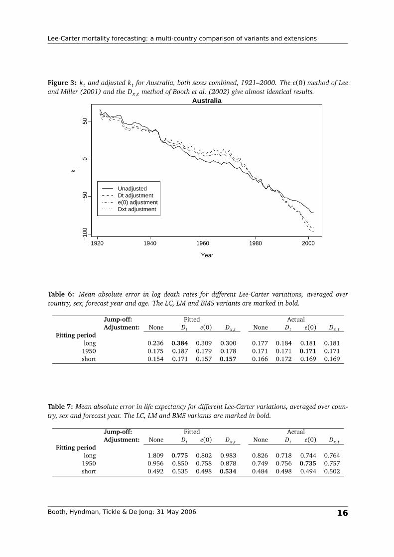
The three factors (fitting period, method of adjustment and jump-off rates) are independent for LC
and LM. For BMS, choice of fitting period is dependent on the shape of the fitted kt , which in turn is
influenced to some extent by the method of adjustment, particularly where deviations from linearity
occur (see Figure 3).
Booth, Hyndman, Tickle & De Jong: 31 May 2006 15
Lee-Carter mortality forecasting: a multi-country comparison of variants and extensions
Figure 3: kt and adjusted kt for Australia, both sexes combined, 1921–2000. The e(0) method of Leeand Miller (2001) and the Dx ,t method of Booth et al. (2002) give almost identical results.
Table 6: Mean absolute error in log death rates for different Lee-Carter variations, averaged overcountry, sex, forecast year and age. The LC, LM and BMS variants are marked in bold.
Table 7: Mean absolute error in life expectancy for different Lee-Carter variations, averaged over coun-try, sex and forecast year. The LC, LM and BMS variants are marked in bold.