ISSN 1471-0498

DEPARTMENT OF ECONOMICS

DISCUSSION PAPER SERIES

PRODUCTIVITY ANALYSIS IN GLOBAL MANUFACTURING PRODUCTION

Markus Eberhardt and Francis Teal

Number 515 November 2010

Manor Road Building, Oxford OX1 3UQ

PRODUCTIVITY ANALYSIS IN

GLOBAL MANUFACTURING PRODUCTION∗

Markus Eberhardta,b† Francis Tealb,c

a St Catherine’s College, Oxford

b Centre for the Study of African Economies,

Department of Economics, University of Oxford

c Institute for the Study of Labor (IZA), Bonn

Job Market Paper

This version: 2nd November 2010

Abstract: Despite the widely recognised importance of the manufacturing industry for success-ful development few studies investigate this sector in cross-country analysis. We fill this gap inthe literature by analysing manufacturing production across a large number of developing anddeveloped economies. Our empirical framework allows for heterogeneous production technologyand accounts for endogeneity as well as cross-section dependence in the panel. Our resultsimply that differences in production technology are of crucial importance for understandingcross-country differences in labour productivity and their underlying causes. In the light ofthese findings the interpretation of regression intercepts as TFP level estimates collapses andwe introduce an alternative measure which is robust to parameter heterogeneity.

Keywords: Cross-Country Analysis; Parameter Heterogeneity; Productivity Levels; PanelTime Series Econometrics; Common Factor Model

JEL classification: C23, O14, O47

∗We are grateful to Michael Binder, Steve Bond, Steven Durlauf, David Hendry, John Muellbauer, HashemPesaran, Ron Smith and Jonathan Temple for helpful comments and suggestions. We further benefited fromcomments during presentations at the 2nd Advanced Summer School at the Department of Economics of theUniversity of Crete, the Gorman Student Research Workshop and the Productivity Workshop, University of Ox-ford, the Nordic Conference for Development Economics in Stockholm, the Economic & Social Research Council(ESRC) Development Economics conference in Brighton, the International Conference for Factor Structures forPanel and Multivariate Time Series Data in Maastricht and the DEGIT XV conference in Frankfurt. All remain-ing errors are our own. This document is an output from research funded by the UK Department for InternationalDevelopment (DfID) as part of the iiG, a research programme to study how to improve institutions for pro-poorgrowth in Africa and South-Asia. The first author further acknowledges financial support from the ESRC [grantnumbers PTA-031-2004-00345 and PTA-026-27-2048]. The views expressed are not necessarily those of DfID orthe ESRC.†Correspondence: Centre for the Study of African Economies (CSAE), Department of Economics, Uni-

versity of Oxford, Manor Road Building, Manor Road, Oxford OX1 3UQ, United Kingdom. Email:markus.eberhardt@economics.ox.ac.uk. Tel.: +44 (0)1865 271084, Fax: +44 (0)1865 281447.

1

1 Introduction

The central importance of the manufacturing sector for successful development has become awidely recognised ‘stylised fact’ in development economics. Yet in contrast to the literature oncross-country growth regressions using aggregate economy data (see survey by Durlauf, Johnsonand Temple, 2005) there is limited empirical work dedicated to the analysis of the manufacturingsector in a large cross-section of countries — with the notable exception of Martin and Mitra(2002), cross-country empirical analysis at the sectoral level is typically based on Total FactorProductivity (TFP) accounting and/or limited to OECD countries (Bernard and Jones, 1996a;Harrigan, 1999; Malley, Muscatelli and Woitek, 2003; Hultberg, Nadiri and Sickles, 2004). Ifmanufacturing matters for development it seems self-evidently important to learn about theproduction process and its drivers in this industrial sector.

In this paper we attempt to fill this gap in the literature by estimating cross-country productionfunctions for the manufacturing sector in 48 developing and developed countries using annualdata from 1970 to 2002 (UNIDO, 2004). Building on earlier work on growth empirics (Eberhardtand Teal, 2010) we show that technology differences are of crucial importance for understand-ing cross-country differences in labour productivity and their causes (Durlauf, Kourtellos andMinkin, 2001). Note that we refer to heterogeneity in ‘technology parameters’ to indicate dif-ferential production parameters on observable and unobservable inputs across countries, notmerely country-specific TFP growth terms. This aside our study emphasises the importance oftime-series properties of inputs and TFP (Nelson and Plosser, 1982; Bernard and Jones, 1996b;Funk and Strauss, 2003; Bond, Leblebicioglu and Schiantarelli, 2010) as well as of accounting forcross-section correlation in the panel (Moscone and Tosetti, 2009; Chudik, Pesaran and Tosetti,2010; Sarafidis and Wansbeek, 2010).1 We adopt a common factor modelling framework (Baiand Ng, 2004; Pesaran, 2006; Bai, 2009b; Kapetanios, Pesaran and Yamagata, 2010) and employempirical estimators that can accommodate all of the above matters (Pesaran, 2006; Bond andEberhardt, 2009).2

Our findings have important implications for productivity analysis both at the sectoral and theaggregate economy level: first, like firms in different industries, different countries are char-acterised by different production technologies. Our study shows that attempts at estimatingcross-country production functions in pooled models, where by construction the same technol-ogy applies in all countries, are fundamentally misspecified and yield biased estimates for thetechnology parameters and thus any TFP estimates derived from them. Second, merely allowingfor technology heterogeneity is also insufficient to capture the complex production process atthe country-level: in a globalising world economies interact through trade, cultural, politicaland other ties and at the same time are affected differentially by global phenomena such as therecent financial crisis or the emergence of China as a major economic player. This creates aweb of interdependencies within and across economies, leading to the breakdown of standardpanel estimators employed in the existing cross-country studies. Our empirical strategy accom-modates this interplay of endogeneity, heterogeneity and commonality to provide evidence forthe fundamental forces driving manufacturing development across the globe. Third, followingon from these findings the conventional interpretation of regression intercepts as TFP levelestimates breaks down once production technology is allowed to differ across countries. We in-troduce an alternative methodology for TFP level determination which is robust to this featureand provide an analysis for the manufacturing case.

1Empirical productivity analysis which allows for cross-section dependence is still relatively limited, e.g. pro-duction functions for Italian regions (Costantini and Destefanis, 2009) or Chinese provinces (Fleisher, Li andZhao, 2010).

2In order to avoid confusion with the ‘common factor model’ terminology we refer to ‘factor inputs’ (i.e. thefactors of production, labour and capital) simply as inputs. Whenever we talk of ‘factors’ we mean to refer to ft.

2

The analysis here represents a step toward making cross-country empirics relevant to individualcountries by moving away from empirical results that characterise the average country andtoward a deeper understanding of the differences (Ranis and Fei, 1988), a notion which is clearlyechoed elsewhere in the literature (Quah, 1997; Temple, 1999; Durlauf, 2001; Durlauf et al., 2001,2005). Cross-country regressions of time averages, in the neoclassical tradition of Barro (1991)and Mankiw, Romer and Weil (1992), emphasise the variation in the data across countries(‘between variation’) and implicitly assume that the processes driving capital accumulation in,say, the United States are the same as those in Malawi, and that at a distant point in timethe latter can feasibly reach the capital-labour ratio of the former to achieve the same levelof development. However, this is not how development takes place. Instead, the very word‘development’ suggests an evolution over time, which requires that apart from recognising thepotential for differences across countries we analyse the individual evolution paths of countriesover time (thus emphasising the ‘within variation’ in the data). The empirical methods used inthis paper enable us to incorporate all of these concerns within one unifying empirical framework.At present our results only allow for technology differences across countries. Future work in thisarea will have to follow the call toward an integrated treatment of the production technology inits entirety, which is able “to explain why this parameter heterogeneity exists” (Durlauf et al.,2001, p.935).

The remainder of the paper is structured as follows: in the first part of the paper in Sections 2 to4 we concern ourselves with the conceptual motivation, set out the empirical model and discussempirical implementation. In the second part in Section 5 we introduce the data and presentour empirical results. The third part in Section 6 covers the implications of these findings forconventional TFP determination in the parametric literature, providing a simple alternativemethodology. Section 7 concludes.

2 Modelling technology over time and across countries

In this section we motivate the concerns with which we approach the estimation of cross-countryproduction functions. Technology heterogeneity as well as the time-series and cross-sectioncorrelation properties of macro panel data have not been considered in great detail in theempirical growth literature (Durlauf and Quah, 1999; Temple, 1999; Durlauf et al., 2005), buthave solid foundations in the theoretical literatures on growth and econometrics. We discusseach of these issues in some more details in the following.

A theoretical justification for heterogeneous technology parameters can be found in the ‘newgrowth’ literature. This strand of the theoretical growth literature argues that productionfunctions differ across countries and seeks to determine the sources of this heterogeneity (Durlaufet al., 2001). Intuitively, the heterogeneity in production technology could be taken to mean thatcountries can choose an ‘appropriate’ production technology from a menu of feasible options.The model by Azariadis and Drazen (1990) can be seen as the ‘grandfather’ for many of thetheoretical attempts to allow countries to possess different technologies from each other. Theirmodel incorporates a qualitative change in the production function, whereby upon reaching acritical ‘threshold’ of human capital, economies will jump to a higher steady-state equilibriumgrowth path represented by a different production function. Further theoretical work leadsto multiple equilibria interpretable as differential production technology across countries (e.g.Murphy, Shleifer and Vishny, 1989; Durlauf, 1993; Banerjee and Newman, 1993). A simplerjustification for heterogeneous production functions is offered by Durlauf et al. (2001), namelythat the Solow model was never intended to be valid in a homogeneous specification for allcountries, but may still be a good way to investigate each country, i.e. if we allow for parameterdifferences across countries.

3

In the long-run, variable series such as value-added or capital stock often display high levels ofpersistence, such that it is not unreasonable to suggest for these series to be ‘nonstationary’processes in some countries (Nelson and Plosser, 1982; Granger, 1997; Lee, Pesaran and Smith,1997; Rapach, 2002; Bai and Ng, 2004; Pedroni, 2007; Canning and Pedroni, 2008). Althougheconomic time-series in practice are usually not precisely integrated of any given order, it isfor our purposes sufficient to assume that nominal and real value series typically behave asI(2) and I(1) respectively (Hendry, 1995; Jones, 1995). Pedroni has suggested that variable(non)stationarity should not be seen as a ‘global’ property, valid for all times, but as a “featurewhich describes local behaviour of the series within sample” (Pedroni, 2007, p.432).

In our general empirical model we emphasise a view of TFP as a ‘measure of our ignorance’(Abramowitz, 1956), incorporating a wider set of factors that can shift the production possibilityfrontier (for instance “resource endowments, climate, institutions, and so on”, Mankiw et al.,1992, p.410/1). This is in contrast to the notion of TFP as a definitive efficiency index, ascommonly adopted in the microeconometric literature on production analysis. Furthermore,it is important to allow for the possibility that TFP is in part common to all countries, e.g.representing the global dissemination of non-rival scientific knowledge or global shocks, suchas the recent financial crisis or the 1970s oil crises. Alternatively, we can think of multipleeconomic, social, political and cultural ties between countries from which commonality (cross-section correlation) may arise. The individual evolution paths of the unobservables making upTFP should feasibly not be restrained to follow simple linear trends, but instead be allowedto evolve in a non-linear and even nonstationary fashion. For instance, a number of empiricalpapers report that their measures of TFP display nonstationarity, whether analysed at theeconomy level (Coe and Helpman, 1995; Coe, Helpman and Hoffmaister, 1997; Kao, Chiangand Chen, 1999; Engelbrecht, 2002; Bond, Leblebicioglu and Schiantarelli, 2007) or at thesectoral level (Bernard and Jones, 1996b; Funk and Strauss, 2003). Further, Coakley, Fuertesand Smith (2006) state explicitly with reference to cross-country production function estimationthat technology shocks are plausibly nonstationary. At the same time a highly flexible approachto empirical modelling using annual data raises the question of how business cycles influenceor distort the empirical estimates (Eberhardt and Teal, 2010). All of these concerns point tothe adoption of a multi-factor TFP structure that allows for common as well as country-specificelements. We implement this structure by using the uniquely suited common factor modellingframework (Bai, 2009b).

Taking these insights about heterogeneity, cross-section dependence and nonstationarity at facevalue one may then suggest that the macro production process is representative of a cointe-grating relationship between output and ‘some set of inputs’, likely including TFP (Pedroni,2007; Canning and Pedroni, 2008). Our analysis here will incorporate an investigation of thecointegration properties of production inputs and TFP in the long-run equilibrium produc-tion function. It is important to note that existing empirical work has primarily concerneditself with the (potential) endogeneity of regressors in the empirical framework (e.g. Caselli,Esquivel and Lefort, 1996; Bond, Hoeffler and Temple, 2001), an issue that is given consider-ably more attention in the literature than the data properties or the potential misspecificationof the empirical regression model. While the empirical methods adopted here can address thesimultaneity between TFP shocks and input accumulation, we need to resort to an alterna-tive estimation approach following Pedroni (2001) to rule out the potential of reverse causalityand assure us that our regressions represent production function models and not investment orlabour demand equations in disguise. Thus in addition to incorporating much desirable tech-nology heterogeneity, our empirical analysis addresses all the concerns that have occupied thestandard literature.

4

3 Empirical framework

We adopt a common factor representation for a standard log-linearised Cobb-Douglas produc-tion function model: for i = 1, . . . , N , t = 1, . . . , T and m = 1, . . . , k let

yit = β′i xit + uit uit = αi + λ′i ft + εit (1)xmit = πmi + δ′mi gmt + ρ1mi f1mt + . . .+ ρnmi fnmt + vmit (2)

ft = %′ft−1 + εt and gt = κ′gt−1 + εt (3)

where f ·mt ⊂ ft. yit represents value-added and xit is a vector of observable inputs includinglabour and capital stock (all in logarithms). For unobserved TFP we employ the combinationof a country-specific TFP level αi and a set of common factors ft with country-specific factorloadings λi — TFP is thus in the spirit of a ‘measure of our ignorance’ (Abramowitz, 1956) andoperationalised via an unobserved common factor representation. In equation (2) we providean empirical representation of the k observable input variables, which are modeled as linearfunctions of the unobserved common factors ft and gt, with country-specific factor loadingsrespectively. The model setup thus introduces cross-section dependence in the observables andunobservables. As can be seen, some of the unobserved common factors driving the variationin yit in equation (1) also drive the regressors in (2). This setup leads to endogeneity wherebythe regressors are correlated with the unobservables of the production function equation (uit),making it difficult to identify βi separately from λi and ρi (Kapetanios et al., 2010).3 Technologyparameters βi can differ across countries but are assumed constant over time.4 Equation (3)specifies the evolution of the unobserved factors, which includes the potential for nonstationaryfactors (% = 1, κ = 1) and thus nonstationary inputs and output variables. Note that thecommon factor framework is sufficiently general to allow for common and heterogeneous businesscycles which are commonly seen to distort empirical analysis using annual data.5

The three most important features of the above setup are the potential nonstationarity ofobservables and unobservables (yit, xit, ft, gmt), the potential heterogeneity in the impact ofobservables and unobservables on output across countries (αi, βi, λi) as well as the endogeneityof observable input variables created by the common factor structure. These properties haveimportant bearings on estimation and inference in macro panel data which are at the heart ofthis paper.

4 Empirical implementation

The matters of parameter heterogeneity, data time-series properties and cross-section depen-dence in empirical analysis using macro panel data are developed at great length elsewhere(Eberhardt and Teal, 2010). In this section we therefore restrict ourselves to the discussion ofthe identification problem highlighted above, before we introduce two estimators which allowfor heterogeneity in the impact of observables and unobservables.

3Note that the common factor setup is transferable to the micro-level setup where Arellano and Bond (1991);Blundell and Bond (1998) and Levinsohn and Petrin (2003) (amongst others) are concerned about ‘unobservedproductivity shocks’ (see Bai, 2009a).

4The latter assumption is clearly restrictive, but given the focus on cross-country technology heterogeneityagainst the background of data restrictions in the time-series dimension we cannot relax this assumption for theheterogeneous regression models. For the pooled models we ran separate regressions using pre- and post-1985subsamples for the value-added models. Estimates for POLS, CCEP and FD-OLS are virtually identical for thetwo sub-periods. Period estimates for the FE estimator differ somewhat but the 95% confidence intervals stillshow considerable overlap.

5For details see Eberhardt and Teal (2010, Section 4).

5

If we assume factors ft (and gmt) in our general model above are stationary, the consistency ofstandard panel methods such as a pooled Fixed Effects or a Pesaran and Smith (1995) MeanGroup estimator rests on the factor loadings of the unobserved common factors contained inboth the y and x-equations (λi, ρi): if their averages are jointly non-zero a regression of y on xand N intercepts will be subject to the omitted variable problem and hence misspecified, sinceregression error terms will be correlated with the regressor, leading to biased estimates andincorrect inference (Coakley et al., 2006; Pesaran, 2006). In the case of nonstationary factorsthe consistency issues are altogether more complex and will depend on the exact specificationof the model. However, regardless of their order of integration, standard estimation approachesneglecting common factors will not yield an estimate of β or the mean of βi, but of βi +λiρ−1

i ,as shown by Kapetanios et al. (2010): βi is unidentified. Under the specification described, astandard pooled Fixed Effects or Pesaran and Smith (1995) Mean Group estimator will thereforelikely yield an inconsistent estimator (due to residual nonstationarity) of a parameter we arenot interested in (due to the identification problem).

Our empirical approach emphasises the importance of parameter and factor loading heterogene-ity across countries. The following 2×2 matrix indicates how the various estimators implementedbelow account for these matters.6 We abstract from discussing the standard panel estimatorshere and refer to the overview article by Coakley et al. (2006), as well as the articles by Pedroni(2000, 2001) for more details.

Factor loadings:Technology parameters: homogeneous heterogeneous

homogeneous POLS, FE, FD-OLS CCEP

heterogeneous MG, RCM, GM-FMOLS CMG, AMG, ARCM

Essentially, in our model setup all estimators neglecting the heterogeneity in unobservables(left column) suffer from the identification problem described above. In addition, the time-series properties of both observable and unobservable processes create further difficulties forestimation and inference in these empirical approaches as errors may be nonstationary. Inferenceis problematic in this case since conventional standard errors will be invalid (Kao, 1999). Amongthese estimators the Pedroni (2000) GM-FMOLS is the only one avoiding this issue by adoptinga nonstationary panel econometric approach relying on cointegrated variables.

The estimators allowing for heterogeneity in factor loadings adopted here (right column) operatethrough augmenting the regression equation(s) with ‘proxies’ or estimates for the unobservedcommon factors. This augmentation avoids the identification problem and is also an appro-priate strategy to account for other cross-section dependence, e.g. spatial correlation, in thepresence of nonstationary variables (Pesaran and Tosetti, 2010; Chudik et al., 2010; Kapetan-ios et al., 2010). The Pesaran (2006) CCE estimators account for the presence of unobservedcommon factors by including cross-section averages of the dependent and independent variablesin the regression equation — in the pooled version (CCEP) these averages are interacted withcountry-dummies to allow for country-specific parameters, whereas in the heterogeneous ver-sion (CMG) this is achieved by construction and the estimates are obtained as averages of theindividual country estimates, following the Pesaran and Smith (1995) MG approach. A relatedapproach which we term the Augmented Mean Group (AMG) estimator accounts for cross-section dependence by inclusion of a ‘common dynamic process’ in the country regression. This

6Abbreviations: POLS — Pooled OLS, FE — Fixed Effects, FD-OLS — OLS with variables in first differences,MG — Pesaran and Smith (1995) Mean Group, RCM — Swamy (1970) Random Coefficient Model, GM-FMOLS— Pedroni (2000) Group-Mean Fully Modified OLS, CCEP/CMG — Pesaran (2006) Common Correlated Effectsestimators, and AMG/ARCM — Augmented MG and RCM, described in detail below. Note that our FEestimator (like the OLS and FD-OLS) is augmented with T −1 year dummies such that it is in effect a ‘Two-WayFixed Effects’ (2FE) estimator.

6

process is extracted from the year dummy coefficients of a pooled regression in first differences(FD-OLS) and represents the levels-equivalent mean evolution of unobserved common factorsacross all countries. Provided the unobserved common factors form part of the country-specificcointegrating relation (Pedroni, 2007), the augmented country regression model encompassesthe cointegrating relationship, which is allowed to differ across i.

Stage (i) ∆yit = b′∆xit +T∑t=2

ct∆Dt + eit ⇒ ct ≡ µ•t (4)

Stage (ii) yit = ai + b′ixit + cit+ diµ

•t + eit bAMG = N−1

∑i

bi (5)

Stage (i) represents a standard FD-OLS regression with T −1 year dummies in first differences,from which we collect the year dummy coefficients (relabelled as µ•t ). This process is extractedfrom the pooled regression in first differences since nonstationary variables and unobservablesare believed to bias the estimates in the pooled levels regressions. In stage (ii) µ•t is includedin each of the N standard country regressions which also include a linear trend term to captureomitted idiosyncratic processes evolving in a linear fashion over time. Alternatively we cansubtract µ•t from the dependent variable, which implies the common process is imposed on eachcountry with unit coefficient. In either case estimates are averaged across countries following thePesaran and Smith (1995) MG approach. Based on the results of Monte Carlo simulations (Bondand Eberhardt, 2009) we posit that the inclusion of µ•t allows for the separate identification ofβi or E[βi] and the unobserved common factors driving output and inputs, like in the Pesaran(2006) CCE approach. In analogy, we can use ∆µ•t in the country equations in first differencesand can augment the Swamy (1970) RCM estimator in a similar fashion to yield the AugmentedRandom Coefficient Model (ARCM) estimators in levels and first differences — results for theARCM were very similar to those in the AMG and in the interest of space are therefore omittedin the empirical section. We also applied an alternative version of the estimator where the firststage allows for heterogeneous slopes across countries: results for the AMG second stage arenext to identical to those presented in Table 2.

The focus of the CCE estimators is the estimation of consistent b and not the nature of theunobserved common factors or their factor loadings: we cannot obtain an explicit estimate forthe unobserved factors ft or the factor loadings λi, since the average impact of the factors (λ)is unknown. Our augmented estimators use an explicit rather than implicit estimate for ft fromthe pooled first stage regression. Compared with the CCE approach we can obtain a simplebut economically meaningful construct from the AMG setup: the common dynamic processµ•t = h(λft) represents common TFP evolution over time, whereby common is defined either inthe literal sense, or as the sample mean of country-specific TFP evolution. The country-specificcoefficient on the common dynamic process, di from equation (5), represents the implicit factorloading on common TFP.

Immediate concerns about this augmented estimator relate to the issue of second stage ‘re-gressions with generated regressors’ (Pagan, 1984). However, simulation results (Bond andEberhardt, 2009) suggest that the average standard error of the AMG estimates is of similarmagnitude to the empirical standard deviation. A theoretical explanation is provided in Baiand Ng (2008), who show that second stage standard errors need not be adjusted for first stageestimation uncertainty if

√T/N → 0, as is arguably the case here.

7

5 Data and main empirical results

5.1 Data

For our empirical analysis we employ aggregate sectoral data for manufacturing from developedand developing countries for the period 1970 to 2002 (UNIDO, 2004). Our sample represents anunbalanced panel of 48 countries with an average of 24 time-series observations (min: 11, max:33). A detailed discussion of the data and descriptive statistics can be found in the Appendix.All of the results presented are strikingly robust to the use of a reduced sample constructedwith application of a set of rigid ‘cleaning’ rules. Furthermore, we carried out all regressionsbelow in a gross-output model with materials as additional input — VA-equivalent results arevirtually identical to those presented here (detailed results available on request).

5.2 Time-series properties of the data

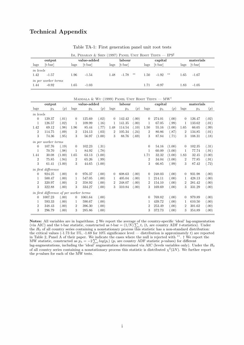
We carried out a range of stationarity and nonstationarity tests for individual country time-series as well as the panel as a whole (full results available on request). The panel unit roottests conducted include first (Im, Pesaran and Shin, 1997; Maddala and Wu, 1999) and sec-ond generation procedures (Pesaran, 2007) — see Technical Appendix. In case of the presentdata dimensions and characteristics, and given all the problems and caveats of individual coun-try unit root tests as well as panel unit root tests, we can suggest most conservatively thatnonstationarity cannot be ruled out in this dataset.

5.3 Pooled regressions

We estimate pooled models with variables in levels or first differences, including T − 1 yeardummies or country-specific period-averages a la Pesaran (2006). By construction, the slopecoefficients on the inputs in these models are restricted to be the same across all countries. Ourresults are presented in Table 1, with unrestricted models and models with CRS imposed in theupper and lower panel respectively.

Estimates for the input parameters in the regressions without any restrictions on the returnsto scale are statistically significant at the 5% level or 1% level. The POLS results in [1] suggestthat failure to account for time-invariant heterogeneity across countries (fixed effects) yieldsbiased results: at around .8 the capital coefficient is considerably inflated. Inclusion of countryintercepts in [2] reduces these coefficient estimates somewhat. The same parameter in the CCEPresults in [3] is yet lower still, around .6. In both the FE and CCEP estimators the fixed effectsare highly significant (F -tests reported in the Table footnote). For all three estimators in levelsthe regression diagnostics suggest serial correlation in the error terms, while constant returnsto scale are rejected at the 1% level of significance except for POLS. Note that for the FEestimator the data rejects CRS in favour of increasing returns — an unusual finding. The OLSregressions in first differences in [4] yield somewhat different technology estimates: the capitalcoefficient is now around .3 in both specifications. CRS cannot be rejected, the AR(1) testsshow serial correlation for this model, which is to be expected given that errors are now in firstdifferences. There is however evidence of some higher order autocorrelation.7

7Note that we obtain identical results for models in [1], [2] and [4] if we use data in deviation from the cross-sectional mean (results not presented) instead of using a set of year dummies. Replacing year dummies withcross-sectionally demeaned data is only valid if parameters are homogeneous across countries (Pedroni, 1999,2000).

8

Table 1: Static pooled regressions

Panel (A): Unrestricted Returns to Scale

[1] [2] [3] [4]estimator POLS FE CCEP FD

dependent variable lY lY lY ∆lY

log labour 0.2100 0.4402 0.6009[12.08]∗∗ [17.43]∗∗ [19.48]∗∗

∆log labour 0.6849[7.43]∗∗

log capital 0.7896 0.7174 0.6144[67.34]∗∗ [32.17]∗∗ [22.76]∗∗

∆log capital 0.3463[3.40]∗∗

intercept 1.1510 -0.0470 -0.5160[7.99]∗∗ [0.13] [0.98]

CRS: F .96 .00 .00 .72FE: F .00 .00AR(1) .00 .00 .00 .00AR(2) .00 .00 .00 .01I(1) 1.00 1.00 .00 .00RMSE .462 .130 .102 .103

Panel (B): CRS imposed

[1] [2] [3] [4]estimator POLS FE CCEP FD

dependent variable ly ly ly ∆ly

log capital pw 0.7895 0.6752 0.5823[72.97]∗∗ [29.89]∗∗ [23.38]∗∗

∆log capital pw 0.3195[3.61]∗∗

intercept 1.1474 2.3786 0.2489[8.47]∗∗ [9.98]∗∗ [0.63]

FE: F .00 .00AR(1) .00 .00 .00 .00AR(2) .00 .00 .00 .01I(1) 1.00 .78 .00 .00RMSE .462 .135 .113 .103

Notes: Values in brackets are absolute t-statistics, based on White heteroskedasticity-consistent standarderrors. We indicate statistical significance at the 5% and 1% level by ∗ and ∗∗ respectively. Regressions are forN = 48 countries, n = 1, 194 (n = 1, 128) observations in the levels (first difference) regressions. Dependentvariables: lY (ly) — log value-added (per worker), ∆lY(∆ly) — growth rate of value-added (per worker). Forthe CCEP estimator we include sets of cross-section period averages of value-added, labour, and capital stock(in the CRS equations the respective variables in per worker terms), all in logs (estimates not reported) — seePesaran (2006) for details. All other models include T − 1 year dummies in levels or FD (estimates notreported). For all diagnostic tests (except RMSE) we report p-values: (i) The null hypothesis for the Wald testsis constant returns. (ii) The F -tests in the FE and CCEP regressions reject the null that fixed effects do notdiffer across countries. (iii) The Arellano and Bond (1991) AR test on the residuals has the null of no serialcorrelation. (iv) ‘I(1)’ reports results for a Pesaran (2007) CIPS test with 2 lags, null of nonstationarity (fullresults available on request). (v) RMSE is the root mean squared error.

9

Under intercept and technology parameter heterogeneity, given nonstationarity in (some of) thecountry variable series the pooled FE estimates in column [2] asypmtotically converge to the‘long-run average’ relation at speed

√N (Phillips and Moon, 1999) provided T/N → 0 (joint

asymptotics) and cross-section independence. In the present sample, however, nonstationaryerror terms and unobserved common factors seem to influence the results considerably: a capitalcoefficient of around .7 is more than twice the magnitude of the macro data on factor shares inincome (Mankiw et al., 1992; Gomme and Rupert, 2004), a common finding in the literature(Islam, 2003; Pedroni, 2007). Further recall that t-ratios are invalid for the estimations in levelsif error terms are nonstationary (Kao, 1999; Coakley, Fuertes and Smith, 2001). The CCEPestimator accounts for cross-section dependence and the residual analysis suggests, stationaryerrors terms. The difference estimator in [4] converges to the common cointegrating vector β orβ or the mean of the individual country cointegrating relations, E[βi], at speed

√TN (Smith and

Fuertes, 2007). investigation regarding alternative specification with parameter heterogeneityas well as residual diagnostics will be necessary to judge the bias of the CCEP results.

Our pooled regression analysis suggests that time-series properties of the data play an importantrole in estimation: we suggest that the bias in the levels models is the result of nonstationaryerrors, which are introduced into the pooled OLS and FE equations by the imposition of pa-rameter homogeneity. In contrast, the FD-OLS regressions where variables are stationary yieldmore sensible capital parameters. This pattern of results fits the case of I(1) level-series in atleast some of the countries in our sample. The results for the CCEP are somewhat surprisingand we would speculate that these are driven by outliers.

5.4 Common TFP

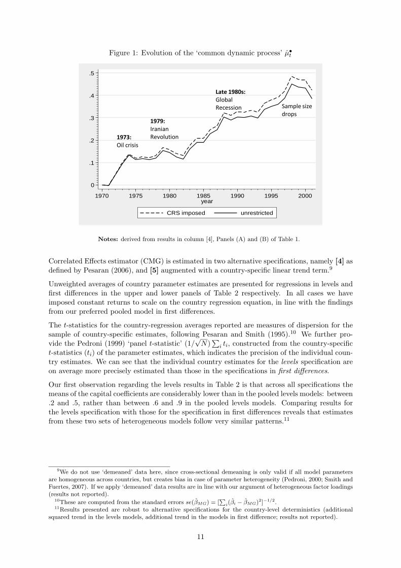
Following our argument above, the FD-OLS regression represents the only pooled regressionmodel which estimates a cross-country average relationship safe from difficulties introduced bynonstationarity. We therefore make use of the year dummy coefficients derived from our pre-ferred pooled model to obtain an estimate of the common dynamic process µ•t , which representsan estimate of the common TFP evolution. Figure 1 illustrates the evolution path of thiscommon dynamic process for the unrestricted and CRS models.

The graphs show severe slumps following the two oil shocks in the 1970s, while the 1980s and1990s indicate considerable upward movement.8 If we follow the ‘measure of our ignorance’interpretation of TFP, then a decline in global manufacturing TFP as evidenced in the 1970sshould not be interpreted as a decline in knowledge, but a worsening global manufacturingenvironment, which seems plausible. An alternative explanation may be that our variabledeflation does not adequately capture all the price changes in general, and material input pricechanges vis-a-vis output prices in particular, occurring in the post-oil shock periods.

5.5 Country regressions

In the following we relax the assumption implicit in the pooled regressions that all countriespossess the same production technology. At the same time, we maintain that common shocksand/or cross-sectional dependence have to be accounted for in some fashion. We consider: [1]the standard Pesaran and Smith (1995) Mean Group (MG) estimator; the Augmented MeanGroup (AMG) estimator either [2] with the common dynamic process (µ•t ) imposed with unitcoefficient, or [3] included as additional regressor. The Mean Group version of the Common

8These graphs are ‘data-specific’: for years where data coverage is good, this can be interpreted as ‘global’,whereas in later years (10 countries have data for 2001, only 2 for 2002, omitted from the graph) this interpretationcollapses.

10

Figure 1: Evolution of the ‘common dynamic process’ µ•t

0

.1

.2

.3

.4

.5

1970 1975 1980 1985 1990 1995 2000year

CRS imposed unrestricted

1973:Oil crisis

1979: Iranian Revolution

Late 1980s: Global Recession Sample size

drops

Notes: derived from results in column [4], Panels (A) and (B) of Table 1.

Correlated Effects estimator (CMG) is estimated in two alternative specifications, namely [4] asdefined by Pesaran (2006), and [5] augmented with a country-specific linear trend term.9

Unweighted averages of country parameter estimates are presented for regressions in levels andfirst differences in the upper and lower panels of Table 2 respectively. In all cases we haveimposed constant returns to scale on the country regression equation, in line with the findingsfrom our preferred pooled model in first differences.

The t-statistics for the country-regression averages reported are measures of dispersion for thesample of country-specific estimates, following Pesaran and Smith (1995).10 We further pro-vide the Pedroni (1999) ‘panel t-statistic’ (1/

√N)

∑i ti, constructed from the country-specific

t-statistics (ti) of the parameter estimates, which indicates the precision of the individual coun-try estimates. We can see that the individual country estimates for the levels specification areon average more precisely estimated than those in the specifications in first differences.

Our first observation regarding the levels results in Table 2 is that across all specifications themeans of the capital coefficients are considerably lower than in the pooled levels models: between.2 and .5, rather than between .6 and .9 in the pooled levels models. Comparing results forthe levels specification with those for the specification in first differences reveals that estimatesfrom these two sets of heterogeneous models follow very similar patterns.11

9We do not use ‘demeaned’ data here, since cross-sectional demeaning is only valid if all model parametersare homogeneous across countries, but creates bias in case of parameter heterogeneity (Pedroni, 2000; Smith andFuertes, 2007). If we apply ‘demeaned’ data results are in line with our argument of heterogeneous factor loadings(results not reported).

10These are computed from the standard errors se(βMG) = [∑i(βi − βMG)2]−1/2.

11Results presented are robust to alternative specifications for the country-level deterministics (additionalsquared trend in the levels models, additional trend in the models in first difference; results not reported).

11

Table 2: Country regression averages (CRS imposed)

Panel (A): Models in Levels

[1] [2] [3] [4] [5]estimator MG AMG AMG CMG CMG

dependent variable ly ly-µva •t ly ly ly

log capital pw 0.1789 0.2896 0.2982 0.4663 0.3125[2.25]∗ [3.95]∗∗ [3.70]∗∗ [6.76]∗∗ [3.72]∗∗

common trend 0.8787[4.39]∗∗

country trend 0.0174 0.0001 0.0023 0.0108[5.95]∗∗ [0.04] [0.56] [3.09]∗∗

intercept 7.6528 6.3823 6.2431 0.8961 4.7860[9.05]∗∗ [8.42]∗∗ [7.40]∗∗ [0.89] [3.66]∗∗

Panel t-statistics, trends†capital pw 12.42 16.55 17.43 31.86 16.15country trend 27.65 20.40 12.12 16.08# of sign. trends (at 10%) 39 28 19 24DiagnosticsI(1) .00 .00 .00 .00 .00RMSE .100 .097 .091 .100 .088

Panel (B): Models in First Differences

[1] [2] [3] [4] [5]estimator ∆MG ∆AMG ∆AMG ∆CMG ∆CMGdep. var. ∆ly ∆ly-∆µva •t ∆ly ∆ly ∆ly

∆log capital pw 0.1642 0.2734 0.2834 0.3837 0.2577[1.91] [3.48]∗∗ [3.77]∗∗ [5.62]∗∗ [3.48]∗∗

common drift 1.0497- - [5.71]∗∗

country drift 0.0161 -0.0011 -0.0020 0.0123[5.54]∗∗ [0.44] [0.50] [3.76]∗∗

Panel t-statistics, trends†capital pw 4.81 8.30 7.66 12.00 7.18country trends 9.53 5.77 7.46 7.68# of sign. trends (at 10%) 14 6 10 11DiagnosticsI(1) .00 .00 .00 .02 .06RMSE .097 .094 .090 .090 .088

Notes: All variables are in logs. Dependent variable: ly — log value-added per worker. ∆ly — growth rate ofvalue-added (per worker). µva •t is derived from the year dummy coefficients of a pooled regression (CRSimposed) in first differences (FD-OLS) as described in the main text. Regressions are for N = 48 countries,n = 1, 194 (n = 1, 128) observations in the levels (first difference) regressions. We omit reporting the parameterson the cross-section averages for the CMG estimators (columns [4] and [5]) to save space. Values in brackets areabsolute t-statistics following Pesaran and Smith (1995). These were obtained by regressing the N countryestimates on an intercept term. We indicate statistical significance at the 5% and 1% level by ∗ and ∗∗

respectively. ‘I(1)’ reports p-values for a Pesaran (2007) CIPS test with 2 lags, null of nonstationarity (fullresults available on request). RMSE is the root mean square error. † We also report the Pedroni (2000) panel-t

statistics N−1/2 ∑i ti where ti is the country-specific t-statistic of the parameter estimate.

12

In all cases the technology parameters are estimated reasonably precisely and a considerablenumber of country trends/drifts are significant at the 10% level, although much more so forthe levels than for the first difference specifications. The statistically insignificant mean of thetrends in the AMG regression is easily explained: these country-specific trends have statisticallysignificant positive and negative magnitudes for different countries, but average out across thesample as they represent deviations from the average TFP evolution µ•t . Coefficients on thecommon dynamic process µ•t in model [3] for both specifications are uniformly high and closeto their theoretical value of unity. Closer inspection of the capital coefficients suggests thefollowing patterns: firstly, estimation approaches that do not account for unobserved commonfactors have parameter estimates around .2. Secondly, for the ‘augmented’ estimators whichaccount for a common dynamic process in the estimation equation the averaged coefficients arearound .3. Thirdly, the results for the CMG with and without additional country trend differconsiderably, with the former close to all other augmented regression results and the latterslightly larger, around .45.

5.6 Diagnostic testing and robustness checks

We first investigated the density estimates for country-specific technology parameters estimatedin the levels regressions using standard kernel methods with automatic bandwidth selection.The plots indicate that the distribution of these parameter estimates is symmetric aroundtheir respective means and roughly Gaussian, such that no significant outliers drive our results(available on request).

We further carried out a number of residual diagnostic tests other than the analysis of station-arity (results available on request). A cautious conclusion from these procedures would be thatwe are more confident about the country regression residuals possessing desirable properties(stationarity, normality, homoskedasticity) than we are for their pooled counterparts.

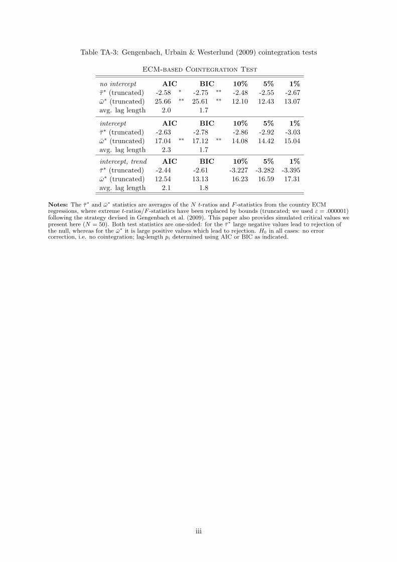
Cointegration tests are commonly carried out as a pre-estimation testing procedure, howeverwe have delayed these until after estimation since we hypothesise that unobservable TFP formspart of the cointegrating vector. Employing our first stage estimate µ•,vat we carried out acointegration testing procedure based on the error correction model representation, first intro-duced by Westerlund (2007) and refined by Gengenbach, Urbain and Westerlund (2009). Thisanalysis (for results see Technical Appendix) implies that there are good grounds to suggestthat value-added per worker, capital per worker and our estimate for TFP are heterogeneouslycointegrated.

We also investigated parameter heterogeneity across countries using a number of formal testingprocedures (results available on request). Taken together these results give a strong indicationthat parameter homogeneity is rejected in our empirical setup. Systematic differences in thetest statistics for levels and first difference specifications indicate that nonstationarity may drivesome of these results. Nevertheless, even if heterogeneity were not very significant in qualitativeterms, our contrasting of pooled and country regression results has shown that it neverthelessmatters greatly for empirical analysis in the presence of nonstationary variables.

In the analysis of empirical production functions the issue of variable endogeneity is typicallyof great concern, requiring means and ways to instrument for inputs. We therefore adoptedthe empirical approach by Pedroni (2000, 2007) and estimated country regressions by Fully-Modified OLS, whereupon parameter estimates are averaged across countries (Group-MeanFMOLS). Provided the variables are nonstationary and cointegrated the individual FMOLSestimates are super-consistent and thus robust to the influence of variable endogeneity andother misspecifications (Pedroni, 2007). Our results (see Technical Appendix) show that thestandard Pedroni (2000) approach yields insignificant capital estimates, whereas augmentation

13

with the common dynamic process yields statistically significant estimates very close to thosearising from our previous AMG regressions. Once we include µ•,vat we thus obtain the sameempirical results in the Group-Mean Fully-Modified OLS and Mean Group OLS approaches.Alternative CCE-type specifications similarly mirror the results in Table 2; furthermore, ouranalysis is robust to a restriction of the sample to countries for which value-added and capitalstock per worker ‘pass’ two (non)stationarity tests (the sample almost halves) and are thus notdriven by sample selection. We take these results as a vindication of our previous findings.

5.7 Discussion of the main empirical results

We investigated the changing parameter estimates across a number of empirical specificationsand estimators. Our pooled estimators in levels are suggested to be severely biased, given thediagnostic tests and the fact that their capital coefficients range from .6 to .8, far in excess ofthe macro evidence of around 1/3. This bias may arise from the misspecification of homogeneityand/or the failure to account for unobserved common factors appropriately. The fact that CCEPyields very similar results to POLS and FE suggests that interplay of parameter heterogeneityand variable stationarity plays an important role. The first difference estimator (FD-OLS) incontrast has sound diagnostics and yields sensible parameter coefficients.

The heterogeneous parameter estimators yield uniformly lower capital coefficients, more inline with the aggregate economy factor income share data. Across levels and first difference,gross-output and value-added specifications (former available on request) there seems to bea consistent pattern whereby the standard heterogeneous MG estimator obtains qualitativelydifferent results from the augmented estimators (AMG, CMG). Diagnostic tests cannot differ-entiate between these two groups of estimators, however we can argue that the MG estimatoris likely to be biased: firstly, it uses an overly simplistic representation for TFP evolution (lin-ear trend) which requires stationarity; secondly, it is argued to suffer from the identificationproblem introduced above.

Turning to the augmented estimators, we suggest that the combination of a common dynamicprocess and a linear country trend is confirmed by the data: a considerable number of countrytrends are statistically significant, while in the models which include µ•t as additional regressorits cross-country average coefficient is close to unity. The CMG estimator provides resultsbroadly in line with those for the AMG, with the latter on the whole more consistent acrossspecifications. The comparison between the country regression results presented above and theresults for ‘demeaned’ variables (available on request) indicate that the unobserved commonfactors exert differential impact across countries, thus meriting the adoption of approacheswhich allow for heterogeneous factor loadings (and thus TFP).

6 TFP in a heterogeneous parameter world

For many applications the estimation of production functions is just the first step in an empir-ical analysis that concentrates on the magnitudes and determinants of TFP — at times TFPis almost treated as if it were an observable variable. In our analysis we have thus far fo-cused on the magnitudes and robustness of the technology parameter estimates across differentproduction function specifications. We now want to provide some estimates for TFP and itsevolution, highlighting some conceptual difficulties arising in the process. From the preferredcountry regressions we can obtain estimates for the intercept, technology parameters, idiosyn-cratic and common trend coefficients or the parameters on the cross-section averages for AMG

14

and CMG specification respectively. One may be tempted to view the coefficients on the inter-cepts as TFP level estimates, just like in the pooled fixed effects case. However, once we allowfor heterogeneity in the slope coefficients, the interpretation of the intercept as an estimate forbase-year TFP level is no longer valid. In order to illustrate our case, we employ a simple linearrelationship between value-added and capital where the contribution of TFP growth has alreadybeen accounted for.

Figure 2: Regression intercepts and TFP level estimates

Korea's log(K/L) in 1970Malaysia's

log(K/L)

in 1970

Malaysia

South Korea

8.5

9

9.5

10

10.5

11

9 10 11 12

Capital stock per worker (in logs)

Belgium

Belgium's

log(K/L) in 1970

France

France's log(K/L) in 197010.2

10.4

10.6

10.8

11.4 11.8 12.2 12.6

Capital stock per worker (in logs)

15

In Figure 2 we provide scatter plots for ‘adjusted’ log value-added per worker (y-axis) againstlog capital per worker (x-axis) as well as a fitted regression line for these observations in eachof the following four countries: in the upper panel France (circles) and Belgium (triangles), inthe lower panel South Korea (circles) and Malaysia (triangles). The ‘adjustment’ is based onthe country-specific estimates from the AMG regression (Table 2, Panel (A), column [3]): wecompute

yadjit = yit − cit− diµ•t (6)

where ci and di are the country-specific estimates for the linear trend term and the commondynamic process respectively. We then plot this variable against log capital per worker for eachcountry separately. This procedure in essence provides a two-dimensional visual equivalent ofthe estimates for the capital coefficient (slope) and the TFP level (intercept) in the augmentedcountry regression. The upper panel of Figure 2 shows two countries (France, Belgium) withvirtually identical capital coefficient estimates (slopes). The in-sample fitted regression line isplotted as a solid line, the out-of-sample extrapolation toward the y-axis is plotted in dashes.The country-estimates for the intercepts can be interpreted as TFP levels, since these countrieshave very similar capital coefficient estimates (bFRA ≈ bBEL). In this case, the graph representsthe linear model yadjit = ai + b log(K/L)it, where ai possesses the ceteris paribus property.In contrast, the lower panel shows two countries (Malaysia, South Korea) which exhibit verydifferent capital coefficient estimates. In this case ai cannot be interpreted as possessing theceteris paribus quality since bMY S 6= bKOR: ceteris non paribus! In the graph we can see thatMalaysia has a considerably higher intercept term than South Korea, even though the latter’sobservations lie above those of the former at any given point in time. This illustrates that oncetechnology parameters in the production function differ across countries the regression interceptcan no longer be interpreted as a TFP-level estimate.

We can suggest an alternative measure for TFP-level which is robust to parameter heterogeneity.Referring back to the scatter plots in Figure 2, we marked the base-year level of log capital perworker by vertical lines for each of the four countries. We suggest to use the locus where thesolid (in-sample) regression line hits the vertical base-year capital stock level as an indicator ofTFP-level in the base year. These adjusted base-year and final-year TFP-levels are thus

ai + bi log(K/L)0,i and ai + bi log(K/L)0,i + ciτ + diµ•τ (7)

respectively, where log(K/L)0,i is the country-specific base-year value for capital per worker(in logs), τ is the total period for which country i is in the sample and µ•τ is the accumulatedcommon TFP growth for this period τ with the country-specific parameter di — it is easy tosee that the intercept-problem discussed above only has bearings on TFP-level estimates. Asimilar formula applies for the CMG estimator.

Focusing exclusively on the TFP-levels in the base-year, Table 3 presents the rank (by magni-tude) for adjusted TFP levels derived from the AMG and CMG estimators. We further show thecountry ranking based on a pooled fixed effects estimation, such as that presented in Table 2,column [2]. As can be seen in the right half of the table, the rankings differ considerably be-tween the AMG or CMG results on the one hand and standard fixed effects results on the other(median absolute rank difference (MARD): 10, respectively), but not between the results forAMG and CMG (MARD: 1).

16

Table 3: Country rankings by TFP-level

Comparison of Country Ranking across Estimators

Country Rank Absolute Rank Difference[1] [2] [3] abs([2]-[1]) abs([3]-[1]) abs([3]-[2])

Country FE AMG† CMG‡ AMG-FE CMG-FE CMG-AMGAUS 12 14 13 2 1 1AUT 22 10 10 12 12 0BEL 24 12 12 12 12 0BGD 34 45 45 11 11 0BOL 4 29 23 25 19 6BRB 33 32 32 1 1 0CAN 6 5 4 1 2 1CHL 3 21 19 18 16 2COL 11 31 31 20 20 0CYP 20 28 29 8 9 1ECU 41 34 36 7 5 2EGY 48 44 44 4 4 0ESP 5 15 16 10 11 1FIN 14 7 6 7 8 1FJI 43 35 34 8 9 1FRA 18 8 7 10 11 1GBR 19 13 14 6 5 1GTM 17 30 30 13 13 0HUN 45 41 42 4 3 1IDN 44 47 48 3 4 1IND 46 48 47 2 1 1IRL 2 17 20 15 18 3IRN 23 23 24 0 1 1ISR 21 2 9 19 12 7ITA 15 4 3 11 12 1KOR 13 25 27 12 14 2LKA 31 46 46 15 15 0LUX 39 6 5 33 34 1MAR 32 42 39 10 7 3MEX 9 19 17 10 8 2MLT 8 38 38 30 30 0MYS 35 39 40 4 5 1NLD 27 9 8 18 19 1NOR 25 11 11 14 14 0NZL 29 16 15 13 14 1PAN 37 22 22 15 15 0PHL 30 37 35 7 5 2POL 47 40 41 7 6 1PRT 36 24 26 12 10 2SEN 38 27 28 11 10 1SGP 10 26 25 16 15 1SWE 16 3 2 13 14 1SWZ 40 43 43 3 3 0TUN 42 36 37 6 5 1TUR 7 18 18 11 11 0USA 1 1 1 0 0 0VEN 28 20 21 8 7 1ZWE 26 33 33 7 7 0

Median 10.3 10.1 1.0

Notes: The table provides the respective TFP level ranking (by magnitude) for each country derived from thethree regression models, as well as the absolute rank differences between them. Country codes are detailed inTable A-II in the Appendix. † AMG refers to the Augmented Mean Group estimator, Table 2, upper panel,column [3]. ‡ CMG refers to the Mean Group version of the Pesaran (2006) CCE estimator, ibid. column [4].The TFP-level adjustment is detailed in Section 6.

17

We present adjusted TFP base-year and final-year levels for these AMG and CMG models inFigure 3.12 The countries in both charts are arranged in order of magnitude of their final-yearadjusted TFP levels in the AMG(ii) model, for which results are shown in the left bar-chart.With exception of a small number of countries (e.g. MLT — Malta, SGP — Singapore) thegeneral ordering of countries by final-year TFP levels is very similar in the two specifications:countries such as Finland, Canada, the United States or Ireland can be found toward the topof the ranking, with Bangladesh, India, Sri Lanka and Poland closer to the bottom.

Figure 3: TFP levels — adjusted from AMG and CMG estimates∗

AMG(ii) CCE(i)

7.0 8.0 9.0 10.0 11.0 12.0

BGD

IND

LKA

POL

TUN

HUN

IDN

FJI

EGY

MAR

PHL

SWZ

GTM

ZWE

SEN

PAN

ECU

BOL

COL

MYS

PRT

CYP

KOR

CHL

MEX

IRN

VEN

TUR

NZL

ESP

BRB

SGP

ISR

NLD

AUS

AUT

GBR

NOR

SWE

BEL

LUX

ITA

FRA

IRL

CAN

USA

FIN

MLT

Final year TFP level (adjusted) Base-year TFP level (adjusted)

7.0 8.0 9.0 10.0 11.0 12.0

BGD

IND

LKA

POL

TUN

HUN

IDN

FJI

EGY

MAR

PHL

SWZ

GTM

ZWE

SEN

PAN

ECU

BOL

COL

MYS

PRT

CYP

KOR

CHL

MEX

IRN

VEN

TUR

NZL

ESP

BRB

SGP

ISR

NLD

AUS

AUT

GBR

NOR

SWE

BEL

LUX

ITA

FRA

IRL

CAN

USA

FIN

MLT

Final year TFP level (adjusted) Base-year TFP level (adjusted)

Notes: Models with CRS imposed. ∗AMG(ii) has µ•t included as additional regressor, CCE(i) refers to thestandard CMG estimator (see Table 2, columns [3] and [4]). Countries are ranked by AMG(ii) final periodTFP-level. Levels adjustment as described in the main text.

12Note that in our sample base- and final-year differ across countries (see Table A-II in the Appendix).

18

7 Concluding remarks

In this paper we investigated how technology differences in manufacturing across countries canbe empirically modelled. We adopted an encompassing framework which allows for the possibil-ity that the impact of observable and unobservable inputs on output differs across countries, aswell as for nonstationary evolution of these processes. We employed empirical estimators whichallow for a globally common, unobserved factor (or factors) interpreted either as common TFPor an average of country-specific TFP evolution. While in the CMG this common dynamicprocess is only implicit, the AMG approach uses an explicit estimate for this process in theaugmentation of country-regressions.

Our empirical framework allowed us to model a number of characteristics which are likely tobe prevalent in manufacturing data from a diverse sample of countries: firstly, we allowed fortechnology heterogeneity across countries. Empirical results are confirmed by formal testingprocedures to suggest that technology parameters in manufacturing production indeed differacross countries. This result supports earlier findings by Durlauf (2001) and Pedroni (2007)using aggregate economy data: if production technology differs in cross-country manufacturing,aggregate economy technology is unlikely to be homogeneous. The result of production tech-nology heterogeneity across countries has immediate implications for standard TFP analysis:it leads to the breakdown of the interpretation of regression intercepts as TFP-level estimates.We therefore introduced a new procedure to compute ‘adjusted’ TFP-level estimates, whichis robust to parameter heterogeneity and can thus be compared across countries and betweenpooled and heterogeneous parameter models.13 Further analysis highlighted the significantdifferences between ‘adjusted’ TFP-level estimates derived from our preferred heterogeneousparameter estimators on the one hand and the standard pooled fixed effects estimator on theother. The finding of cross-country technology heterogeneity thus questions the validity ofstandard development accounting practices to impose common coefficients on capital stock toextract country-specific measures of TFP, a recognised shortcoming in this literature (Caselli,2008).

Secondly, we allowed for unobserved common factors to drive output, but with differentialimpact across countries, thus inducing cross-section dependence. These common factors arevisualised by our common dynamic process, which follows patterns over the 1970-2002 sampleperiod that match historical events. The interpretation of this common dynamic process µ•twould be that for the manufacturing sector similar factors drive production in all countries,albeit to a different extent. This is equivalent to suggesting that the ‘global tide’ of innovationcan ‘lift all boats’, and that technology transfer from developed to developing countries ispossible but dependent on the country’s production technology and absorptive capacity, amongother things.

Thirdly, our empirical setup allows for a type of endogeneity which is arguably very intuitive,namely that some of the unobservables driving output are also driving the evolution of inputs.This leads to an identification problem, whereby standard panel estimators cannot identify theparameters on the observable inputs as distinct from the impact of unobservables. AdditionalMonte Carlo simulations (Bond and Eberhardt, 2009) have highlighted the ability of the Pesaran(2006) CCE estimators and the AMG approach to deal with this problem successfully. Further-more, additional analysis confirms that the empirical results are robust to the use of a paneltime-series econometric approach. The Pedroni (2000) Group-Mean FMOLS approach suggeststhat failure to account for unobserved common factors when analysing cross-country manufac-turing production leads to the breakdown of the empirical estimates, whereas the inclusion ofthe common dynamic process yields results very close to those from the AMG and CMG. Stan-

13Issues of estimate precision could be addressed using bootstrapping to construct standard errors.

19

dard practices to deal with endogeneity (Arellano and Bond, 1991; Blundell and Bond, 1998)are only appropriate in a stationary framework with homogeneous technology (Pesaran andSmith, 1995). This aside many researchers have expressed concerns over instrument validityin macro panel data (e.g. Clemens and Bazzi, 2009). Adopting a nonstationary panel econo-metric approach that accounts for cross-section dependence in our view is a sound empiricalalternative to address both these concerns and should be applied more widely to cross-countryproductivity-analysis.

References

Abramowitz, Moses (1956). “Resource and output trend in the United States since 1870.”American Economic Review, Vol. 46(2): 5–23.

Arellano, Manuel and Bond, Stephen R. (1991). “Some tests of specification for panel data.”Review of Economic Studies, Vol. 58(2): 277–297.

Azariadis, Costas and Drazen, Allan (1990). “Threshold Externalities in Economic Develop-ment.” Quarterly Journal of Economics, Vol. 105(2): 501–26.

Bai, Jushan (2009a). “Likelihood approach to small T dynamic panel models with interactiveeffects.” Unpublished working paper, June 2009.

Bai, Jushan (2009b). “Panel Data Models with Interactive Fixed Effects.” Econometrica,Vol. 77(4): 1229–1279.

Bai, Jushan and Ng, Serena (2004). “A PANIC attack on unit roots and cointegration.” Econo-metrica, Vol. 72(4): 191–221.

Bai, Jushan and Ng, Serena (2008). “Large Dimensional Factor Analysis.” Foundations andTrends in Econometrics, Vol. 3(2): 89–163.

Banerjee, Abhijit V. and Newman, Andrew F. (1993). “Occupational Choice and the Processof Development.” Journal of Political Economy, Vol. 101(2): 274–98.

Barro, Robert J. (1991). “Economic growth in a cross-section of countries.” Quarterly Journalof Economics, Vol. 106(2): 407–443.

Bernard, Andrew B. and Jones, Charles I. (1996a). “Comparing Apples to Oranges: Produc-tivity Convergence and Measurement across Industries and Countries.” American EconomicReview, Vol. 86(5): 1216–38.

Bernard, Andrew B. and Jones, Charles I. (1996b). “Productivity across Industries and Coun-tries: Time Series Theory and Evidence.” The Review of Economics and Statistics, Vol. 78(1):135–46.

Blundell, Richard and Bond, Stephen R. (1998). “Initial conditions and moment restrictions indynamic panel data models.” Journal of Econometrics, Vol. 87(1): 115–143.

Bond, Stephen R. and Eberhardt, Markus (2009). “Cross-section dependence in nonstationarypanel models: a novel estimator.” Paper presented at the Nordic Econometrics Meeting inLund, Sweden, October 29-31.

Bond, Stephen R., Hoeffler, Anke and Temple, Jonathan (2001). “GMM Estimation of EmpiricalGrowth Models.”

Bond, Stephen R., Leblebicioglu, Asli and Schiantarelli, Fabio (2007). “Capital Accumulationand Growth: A New Look at the Empirical Evidence.” Unpublished working paper.

20

Bond, Stephen R., Leblebicioglu, Asli and Schiantarelli, Fabio (2010). “Capital Accumulationand Growth: A New Look at the Empirical Evidence.” Journal of Applied Econometrics.Forthcoming.

Canning, David and Pedroni, Peter (2008). “Infrastructure, Long-Run Economic Growth AndCausality Tests For Cointegrated Panels.” Manchester School, Vol. 76(5): 504–527.

Caselli, Francesco (2008). “Level Accounting.” In: Steven N. Durlauf and Lawrence E. Blume(Editors), “The New Palgrave Dictionary of Economics Online,” (Palgrave Macmillan), sec-ond edition.

Caselli, Francesco, Esquivel, Gerardo and Lefort, Fernando (1996). “Reopening the ConvergenceDebate: A New Look at Cross-Country Growth Empirics.” Journal of Economic Growth,Vol. 1(3): 363–89.

Chudik, Alexander, Pesaran, M. Hashem and Tosetti, Elisa (2010). “Weak and Strong CrossSection Dependence and Estimation of Large Panels.” Econometrics Journal. Forthcoming.

Clemens, Michael and Bazzi, Samuel (2009). “Blunt Instruments: On Establishing the Causesof Economic Growth.” Center for Global Development Working Papers #171.

Coakley, Jerry, Fuertes, Ana-Maria and Smith, Ron P. (2001). “Small sample properties ofpanel time-series estimators with I(1) errors.” Unpublished working paper.

Coakley, Jerry, Fuertes, Ana-Maria and Smith, Ron P. (2006). “Unobserved heterogeneity inpanel time series models.” Computational Statistics & Data Analysis, Vol. 50(9): 2361–2380.

Coe, David T. and Helpman, Elhanan (1995). “International R&D spillovers.” European Eco-nomic Review, Vol. 39(5): 859–887.

Coe, David T., Helpman, Elhanan and Hoffmaister, Alexander W. (1997). “North-South R&DSpillovers.” Economic Journal, Vol. 107(440): 134–49.

Costantini, Mauro and Destefanis, Sergio (2009). “Cointegration analysis for cross-sectionallydependent panels: The case of regional production functions.” Economic Modelling,Vol. 26(2): 320–327.

Durlauf, Steven N. (1993). “Nonergodic Economic Growth.” Review of Economic Studies,Vol. 60(2): 349–66.

Durlauf, Steven N. (2001). “Manifesto for a growth econometrics.” Journal of Econometrics,Vol. 100(1): 65–69.

Durlauf, Steven N., Johnson, Paul A. and Temple, Jonathan R.W. (2005). “Growth Economet-rics.” In: Philippe Aghion and Steven Durlauf (Editors), “Handbook of Economic Growth,”Vol. 1 of Handbook of Economic Growth, chapter 8 (Elsevier), pp. 555–677.

Durlauf, Steven N., Kourtellos, Andros and Minkin, Artur (2001). “The local Solow growthmodel.” European Economic Review, Vol. 45(4-6): 928–940.

Durlauf, Steven N. and Quah, Danny T. (1999). “The new empirics of economic growth.” In:J. B. Taylor and M. Woodford (Editors), “Handbook of Macroeconomics,” Vol. 1 of Handbookof Macroeconomics, chapter 4 (Elsevier), pp. 235–308.

Eberhardt, Markus and Teal, Francis (2010). “Econometrics for Grumblers: A New Look at theLiterature on Cross-Country Growth Empirics.” Journal of Economic Surveys. Forthcoming.

Engelbrecht, Hans-Jurgen (2002). “Human Capital and International Knowledge Spilloversin TFP Growth of a Sample of Developing Countries: An Exploration of Alternative Ap-proaches.” Applied Economics, Vol. 34(7): 831–41.

21

Fleisher, Belton, Li, Haizheng and Zhao, Min Qiang (2010). “Human capital, economic growth,and regional inequality in China.” Journal of Development Economics, Vol. 92(2): 215–231.

Funk, Mark and Strauss, Jack (2003). “Panel tests of stochastic convergence: TFP transmissionwithin manufacturing industries.” Economics Letters, Vol. 78(3): 365–371.

Gengenbach, Christian, Urbain, Jean-Pierre and Westerlund, Joakim (2009). “Panel ErrorCorrection Testing with Global Stochastic Trends.” Unpublished working paper, Maastricht:METEOR.

Gomme, Paul and Rupert, Peter (2004). “Measuring Labor’s Share of Income.” Federal ReserveBank of Cleveland Policy Discussion Paper, November.

Granger, Clive W. J. (1997). “On Modelling the Long Run in Applied Economics.” EconomicJournal, Vol. 107(440): 169–77.

Harrigan, James (1999). “Estimation of cross-country differences in industry production func-tions.” Journal of International Economics, Vol. 47(2): 267–293.

Hendry, David (1995). Dynamic Econometrics. Advanced Texts in Econometrics (OxfordUniversity Press).

Hultberg, Patrik T., Nadiri, M. Ishaq and Sickles, Robin C. (2004). “Cross-country catch-up inthe manufacturing sector: Impacts of heterogeneity on convergence and technology adoption.”Empirical Economics, Vol. 29(4): 753–768.

Im, Kyung So, Pesaran, M. Hashem and Shin, Yongcheol (1997). “Testing for unit roots inheterogeneous panels.” Discussion Paper, University of Cambridge.

Islam, Nazrul (2003). “What have We Learnt from the Convergence Debate?” Journal ofEconomic Surveys, Vol. 17(3): 309–362.

Jones, Charles I. (1995). “Time Series Tests of Endogenous Growth Models.” Quarterly Journalof Economics, Vol. 110(2): 495–525.

Kao, Chihwa (1999). “Spurious regression and residual-based tests for cointegration in paneldata.” Journal of Econometrics, Vol. 65(1): 9–15.

Kao, Chihwa, Chiang, Min-Hsien and Chen, Bangtian (1999). “International R&D spillovers:An application of estimation and inference in panel cointegration.” Oxford Bulletin of Eco-nomics and Statistics, Vol. 61(Special Issue): 691–709.

Kapetanios, George, Pesaran, M. Hashem and Yamagata, Takashi (2010). “Panels with Non-stationary Multifactor Error Structures.” Journal of Econometrics. Forthcoming.

Klenow, Peter J. and Rodriguez-Clare, Andres (1997). “Economic growth: A review essay.”Journal of Monetary Economics, Vol. 40(3): 597–617.

Larson, Donald F., Butzer, Rita, Mundlak, Yair and Crego, Al (2000). “A cross-countrydatabase for sector investment and capital.” World Bank Economic Review, Vol. 14(2):371–391.

Lee, Kevin, Pesaran, M. Hashem and Smith, Ron P. (1997). “Growth and Convergencein a Multi-country Empirical Stochastic Solow Model.” Journal of Applied Econometrics,Vol. 12(4): 357–92.

Levinsohn, James and Petrin, Amil (2003). “Estimating Production Functions Using Inputs toControl for Unobservables.” Review of Economic Studies, Vol. 70(2): 317–341.

22

Maddala, G. S. and Wu, Shaowen (1999). “A comparative study of unit root tests with paneldata and a new simple test.” Oxford Bulletin of Economics and Statistics, Vol. 61(SpecialIssue): 631–652.

Malley, Jim, Muscatelli, Anton and Woitek, Ulrich (2003). “Some new international comparisonsof productivity performance at the sectoral level.” Journal of the Royal Statistical Society:Series A, Vol. 166(1): 85–104.

Mankiw, N. Gregory, Romer, David and Weil, David N. (1992). “A Contribution to the Empiricsof Economic Growth.” Quarterly Journal of Economics, Vol. 107(2): 407–437.

Martin, Will and Mitra, Devashish (2002). “Productivity Growth and Convergence in Agri-culture versus Manufacturing.” Economic Development and Cultural Change, Vol. 49(2):403–422.

Moscone, Francesco and Tosetti, Elisa (2009). “A Review And Comparison Of Tests Of Cross-Section Independence In Panels.” Journal of Economic Surveys, Vol. 23(3): 528–561.

Murphy, Kevin M., Shleifer, Andrei and Vishny, Robert W. (1989). “Industrialization and theBig Push.” Journal of Political Economy, Vol. 97(5): 1003–26.

Nelson, Charles R. and Plosser, Charles R. (1982). “Trends and random walks in macroeconomictime series: some evidence and implications.” Journal of Monetary Economics, Vol. 10(2):139–162.

Pagan, Adrian (1984). “Econometric Issues in the Analysis of Regressions with GeneratedRegressors.” International Economic Review, Vol. 25(1): 221–247.

Pedroni, Peter (1999). “Critical values for cointegration tests in heterogeneous panels withmultiple regressors.” Oxford Bulletin of Economics and Statistics, Vol. 61(Special Issue):653–670.

Pedroni, Peter (2000). “Fully modified OLS for heterogeneous cointegrated panels.” In: Badi H.Baltagi (Editor), “Nonstationary panels, cointegration in panels and dynamic panels,” (Am-sterdam: Elsevier).

Pedroni, Peter (2001). “Purchasing Power Parity Tests In Cointegrated Panels.” The Reviewof Economics and Statistics, Vol. 83(4): 727–731.

Pedroni, Peter (2007). “Social capital, barriers to production and capital shares: implicationsfor the importance of parameter heterogeneity from a nonstationary panel approach.” Journalof Applied Econometrics, Vol. 22(2): 429–451.

Pesaran, M. Hashem (2006). “Estimation and inference in large heterogeneous panels with amultifactor error structure.” Econometrica, Vol. 74(4): 967–1012.

Pesaran, M. Hashem (2007). “A simple panel unit root test in the presence of cross-sectiondependence.” Journal of Applied Econometrics, Vol. 22(2): 265–312.

Pesaran, M. Hashem and Smith, Ron P. (1995). “Estimating long-run relationships from dy-namic heterogeneous panels.” Journal of Econometrics, Vol. 68(1): 79–113.

Pesaran, M. Hashem and Tosetti, Elisa (2010). “Large Panels with Common Factors and SpatialCorrelations.” Cambridge University, unpublished working paper, May.

Phillips, Peter C. B. and Moon, Hyungsik Roger (1999). “Linear regression limit theory fornonstationary panel data.” Econometrica, Vol. 67(5): 1057–1112.

Quah, Danny (1997). “Empirics for Growth and Distribution: Stratification, Polarization, andConvergence Clubs.” Journal of Economic Growth, Vol. 2(1): 27–59.

23

Ranis, Gustav and Fei, John (1988). The State of Development Economics, chapter DevelopmentEconomics: what next? (Oxford: Blackwell).

Rapach, David E. (2002). “Are Real GDP Levels Nonstationary? Evidence from Panel DataTests.” Southern Economic Journal, Vol. 68(3): 473–495.

Sarafidis, Vasilis and Wansbeek, Tom (2010). “Cross-sectional Dependence in Panel Data Anal-ysis.” Unpublished working paper, MPRA Paper 20815.

Smith, Ron P. and Fuertes, Ana-Maria (2007). “Panel Time Series.” Centre for MicrodataMethods and Practice (cemmap) mimeo, April 2007.

Smith, Ron P. and Tasiran, Ali (2010). “Random coefficient models of arms imports.” EconomicModelling : forthcoming.

Swamy, P. A. V. B. (1970). “Efficient Inference in a Random Coefficient Regression Model.”Econometrica, Vol. 38(2): 311–23.

Temple, Jonathan (1999). “The New Growth Evidence.” Journal of Economic Literature,Vol. 37(1): 112–156.

UN (2005). “UN Common Statistics 2005.” Online database, New York: UN, United Nations.

UNIDO (2004). “UNIDO Industrial Statistics 2004.” Online database, Vienna: UNIDO, UnitedNations Industrial Development Organisation.

Westerlund, Joakim (2007). “Testing for Error Correction in Panel Data.” Oxford Bulletin ofEconomics and Statistics, Vol. 69(6): 709–748.

24

Appendix: Data construction and descriptives

Data for output, value-added, material inputs and investment in manufacturing, all in currentlocal currency units (LCU), are taken from the UNIDO Industrial Statistics 2004 (UNIDO,2004), where material inputs were derived as the difference between output and value-added.The labour data series is taken from the same source, which covers 1963-2002. The capitalstocks are calculated from investment data which has been transformed into constant US$ (seebelow) following the ‘perpetual inventory’ method discussed in Klenow and Rodriguez-Clare(1997).

In order to make data in monetary values internationally comparable, it is necessary to transformall values into a common unit of analysis. We follow the transformations suggested by Martinand Mitra (2002) and derive all values in 1990 US$,a using current LCU and exchange rate datafrom UNIDO, and GDP deflators from the UN Common Statistics database (UN, 2005), forwhich data are available from 1970-2003. Since our model is for a small open economy, we preferusing a single market exchange rates (LCU-US$ exchange rate for 1990) to purchasing-power-parity (PPP) adjusted exchange rates, since the latter are more appropriate when non-tradedservices need to be accounted.

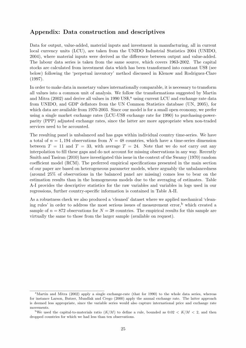
The resulting panel is unbalanced and has gaps within individual country time-series. We havea total of n = 1, 194 observations from N = 48 countries, which have a time-series dimensionbetween T = 11 and T = 33, with average T = 24. Note that we do not carry out anyinterpolation to fill these gaps and do not account for missing observations in any way. RecentlySmith and Tasiran (2010) have investigated this issue in the context of the Swamy (1970) randomcoefficient model (RCM). The preferred empirical specifications presented in the main sectionof our paper are based on heterogeneous parameter models, where arguably the unbalancedness(around 25% of observations in the balanced panel are missing) comes less to bear on theestimation results than in the homogeneous models due to the averaging of estimates. TableA-I provides the descriptive statistics for the raw variables and variables in logs used in ourregressions, further country-specific information is contained in Table A-II.

As a robustness check we also produced a ‘cleaned’ dataset where we applied mechanical ‘clean-ing rules’ in order to address the most serious issues of measurement error,b which created asample of n = 872 observations for N = 38 countries. The empirical results for this sample arevirtually the same to those from the larger sample (available on request).

aMartin and Mitra (2002) apply a single exchange-rate (that for 1990) to the whole data series, whereasfor instance Larson, Butzer, Mundlak and Crego (2000) apply the annual exchange rate. The latter approachis deemed less appropriate, since the variable series would also capture international price and exchange ratemovements.

bWe used the capital-to-materials ratio (K/M) to define a rule, bounded as 0.02 < K/M < 2, and thendropped countries for which we had less than ten observations.

25

Table A-I: Descriptive statistics

Variables in Level Terms

Variable obs mean median std. dev. min. max.levelsvalue-added 1,194 5.47E+10 9.04E+09 1.78E+11 1.76E+07 1.50E+12labour 1,194 1,469,186 502,214 2,924,524 5,552 1.97E+07capital 1,194 1.32E+11 2.61E+10 3.12E+11 5.78E+07 2.27E+12logsvalue-added 1,194 22.70 22.93 2.15 16.68 28.04labour 1,194 12.92 13.13 1.79 8.62 16.79capital 1,194 23.72 23.98 2.22 17.87 28.45annual growth ratevalue-added 1,128 3.9% 3.5% 12.3% -78.3% 92.7%labour 1,128 1.7% 0.7% 8.1% -38.8% 78.1%capital 1,128 4.1% 3.1% 4.4% -2.4% 47.8%

Variables in per worker terms

Variable obs mean median std. dev. min. max.levelsvalue-added 1,194 76,932 45,865 72,843 2,007 346,064capital 1,194 25,305 17,867 19,385 1,660 91,011logsvalue-added 1,194 9.78 9.79 0.92 7.41 11.42capital 1,194 10.80 10.73 1.00 7.60 12.75annual growth ratevalue-added 1,128 2.2% 2.5% 10.8% -90.3% 74.4%capital 1,128 2.5% 2.5% 7.9% -68.0% 45.4%

Notes: We report the descriptive statistics for value-added, labour and capital stock for N = 48 countries andn = 1, 194 (n = 1, 128) observations in the levels (growth) specification. Monetary values are in real US$ (baseyear 1990). Labour is in number of workers.

26

Table A-II: Sample of countries and number of observations

Sample

Country Code levels FD t = 1 t = T I(1)∗

Australia AUS 20 17 1970 1993 XAustria AUT 30 28 1970 2000 XBelgium BEL 28 27 1970 1997 XBangladesh BGD 14 12 1970 1992 XBolivia BOL 11 10 1987 1997Barbados BRB 26 25 1970 1995Canada CAN 21 20 1970 1990 XChile CHL 25 24 1974 1998 XColombia COL 30 29 1970 1999 XCyprus CYP 33 32 1970 2002 XEcuador ECU 30 29 1970 1999Egypt EGY 26 25 1970 1995Spain ESP 26 25 1970 1995Finland FIN 28 26 1970 2000 XFiji FJI 25 24 1970 1994 XFrance FRA 26 25 1970 1995United Kingdom GBR 23 22 1970 1992 XGuatemala GTM 16 15 1973 1988 XHungary HUN 26 25 1970 1995Indonesia IDN 26 25 1970 1995 XIndia IND 32 31 1970 2001Ireland IRL 22 21 1970 1991Iran IRN 24 22 1970 2001Israel ISR 13 12 1989 2001Italy ITA 31 30 1970 2000Korea KOR 32 31 1970 2001Sri Lanka LKA 20 17 1970 2000 XLuxembourg LUX 23 22 1970 1992 XMorocco MAR 17 16 1985 2001 XMexico MEX 16 14 1984 2000 XMalta MLT 32 31 1970 2001 XMalaysia MYS 28 25 1970 2001Netherlands NLD 24 23 1970 1993 XNorway NOR 32 31 1970 2001 XNew Zealand NZL 21 20 1970 1990Panama PAN 30 28 1970 2000Philippines PHL 26 25 1970 1995Poland POL 31 30 1970 2000 XPortugal PRT 31 30 1970 2000 XSenegal SEN 17 14 1970 1990Singapore SGP 33 32 1970 2002 XSweden SWE 18 17 1970 1987 XSwaziland SWZ 24 22 1970 1995Tunisia TUN 21 19 1970 1997Turkey TUR 27 25 1970 1997United States USA 26 25 1970 1995 XVenezuela VEN 26 24 1970 1998 XZimbabwe ZWE 27 26 1970 1996Obs 1,194 1,128 644

Notes: ∗This refers to the sample used in the second set of GM-FMOLS regressions (see Technical Appendix).

27

Technical Appendix

Table TA-1: First generation panel unit root tests

Im, Pesaran & Shin (1997) Panel Unit Root Tests — IPS]

output value-added labour capital materialslags [t-bar] lags [t-bar] lags [t-bar] lags [t-bar] lags [t-bar]

in levels1.42 -1.57 1.96 -1.54 1.48 -1.78 ∗∗ 1.50 -1.92 ∗∗ 1.65 -1.67

in per worker terms1.44 -0.92 1.65 -1.03 1.71 -0.97 1.83 -1.05

Maddala & Wu (1999) Panel Unit Root Tests — MW†

output value-added labour capital materialslags pλ (p) lags pλ (p) lags pλ (p) lags pλ (p) lags pλ (p)

in levels0 129.37 (.01) 0 125.69 (.02) 0 142.42 (.00) 0 274.01 (.00) 0 126.47 (.02)1 126.57 (.02) 1 109.99 (.16) 1 141.35 (.00) 1 67.05 (.99) 1 133.62 (.01)

1.42 69.12 (.98) 1.96 85.44 (.77) 1.48 114.54 (.10) 1.50 55.16 (1.00) 1.65 66.65 (.99)2 114.75 (.09) 2 124.13 (.03) 2 105.34 (.24) 2 80.86 (.87) 2 134.85 (.01)3 74.36 (.95) 3 56.97 (1.00) 3 88.76 (.69) 3 87.84 (.71) 3 108.31 (.18)

in per worker terms0 107.76 (.19) 0 102.23 (.31) 0 54.16 (1.00) 0 102.35 (.31)1 70.70 (.98) 1 84.92 (.78) 1 60.09 (1.00) 1 77.74 (.91)

1.44 30.08 (1.00) 1.65 63.13 (1.00) 1.71 32.32 (1.00) 1.83 32.45 (1.00)2 75.85 (.94) 2 65.26 (.99) 2 34.04 (1.00) 2 77.85 (.91)3 61.41 (1.00) 3 44.65 (1.00) 3 66.85 (.99) 3 87.42 (.72)

in first difference0 924.25 (.00) 0 976.37 (.00) 0 608.63 (.00) 0 248.03 (.00) 0 931.98 (.00)1 500.47 (.00) 1 547.05 (.00) 1 405.04 (.00) 1 214.11 (.00) 1 428.13 (.00)2 320.97 (.00) 2 358.92 (.00) 2 248.07 (.00) 2 154.10 (.00) 2 281.42 (.00)3 322.88 (.00) 3 334.27 (.00) 3 310.84 (.00) 3 169.69 (.00) 3 331.29 (.00)

in first difference of per worker terms0 1007.23 (.00) 0 1061.64 (.00) 0 769.82 (.00) 0 979.89 (.00)1 593.33 (.00) 1 590.67 (.00) 1 439.72 (.00) 1 610.50 (.00)2 348.43 (.00) 2 396.30 (.00) 2 253.49 (.00) 2 301.62 (.00)3 296.79 (.00) 3 285.86 (.00) 3 372.73 (.00) 3 354.89 (.00)

Notes: All variables are in logarithms. ] We report the average of the country-specific ‘ideal’ lag-augmentation(via AIC) and the t-bar statistic, constructed as t-bar = (1/N)

∑i ti (ti are country ADF t-statistics). Under

the H0 of all country series containing a nonstationary process this statistic has a non-standard distribution:the critical values (-1.73 for 5%, -1.69 for 10% significance level — distribution is approximately t) are reportedin Table 2, Panel A of their paper. We indicate the cases where the null is rejected with ∗∗. † We report theMW statistic, constructed as pλ = −2

∑i log(pi) (pi are country ADF statistic p-values) for different

lag-augmentations, including the ‘ideal’ augmentation determined via AIC (levels variables only). Under the H0

of all country series containing a nonstationary process this statistic is distributed χ2(2N). We further reportthe p-values for each of the MW tests.

i

Table TA-2: Second generation panel unit root tests

Pesaran (2007) Panel Unit Root Tests — CIPS]

output value-added labour capital materialslags Z[t-bar] (p) lags Z[t-bar] (p) lags Z[t-bar] (p) lags Z[t-bar] (p) lags Z[t-bar] (p)

in levels0 -1.22 (.11) 0 -1.85 (.03) 0 2.39 (.99) 0 5.11 (1.00) 0 0.29 (.62)1 0.01 (.51) 1 0.06 (.52) 1 1.26 (.90) 1 3.79 (1.00) 1 0.89 (.81)

1.42 1.13 (.87) 1.96 3.54 (1.00) 1.48 3.74 (1.00) 1.50 4.55 (1.00) 1.65 3.68 (1.00)2 2.65 (1.00) 2 2.30 (.99) 2 4.21 (1.00) 2 3.96 (1.00) 2 1.05 (.85)3 7.04 (1.00) 3 3.59 (1.00) 3 4.76 (1.00) 3 7.64 (1.00) 3 4.21 (1.00)

in per worker terms0 -1.08 (.14) 0 -2.55 (.01) 0 1.92 (.97) 0 0.57 (.72)1 2.91 (1.00) 1 -0.73 (.23) 1 1.33 (.91) 1 3.74 (1.00)

1.44 5.98 (1.00) 1.65 3.77 (1.00) 1.71 5.92 (1.00) 1.83 9.62 (1.00)2 5.02 (1.00) 2 2.37 (.99) 2 4.60 (1.00) 2 5.96 (1.00)3 8.73 (1.00) 3 5.48 (1.00) 3 7.34 (1.00) 3 8.08 (1.00)

in first differences0 -17.71 (.00) 0 -19.75 (.00) 0 -15.22 (.00) 0 -6.64 (.00) 0 -18.14 (.00)1 -9.46 (.00) 1 -11.95 (.00) 1 -8.93 (.00) 1 -5.26 (.00) 1 -8.34 (.00)2 -2.00 (.02) 2 -3.65 (.00) 2 -3.14 (.00) 2 -1.20 (.12) 2 -1.59 (.06)3 1.65 (.95) 3 0.67 (.75) 3 0.49 (.69) 3 2.27 (.99) 3 3.16 (1.00)

in first difference of per worker terms0 -19.54 (.00) 0 -20.91 (.00) 0 -15.40 (.00) 0 -18.43 (.00)1 -10.89 (.00) 1 -11.40 (.00) 1 -9.60 (.00) 1 -9.52 (.00)2 -1.95 (.03) 2 -4.21 (.00) 2 -3.37 (.00) 2 -1.83 (.03)3 2.53 (.99) 3 0.11 (.54) 3 0.54 (.71) 3 2.86 (1.00)

Notes: All variables are in logarithms. ] In the third row for each variable in levels we present the CIPS teststatistic for ‘ideal’ lag augmentation of the underlying ADF regression (based on Akaike information criteria);the value for lags reported here is the average across countries.

ii

Table TA-3: Gengenbach, Urbain & Westerlund (2009) cointegration tests

ECM-based Cointegration Test

no intercept AIC BIC 10% 5% 1%τ∗ (truncated) -2.58 ∗ -2.75 ∗∗ -2.48 -2.55 -2.67ω∗ (truncated) 25.66 ∗∗ 25.61 ∗∗ 12.10 12.43 13.07avg. lag length 2.0 1.7

intercept AIC BIC 10% 5% 1%τ∗ (truncated) -2.63 -2.78 -2.86 -2.92 -3.03ω∗ (truncated) 17.04 ∗∗ 17.12 ∗∗ 14.08 14.42 15.04avg. lag length 2.3 1.7

intercept, trend AIC BIC 10% 5% 1%τ∗ (truncated) -2.44 -2.61 -3.227 -3.282 -3.395ω∗ (truncated) 12.54 13.13 16.23 16.59 17.31avg. lag length 2.1 1.8

Notes: The τ∗ and ω∗ statistics are averages of the N t-ratios and F -statistics from the country ECMregressions, where extreme t-ratios/F -statistics have been replaced by bounds (truncated; we used ε = .000001)following the strategy devised in Gengenbach et al. (2009). This paper also provides simulated critical values wepresent here (N = 50). Both test statistics are one-sided: for the τ∗ large negative values lead to rejection ofthe null, whereas for the ω∗ it is large positive values which lead to rejection. H0 in all cases: no errorcorrection, i.e. no cointegration; lag-length pi determined using AIC or BIC as indicated.

iii

Table TA-4: Country regressions using FMOLS

Panel A: Full Sample (N=48)

[1] [2] [3] [4] [5]estimator : FMOLS- MG AMG AMG CMG CMG

dependent variable ly ly-µ•,vat ly ly lylog capital pw 0.1663 0.2659 0.2937 0.5544 0.3042

[1.99] [3.32]∗∗ [3.18]∗∗ [8.05]∗∗ [3.33]∗∗

common process 0.8977[3.49]∗∗

country trends 0.0171 0.0004 0.0014 0.0108[5.50]∗∗ [0.12] [0.29] [2.95]∗∗

intercept -4.6095 6.5985 7.1405 5.6737 -1.6007[1.63] [2.69]∗∗ [1.52] [5.57]∗∗ [0.57]

Panel-t statistics, diagnosticscapital pw 18.29 14.73 15.36 40.59 15.88trends 24.94 18.93 12.71 20.70# of sign. trends (at 10%) 37 25 23 28RMSE .099 .096 .090 .103 .088

Panel B: I(1) Sample (N=26)

[1] [2] [3] [4] [5]estimator : FMOLS- MG AMG AMG CMG CMG

dependent variable ly ly-µ•,vat ly ly lylog capital pw 0.0816 0.2675 0.2784 0.5528 0.2485

[1.27] [4.11]∗∗ [3.08]∗∗ [7.38]∗∗ [3.13]∗∗

common process 0.8034[4.61]∗∗

country trends 0.0179 -0.0012 0.0019 0.0108[5.64]∗∗ [0.40] [0.41] [2.56]∗

intercept -4.9092 6.1012 5.2980 5.3936 -2.3070[1.59] [2.63]∗ [1.50] [4.60]∗∗ [0.76]

Panel-t statistics, diagnosticscapital pw 11.45 10.37 9.97 34.96 10.16trends 23.28 14.63 10.56 17.10# of sign. trends (at 10%) 23 15 15 16RMSE .071 .068 .065 .080 .062

Notes: The results in [1] are for the Pedroni (2000) Group-Mean FMOLS estimator; the results in theremaining columns allow for cross-section dependence using either µ•,vat or cross-section averages in the FMOLScountry regressions. In all cases the estimates presented are the unweighted means of the FMOLS countryestimates. Panel B uses observations from only those countries for which variables were determined to benonstationary (via ADF and KPSS testing).

iv