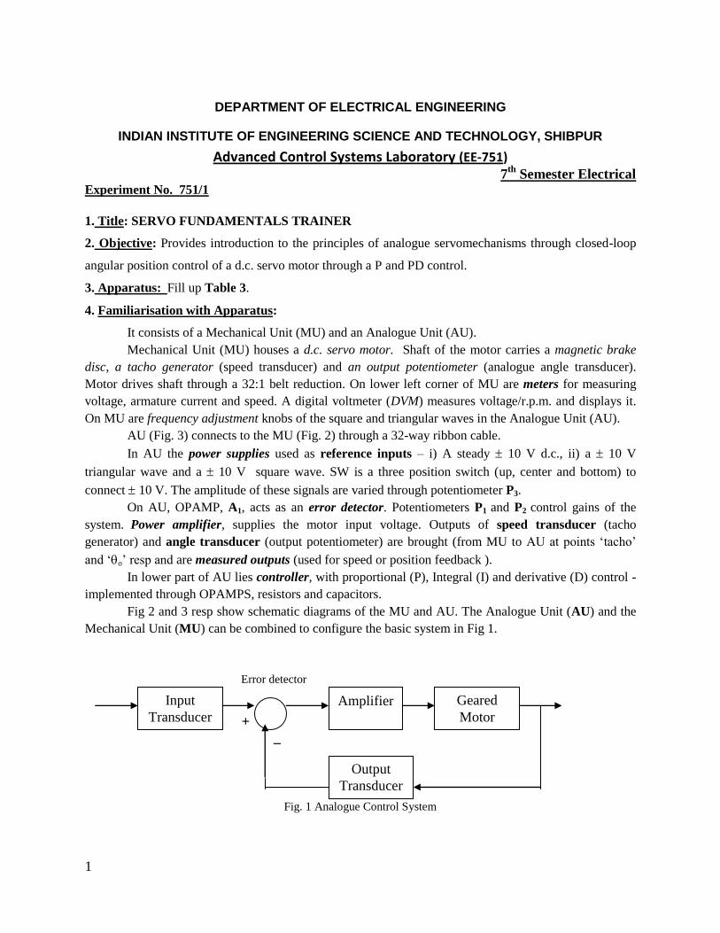
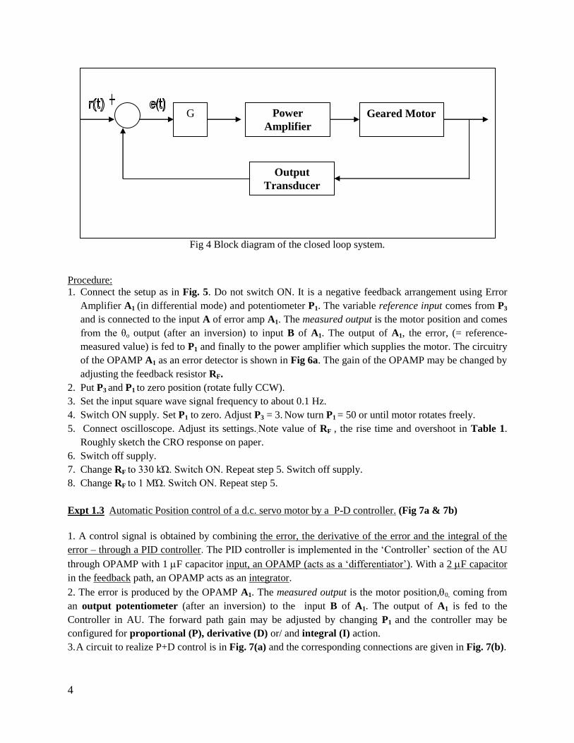
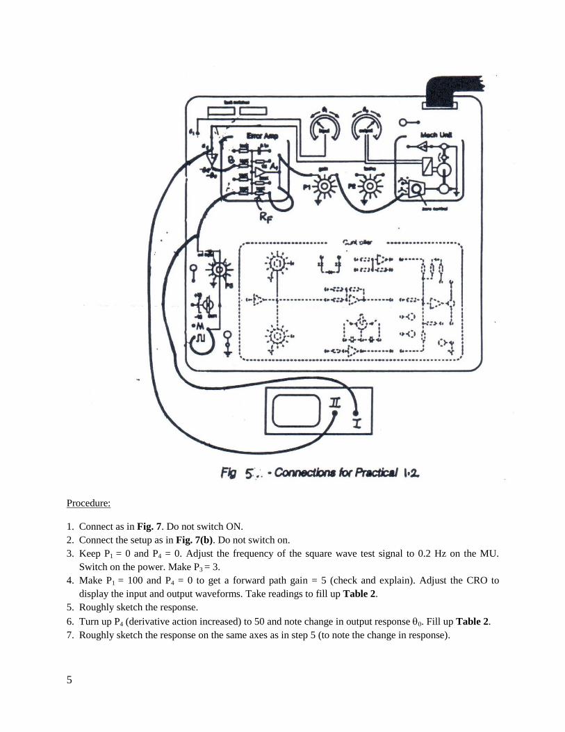
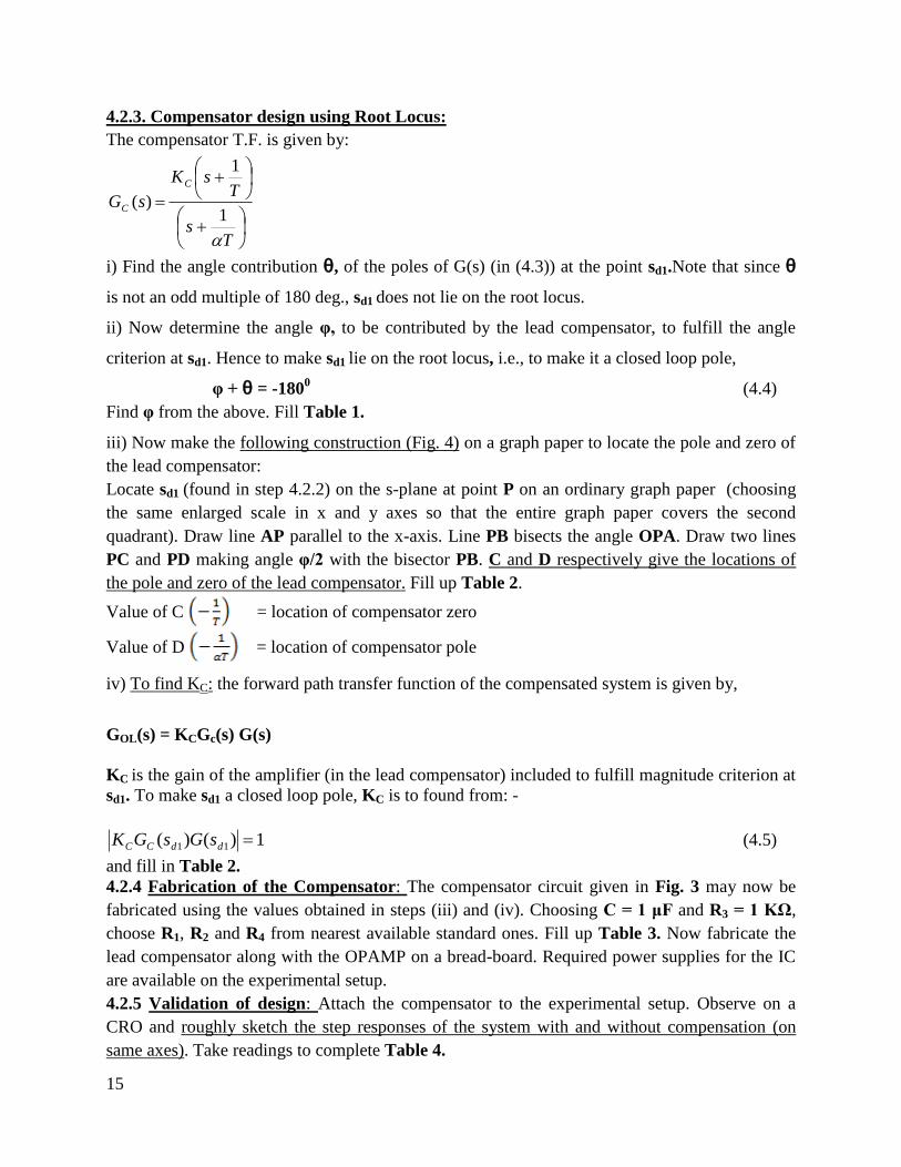
1
DEPARTMENT OF ELECTRICAL ENGINEERING
INDIAN INSTITUTE OF ENGINEERING SCIENCE AND TECHNOLOGY, SHIBPUR
Advanced Control Systems Laboratory (EE-751) 7
th Semester Electrical
Experiment No. 751/1
1. Title: SERVO FUNDAMENTALS TRAINER
2. Objective: Provides introduction to the principles of analogue servomechanisms through closed-loop
angular position control of a d.c. servo motor through a P and PD control.
3. Apparatus: Fill up Table 3.
4. Familiarisation with Apparatus:
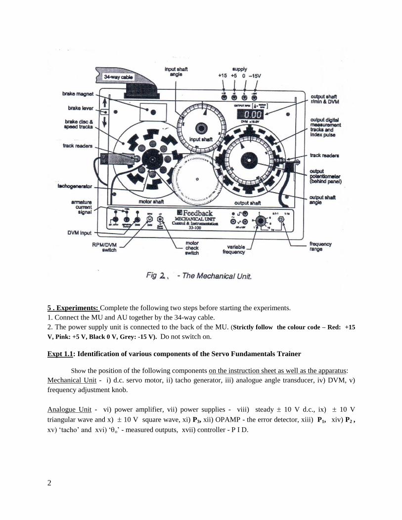
It consists of a Mechanical Unit (MU) and an Analogue Unit (AU).
Mechanical Unit (MU) houses a d.c. servo motor. Shaft of the motor carries a magnetic brake
disc, a tacho generator (speed transducer) and an output potentiometer (analogue angle transducer).
Motor drives shaft through a 32:1 belt reduction. On lower left corner of MU are meters for measuring
voltage, armature current and speed. A digital voltmeter (DVM) measures voltage/r.p.m. and displays it.
On MU are frequency adjustment knobs of the square and triangular waves in the Analogue Unit (AU).
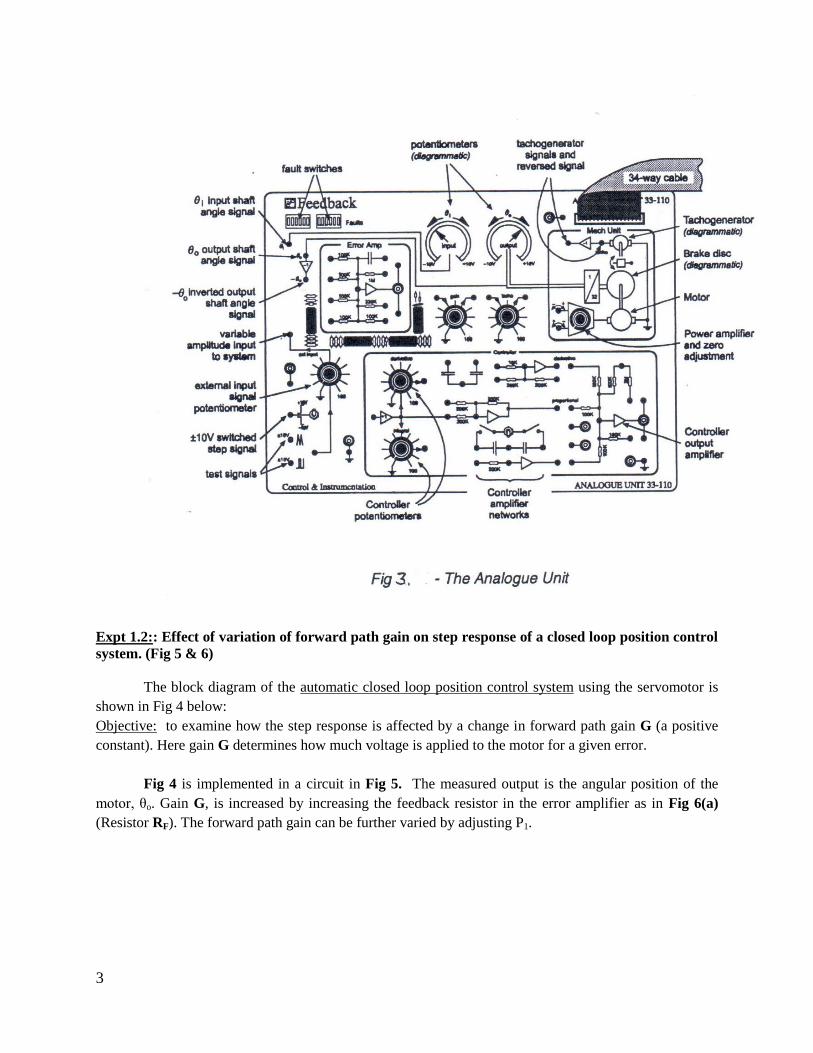
AU (Fig. 3) connects to the MU (Fig. 2) through a 32-way ribbon cable.
In AU the power supplies used as reference inputs – i) A steady 10 V d.c., ii) a 10 V
triangular wave and a 10 V square wave. SW is a three position switch (up, center and bottom) to
connect 10 V. The amplitude of these signals are varied through potentiometer P3.
On AU, OPAMP, A1, acts as an error detector. Potentiometers P1 and P2 control gains of the
system. Power amplifier, supplies the motor input voltage. Outputs of speed transducer (tacho
generator) and angle transducer (output potentiometer) are brought (from MU to AU at points „tacho‟
and „o‟ resp and are measured outputs (used for speed or position feedback ).
In lower part of AU lies controller, with proportional (P), Integral (I) and derivative (D) control -
implemented through OPAMPS, resistors and capacitors.
Fig 2 and 3 resp show schematic diagrams of the MU and AU. The Analogue Unit (AU) and the
Mechanical Unit (MU) can be combined to configure the basic system in Fig 1.
Error detector
+
_
Fig. 1 Analogue Control System
Input
Transducer
Amplifier Geared
Motor
Output
Transducer
2
5 . Experiments: Complete the following two steps before starting the experiments.
1. Connect the MU and AU together by the 34-way cable.
2. The power supply unit is connected to the back of the MU. (Strictly follow the colour code – Red: +15
V, Pink: +5 V, Black 0 V, Grey: -15 V). Do not switch on.
Expt 1.1: Identification of various components of the Servo Fundamentals Trainer
Show the position of the following components on the instruction sheet as well as the apparatus:
Mechanical Unit - i) d.c. servo motor, ii) tacho generator, iii) analogue angle transducer, iv) DVM, v)
frequency adjustment knob.
Analogue Unit - vi) power amplifier, vii) power supplies - viii) steady 10 V d.c., ix) 10 V
triangular wave and x) 10 V square wave, xi) P3, xii) OPAMP - the error detector, xiii) P1, xiv) P2 ,
xv) „tacho‟ and xvi) „o‟ - measured outputs, xvii) controller - P I D.
3
Expt 1.2:: Effect of variation of forward path gain on step response of a closed loop position control
system. (Fig 5 & 6)
The block diagram of the automatic closed loop position control system using the servomotor is
shown in Fig 4 below:
Objective: to examine how the step response is affected by a change in forward path gain G (a positive
constant). Here gain G determines how much voltage is applied to the motor for a given error.
Fig 4 is implemented in a circuit in Fig 5. The measured output is the angular position of the
motor, θo. Gain G, is increased by increasing the feedback resistor in the error amplifier as in Fig 6(a)
(Resistor RF). The forward path gain can be further varied by adjusting P1.
4
Fig 4 Block diagram of the closed loop system.
Procedure:
1. Connect the setup as in Fig. 5. Do not switch ON. It is a negative feedback arrangement using Error
Amplifier A1 (in differential mode) and potentiometer P1. The variable reference input comes from P3
and is connected to the input A of error amp A1. The measured output is the motor position and comes
from the θo output (after an inversion) to input B of A1. The output of A1, the error, (= reference-
measured value) is fed to P1 and finally to the power amplifier which supplies the motor. The circuitry
of the OPAMP A1 as an error detector is shown in Fig 6a. The gain of the OPAMP may be changed by
adjusting the feedback resistor RF.
2. Put P3 and P1 to zero position (rotate fully CCW).
3. Set the input square wave signal frequency to about 0.1 Hz.
4. Switch ON supply. Set P1 to zero. Adjust P3 = 3. Now turn P1 = 50 or until motor rotates freely.
5. Connect oscilloscope. Adjust its settings..Note value of RF , the rise time and overshoot in Table 1.
Roughly sketch the CRO response on paper.
6. Switch off supply.
7. Change RF to 330 kΏ. Switch ON. Repeat step 5. Switch off supply.
8. Change RF to 1 MΏ. Switch ON. Repeat step 5.
Expt 1.3 Automatic Position control of a d.c. servo motor by a P-D controller. (Fig 7a & 7b)
1. A control signal is obtained by combining the error, the derivative of the error and the integral of the
error – through a PID controller. The PID controller is implemented in the „Controller‟ section of the AU
through OPAMP with 1 F capacitor input, an OPAMP (acts as a „differentiator‟). With a 2 F capacitor
in the feedback path, an OPAMP acts as an integrator.
2. The error is produced by the OPAMP A1. The measured output is the motor position,0, coming from
an output potentiometer (after an inversion) to the input B of A1. The output of A1 is fed to the
Controller in AU. The forward path gain may be adjusted by changing P1 and the controller may be
configured for proportional (P), derivative (D) or/ and integral (I) action.
3. A circuit to realize P+D control is in Fig. 7(a) and the corresponding connections are given in Fig. 7(b).
G Geared Motor Power
Amplifier
Output
Transducer
5
Procedure:
1. Connect as in Fig. 7. Do not switch ON.
2. Connect the setup as in Fig. 7(b). Do not switch on.
3. Keep P1 = 0 and P4 = 0. Adjust the frequency of the square wave test signal to 0.2 Hz on the MU.
Switch on the power. Make P3 = 3.
4. Make P1 = 100 and P4 = 0 to get a forward path gain = 5 (check and explain). Adjust the CRO to
display the input and output waveforms. Take readings to fill up Table 2.
5. Roughly sketch the response.
6. Turn up P4 (derivative action increased) to 50 and note change in output response 0. Fill up Table 2.
7. Roughly sketch the response on the same axes as in step 5 (to note the change in response).
6
6. Report:
Expt no. 1.1:
1. Mark all the components on a (Xerox copy of) the schematic diagrams of the AU and MU.
Expt no. 1.2: i. State the effects of a change in the forward path gain G on the transient and steady state response.
iii. Comment on the stability of the open loop and closed loop systems.
iv. What device is used as the output transducer?
Expt. No. 1.3:
i. State the effect of the derivative action on transient response and tracking error in a single sentence.
7
Practice Questions (for labtest) i. In expt 1.2, for the diagram in Fig 4, find open loop and closed loop transfer functions (in terms of circuit
parameters) assuming suitable symbols for the motor parameters. (No need to search for numerical values.)
ii. Draw the block diagram of the circuit in Fig. 7(b).
iii. Calculate the gain of the OPAMPS in the P and the D sections of the Controller in Fig. 7.
References:
1. Automatic Control Systems – B. C. Kuo.
2. Control Systems Engineering, Norman S. Nise, John Wiley & Sons.
3. Manual of Servo Fundamentals Trainer, Feedback Ltd.
8
Table 1
Sl
No. RF Rise
time
Peak
overshoot
Gain of the Error
Amplifier
Nature of
damping
Rough Location
of CL poles
1. 100
K
2. 330
K
3. 1 M
Table 2
Sl
No.
P1 P4 Rise time Peak overshoot Change in response
1.
100 0
2.
100 50
Table 3
Sl. No. Item Make & model no.
1.
Analogue Unit
2.
Mechanical Unit
3.
Power Supply Unit
4.
Storage Oscilloscope
9
Control System Laboratory Experiment no.751/2
1. Title: STUDY OF A SYNCHRO BASED D.C. POSITION CONTROL SYSTEM
2. Object: To be familiar with a position control system comprising of error sensing synchro
devices, thyristorised amplifier, balanced bridge demodulator and DC separately excited
(actuator) motor.
Apparatus Used:
1. Synchro Generator:115/90 Volts, 60 Hz
2. Synchro Control Transformer:90/57.5 Volts, 60 Hz
3. Balanced Bridge Demodulator
4. DC Servo Motor and Reduction Gear Arrangement 110, 10A.
3. Theory: A d. c. motor is used to position any load mounted on its shaft. The reference
angular position of the load is given on the synchro generator (TX) rotor. The synchro control
transformer (CT) is mounted on the shaft of the motor and load. When the load is not
“positioned‟‟ (i.e there is a mismatch between the angular positions of the TX & CT), an error
voltage appears at the rotor terminals of the CT. This error voltage triggers the thyristors in a
way so that the d.c. motor is supplied with a voltage and the motor rotates in a direction to
nullify the error voltage. In this way the load is positioned according to the reference position.
Depending upon the reference position (angular) of synchro TX, the position control
system must be able to drive the controlled d. c. motor shaft to the required angle.
Hence the error in angular position is sensed by synchro TX-CT system comprising of
synchro generator and synchro transformer. Since the driving motor is a d.c. separately excited
motor, speed control in both directions is achieved by controlling armature voltage. A
thyristorised converter is used as the power amplifier capable of supplying armature current in
both directions (Dual converter). #
Note 1.
4. Procedure:
1. Note that an external armature resistance is connected to the d.c. motor.
Expt 4.1 Identify i) power amplifier block, ii)synchro error generator block, iii) demodulator
block and iv) path of flow of armature current and v)thyristor triggering current in the circuit
diagram.
3. Now make the error voltage zero by shorting the error voltage input terminal on the controller
board and make sure that the synchro control transformer output is not shorted.
11
5. Now the controller is ready for further experiments.
6. Connect the error voltage from synchro CT to the error voltage terminal on the controller
board. Observe (by changing the TX input in steps) that the output shaft (CT shaft) follows
the input shaft (TX shaft) rotation in both the direction.
7. Apply a step change in the reference position and observe the response in the system.
Expt 4.2 Determination of Synchro Characteristics:
The motor is not allowed to rotate by short circuiting the armature. By varying the Synchro TX
reference angular position, tabulate the synchro control transformer output voltage in Table 1.
The armature resistance is present in the circuit to avoid short circuiting of the power amplifier.
Expt 4.3 Determination of the Controller Characteristics:
This procedure is followed like the previous one. With the same set of reference angle position
tabulate the DC voltage across the series (armature) resistance in Table 1.
Expt 4.4 Observation of the different waveforms:
With the motor not allowed to rotate, observe and trace the waveforms across i) across the
capacitance and ii) error signal by varying Input reference position in synchro generator for +300,
-300
and 00 values of firing angle of the thyristor.
5. Report:
1) Plot the Input/Output Characteristics of the synchro error generator.
2) Plot the Input/Output characteristics of the controller on the same graph paper.
3) Paste the traced waveforms with proper labeling and respective values.
4) Draw the illustrative waveforms showing the working principle of the controller.
Appendix:
Note 1: Since error signal is an alternating signal, the sense of rotation is derived from the phase
angle of the error signal w.r.t the reference signal. Therefore a phase sensitive demodulator is
incorporated (balanced bridge demodulator) before the power amplifying stage.
Procedure to balance the Controller:
1. Observe that the controlled disc may be rotating.
2. Keeping P3, P2 at maximum, adjust P1 such that the disc stops rotating. This is the method of
balancing the demodulator i.e with error voltage zero the disc must not rotate.
3. Slightly vary P1 and observe the sensitivity of the controller by observing the immediate
direction of rotation of the controlled disc. The disc will rotate in either direction whenever
the P1 is increased or decreased from the balanced condition. The sensitivity may be
increased by adjusting gain potentiometer (P2) and dead zone potentiometer (P3).
12
Table 1 (Expts 4.2 and 4.3)
Sl No. Reference Angular
Position of TX
( )
Error Voltage across CT
( )
Voltage Across Series
Resistance
( )
13
Control System Laboratory
Experiment no. 751/3
1. Title: DESIGN OF A LEAD COMPENSATOR FOR A STANDARD SECOND ORDER
SYSTEM
2. Objective: To be familiar with lead compensator design
3. Theory:
Set Under Test:
A second order plant is simulated (in hardware) using passive R-L-C components and OPAMPS
as shown below in Fig. 1. Its control system equivalent is also shown in Fig. 2.
Lead compensator:
A schematic diagram of an electrical lead network is shown in Fig. 3. The name “lead
network” comes from the fact that for a sinusoidal input ei, the output eo, the network is also
sinusoidal with phase lead. The phase lead angle is a function of the frequency
Lead compensation essentially yields an appreciable improvement in transient response.
4. Experiments:
Expt 4.1 Design a lead compensator such that ωn is doubled but ξ remains unchanged. This
implies that rise time in the step response of compensated system will be halved while the peak
overshoot remains the same as that of the uncompensated one.
Procedure:
4.2.1. Insert values of ωn and ξ as given below:
ωn = 5230 rad/sec (4.1)
ξ = 0.24 (4.2)
in the open loop transfer function G(s) (in Fig. 2):
)2()(
2
n
n
sssG
(4.3)
and find the closed loop characteristic polynomial by applying unity feedback around (4.3)
(without the compensator). Hence first obtain the existing closed loop poles, se1 and se2 of the
uncompensated plant (using ωn and ξ found in eqns (4.1) and (4.2) resp).
4.2.2. Next find the desired closed loop poles, sd1 and sd2 after making ωn double and keeping ξ
unchanged in (4.3) (i.e., in se1 and se2). Fill in Table 1.
15
4.2.3. Compensator design using Root Locus:
The compensator T.F. is given by:
Ts
TsK
sG
C
C
1
1
)(
i) Find the angle contribution θ, of the poles of G(s) (in (4.3)) at the point sd1.Note that since θ
is not an odd multiple of 180 deg., sd1 does not lie on the root locus.
ii) Now determine the angle φ, to be contributed by the lead compensator, to fulfill the angle
criterion at sd1. Hence to make sd1 lie on the root locus, i.e., to make it a closed loop pole,
φ + θ = -1800 (4.4)
Find φ from the above. Fill Table 1.
iii) Now make the following construction (Fig. 4) on a graph paper to locate the pole and zero of
the lead compensator:
Locate sd1 (found in step 4.2.2) on the s-plane at point P on an ordinary graph paper (choosing
the same enlarged scale in x and y axes so that the entire graph paper covers the second
quadrant). Draw line AP parallel to the x-axis. Line PB bisects the angle OPA. Draw two lines
PC and PD making angle φ/2 with the bisector PB. C and D respectively give the locations of
the pole and zero of the lead compensator. Fill up Table 2.
Value of C = location of compensator zero
Value of D = location of compensator pole
iv) To find KC: the forward path transfer function of the compensated system is given by,
GOL(s) = KCGc(s) G(s)
KC is the gain of the amplifier (in the lead compensator) included to fulfill magnitude criterion at
sd1. To make sd1 a closed loop pole, KC is to found from: -
1)()( 11 ddCC sGsGK (4.5)
and fill in Table 2.
4.2.4 Fabrication of the Compensator: The compensator circuit given in Fig. 3 may now be
fabricated using the values obtained in steps (iii) and (iv). Choosing C = 1 μF and R3 = 1 KΩ,
choose R1, R2 and R4 from nearest available standard ones. Fill up Table 3. Now fabricate the
lead compensator along with the OPAMP on a bread-board. Required power supplies for the IC
are available on the experimental setup.
4.2.5 Validation of design: Attach the compensator to the experimental setup. Observe on a
CRO and roughly sketch the step responses of the system with and without compensation (on
same axes). Take readings to complete Table 4.
16
Table 1
Existing closed loop
poles
se1
Desired Closed Loop
Poles
sd1
Angle Contribution of
the Open Loop pole and
Zero at sd
Θ
Angle to be
Compensated
ø
Table 2
Compensator Zero
Compensator Pole
Compensator Gain
KC
Compensator Transfer
Function
Gc(s)
Table 3
Components Calculated Value Actual Value Used
R1
R2
R3
R4
C
Table 3
Peak Overshoot (%) Rise Time (secs)
Before compensation
After compensation
6.Report:
1. Produce the complete design steps showing all calculations made.
2. Attach rough sketches of the step responses of the compensated and uncompensated systems.
3. Comment on how far the design objectives could be fulfilled by you and the possible reasons
behind them. Could you use proportional gain only to fulfill the design objectives?
7. References:
1. Modern Control Engineering – K. Ogata (2nd
Edition)
2. Feedback Control System Analysis and Synthesis – J. J. D‟Azzo and C. H. Houpis.