– 1 –

DEPARTMENT OF HEALTH AND HUMAN SERVICES

Centers for Medicare & Medicaid Services

7500 Security Boulevard, Mail Stop N3-26-00

Baltimore, MD 21244

OFFICE OF THE ACTUARY

DATE: July 13, 2017

FROM: Stephen K. Heffler

Todd G. Caldis

Sheila D. Smith

Gigi A. Cuckler

SUBJECT: The Long-Term Projection Assumptions for Medicare and Aggregate National

Health Expenditures

The Office of the Actuary (OACT) annually produces 75-year Medicare expenditure projections

for the annual report of the Medicare Board of Trustees to Congress. The assumptions used in

the long-term projections have evolved over several decades through internal deliberations, four

independent technical advisory panel reports, ongoing discussions with the Medicare Trustees

and their staffs, and the input of various external researchers. This memorandum updates the

exposition of OACT’s long-range health spending projection methods used in the 2017 Medicare

Trustees Report.

Because of the significance of the long-range projections for public policy makers, it is important

for the projection assumptions to be as transparent and understandable as possible. The purpose

of this memorandum is to promote a more complete understanding of the long-range cost growth

assumptions by: (i) describing the projection challenge, (ii) providing a detailed description of

the current-law long-range assumptions, (iii) tracing the evolution of the long-range assumptions

used in the Trustees Report, and (iv) evaluating the strengths and limitations of the current cost

growth assumptions. Making such projections is not an exact science, and any long-term

projection model necessarily makes assumptions about the continuation of trends into an

uncertain future. The Office of the Actuary and the Board of Trustees continue to make every

effort to ensure that reasonable projections of Medicare’s future are included in the Trustees’

annual report.

The Long-Range Projection Challenge

Federal law requires the Medicare Trustees to report annually to Congress about the financial

and actuarial status of the Medicare program. OACT provides professional technical assistance

to the Trustees in their preparation of this report. Financial solvency determinations, defined

conceptually as measurement of the adequacy of projected program revenues to pay for projected

program obligations under current law, are reported for the Medicare trust funds.

In general, long-term projections, which span 75 years beginning with the current year, are made

under an assumption that existing institutional arrangements and program parameters embodied

in current law will prevail for the entire projection period. The 75-year “current-law” projections

– 2 –

are intended to reflect a policy-neutral baseline that is useful for policy makers, researchers,

health-care providers, beneficiaries, and others in considering the need for changes or

adjustments in national policy.

Both the time horizon and the institutional perspectives employed in long-term projections have

on occasion been criticized as unrealistic. Some observers have argued that projections

extending far into the future are so uncertain as to be of limited value and that a current-law

perspective assumes the perpetuation of existing policy arrangements beyond any reasonable

point. But such criticisms overlook a fundamental premise of long-term solvency reporting; that

is, projecting the long-term consequences of the institutional status quo affords decision makers a

reasonable opportunity to investigate trends, to consider alternatives, and to implement well-

conceived policy adjustments before financial or programmatic challenges reach crisis

proportions. Moreover, in view of the long-range financial commitments made by the Medicare

program,1 many would argue that it is critical to take every step to help ensure that these

commitments can be fulfilled, starting with a long-range evaluation of the financial status of

Medicare.

Long-range projections of Medicare revenues that appear in the Trustees Report are produced

using various long-range economic and demographic assumptions such as the size and age

distribution of the population, the size of the work force, average earnings levels, and the Gross

Domestic Product (GDP). These economic and demographic assumptions are determined

annually by the Social Security and Medicare Board of Trustees based on recommendations by

the Office of the Chief Actuary at the Social Security Administration. Projection of long-term

Medicare and aggregate national health expenditures by the Office of the Actuary at the Centers

for Medicare & Medicaid Services follows a similar process, but involves additional assumptions

that have been especially challenging to formulate and to validate.

The most difficult challenge in making long-range health expenditure projections is in

determining if and when a sector of the economy with a long history of rapid cost growth will

stabilize relative to the rest of the economy. Since the mid-20th century, the U.S. health sector

has grown substantially faster than the economy as a whole. As Chart 1 shows, since 1960 the

health sector's share of all of the nation's economic activity has increased by a factor of roughly

3.5 (from 5 percent in 1960 to nearly 18 percent in 2015). Given that the U.S. economy as a

whole has experienced more than fivefold real growth since 1960, the health sector has

experienced nearly a nineteen-fold increase (5 times 3.5) in real spending over the past 56 years.

The share of national output that the U.S. health sector absorbs has long, and by far, exceeded

1 As an example, consider new entrants to the workforce at age 20. If these individuals work and pay Hospital

Insurance payroll taxes on their earnings for a sufficient period, then they will qualify for HI benefits at age 65 (or

earlier, if they become disabled). Once enrolled at 65, these beneficiaries may live for another 30 years or more. In

this way, Medicare makes financial commitments that span at least the next 75 years.

– 3 –

the health sector share of any other developed nation, as shown in Chart 2, and there is no

evidence that the status of the U.S. relative to other developed nations will end.

Chart 1—National Health Expenditures (NHE)

as a Percentage of Gross Domestic Product (GDP)

1960-2015

Source: Centers for Medicare & Medicaid Services, Office of the Actuary.

0%

2%

4%

6%

8%

10%

12%

14%

16%

18%

20%

1960 1964 1968 1972 1976 1980 1984 1988 1992 1996 2000 2004 2008 2012

NHE

Share

of

GDP

(%)

Year

– 4 –

Chart 2—CY 2015 Health Expenditures as a Share of GDP

Selected OECD Countries

5.2

5.6

5.8

6.3

6.3

7.0

7.0

7.2

7.2

7.4

7.5

7.7

8.2

8.4

8.8

8.9

9.0

9.1

9.3

9.4

9.4

9.6

9.8

9.9

10.1

10.4

10.4

10.6

10.8

11.0

11.111.1

11.2

11.5

16.9

0 2 4 6 8 10 12 14 16 18 20

Turkey

Latvia

Mexico

Estonia

Poland

Slovak Republic

Hungary

Luxembourg

Korea

Israel

Czech Republic

Chile

Greece

Slovenia

Iceland

Portugal

Spain

Italy

Australia

Ireland

New Zealand

Finland

United Kingdom

Norway

Canada

Austria

Belgium

Denmark

Netherlands

France

Sweden

Germany

Japan

Switzerland

United States

Source: OECD Health Data 2017

Note: For the United States the 2015 data reported here do not match the 2015 data point for the United States in Chart

1 since the OECD uses a slightly different definition of “total expenditures on health” than that used in the United

States National Health Expenditure Accounts.

– 5 –

One way of analyzing health spending trends is to compare the growth rate of the U.S. health

sector with that of the overall economy. Using a definition of “excess cost growth” as the

difference between (i) the U.S. per capita growth rate in age-gender-adjusted health-care costs

and (ii) the per capita growth rate in GDP (both in constant dollars), Table 1 shows average

excess cost growth rates for selected time periods since 1975. Average excess cost growth rates

for national health expenditures (NHE) exhibit some volatility depending on which time periods

are used for defining averages, but over the long run this differential has generally been above 2

percent per year or just slightly below this level. There are only two periods in which rates of

excess cost growth have clearly deviated from a long-term rate of 2-percent. One of those

periods, 1995-2000, coincided with the widespread adoption of managed care approaches to

delivery of health care in the 1990s, but that slowdown proved temporary as strong excess cost

growth reemerged after the turn of the century. In the wake of the Great Recession the economy

experienced several years of low excess cost growth, on average -0.3 for the five year period

ending in 2015. Although negative excess cost growth rates were observed in the years 2011-

2013, the rate turned positive again in 2014, and in 2015 it was 1.5 percent, near the 30-year

average. Whether the rate will again recede or whether regression to longer-term means has

taken place is still uncertain, but the turnaround observed in the past two years does at least raise

the possibility that the rates experienced in 2011-2013 were just another temporary deviation

from a long-term trend. If the historic annual excess cost growth rate were to continue

unchecked, the health sector would encompass most, if not all, of the U.S. economy within the

75-year reporting horizon.

Since a nation that produces only health care is an impossibility, any method for projecting long-

range U.S. national health expenditures should consider and take into account any factors that

would contribute to an eventual slowdown in long-term growth rates for the health sector, to the

degree deemed likely to occur under existing law. But available research is inconclusive

concerning how much of a long-term slowdown in growth rates might take place, the probable

timing of a slowdown, the mechanisms that would cause a slowdown, and whether a slowdown

is likely to occur under current law. How these questions are addressed profoundly influences

the outcome of the expenditure projection process.

Despite the difficulty and uncertainty involved in projecting long-range NHE and Medicare

costs, projections are required for considering whether the promises made to the working

population today can reasonably be expected to be fulfilled many years in the future. The

balance of this memorandum describes the long-range health care cost growth assumptions,

explains the history behind the evolution of those assumptions, and finally considers the

reasonableness of the assumptions.

– 6 –

Table 1 - Compound Excess Cost Growth Rates, Selected Time Periods 1975-2015

Time period

Compound Constant-Dollar,

Per Capita Growth Excess Cost

(rounded) NHE (rounded) GDP (rounded)

Periods beginning with 1975:

through 1980 (5 years) 4.8% 2.7% 2.1%

through 1985 (10 years) 4.8% 2.5% 2.3%

through 1990 (15 years) 5.1% 2.5% 2.6%

through 1995 (20 years) 4.6% 2.2% 2.4%

through 2000 (25 years) 4.3% 2.4% 1.9%

through 2005 (30 years) 4.3% 2.3% 2.0%

through 2010 (35 years) 3.9% 1.9% 2.0%

through 2015 (40 years) 3.6% 1.9% 1.7%

Periods beginning with 1980:

through 1985 (5 years) 4.8% 2.4% 2.5%

through 1990 (10 years) 5.3% 2.4% 2.9%

through 1995 (15 years) 4.6% 2.1% 2.5%

through 2000 (20 years) 4.2% 2.4% 1.8%

through 2005 (25 years) 4.2% 2.2% 2.0%

through 2010 (30 years) 3.7% 1.8% 1.9%

through 2015 (35 years) 3.4% 1.7% 1.6%

Periods beginning with 1985:

through 1990 (5 years) 5.7% 2.4% 3.3%

through 1995 (10 years) 4.5% 1.9% 2.6%

through 2000 (15 years) 3.9% 2.4% 1.6%

through 2005 (20 years) 4.0% 2.2% 1.8%

through 2010 (25 years) 3.5% 1.7% 1.8%

through 2015 (30 years) 3.1% 1.6% 1.5%

Periods beginning with 1990:

through 1995 (5 years) 3.2% 1.4% 1.8%

through 2000 (10 years) 3.1% 2.4% 0.7%

through 2005 (15 years) 3.5% 2.1% 1.3%

through 2010 (20 years) 3.0% 1.5% 1.5%

through 2015 (25 years) 2.5% 1.6% 0.9%

Periods beginning with 1995:

through 2000 (5 years) 2.9% 3.3% -0.4%

through 2005 (10 years) 3.6% 2.4% 1.1%

through 2010 (15 years) 2.9% 1.6% 1.3%

through 2015 (20 years) 2.5% 1.5% 1.0%

Periods beginning with 2000:

through 2005 (5 years) 4.2% 1.6% 2.6%

through 2010 (10 years) 2.9% 0.7% 2.2%

through 2015 (15 years) 2.3% 0.9% 1.4%

Periods beginning with 2005

through 2010 (5 years) 1.6% -0.1% 1.8%

through 2015 (10 years) 1.4% 0.6% 0.8%

Periods beginning with 2010

through 2015 (5 years) 1.2% 1.3% -0.1%

Note: NHE rates were previously adjusted to remove age-gender effects on cost growth.

Source: Centers for Medicare and Medicaid Services, Office of the Actuary.

– 7 –

Long-Range Health Cost Growth Assumptions

This section summarizes the long-range excess cost growth assumptions used in the 2017

Trustees Report. Consideration of the history and reasonableness of the assumptions is deferred

until later sections.

The 75-year projections are constructed around the notion of excess cost growth, or the degree to

which growth in Medicare or health expenditures generally is expected to exceed the growth rate

of GDP. Excess cost growth is an intuitively understandable indicator of when a particular

sector is increasing in size relative to the rest of the economy. By definition, as long as a sector’s

rate of cost growth exceeds that of GDP, that particular sector (such as health care) will be

increasing as a share of the nation’s total economic output. As noted earlier in the discussion of

Table 1, one way of measuring excess health cost growth is as a difference of rates of growth:

the rate of age-gender-adjusted, per capita health care cost growth minus the rate of per capita

GDP growth.2

It is important to recognize that 75-year projections are only partially based upon long-run excess

cost growth assumptions. In the case of the first 10 years of the 75-year Medicare projections,

projections of costs are made separately for each category of health spending (for example,

inpatient hospital, physician, home health care, etc.) and are built up from assumptions about

general price inflation, excess medical inflation for each category of spending, changes in

utilization of services, and changes in the “intensity” or average complexity of services. (These

methods are described in detail in the Medicare Trustees Report.) An implicit year-10 excess

cost growth rate can then be computed from the results of the short-range projections. Years 11

through 24 of the 75-year projection are computed on an excess cost growth basis using rates that

blend the excess cost growth rate implicit in the year 10 short-range projection and the long-

range excess cost growth rate expected to prevail in year 25. For the last 51 years of the long-

range projection (years 25 to 75), excess cost growth assumptions are derived using the output

from the factors contributing to growth model described in more detail in the next section.3

Each Medicare subpart has a unique implicit excess cost growth rate as of year 10 of the

projection. Prior to the Affordable Care Act (ACA), the separate tenth-year growth rates were

transitioned to the same long-range excess cost growth rate assumption in year 25, so that the

program would then be projected as having a common set of excess cost growth rates for years

25 to 75. This long-range rate of excess cost growth for Medicare was assumed to be similar to

2 Excess cost growth calculations can be performed either on a nominal dollar or a real dollar basis as long as the

approach chosen is consistently applied. The long-range projections have always been computed on a nominal

dollar basis. In the actual development of the long-range projections, excess cost growth is computed on a

multiplicative basis fully consistent with the additive framework presented here. For a detailed explanation of the

implementation of excess cost growth computations see the Notational Appendix of the May 12, 2009 Projections

Methodology memorandum “The Long-Term Projection Assumptions and Aggregate National Health

Expenditures” at http://www.cms.gov/Research-Statistics-Data-and-Systems/Statistics-Trends-and-Reports/

ReportsTrustFunds/Downloads/ProjectionMethodology.pdf

3 As described subsequently in this memorandum, the growth assumptions can be derived either directly in the form

of excess growth rates (for example, using the traditional “GDP+X” framework) or by applying the statutory

provider payment rate updates to projected rates of growth for the utilization and intensity of medical services.

– 8 –

the excess cost growth rate prevailing for the rest of the U.S. health sector. Current-law price

provisions of the ACA, which require permanently slower annual payment updates relative to

prior law for many Medicare payment systems, mean that it is no longer feasible to transition to a

single excess cost growth rate for the entire Medicare program. Additionally, the enactment of

the Medicare Access and CHIP Reauthorization Act (MACRA) of 2015 specifies physician

payment updates with new incentives that replace payments previously determined by the

sustainable growth rate (SGR). As a result, long-range assumptions of underlying medical price

and quantity trajectories for each Medicare subpart are now developed from which excess cost

growth rates can be computed.

In particular, for the last 51 years of the 75-year period, growth assumptions are developed for

overall national health spending, and these assumptions are used in the development of separate

Medicare spending assumptions for Part A, certain subsets of Part B, and Part D. A description

of the overall national health spending assumption is discussed below, followed by a detailed

description of the methodology used for determining the long-range Medicare spending growth

assumptions for Medicare Part A, Part B, and Part D.

Overall National Health Expenditures (NHE)

The long-range projection starts with the assumption that overall per capita health spending will

increase on a year-by-year basis at rates determined using the Office of the Actuary’s “factors

contributing to growth” (FCG) model. The FCG model is an assumptions-based approach in

which the historical impact of key drivers of national health spending growth are used to inform

expectations about the long-run future, including the long-range implications of an increasing

share of our economic resources being devoted to health spending. The model is an extension of

the basic factors analysis used by the 2000 Medicare Technical Review Panel. It draws on the

additional data available since 2000 as well as refinements to the economic literature on the

factors underlying health care cost growth—specifically, changes in national income, relative

medical price inflation, health insurance coverage, and residual effects, which are primarily the

impact of innovations in medical technology.4 (Appendix A describes the FCG model in detail.)

Overall health spending is used as a starting point in developing the Medicare assumption since a

significant amount of research is available decomposing the drivers of overall health spending

trends (both for the U.S. and other countries), and it is assumed that over the long run that those

drivers would be generally similar across the health sector.

The per capita increase in health care costs reflects the combined effects of general inflation,

medical-specific “excess” price inflation (medical price inflation above general price inflation),

and changes in the utilization of services per person and the “intensity” or average complexity

per service. General inflation, as measured by the GDP deflator, is assumed to increase 2.2

percent per year over the long-range period. Relative medical price inflation for the overall

health sector is assumed to grow at 0.8 percent annually based on the difference between the

change in the personal health care deflator from 1990 to 2015 and the change in the GDP

4 Sheila Smith, Joseph Newhouse, and Mark Freeland, “Income, Insurance, and Technology: Why Does Health

Spending Outpace Economic Growth?” Health Affairs, September/October 2009 28:1276-1284.

– 9 –

deflator over the same period. Combining the projected 2.2 percent general inflation growth

with the assumed 0.8 percent relative medical price inflation results in medical sector output

price growth of 3.0 percent per year. The medical price change can be decomposed into its two

main factors5: (i) the prices paid for inputs to the production of medical care (e.g., employee

compensation, medical equipment, structures), or medical input price growth and (ii) the

efficiency with which those inputs are combined to produce medical care, or resource-based

health sector multifactor productivity growth.6 Resource-based health sector multifactor

productivity is assumed to grow at a pace consistent with published historical rates for hospitals

and physicians,7 and to average roughly zero for all other provider categories, such as skilled

nursing facilities, home health agencies, hospices, diagnostic laboratories, dialysis centers,

ambulance companies, etc. In aggregate for the overall health sector, resource-based health

sector multifactor productivity growth is estimated to be 0.4 percent per year. Thus, the medical

input price growth for the overall health sector, therefore, is assumed to be 3.4 percent per year.

Finally, the growth in the volume and intensity of services is determined as a function of three

key elasticity coefficients that influence the demand for health care:

1) Income-technology elasticity, which represents the marginal increase in demand for

health care and new medical technologies in response to growth in income. The income-

technology elasticity is estimated at 1.6 on average for the historical period from 1980

through 2002. It exhibits a declining trend over time, and is projected to reach 1.4 by

2015. This estimate is based on cross-country comparisons of the relationship of health

spending and GDP growth for member countries in the Organization for Economic Co-

operation and Development (OECD).8 A similar elasticity estimate was found using U.S.-

specific time-series data.

In the 2017 Trustees Report it is assumed that the elasticity for the 25th year of the

projection period (2041) is 1.26 and declines at a slowing pace to reach 1.09 by the end

of the 75-year projection period (2091). This assumption implies that, as health care

continues to consume a greater proportion of income, the marginal demand for additional

spending on health care and new medical technologies will lessen. Ultimately, health

5A third factor, the level of provider profit margins, is assumed to remain unchanged over the long run.

6Resource-based productivity is defined as the real value of provider goods and services divided by the real value of

the resources (inputs) used to produce the goods and services, where price changes are measured across constant

products—that is, defined health services with a constant mix of inputs. Resource-based productivity is used for this

decomposition, rather than outcomes-based productivity (which incorporates the estimated value of improvements in

health resulting from the services) because Medicare and most other payers reimburse providers based on their

resource use.

7Information on updated estimates of hospital productivity is available at https://www.cms.gov/Research-Statistics-

Data-and-Systems/Statistics-Trends-and-Reports/ReportsTrustFunds/Downloads/ProductivityMemo2016.pdf. Estimates of physician productivity are available here: Fisher, Charles: “Multifactor Productivity in Physicians’

Offices: An Exploratory Analysis.” Health Care Financing Review 29(2): 15-32, Winter 2007-2008.

8 The elasticity was estimated based on OECD data for 1970-2012 using rolling 21-year sample intervals to evaluate

the trend in the parameter over time. For additional detail, please see Appendix A.

– 10 –

care spending, including access to new technologies, is assumed to become a “normal

good,” rather than a “superior good.” As medical care consumption requires a steadily

increasing share of total income, demand for additional medical care at the margin is

likely to taper off.

2) Medical price elasticity, which reflects the sensitivity of patients and purchasers in

consuming health care to rising prices for medical care in relation to all other goods. The

assumption for this measure is premised on a decomposition of the price elasticity to

capture the increasing sensitivity of demand for health care to price in response to a rising

share of income accounted for by health care.9 Based on these considerations, the price

elasticity is estimated at −0.51 in the 25th year of the projection (2041) and follows a

non-linear path until it reaches −0.59 by the end of the 75-year projection period (2091).

3) Insurance elasticity, which reflects the change in demand for medical care as the level of

insurance coverage changes. Based on the RAND Health Insurance Experiment, this

elasticity is estimated at −0.2, reflecting the change in demand for health care as the

average coinsurance rate changes.10 For the 2017 Report of the Trustees, the insurance

elasticity is assumed to be unchanged over the long-range projection period at −0.2.

Additionally, the content of the insurance coverage is assumed to be unchanged over the long run

in order to maintain consistency with a Medicare benefit package that is unaltered.

Based on the year-by-year growth rates determined from the FCG model, age-gender adjusted

per capita national health spending is projected to grow at a rate of GDP plus 0.9 percent (or 4.8

percent) for 2041, gradually declining to GDP plus 0.5 percent by 2091 (or 4.3 percent).

Current Law Medicare Spending

The Trustees have assumed since 2001 that it is reasonable to expect over the long range that the

drivers of health spending will be similar for the overall health sector and for the Medicare

program. This view was affirmed by the 2010-2011 Medicare Technical Review Panel, which

recommended use of the same long-range assumptions for the increase in the volume and

intensity of health care services for the total health sector and for Medicare.11 Therefore, the

overall health sector long-range cost growth assumptions for volume and intensity are used as the

starting point for developing the Medicare-specific assumptions under current law.

Prior to the ACA, Medicare payment rates for most non-physician provider categories were

updated annually by the increase in providers’ input prices for the market basket of employee

9 This decomposition of the price elasticity is based on the Slutsky equation (see Silberberg, Eugene, The Structure of

Economics: A Mathematical Analysis, McGraw-Hill, 2000.) The relationship between the price elasticity and the

health share of GDP is estimated iteratively on a year-by-year basis to maintain internal consistency between the price

elasticity and the health share of GDP. 10Newhouse J, Health Insurance Experiment Group. Lessons from the RAND Health Insurance Experiment.

Cambridge (MA): Harvard University Press; 1993. 11 The Panel’s final report is available at https://aspe.hhs.gov/pdf-report/review-assumptions-and-methods-medicare-

trustees’-financial-projections.

– 11 –

wages and benefits, facility costs, medical supplies, energy and utility costs, professional liability

insurance, and other inputs needed to produce the health care goods and services. To the extent

that health care providers can improve their productivity each year, their net costs of production

(other things being equal) will increase more slowly than their input prices. Accordingly, since

most Medicare price updates prior to the ACA were equal to the increase in providers’ input

prices, Medicare costs per beneficiary would increase somewhat faster than for the health sector

overall. Because the market basket increase was assumed to be 3.4 percent annually, Medicare

payments grew about 0.4 percent greater than the net price increase of 3.0 percent per year

described above for the total health sector. The ACA requires that many of these Medicare

payment updates be reduced by the 10-year moving average increase in private, non-farm

business multifactor productivity, which the Trustees assume will be 1.1 percent per year over

the long range. The different statutory provisions for updating payment rates require the

development of separate long-range Medicare cost growth assumptions for four categories of

health care providers:

(i) All HI, and some SMI Part B, services that are updated annually by provider input price

increases less the increase in economy-wide productivity.

Combining the assumed market basket increase of 3.4 percent with the estimate of economy-

wide multifactor productivity, the statutory price update for these services is 2.3 percent per

year over the long-range projection period. The initial projected increase in the volume and

intensity of these Medicare services is assumed to be equivalent to the average projected

growth in the volume and intensity of services for the overall health sector. The Trustees

believe that the use of a common baseline rate of volume and intensity growth is reasonable,

as there would be only a small likelihood that one part of the health sector could continue to

grow indefinitely at significantly faster rates of growth than do other parts.

Additionally, the Trustees assume that the growth in Medicare payment rates under current

law will reduce the volume and intensity growth of these services by 0.1 percent per year

relative to the assumption from the factors model. The Trustees’ assumption is also based on

recommendations by the 2010-2011 Medicare Technical Review Panel, which concluded that

there would likely be a small net negative impact on volume and intensity growth due to

reduced incentives to develop new technologies, provider exits, and the impact of greater

bundling of services for payment purposes.12 For new technology that leads to new services,

the ACA will result in lower fees than would otherwise be the case, and providers will be less

likely to adopt new services and innovations, thereby lowering the demand for, and intensity

of, the medical care provided. Regarding provider exits, as fee-for-service fees decline relative

to the pre-ACA levels, facilities of marginal profitability are likely to exit the Medicare market,

reducing capacity and volume. This change could also cause a more bifurcated health system

to evolve in which only providers who can operate profitably under Medicare offer services to

Medicare beneficiaries, with a tendency to provide only the more basic services not associated

12 Other factors, such as reduced beneficiary cost-sharing requirements, would tend to increase the volume and

intensity of services. The assumption of −0.1 percent reflects the Technical Panel’s assessment that the overall impact

would be a small net decrease in volume and intensity growth.

– 12 –

with new medical technologies. Finally, the innovations being tested under the ACA, such as

bundled payments or accountable care organizations, could reduce incentives to adopt new

technologies for those participating in these programs and/or could contribute to greater efforts

to avoid services of limited or no value within the service bundle.

Reflecting all of these considerations, the year-by-year long-range cost growth assumption for

these HI and SMI Part B services starts at 3.9 percent in 2041, or GDP plus 0.0 percent, and

gradually declines to 3.5 percent by 2091, or GDP minus 0.3 percent.

(ii) Physician services

MACRA specifies physician payment updates with new incentives that replace payments

previously determined by the sustainable growth rate (SGR). Payments are assumed to increase

by 0.75 percent per year over the long run for those physicians participating in alternative

payment models (APMs) and 0.25 percent per year for those assumed to be participating in the

merit-based incentive payment systems (MIPS). The Trustees assume that the rate of per

beneficiary physician volume and intensity growth is based on the spending growth from the

FCG model and the price of physician services as measured by the Medicare Economic Index

(MEI). The year-by-year growth rates for physician payments are assumed to be 3.6 percent

in 2041, or GDP minus 0.3 percent, declining to 2.8 percent in 2091, or GDP minus 1.0 percent.

(iii) Certain SMI Part B services that are updated annually by the CPI increase less the increase

in productivity.

Such services include durable medical equipment, care at ambulatory surgical centers,

ambulance services, and medical supplies, which are updated by the CPI and affected by the

ACA productivity adjustment. For these services, the Trustees initially assume that the rate of

per beneficiary volume and intensity growth is equivalent to that derived for the overall health

sector using the factors model. This volume and intensity growth is assumed to be reduced by

0.1 percent per year to reflect the ACA impact, as described above. The post-ACA volume and

intensity assumption is combined with the long-range CPI assumption (2.6 percent) minus the

productivity factor (1.1 percent) to produce a long-range growth assumption for these SMI Part

B services. The corresponding year-by-year growth rates are 3.1 percent in 2041, or GDP

minus 0.8 percent, gradually declining to 2.7 percent in 2091, or GDP minus 1.1 percent.

(iv) All other Medicare services, for which payments are established based on market processes,

such as prescription drugs provided through Part D and the remaining Part B services.

The Trustees assume that per beneficiary outlays for these other Part B services, which

constitute about 15 percent of total Part B expenditures in 2025, and for all Part D services

grow at the same rate as the overall health sector as determined from the factors model.

These services are assumed to grow similarly because their payment updates are determined

by market forces. The year-by-year growth rates are 4.8 percent in 2041, or GDP plus 0.9

percent, gradually declining to 4.3 percent by 2091, or GDP plus 0.5 percent.

After combining the assumed rates of growth from the four categories of Medicare Part B

services described above, the weighted average growth rate for Part B is 3.7 percent per year for

the last 50 years of the projection period, or “GDP minus 0.2 percent,” on average. When Parts

– 13 –

A, B, and D are combined, the weighted average growth rate for Medicare is 3.7 percent over

this same period. For each of Parts A, B, and D, the assumed growth rates for years 11 through

25 of the projection period are set by interpolating between the rate at the end of the short-range

projection period (2026) and the rate at the start of the long-range period described above (2041).

Chart 3 provides a visual presentation of the year-by-year excess cost growth for Medicare Part

A, Part B, and Part D under current law over the last 65 years of the projection period (2027-

2091), including the 15-year transition of excess cost growth to their starting long-range values

in 2041 together with their gradually declining path thereafter. During the transition, Part A and

Part B growth is not perfectly linear because the projected values of economy-wide multifactor

productivity vary somewhat from year to year.

After 2041, the downward slopes of the Part A, Part B and Part D excess cost growth are similar,

reflecting the similar income-technology and price elasticities. Part D nevertheless continues at a

higher level because it is exempt from ACA-mandated annual payment reductions to which the

other subparts are subject.

Chart 3—Medicare Projected Excess Cost Growth

Current Law

2027-2091

Part B Excess Rate

Part D Excess Rate

-0.5%

0.0%

0.5%

1.0%

1.5%

2.0%

2027 2037 2047 2057 2067 2077 2087

Exce

ss C

ost

Gro

wth

Rat

es

Calendar Year

Part A Excess Rate

Source: Centers for Medicare and Medicaid Services, Office of the Actuary.

NOTE: An excess cost growth is the rate of change in per enrollee costs relative

to the growth in per capita GDP. The chart displays projected long-term excess

cost growth for Medicare Subparts A, B, and D under the current law. Under

this scenario each of the subparts has its own unique series of excess cost growth

through the end of the 75-year projection horizon due to the different applicable

current law payment provisions. Excess cost growth displayed here do not

include additional spending changes attributable to factors such as age and

gender composition of the Medicare population, IPAB impacts.

– 14 –

The Trustees Report cautions that “In view of these issues with provider payment rates, the

Trustees note that the actual future costs for Medicare could exceed those shown in this report.”

To help illustrate the level of Medicare costs that could result if these elements of current law are

overridden, the Trustees asked the Office of the Actuary to prepare projections based on a

hypothetical alternative.13 These projections are shown in the 2017 Trustees Report and in a

supplementary memorandum by the Office of the Actuary. The illustrative alternative projection

is based on the assumption that the economy-wide productivity adjustments to Medicare

payment rates would be gradually phased down during 2020 to 2034 and replaced with

adjustments based on estimated health-specific provider productivity gains of 0.4 percent

annually beginning in 2034. Additionally, the illustrative alternative assumes that, starting in

2026, physician payments transition from a payment update of 0.6 percent to an increase of 2.2

percent beginning in 2041 and that the 5-percent bonuses for physicians in alternative payment

models do not expire. Readers should not infer from this any endorsement of this theoretical

alternative to current law by the Trustees, CMS, or the Office of the Actuary, but concern about

the long-term feasibility of the adjustments makes it advisable to consider what the state of the

world might look like if they should prove infeasible.

Chart 4 shows the assumed year-by-year excess cost growth for Medicare Part A, Part B, and

Part D over the last 65 years of the long-range projection period for the illustrative alternative

Medicare projection. Under this illustration, per beneficiary cost growth for most of Medicare is

assumed to transition from their 2027 values to an approximately common set of growth rates

based on the FCG model for overall per capita national health expenditures (before demographic

adjustments).14

13 More information on these concerns is available in Appendix C of the 2017 Medicare Trustees Report and in a

memorandum by John Shatto and Kent Clemens of the Office of the Actuary, “Projected Medicare Expenditures

under Illustrative Scenarios with Alternative Payment Updates to Medicare Providers.” These documents can be

found at the following links: http://www.cms.gov/Research-Statistics-Data-and-Systems/Statistics-Trends-and-

Reports/ReportsTrustFunds/Downloads/TR2017.pdf and http://www.cms.gov/Research-Statistics-Data-and-

Systems/Statistics-Trends-and-Reports/ReportsTrustFunds/Downloads/2017TRAlternativeScenario.pdf.

14 The one exception is Part B services updated by the CPI, which are assumed to have the same volume and

intensity growth as NHE but a lower price update than assumed for NHE since those services are not updated based

on the market basket concept.

– 15 –

Chart 4—Medicare Projected Excess Cost Growth

Illustrative Alternative

2027-2091

Part D Excess Rate

Part A Excess Rate

-0.5%

0.0%

0.5%

1.0%

1.5%

2.0%

2027 2037 2047 2057 2067 2077 2087

Exce

ss C

ost

Rat

e R

ates

Calendar Year

Part B Excess Rate

Source: Centers for Medicare and Medicaid Services, Office of the Actuary.

NOTE: An excess cost growth is the rate of change in per enrollee costs relative

to the growth in per capita GDP. The chart displays projected long-term excess

cost growth for Medicare Subparts A, B, and D under the illustrative alternative.

Under this scenario each of the subparts converges to a similar rate of excess

cost growth through the end of the 75-year projection horizon. Excess cost

growth displayed here do not include additional spending changes attributable to

factors such as age and gender composition of the Medicare population, IPAB

impacts.

The excess cost growth assumptions are unchanged under the illustrative alternative for Part D.

For Parts A and B, however, the growth rates are higher than assumed under current law

throughout the final 65 years of the projection.

History of the Medicare Trustees Long-Range Health Cost Growth Assumptions

Officially convened Technical Panels of distinguished economists and actuaries have reviewed

the long-range Medicare projection and reporting methods on four different occasions—in 1991,

2000, 2004, and 2010-2011.15 Accordingly, the years 1991, 2000, 2004, and 2010-2011 serve as

milestone years in the evolution of methods that are employed to project Medicare over a 75-

year reporting period. In addition, the projection assumptions and methods have reflected annual

reviews and reassessments by the Office of the Actuary and the staffs of the Board of Trustees.

From time to time, other events have affected the projections, such as the development of

15 The Secretary of Health and Human Services announced the reestablishment of the Technical Review Panel on

the Medicare Trustees Report in the February 19, 2016 Federal Register.

– 16 –

Actuarial Standard of Practice No. 32, Social Insurance16 and the requirements of the Medicare

Prescription Drug, Improvement, and Modernization Act of 2003 (MMA) for the Medicare

Trustees Report to compare projected growth rates for Medicare to those for aggregate national

health expenditures, private health insurance expenditures, and GDP.17 This section traces the

evolution of projection methods through regular and responsible consultation with recognized

subject matter experts and through thoughtful implementation of advice received in light of the

reporting responsibilities that exist.

A. Stage I: Basic Structure of Long-Term Projections

The first Trustees Reports for Medicare, issued in 1966, provided 25-year projections for the

Hospital Insurance (HI) trust fund and only 3-year projections for the Supplementary Medical

Insurance (SMI) trust fund. No longer-range projections of any kind were made by the Medicare

Trustees before 1983, although the Office of the Actuary prepared 75-year projections from time

to time for special analyses. In 1983, the Board of Trustees decided to report the substantial

increase in HI costs that could reasonably be expected for Medicare as a result of demographic

changes alone—in particular, the retirement and subsequent aging of the post-World War II

“baby boom” generation. Since existing research still had little to say concerning the likely long-

term path of health care spending as it might be affected by non-demographic factors, it was

determined that initial long-term projections would not explicitly take such factors into account.

Accordingly, starting in 1983 long-range HI projections were made under the assumption that

long-range costs per unit of service would increase at the rate of average hourly earnings. No

long-range projections for SMI were reported by the Medicare Trustees until after the

recommendations of the 1991 Medicare Technical Review Panel.

The 1991 Medicare Technical Review Panel was the first formally convened body to consider

long-range projection methods to be used in the Medicare Trustees Reports.18, 19 A fundamental

theme of the panel’s report is coordination of projection methods for HI and SMI in order to

facilitate a combination of the results into a comprehensive understanding of the status of the

entire Medicare program. The use of a 75-year projection period was affirmed because, for the

average person entering the workforce in any reporting year, this period of time will encompass

his/her years as a contributor to the HI fund and as a Medicare beneficiary. The panel thus saw a

75-year reporting horizon as a reasonable period of analysis for evaluating the financial ability of

the program to deliver benefits promised to beneficiaries from the inception of their working

lives. The panel found the use of short-term projections based on trends that are gradually

tapered to meet long-run growth assumptions to be reasonable. The panel cautiously endorsed

16 Available at http://www.actuarialstandardsboard.org/pdf/asops/asop032_149.pdf .

17 Section 801 of the Medicare Prescription Drug, Improvement, and Modernization Act of 2003 (Pub.L. 108-173,

117 Stat. 2066), 42 U.S.C. 1395i.

18 Before 2002 there was an annual Trustees Report for HI and another for SMI; since 2002 there has been a single

annual Trustees Report that includes all parts of the Medicare program.

19 Report on Medicare Projections by the Health Technical Panel to the 1991 Advisory Council on Social Security

(March, 1991: Washington, D.C.).

– 17 –

the long-range assumption that average HI payments per unit of service would grow at the same

rate as average hourly earnings and expressed similar approval for a long-range assumption that

per enrollee SMI costs would grow at the same rate as per capita GDP. With regard to each

long-run assumption, the panel recommended that regular monitoring for continuing plausibility

should occur.

The approach to long-range projections described in the report of the 1991 Technical Panel was

reflected in succeeding Medicare Trustees Reports up to and including the HI and SMI reports

for 2000. Consistent with the recommendation to coordinate the HI and SMI projections, the

annual reports starting in 1994 show 75-year projections of HI and SMI as percentages of GDP.

The nature of the long-range assumptions meant that HI and SMI would grow more rapidly as a

percentage of GDP in the first 25 years of the projection period than in the last 50 years. In the

case of HI, the assumption that increases in per unit of service costs would equal the rate of

increase of average hourly earnings in the last 50 years of the projection period meant that costs

would be relatively stable in the long run. Other long-range assumptions related to

demographics still allowed for substantial growth in HI’s share of GDP. In the case of SMI, the

long-range assumption meant that growth as a share of GDP would largely halt after the first 25

years, except to the degree that changing demographics would continue to boost SMI’s share of

GDP.20

Although the 1991 Technical Panel had not explicitly discussed implementation of an excess

cost growth method to model long-range Medicare costs, the elements of the method are

discernable in the panel report and in the subsequent reports of the Medicare Trustees. The long-

range assumption for SMI was effectually a “GDP+0” assumption that was substantially below

historic rates of SMI growth, a fact that had prompted the Technical Panel to recommend regular

review of the assumption and that evoked regular cautionary commentary in Trustees Reports

during the 1992-2000 period. And even though the long-range assumption for the HI growth rate

was not directly related to GDP, the idea of connecting HI’s growth to that of a macro-

economically important aggregate was present. On these foundations, moving to an explicit

excess growth method for long-range projections for all parts of the Medicare program would

prove to be a natural next step.

B. Stage II: Addition of the GDP+1 Projection Method

The 2000 Medicare Technical Review Panel deliberated extensively about the long-term rate of

health care cost growth and ultimately recommended an assumption of tying Medicare’s long-

range cost growth to the increase in per capita GDP plus 1 percentage point (GDP+1), exclusive

of age-gender effects, for both HI and SMI. The panel viewed its mission as one of delivering

credible and usable assumptions concerning an inherently uncertain issue. The conceptual

innovation was in seeing the long-range assumption for both HI and SMI as explicitly a question

of the rate of excess cost growth relative to GDP under current law. Within the conceptual

20 The resulting projection pattern of HI growth versus SMI growth as a share of GDP is illustrated in Table III.B.1

of the 2000 HI Trustees Report.

– 18 –

framework, the practical task for the panel became a matter of arriving at a consensus for the

value to assign to the key projection variable that had been defined.

To achieve a consensus, the experts considered many factors that are thoroughly documented in

their written report.21 Most telling for the panel were long-term time-series expenditure trends

when considered in light of causal evidence. Long-term time-series evidence showed that in any

multi-year time period examined by the Technical Panel, real per capita health expenditures had

never grown at a rate less than 1 percent in excess of real per capita GDP growth. As for

determinants of expenditure growth, the panel looked to aggregate and micro-level health

economics studies, which pointed to technological change as the primary driver of real growth in

health expenditures. The panel report concluded that technological change alone would account

for a percentage point of real growth in excess of the rate of real GDP growth.

Also considered by the panel were factors that might in the future slow or accelerate the rate of

excess medical expenditure growth through the diffusion of technological change. For example,

the spread of managed care in the 1990s was seen as a short-term aberration in a long period of

excess cost growth relative to GDP growth rates and, thus, as unlikely to have an enduring effect.

The experts did not find evidence for a long-term differential among types of payers that would

affect their conclusion about the long-term excess growth rate. The panel also noted that other

forecasters showed a range of excess growth in health expenditures of between 0.8 to

1.5 percentage points, with most of the studies congregating around a value of 1 percentage

point.

Finally, the panel’s report discussed the sustainability of excess cost growth of 1 percent for the

duration of a 75-year projection period. Concerning this issue, the report noted that excess

growth of 1 percent per year over 75 years would lead to a health sector of unprecedented size as

a share of the economy, but since such a growth pattern would still be consistent with increases

in the absolute level of real consumption for non-health expenditure, the panel saw little grounds

for expecting consumers as a group to reach some point of satiety concerning health

expenditures.

Based upon their thorough review of relevant factors, the 2000 Technical Panel unanimously

recommended adoption of a long-term excess cost assumption of a full percentage point of

excess growth in per enrollee HI and SMI costs above the rate of growth of per capita GDP,

exclusive of age-gender effects. Their recommendation was supported by the Office of the

Actuary in its assumption recommendations in the Fall of 2000 to the last Medicare Board of

Trustees under the Clinton Administration and was adopted formally by that Board. With the

changes in Board membership under the incoming Bush Administration, the Office of the

Actuary again recommended the GDP + 1 long-range growth assumption, and it was again

adopted by the new Board and implemented in the 2001 Medicare Trustees Reports.22 As was to

21 Review of Assumptions and Methods of the Medicare Trustees’ Financial Projections by Technical Review Panel

on the Medicare Trustees Reports (Baltimore: 2000) available at: http://www.cms.gov/ReportsTrustFunds/

downloads/TechnicalPanelReport2000.pdf

22 By law, the members of the Medicare (and Social Security) Board of Trustees are the Secretary of the Treasury,

Secretary of Labor, Secretary of Health and Human Services, Commissioner of Social Security, and two members

– 19 –

be expected, the change to a more costly long-term assumption had a substantial effect on the

reported financial status of the Medicare program. In 2001, the Medicare share of GDP at the

end of 75 years was projected at 8.49 percent, as compared with 5.28 percent projected in the

2000 Report. The GDP+1 assumption as applied in the 2001 HI and SMI Trustees Reports was

also used in the annual reports issued from 2002 through 2005.

C. Phase III: Refinement of the GDP+1 Projection Method

A new Medicare Technical Panel was convened in 2004; it reviewed and reaffirmed the long-

term GDP+1 assumption as implemented by the Office of the Actuary, but also made

suggestions for research into long-term projection methods.23 In addition, the MMA required

that the Medicare Trustees compare past and projected Medicare cost growth rates with annual

rates of growth in GDP, private health insurance costs, national health expenditures, and other

appropriate measures. Together, the changes in statutory reporting requirements and the

suggestions of the 2004 Technical Panel provided impetus for refinement of how the GDP+1

assumption was implemented.

The 2004 Technical Panel considered the analysis of excess cost trends that had appeared in the

report of the 2000 Technical Panel and found that analysis to be persuasive. The 2004 panel was

comfortable with the existing framework and concluded that the existing GDP+1 long-range

assumption was “within the range of the reasonable assumptions, given the limits of current

knowledge.” However, the panel also found future promise in extramural general equilibrium

modeling projects already in progress under the supervision and sponsorship of the Office of the

Actuary, and accordingly the experts encouraged the pursuit of additional research to build

insight into the behavioral dynamics underlying health expenditure growth.24

The Office of the Actuary eventually determined that yearly expected excess cost rates for the

overall health sector, exclusive of age-gender effects, as derived from the constrained solution of

a stylized macroeconomic model—the OACT computable general equilibrium (CGE) model25—

could be used as a tool for improving the long-range Medicare cost growth assumptions and for

complying with new reporting responsibilities. A review of this approach by independent health

economists convened for this purpose confirmed this finding, and the OACT CGE model was

representing the public. Dr. John L. Palmer and Dr. Thomas R. Saving served as Public Trustees on both the 2000

and 2001 Boards of Trustees (as well as subsequent Boards through 2007).

23 Review of Assumptions and Methods of the Medicare Trustees’ Financial Projections by 2004 Technical Review

Panel on the Medicare Trustees Reports (Baltimore: December, 2004) available at: https://aspe.hhs.gov/pdf-report/

review-assumptions-and-methods-medicare-trustees’-financial-projections-0

24 The recommendation to explore many possible lines of insight with simple models was reiterated several years

later by members of an informal advisory group of distinguished economists and actuaries convened by the Office of

the Actuary in 2007.

25 The detailed structure of the model, but not how it was used in the Trustees Reports, is described in “Projecting long-term

medical spending growth,” by Christine Borger, Thomas F. Rutherford, and Gregory Y. Won, Journal of Health

Economics, Volume 27, Issue 1, pages 69-88 (2008).

– 20 –

adopted as a tool in the production of long-range estimates starting with the 2006 Medicare

Trustees Report.

The CGE model was used solely as a tool for developing a reasonable series of downward-

trending, year-by-year health care cost growth rates that were consistent with the constant

GDP+1 assumption used previously. A thorough review of the CGE model determined that

without exogenous identifying assumptions about the average rate of cost growth the model

could not be used as an independent forecasting tool. However, it made sense to use it as a tool

to translate the basic GDP+1 cost growth assumption into a financially equivalent series of

smoothly decelerating cost growth rates more consistent with a notion of diminishing marginal

utility of health care for a representative consumer as the budget share for health care increased.

D. Phase IV: Affordable Care Act

The enactment of the ACA in March 2010 required that several new provisions of the law be

taken into account when developing long-range Medicare projections. Most notably, the ACA

modifies the annual increases in Medicare payment rates for most categories of health service

providers by reducing them for 2011 and later by the 10-year moving average increase in private,

non-farm business multifactor productivity.26

For the 2010 and 2011 Medicare Trustees Reports, the Trustees first assumed a “baseline” set of

pre-ACA, long-range Medicare cost growth rates, using the methods described above regarding

the refinement of the GDP+1 method. This approach included continued use of the OACT CGE

model to determine the year-by-year growth rates consistent with an underlying average rate of

GDP plus 1 percent. These baseline long-range Medicare cost growth assumptions were then

altered to incorporate the payment adjustments associated with the ACA. This adjustment

affects all HI (Part A) providers; as a result, on average, the resulting long-range growth

assumption for HI was the increase in per capita GDP plus 1 percent, minus the productivity

factor (estimated at 1.1 percent per year). For SMI Part B, the productivity adjustment affects

certain provider categories—for example, outpatient hospitals, ambulatory surgical centers,

diagnostic laboratories, and most other non-physician services. These services had the same

assumed long-range growth rate as did HI services. The sustainable growth rate formula in

current law governed increases in average physician expenditures per beneficiary, so that they

would increase at approximately the rate of per capita GDP growth. The remaining Part B

services, and all Part D outlays, were not affected by the SGR or the ACA productivity

adjustments and had an assumed average growth rate of per capita GDP plus 1 percent

In its interim report, the 2010-2011 Medicare Technical Review Panel concluded that the

resulting long-range growth assumptions used in the 2010 and 2011 reports were not

unreasonable in light of the provisions of the Affordable Care Act.27

26 “Multifactor productivity” is a measure of real output per combined unit of labor and capital, reflecting the

contributions of all factors of production.

27 The Panel’s interim report is available at https://aspe.hhs.gov/review-long-range-assumptions-medicare-trustees-

projections-interim-report.

– 21 –

In December 2011, the panel members unanimously recommended a new approach that built off

of the longstanding “GDP plus 1 percent” assumption while incorporating several key

refinements. Specifically, the panel recommended use of two separate means of establishing

long-range growth rates:

The first approach is a refinement to the traditional “GDP plus 1 percent” growth assumption

that better accounts for the level of payment rate updates for Medicare (prior to the ACA)

compared to private health insurance and other payers of health care in the U.S. For

applicable provider categoriesthose with provider payment updates based on input price

increases, prior to the ACAthe refinement results in an increase in the long-range pre-ACA

“baseline” cost growth assumption for Medicare to “GDP plus 1.4 percentage points.” The

corresponding assumed average growth rate for aggregate national health expenditures

continues to be “GDP plus 1 percentage point.”28

The second approach recommended by the Technical Panel is the “factors contributing to

growth” (FCG) model developed by the Office of the Actuary at CMS as a possible

replacement for the existing process. This model also builds upon the key considerations

used in establishing the earlier “GDP plus 1 percent” assumption, together with subsequent

refinements in the analysis of growth factors, additional years of data on national health

expenditures available since the 2000 Technical Panel’s deliberations, and use of projected

trends in the model’s key factors. The model is based on economic research that decomposes

health spending growth into its major drivers—income growth, relative medical price

inflation, insurance coverage, and a residual factor that primarily reflects the impact of

technological development.29

For the 2012 Trustees Report, the long-range Medicare spending assumption was determined as

(i) a pre-ACA baseline assumption for the average ultimate Medicare growth rate using the

updated “GDP plus 1.4 percent” and (ii) the FCG model to create the specific year-by-year

declining growth rates during the last 50 years of the projection. These baseline assumptions

were then altered by the payment adjustments in the ACA.

For the 2013 and 2014 Trustees Reports, the long-range Medicare spending assumption was

determined based on (i) the volume and intensity assumptions derived from the FCG model,

(ii) the impacts on Medicare volume and intensity from the ACA, as recommended by the

Technical Panel, and (iii) the Medicare payment updates specified in current law. For the 2014

Report, an SGR override was assumed under the projected baseline scenario. For the 2015 and

2016 Reports, the passage of MACRA with a new payment system for Medicare physician

28 It is important to recognize that GDP+1.4 is prior to any multifactor productivity adjustment to Medicare

administrative payment systems as required by update provisions of ACA; the GDP+1 assumption for NHE is

consistent with negotiated provider payment rate updates that are net of provider productivity gains deemed to be

attainable across the health sector.

29 Smith, S., Newhouse, J., and Freeland, M., “Income, Insurance, and Technology: Why Does Health Spending

Outpace Economic Growth?” Health Affairs, September/October 2009.

– 22 –

services prompted a return to a current law perspective and a recalibration of certain FCG

parameters was implemented.

Evaluation of the Long-Range Cost Growth Assumptions

In this section the reasonableness of the key long-range assumptions and the projections that

result are discussed.

A. The NHE Projection Baseline

A core assumption underlying the OACT long-range health expenditure projections continues to

be that net per capita health expenditure growth for the U.S. health sector as a whole, exclusive

of age-gender effects, would experience a substantial slowdown from historic rates of excess cost

growth. Using the FCG model, the current assumption is that excess cost growth would be GDP

plus 0.9 percent for 2041, gradually declining to GDP plus 0.5 percent by 2091. The questions

to be considered here are whether the assumed cost slowdown inherent in the NHE assumption is

well-founded and whether it leads to a reasonable projection.

In approaching these questions, it is worth remembering that the term “excess cost growth” as

used by the Office of the Actuary is meant to be a descriptive rather than a normative term. In

other words, the term does not mean that there is anything intrinsically bad or inherently

unreasonable with faster growth for the health sector than for the rest of the U.S. economy. But,

as explained earlier in this memorandum, long-run historic trends in excess cost growth rates for

the health sector are ultimately unsustainable. The appropriate question regarding a long-range

projection is therefore what state of the world would be expected to prevail under a reasonable

set of assumptions about the evolution of the health sector.

The long-range assumptions about excess cost growth, together with demographic projections of

population size and age distribution, determine the magnitudes of the long-range projections.

Even if the long-range baseline assumptions are believed to be within the range of the

reasonable, it is fair to consider the degree to which the outputs are reasonable and credible.

Under the full illustrative alternative scenario, the health sector share of GDP is expected to

increase from 17.8 percent in 2015 to as much as 35.4 percent of GDP in 2091 (Chart 5). Such

magnitudes have no historical precedent and are even more extraordinary when it is considered

that these increased economic shares would be from an economy that, in real per capita terms, is

projected to be roughly three times the size that it is today.

– 23 –

Chart 5—National Health Expenditures as a Percent of GDP

1970-2091

0%

5%

10%

15%

20%

25%

30%

35%

40%

45%

1970 1980 1990 2000 2010 2020 2030 2040 2050 2060 2070 2080 2090

Shar

e o

f G

DP

(%

)

Calendar Year

NHE - Historic

NHE (Medicare CL)

NHE (Medicare Alt)

Source: Centers for Medicare and Medicaid Services, Office of the Actuary.

NOTE: Historical data is used before 2016 and projections from 2016 forward.

It is fair to question, as some researchers have, whether a future health sector of this size would

be macro-economically sustainable to the end of the 75-year projection horizon.30 When long-

range scenarios have been run by the INFORUM group at the University of Maryland, with their

detailed, bottom-up macroeconomic model (Long-Run Interindustry Forecasting Tool, or LIFT),

maintenance of current-law benefit levels has been found sustainable in the sense that some real

growth in the non-health sectors of the economy would still be feasible.31 But that analysis

purposely ignored macroeconomic “feedback effects” on investment, interest rates, and labor

supply from the increases in tax rates and/or government debt levels that would be needed to

finance Medicare and Medicaid.32 The more significant that those macroeconomic effects are,

the more likely a slowdown in Medicare excess cost growth even below the long-range

assumption. Distributional issues are also likely to emerge as Medicare Part B premiums and

30 Glenn Follette and Louise Sheiner, “The Sustainability of Health Spending Growth,” National Tax Journal,

Volume 58, pages 391-408 (2005).

31 Mark Freeland, Greg Won, Stephen Heffler, and Margaret McCarthy, “Issues on the Sustainability of Long-Term

Health Spending Projections,” Paper delivered at 2002 SGE/ASSA/AEA Conference session on “Long-Term

Projections of Health Care and Medicare Costs.”

32 When such factors were reflected in LIFT model runs, the macroeconomic impacts of tax increases and increased

federal borrowing resulted in long-range economic growth that was substantially slower than assumed in the

Trustees Reports.

– 24 –

cost sharing start to consume 50 percent or more of monthly Social Security benefits for some

beneficiaries.33

A National Academy of Sciences committee has also issued an important report about alternative

choices that the nation faces in order to make its system of entitlement programs, including

Medicare, fiscally sustainable.34 Various alternative scenarios, including scenarios involving

rates of growth less than GDP+1, are considered to underscore that there are choices to be made

to decide the nation's future, but no position is taken concerning which scenario would be

optimal.

Abundant reasons thus exist to question whether the long-range NHE projection baseline would

itself in fact be sustainable. Yet even though the sources cited here raise pertinent practical

questions about the ultimate sustainability of this current law scenario, none of them provides a

reliable basis for adopting a lower baseline. What is more, the persistence of high rates of excess

cost growth over history, despite previous legislative initiatives aimed at reducing it, is another

important inducement to caution in the adoption of a projection baseline.35 The NHE projections

are undoubtedly more realistic than assuming excess cost growth continues unabated at historic

trend rates, but the results are still large enough to underscore the need for effective policy

intervention if the growth of the U.S. health sector relative to the rest of the U.S. economy is ever

to be stabilized.36

B. The Relationship between NHE and Medicare Projections under Current Law

Recent Medicare Technical Review Panels have in one way or another been comfortable

assuming that average growth over the long-range projection period would be consistent with

slowing excess cost growth given that historic rates are simply unsustainable. However, the

panels have provided little analysis of specific mechanisms that might cause a slowdown of

excess cost growth. For example, the 2000 Technical Panel was impressed by evidence that an

excess cost growth rate of 1 percent (GDP+1) would still be consistent with maintaining some

positive real growth in an absolute sense in other sectors of the economy. Maintenance of

positive real growth in per capita non-health expenditures might therefore be interpreted as

defining an outer limit on social willingness to pay for additional health care.

How the U.S. economy in the absence of major policy interventions would in fact move from a

historic excess cost growth rate of GDP+2 remains a largely unsettled question. The existing

33 See Figure II.F2, 2017 Trustees Report, at page 37 available at: http://www.cms.gov/Research-Statistics-Data-

and-Systems/Statistics-Trends-and-Reports/ReportsTrustFunds/Downloads/TR2017.pdf.

34 Committee on the Fiscal Future of the United States, Choosing the Nation's Fiscal Future, The National

Academies Press, Washington, D.C., (2010), www.nap.edu

35 For instance, the Sustainable Growth Rate system that was supposed to control the growth of Medicare physician

fees was overridden by Congress nearly every year.

36 Even with zero or slightly negative excess cost growth, as in the current law Medicare projections, the Medicare

program will continue to grow as a share of the U.S. economy as long as the share of the population eligible for

Medicare benefits is increasing relative to the overall population.

– 25 –

Medicare program and private health insurance plans more generally contain numerous features

by which consumer preferences for slower expansion in health care could eventually reduce the

rate of excess cost growth in line with the expectations of the Technical Review Panels,

including the most recent panel.

By way of illustration, consider the potential effects of cost-sharing provisions of current-law

Medicare, which are more substantial and more extensive than is often recognized. 37 At present,

the great majority of Medicare beneficiaries (roughly 90 percent) have supplemental health

insurance coverage that helps insure against Medicare’s point-of-service cost-sharing

obligations. Such coverage is provided through supplemental private “Medigap” insurance

programs paid for by the beneficiaries themselves, participation in private Medicare Advantage

coordinated care plans, retiree health plans provided by their former employers, or the Medicaid

program. As the costs of comprehensive supplemental coverage rise relative to the growth of

personal income and business income, the comprehensiveness and the prevalence of such

coverage are likely to diminish, and point-of-service cost sharing faced by Medicare

beneficiaries is likely to become more frequent and more burdensome. Accordingly, as time

passes, beneficiaries may choose more frequently not to seek health care perceived by them to be

of limited marginal value or to decline health care offered by providers.

That cost sharing can have substantial effects on demand for health care is an established

proposition. The results of the well-known RAND Health Insurance Experiment persuasively

confirm that substantial effects on demand for health care arise from point-of-service cost

obligations borne by patients.38 Moreover, an important recent study indicates that the scope of

insurance coverage is likely to have had an even greater effect on health sector size than could be

identified by the study design used in the original RAND Health Insurance Experiment.39

Further consumption-side brakes on Medicare as excess costs accumulate might include

decisions not to enroll in Medicare Part B or Part D. Such individuals would face even more

substantial point-of-service obligations that would have significant effects on their access to

health care.

Over the past few decades the apparent role of cost sharing in the finance of health care has

diminished, mostly through the spread of public health insurance coverage and private

37 There is no provision in current law that would permit payment of full HI benefits after trust fund exhaustion.

Since the purpose of the Medicare and Social Security Trustees Reports is to evaluate the adequacy of program

financing, however, the Trustees have always made projections of (i) the benefits specified under current law (and

the associated costs of administering the program) and (ii) the revenues specified under current law. The annual

report then compares these two projections to evaluate whether financing is sufficient. Thus, the Trustees’

application of current law does not follow a strict interpretation of what would actually happen in the event of trust

fund depletion; rather, it compares expenditure and income levels under the implicit assumption that full benefits

would be paid. In practice, Congress has never allowed the HI trust fund to be exhausted, and it is highly likely that

action would be forthcoming to prevent exhaustion at a future date.

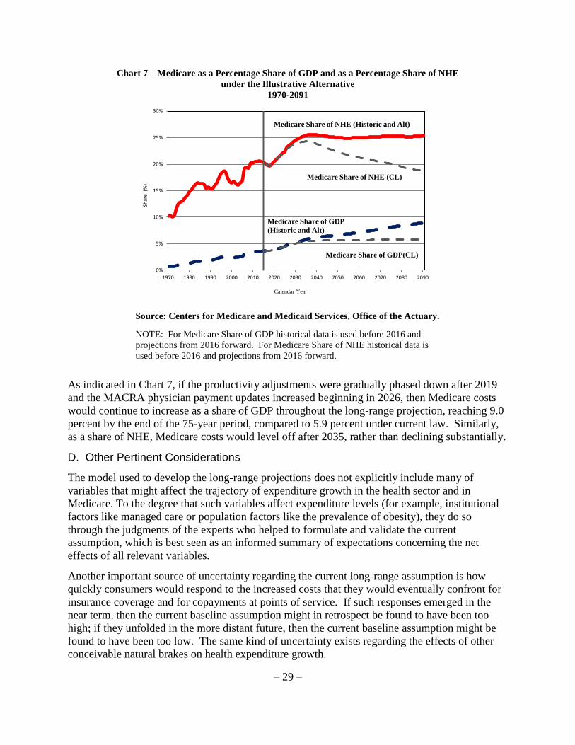
38 W.G. Manning, J.P. Newhouse, N. Duan et. al., “Health Insurance and the Demand for Medical Care: Evidence

from a Randomized Experiment,” American Economic Review, Volume 77(3), pages 251-277 (1987).

39 Amy Finkelstein, “The Aggregate Effects of Health Insurance: Evidence from the Introduction of Medicare,”

Quarterly Journal of Economics, Volume 122(1), pages 1-37 (2007).

– 26 –

pharmaceutical coverage plans. To some degree the perceived importance of cost-sharing may

continue to decline due to further expansion of the share of the population covered by public

programs like Medicaid. But OACT is persuaded that the role of cost sharing at the point of

service for Medicare beneficiaries as well as the financial burden of Part B and Part D premiums

will continue to increase, and absent policy interventions cost sharing effects in Medicare and in

the rest of the health sector would be even larger.

Cost-saving spillovers into Medicare from private sector initiatives that are focused on

rationalization of treatment around best practices are another foreseeable brake on excess cost

growth. The theory is that, as efficient methods of care become more widely diffused throughout

the health sector, such methods would be applied by health care practitioners to patients,

regardless of insurance plan. It is also possible that Medicare itself could contribute to this kind

of progress, resulting in cost savings that would spill over into private health plans as well. For

example, efforts are currently underway at CMS to test the effectiveness of better integration of

care through Accountable Care Organizations, patient-centered “medical homes,” shared savings

programs and capitated plans for dual Medicare-Medicaid beneficiaries, and other approaches.

Similarly, CMS is conducting demonstration programs for broader bundling of payments,

reductions in unnecessary hospital readmissions and hospital-acquired conditions, etc.

Innovations that are successful in reducing Medicare costs are very likely to be adopted in the

private sector as well.

It is also reasonable to expect that health care providers, under financial pressure from Medicare,

Medicaid, and the private sector alike, may adopt new technological innovations more prudently

than they have in the past. Drug and medical device manufacturers may focus greater attention

on developing cost-reducing technology in the future, more akin to what has traditionally

happened in other sectors of the economy.

These examples of “natural brakes” are expected to contribute to a slowdown over the long run

of excess cost growth even in the face of some foreseeable cost-increasing effects. For example,

persons who do not have or who choose to forgo a private supplemental Medicare insurance

policy may obtain extra coverage by enrolling in a Medicare Advantage (Medicare Part C) plan,

whose government-paid premiums and “rebates” (at least currently) often exceed average per

enrollee fee-for-service Medicare costs. To the degree that pharmaceutical coverage sponsored

by former employers of Medicare beneficiaries becomes less available or less comprehensive,

enrollment in the Medicare Part D plans may also grow, increasing total Medicare outlays. Also,

if a disenrollment trend emerged for Part B or Part D, it could be mitigated for some by increased

participation in Medicaid, including the “QMB,” “SLMB,” and “QI” options.

While there are natural brakes in the current health care system that are likely to slow excess

NHE and Medicare cost growth, the “out-of-sample” nature of the health expenditure projection

problem makes it especially difficult to project the magnitude and speed of a slowdown in the

rate of excess cost growth. Given the current state of knowledge and the recommendations of

distinguished panels of technical experts, OACT is satisfied that the current long-range

assumption, which incorporates a gradual slowing of cost growth from historical trends, is a

plausible and reasonable expression of trends likely to prevail under current law. A last attribute

of the current methodology is the assumption of the same cost slowdown to all parts of the U.S.

– 27 –

health sector.40 OACT is skeptical that a sustained divergence in cost growth rates between

Medicare and the rest of the U.S. health sector could prevail for long without the appearance of

access to care issues.

C. Current Law and Illustrative Alternative Medicare Projections

The Trustees Reports have presented materially-improved financial and actuarial statuses of the

Medicare program since the enactment of the ACA. The projected insolvency date of the HI

Trust Fund in the 2009 Trustees Report, the last report appearing under pre-ACA current law,

was 2017. In the 2017 Trustees report the insolvency date is 2029. Projected growth in the size

of the Medicare program as a share of total Gross Domestic Product (GDP) is substantially

smaller than under prior law. The 2009 Trustees Report projected Medicare's GDP share in year

75 as 11.4 percent whereas the 2017 Trustees Report projects Medicare's GDP share in year 75 at

5.9 percent under current law, with a major reason for this difference being the productivity

adjustments introduced by the ACA. Chart 6 displays the projected long-run expenditures of the

Medicare program as a share of GDP and as a share of aggregate national health expenditures,

based on the current law projections in the 2017 Medicare Trustees Report. As a share of GDP,

Medicare spending is projected to continue increasing until the late 2030s due to the combined

effects of excess cost growth and enrollment increases, though mainly due to the impacts of

increased enrollment. For the last 50 years of the projection the Medicare share of GDP is

relatively stable, reflecting slower enrollment growth and assumed per enrollee cost growth rate

that is near or below the per capita GDP growth rate. The convergence of per enrollee cost

growth to something near or below the rate of per capita GDP growth mainly occurs because the

growth in Medicare payment updates over this period are near the increases in the GDP deflator,

as required by the ACA. As a share of NHE, however, Medicare spending under current law is

projected to fall over the long-range as the assumed rate of per enrollee Medicare cost growth is

less than assumed for per capita NHE. Again the main reason for this pattern is the Medicare

payment updates, which are projected to increase at a slower rate than non-Medicare health price

updates (volume and intensity is assumed to grow similarly for Medicare and non-Medicare).

40 How excess cost growth for Medicare under the illustrative alternative scenario and other parts of the health sector

would slow is envisioned differently. For the privately insured, prices would be determined through the market

process whereas for the Medicare alternative scenario prices would be set through the update process for the

administrative payment systems.

– 28 –

Chart 6—Medicare as a Percentage Share of GDP and as a Percentage Share of NHE

under Current Law

1970-2091

Source: Centers for Medicare and Medicaid Services, Office of the Actuary.

NOTE: For Medicare Share of GDP historical data is used before 2016 and

projections from 2016 forward. For Medicare Share of NHE historical data is

used before 2016 and projections from 2016 forward.

As noted previously, there is substantial uncertainty concerning whether the ACA productivity

adjustments and the physician payment updates under MACRA could be sustained into the long-

run without affecting access to care by Medicare beneficiaries. Therefore, the Trustees also

report a long-range projection based upon an illustrative alternative scenario in which adherence

to the ACA and MACRA payment updates erode and cost-saving actions of the IPAB are

assumed to be overridden. Chart 7 displays projected long-run Medicare expenditures as a share

of GDP and NHE under the illustrative alternative scenario.

0%

5%

10%

15%

20%

25%

1970 1980 1990 2000 2010 2020 2030 2040 2050 2060 2070 2080 2090

Shar

e (%

)

Calendar Year

Medicare Share of NHE

Medicare Share of GDP

– 29 –

Chart 7—Medicare as a Percentage Share of GDP and as a Percentage Share of NHE

under the Illustrative Alternative

1970-2091

0%

5%

10%

15%

20%

25%

30%

1970 1980 1990 2000 2010 2020 2030 2040 2050 2060 2070 2080 2090

Shar

e (

%)

Calendar Year

Medicare Share of NHE (Historic and Alt)

Medicare Share of GDP

(Historic and Alt)

Medicare Share of NHE (CL)

Medicare Share of GDP(CL)

Source: Centers for Medicare and Medicaid Services, Office of the Actuary.

NOTE: For Medicare Share of GDP historical data is used before 2016 and

projections from 2016 forward. For Medicare Share of NHE historical data is

used before 2016 and projections from 2016 forward.

As indicated in Chart 7, if the productivity adjustments were gradually phased down after 2019

and the MACRA physician payment updates increased beginning in 2026, then Medicare costs

would continue to increase as a share of GDP throughout the long-range projection, reaching 9.0

percent by the end of the 75-year period, compared to 5.9 percent under current law. Similarly,

as a share of NHE, Medicare costs would level off after 2035, rather than declining substantially.

D. Other Pertinent Considerations

The model used to develop the long-range projections does not explicitly include many of

variables that might affect the trajectory of expenditure growth in the health sector and in

Medicare. To the degree that such variables affect expenditure levels (for example, institutional

factors like managed care or population factors like the prevalence of obesity), they do so

through the judgments of the experts who helped to formulate and validate the current

assumption, which is best seen as an informed summary of expectations concerning the net

effects of all relevant variables.

Another important source of uncertainty regarding the current long-range assumption is how

quickly consumers would respond to the increased costs that they would eventually confront for

insurance coverage and for copayments at points of service. If such responses emerged in the

near term, then the current baseline assumption might in retrospect be found to have been too

high; if they unfolded in the more distant future, then the current baseline assumption might be

found to have been too low. The same kind of uncertainty exists regarding the effects of other

conceivable natural brakes on health expenditure growth.

– 30 –

Actual long-range Medicare costs are virtually certain to differ from whatever is projected and,

as this consideration of sources of variability would suggest, perhaps to a very significant degree.

Such variation, however, is unlikely to be sufficient to alter the conclusion that the Medicare

program faces serious and enduring financial challenges that will become worse the longer that

they continue. OACT continues to engage in internal and external research projects aimed at

improving the foundations of the long-range health expenditure cost growth assumptions.

Conclusion

The Medicare Trustees have statutory responsibility to report on the long-term financial and

actuarial status of the Medicare program in the context of broader growth trends in the U.S.

health sector. To discharge this responsibility, long-range spending projections must be made

for both the overall health sector and Medicare, and those sets of projections must be

appropriately interrelated. For the 2017 Trustees Report, the FCG model was used to determine

the long-term growth trajectory of the U.S. health sector. The long-range Medicare cost growth

assumptions are computed as the increases in the volume and intensity of health care services per

person from the FCG model of total national health expenditures, adjusted by the expected

impact on volume and intensity from the ACA, together with the Medicare-specific provider

payment rate updates specified in current law, with further adjustments to incorporate

demographic effects. Continuing uncertainty concerning the feasibility of certain elements of

current law—the MACRA provision for physician payments and the permanent reductions in

most other Medicare payment updates by the increase in economy-wide productivity—has

prompted the Trustees to again provide an illustrative alternative projection whose growth

trajectory is the same as for the health sector as a whole.

The long-range cost growth assumptions have evolved through regular processes of expert

review, and improvements, refinements, and alternative approaches to the projection method

continue to be considered. In their present form, the long-range assumptions lead to Medicare

projections under current law and illustrative alternative scenarios that provide a sound basis for

evaluating long-range fiscal challenges for the Medicare program.

Stephen K. Heffler, M.B.A.

Director, National Health

Statistics Group

Sheila D. Smith, M.A.

Senior Economist

Todd G. Caldis, Ph.D, J.D.

Senior Economist

Gigi A. Cuckler, M.A., M.B.A.

Senior Economist

– 31 –

Appendix A: Factors Contributing to Growth (FCG) Model

The Office of the Actuary’s Factors Contributing to Growth (FCG) model is an accounting

framework that is used to track the historical contribution of factors that drive national health

expenditure growth and to develop projections of health care spending that are consistent with

the evolution of these factors. The model relies on a wide range of empirical research as the

basis for historical parameter estimates that reflect the sensitivity of health care spending growth

to changes in each of the factors. Where the projected path for these parameters is expected to

differ from historical patterns, the assumptions are adjusted to reflect the expected shift. These

parameters are applied to projected growth in macroeconomic and health-care-specific variables

to determine growth in national health spending over the long-term projection.

This appendix discusses the underlying structure of the FCG model. Next, it provides a detailed

discussion of the historical derivation of the key parameters in the model, and presents the

historical fit of the model from 1965-2015. Finally, this appendix discusses how the FCG model

is used as the framework for developing long-range projections of national health spending

growth that were used in the 2017 Trustees Report.

1. Factors Contributing to Growth (FCG) Model Structure

FCG model equation

There are five key factors that have been identified to influence growth in aggregate per capita

growth in national health expenditures:41

• demographics (the impact of distributional shifts across age and gender cohorts),

• changes in insurance coverage,

• relative medical price inflation,

• changes in aggregate real per capita income,

• a residual factor attributed primarily to the development and diffusion of new medical

technologies.42

These factors are used to develop the structure of the FCG model as shown in equation (1)

below:

(1) ht = at + y yt + i it + (1+p ) pt + dt

where each factor is expressed as a log difference (approximate growth rates) and all spending

series are in constant dollar terms based on the GDP deflator. Model variables are defined

below:

ht = constant dollar health spending per capita at time t

41 Sheila Smith, Joseph Newhouse, and Mark Freeland, “Income, Insurance, and Technology: Why Does Health

Spending Outpace Economic Growth?” Health Affairs, September/October 2009 28:1276-1284.

42 While there are a large number of potential factors that can be expected to influence health spending levels, most

cannot reasonably be assumed to influence growth rates over extended periods of time. A broad consensus holds

that technological change is the most critical factor that generates growth in health care spending sustained at rates

above what would be predicted based on other key factors contributing to growth.

– 32 –

at = residual factor (primarily attributed to spending on new medical technology)

yt = income at time t (GDP per capita)

it = average coinsurance rates at time t (out-of-pocket share of total health spending)

pt = relative medical price at time t (relative to GDP deflator)

dt = index of demographic contribution to health care spending at time t

Model parameters are defined as elasticities. Each elasticity represents an estimate of the

percentage change real per capita NHE that results from a one percentage point increase in that

model variable in question. These elasticities capture the sensitivity of health care spending

growth to changes from each of the causal factors. The elasticity associated with the index of

health care spending growth due to changes in the demographic composition of the population is

equal to one by construction (and is therefore not shown).

y = income elasticity

i = coinsurance elasticity

p = health care price elasticity

Note that growth in relative medical prices affects health spending in two ways in this model.

First, there is the direct impact of higher prices causing higher spending, other things being

equal. In addition, however, there is a partial offset to this effect as higher prices for medical

services tend to reduce demand somewhat, and this effect is reflected in the p· p term above

(where p is negative).

The contribution of medical technology to health care spending, primarily reflected as a in

equation (1), is defined as the incremental spending on treatment methods within the period

associated with adoption and diffusion of a new medical technology. This effect will reflect both

the relative utilization of the technology and its relative price in comparison with existing forms

of treatment. Effects on spending associated with technological change can be expected to

occur with a substantial lag, extending from the initial availability of the technology through its

diffusion to equilibrium (in the absence of changes in other variables).

The FCG model, as presented in equation (1), is a simple reduced-form picture that assumes that

the contribution of each of the factors to health spending growth is independent of all of the

others. The use of a reduced-form equation means that the model is not a behavioral equation.

Rather, it is effectively a summary of the relationship between health care spending growth and

the net effect of growth attributable to a range of factors on both the demand and supply side.

Equation (1) assumes that there will be no interaction effects among causal variables – the effect

of each factor is assumed to be independent of all others (i.e. ceteris paribus).

Where possible, the parameters in the model are estimated with other factors held constant.

However, there are cases where this is difficult to do. The most important of these is the

interaction effect between income and changing medical technology. Because this effect is so

critical, we attempt to explicitly incorporate it within the FCG Model, as discussed below.

To the extent that we are unable to fully control for interaction effects between the individual

factors contributing to growth, or where there are additional factors contributing to growth that are

not specified, the net impact of interactions and omissions on variation in health expenditure

growth will be incorporated in the contribution to growth from the residual term (a).

– 33 –

Income-technology interaction effect

In previous considerations of the factors driving health spending growth, it was typically

assumed as a simplification or approximation that the contribution to growth from technology

(attributed to the residual) was constant over the historical period. The contribution from medical

technology was assumed to be determined by technical rather than economic factors.

Technology was thus assumed to be exogenous to other factors in the model and its contribution

was assumed to be constant over the long-run projection period.43 However, the current version

of the FCG model acknowledges that economic as well as technical factors play a role in

determining the effects of technological change on health care spending growth. The

contribution of technological change is assumed to be a function of economic growth.

Both the direction and uptake of medical technology are responsive to ability and willingness to

pay for new forms of treatment. In other words, the effects of medical technology on health care

spending growth are conditional, not only on the state of medical knowledge, but also on public

and private budget constraints. Public and private budget constraints for spending on medical

care are determined by the total economic resources generated within the economy per person

(real per capita GDP). The implication of this interaction effect is that the contributions to

growth in health care spending attributable to growth in aggregate income and to advancing

medical technology are highly interrelated – to the point that it is difficult to estimate the

contribution from the two factors separately.

The FCG model shown in Equation (2) below is modified from the simpler version in Equation

(1) in one critical way to address this issue. Rather than treating the contribution of technology

to medical spending growth as an exogenous constant, we estimate the relationship between the

historical technology residual and real per capita GDP (as a proxy for average income). This

allows us to develop a projection of the technology residual that maintains consistency with the

historical relationship to the macroeconomic environment.44

(2) ht = at + y yt + iit + (1+p) pt + dt

where y is defined as the combined “income-technology elasticity”. It will be equal to y +

a(yt) from Equation (1), where a(yt) is variation in the residual that can be explained as a function

of real per capita GDP. The estimation of y is discussed below. The new residual at should

capture both changes in the state of medical knowledge that are independent of variation in

income, as well as the net effect of measurement issues and omissions. Equation (2) is used as

the FCG model in developing the year-by-year growth rates for the long-range projection for the

2017 Trustees Report.

43 Technical Review Panel on the Medicare Trustees Reports, Review of Assumptions and Methods of the Medicare

Trustees’ Financial Projections, Centers for Medicare and Medicaid Services (formerly Health Care Financing

Administration), December 2000.

44 There are other potentially important behavioral interaction effects that are not explicitly accounted for in the FCG

model. For example, a second important relationship is the effect of the extent and nature of insurance coverage on

the direction of medical research and the diffusion of new medical technology. Though this effect is widely

acknowledged, the current state of empirical research does not allow for this effect to be included in a way that is

defensibly grounded in historical data. See Edgar A. Peden and Mark S. Freeland, “Insurance Effects on U.S.

Medical Spending (1960-1993),” Health Economics, Volume 7, 1998: 671-687.

– 34 –

2. Estimation of FCG model parameters

Income-Technology Elasticity

Current OACT research on the income-technology elasticity implies that the combined

contribution of income and new medical technology accounts for an estimated 72 percent of

constant dollar per capita health spending growth over the period from 1980-2015.45 Thus, the

elasticity of real per capita health care spending with respect to income and technological change

is a critical parameter in the FCG Model.

A substantial empirical literature addresses the relationship between health care spending and

real per capita GDP.46 This relationship has long been recognized as a strong and consistent

empirical regularity in cross-country time-series data. Variations in real per capita GDP across

countries and time can predict a large part of the variation in real per capita health spending.

Higher income countries tend to introduce new technologies earlier and to encourage broad

diffusion into standards of medical practice.47 However, this literature does not treat technology

as an endogenous factor contributing to growth in health care spending. Rather, in a plurality of

studies that estimate an income elasticity, medical technology is assumed (implicitly or

explicitly) to be an exogenous variable.48 Many models used to estimate an income elasticity at

the aggregate level use pooled data across countries and time and commonly control for variation

across both countries and time by including fixed effects (dummy variables) for each country and

time period in the sample. Given that technology changes over time, but not across countries

within a single time period, its effect is assumed to be subsumed within the estimated fixed

effects by time period.

Equation (3) below shows a specification that is similar to those commonly used for the

estimation of the aggregate income elasticity. Aggregate national spending on health care is

represented as a function of real per capita GDP, and 2-way fixed effects (dummy variables) that

capture variation that is constant across all countries in the sample over time (time-period fixed

effects) and variation that is constant for each country in the sample across all time period

(country fixed effects).

45 This estimate is based on the mean estimate of the income-technology elasticity over the period 1980-2015,

obtained using an extrapolation of the income-technology elasticity.

46 Gerdtham U, Jönsson B. “International comparisons of health expenditures.” in: Culyer AJ, Newhouse JP, editors.

Handbook of Health Economics. Amsterdam (Netherlands): North-Holland; 2000: 11–53.

47 Moïse, Pierre, “The Heart of the Health Care System: Summary of the Ischaemic Heart Disease Part of the OECD

Ageing-Related Diseases Study,” in A Disease-based Comparison of Health Systems: What is Best and at What

Cost?, Organisation for Economic Co-operation and Development, 2003: 27-52.PAR

48 This choice largely reflects the difficulty of defining a variable that represents the state of medical technology;

while there have been attempts to develop a proxy for this concept (e.g. R&D, patents), these proxies cannot address

important issues such as the presence of long and variable lags in the relationship between R&D and health care

spending, or the fact that many important innovations are not patented (e.g. medical procedures).

– 35 –

(3)

ln (

ℎ𝑡

𝑝𝑡

𝑛𝑡) = 𝛼 + 𝛽 ln (

𝑦𝑡

𝑝𝑡

𝑛𝑡) + ∑ 𝑐𝑖 +

𝐼

𝑐=0

∑ 𝑧𝑡 + 휀𝑖𝑡

𝑇

𝑡=0

= constant term

ht = nominal health care spending converted to US dollars based on

purchasing power parities

yt = nominal GDP converted to US dollars based on purchasing power parities

pt = GDP deflator

nt = population

𝛽 = coefficient on real per capita income (income elasticity)

I = number of countries in pool

T = number of years in sample

z = fixed effect for each year t in the sample

c = fixed effect for each country i in the sample

εit = error term.

Current estimates of the income-technology elasticity are based on a specification that is similar

to Equation 3 but with the difference that time period fixed effects are excluded from the model

(see Equation 4 below). The income-technology elasticity incorporated in the FCG Model is

based on the estimation of Equation (4) based on pooled cross-country time-series OECD data

for 20 countries.49 Spending and income are defined in constant dollar per capita terms and

deflated based on the GDP deflator. Currency conversion to U.S. dollars is based on purchasing

power parities.50

(4)

ln (

ℎ𝑖𝑡

𝑝𝑡

𝑛𝑖𝑡) = 𝛼 + 𝛽′ ln (

𝑦𝑖𝑡

𝑝𝑡

𝑛𝑖𝑡) + ∑ 𝑐𝑖 + 휀𝑖𝑡

𝐼

𝑐=0

ht = nominal health care spending converted to US dollars based on purchasing power parities

yt= nominal GDP converted to US dollars based on purchasing power parities

pt = GDP deflator

nt = population

= constant term𝛽′= coefficient on real per capita income (income-technology elasticity)

I= number of countries in pool (20)

t = year

c= fixed effect for each country i in the sample

49 Countries in the sample include Australia, Austria, Belgium, Canada, Denmark, Finland, France, Germany,

Greece, Iceland, Japan, Netherlands, New Zealand, Norway, Portugal, Spain, Sweden, Switzerland, United

Kingdom, United States

50 Source: Organization for Economic Co-operation and Development (2014), "OECD Health Data", OECD Health

Statistics (database).

– 36 –

εit = error term.

The exclusion of fixed effects by time period in Equation (4) effectively means that a time trend

is acting as a proxy for technological change. Time-period fixed effects tend to be positively

correlated with growth in real per capita GDP. This implies that the coefficient 𝛽′ on real per

capita GDP based on Equation (4) is higher than the coefficient 𝛽 from Equation (3). The

coefficient 𝛽′ is conceptually comparable to the elasticity y from Equation (2). The difference

between 𝛽′ and 𝛽 is assumed to be attributable to a positive interaction effect between

technological change and income growth.

Change in the income-technology elasticity over time

The income-technology elasticity is assumed to change over the projection interval and the

historical rate of change over time is estimated empirically. The change in the elasticity in the

historical data is determined by estimating on the model specification in Equation (4) over a

series of rolling 21-year sample intervals (within the full data sample extending from 1970

through 2012).51 The model in Equation (4) was estimated for 21-year sample intervals, starting

with 1970-1990, and incrementing the start and end date of the sample by a single year through

the final sample interval of 1992-2012. The estimated elasticity based on each of these sample

intervals was attributed to the 11th year (the midpoint) of the 21-year sample, resulting in a time

series for the income-technology elasticity for the period from 1980 through 2002.

The results of this estimation show a systematic decline in the income-technology over the

period from 1970 through 2012. The rate at which the elasticity declines tends to slow down

over time. The time-series shown in Figure A.1 provides an estimate of the historical change in

the income-technology elasticity over the period 1980-2002. This time series is used as the basis

to evaluate the appropriate assumption for the income-technology elasticity over the 75-year

projection interval (currently extending from 2016 through 2091). This greatly strengthens the

empirical basis for the long-term assumption for this parameter. However, a substantial degree

of uncertainty continues to be associated with the projection, as the historical interval represented

by the series (1970-2012) is fairly short in comparison with the projection interval (75 years) and

the estimates remain at least somewhat sensitive to issues of data and sample selection.

51 An alternative method of estimating change in the income-technology elasticity (𝛽′)would be to include an

interaction term between 𝛽′and some function of a time trend. We chose to estimate the change in this parameter

based on rolling regression to avoid imposing a functional form on the path of change. This becomes relevant when

we consider the projection of the elasticity over the 75-year projection interval, as the difference between (for

example) a liner and a log-linear time trend implies a large difference in the long-term assumption.

– 37 –

Figure A.1. —Income-technology Elasticity Estimates, 1980-2002

1.35

1.40

1.45

1.50

1.55

1.60

1.65

1.70

1.75

1.80

1980 1985 1990 1995 2000

Relative medical price inflation

Data sources for medical prices are consistent with those used in the National Health

Expenditure Accounts (NHEA).52 The price measure for total personal health care spending is a

chain-weighted deflator based on relevant Producer Price Indexes (PPI) and Consumer Price

Indexes (CPI), with the weight for each index set equal to the share of personal health care

expenditures accounted for by that type of service.

The historical estimate of the aggregate price elasticity (−0.4) is based on the estimate in the

OACTS’s NHE Projections Model.53 This elasticity exceeds the out-of-pocket price elasticity of

−0.2 estimated based on the Rand Health Insurance Experiment (HIE). This higher price

elasticity at the aggregate level reflects the broader definition of the elasticity, which includes

price sensitivity at the market level in addition to the price effects for households in response to

variations in the effective out-of-pocket price that are the basis for the HIE elasticity. Additional

price sensitivity occurs at the point of purchase of private health insurance and in the process of

selective contracting by insurers acting as agents for consumers.

Insurance coverage

The effects of insurance are defined based on the aggregate average out-of-pocket share of health

expenditures. This definition is conceptually consistent with the elasticity based on the Rand

HIE (−0.2).54 The estimation of this insurance elasticity was primarily cross-sectional based on

variation in health care spending as a function of the generosity of insurance coverage across

52 See documentation of historical National Health Expenditures data, downloadable at

https://www.cms.gov/Research-Statistics-Data-and-Systems/Statistics-Trends-and-

Reports/NationalHealthExpendData/Downloads/DSM-15.pdf

53 Centers for Medicare and Medicaid Services. “Projections of national health expenditures: methodology and

model specification.” Available from: http://www.cms.gov/Research-Statistics-Data-and-Systems/Statistics-Trends-

and-Reports/NationalHealthExpendData/Downloads/ProjectionsMethodology.pdf.

54 Newhouse J, Health Insurance Experiment Group. Free for All? Lessons from the RAND Health Insurance

Experiment. Cambridge (MA): Harvard University Press; 1993.

– 38 –

households at a point in time, so this elasticity effectively holds technology constant. This

variable captures static effects of insurance coverage only. This includes the increased

utilization of current medical technologies in response to reduced out-of-pocket price.

However, this effect would exclude any dynamic effects of insurance coverage on the

development of new medical technologies. Dynamic interaction effects between insurance and

technology are in theory included in the residual (a). There is also the potential for three-way

interaction effects among the contributions of insurance with both income and technology effects

that cannot be separated out based on our estimation methods. This suggests that some part of

the dynamic effects of insurance coverage may also be captured in the income-technology

contribution.

Demographic change

The effects of shifts in the population across age and gender cohorts are estimated based on the

historical and projected population cohorts over time prepared by the SSA Office of the Chief

Actuary on behalf of the Board of Trustees, combined with a base-year distribution of

expenditures across age-gender groups. The application of base-year weights to projections of

population by age-gender cohorts produces an index of growth in health spending that will result

from shifts across these cohorts.55 This methodology assumes that the distribution of

expenditures does not change over time in response to changes in the distribution of population

across age-gender cohorts.

Model residual

The contribution to growth in real per capita NHE from the FCG Model residual a is extremely

volatile historically. We use a 15-year moving-average to smooth the time series so that we can

better evaluate the path of this contribution over time (Figure A.2. below)

Figure A.2. —FCG Model Residual with Fitted Trend Line, 1980-2015

-1.0%

-0.5%

0.0%

0.5%

1.0%

1.5%

2.0%

1980 1985 1990 1995 2000 2005 2010 2015

Residual (15 year moving average)

Fitted Trend Line

55 2017 Annual Report of the Boards of Trustees of the Federal Hospital Insurance and Federal Supplementary

Medical Insurance Trust Funds, https://www.cms.gov/Research-Statistics-Data-and-Systems/Statistics-Trends-and-

Reports/ReportsTrustFunds/Downloads/TR2017.pdf

– 39 –

Based on the smoothed time series, the contribution of the model residual follows a downward

trend over time, averaging about 0.6 percentage points for the most recent five years from 2010-

2015.

Historical parameter assumptions

Table A.1.—Historical Elasticities Based on the FCG model

Equation (2) variable Historical estimate

Income-technology elasticity y 1.5-1.7

Insurance elasticity* i −0.2

Relative medical price elasticity p −0.4

*Reflects the static impact of insurance coverage

Table A.1. shows the historical elasticity estimates that are used in equation (2) to explain a large

part of historical growth in health spending over the period from 1966 through 2015, as shown in

Figure A.3. below.56

Figure A.3.—Growth in Constant Dollar Per Capita NHE, 1966-2015

Actual vs. Predicted using FCG Model

0.0%

2.0%

4.0%

6.0%

8.0%

10.0%

12.0%

1966 1971 1976 1981 1986 1991 1996 2001 2006 2011

Constant-dollar per capita NHE

Predicted Growth based on FCG Model

*The predicted values as shown in Figure A.3. also control for a substantial lag in the relationship

between health spending growth and income growth, by incorporating a five-year moving average

of growth in real per capita GDP. Figure A.3. is not directly comparable with Figure A.2, because

data shown in Figure A.2. are based on a 15-year moving average, while data in Figure A.3. are

not.

56 The predicted increases in real per capita health expenditures (Figure A.3.) include the estimated contribution

from a combined income-technology effect, relative medical price inflation, insurance coverage, and demographic

change.

– 40 –

3. FCG long-range projections model

Projections of health spending growth using the FCG model should be consistent with historical

relationships between growth in health spending and the individual factors contributing to

growth. However, a simple extrapolation of the historical relationships over 1960-2015 implies

an increase in the health share of spending that would ultimately absorb all available economic

resources. In the long run, if the health share of consumption continues to rise along its historical

trajectory, economic theory suggests that consumer preferences will adjust to slow the rate of

increase in the health share of GDP. This predicted change in consumer preferences implies that

the parameters in the FCG model can be expected to change over time. Specifically, as health

accounts for a rising share of consumption, we can expect to see rising sensitivity to relative

medical prices (as represented by the price elasticity), and a declining tendency to further

increase consumption of health care out of income at the margin (as represented by the income-

technology elasticity).

In the discussion below we present the FCG parameter assumptions over the projection period,

the exogenous parameter assumptions used to develop the FCG projections, and the results from

the FCG model that were used in the 2017 Trustees Report.

FCG Parameter Assumptions

The elasticity assumptions in the FCG model determine the sensitivity of national health care

expenditures to changes in each factor for the projection in the long-term (defined here as years

25 through 75 of the 75-year projection). As described above, economic theory suggests that as

the health share of consumption rises substantially over the long-term, the elasticities that

represent consumer preferences can be expected to change (see Table A.2. below). Specifically,

we can expect consumers to become increasingly sensitive to the relative price of goods that

account for a growing share of total consumption (implying a rising magnitude in the price

elasticity). We can also expect to see a decline in the income-technology elasticity over time.

An income-technology elasticity greater than one means that health spending will grow faster

than GDP, in the absence of a change in other factors (such as price). Though the historical

income-technology elasticity is estimated to be well above one, we can expect this parameter to

decline to one in a long-term equilibrium state so that non-health consumption is not crowded

out by the continued rise in the health share.

Table A.2. below provides a summary of the key elasticity assumptions used for the FCG model

in generating the growth in NHE applied in the 2017 Trustees Report.

Table A.2.—Elasticity Assumptions for FCG model: 2041-2091

Income-technology

elasticity (y )

Insurance

Elasticity (i )

Price elasticity

(p )

1.26 → 1.09 −0.2 −0.51 → −0.59

– 41 –

Income-technology elasticity assumption

To develop this assumption, we estimated the historical change in the elasticity empirically based

on cross-country time-series data from the OECD.57 This series was then projected forward over

the 75-year projection interval.

The estimated historical time series for the income-technology elasticity was projected based on

fitting the historical time series of the income-technology elasticity estimates (from the rolling

21-year regressions) as a function of the natural log of a time trend as shown in Equation (5)

below.58

(5) 𝛽𝑡=𝛾+𝛿′ln(𝑇REND(𝑏))+휀𝑡

TREND(b) = time trend such that TREND(b)=1, TREND(b+n) = 1+n, for n=1….30

b = base year for time trend

𝛽𝑡 = Income-technology elasticity estimates based on the rolling regressions with midpoint t

t = year representing the sample midpoint from the rolling regressions (t=1980….2002)

γ = constant term

δ = coefficient on trend variable

As the base year of the trend increases, the log of the trend increases in curvature. The

coefficient was estimated based on this specification, which was selected by varying the base

year of the time trend so as to maximize the adjusted R-Squared for equation (5).

The resulting actual versus predicted values for the income-technology elasticity, with the

projection based on this model are shown below in Figure A.4.

57 Source: Organization for Economic Co-operation and Development (2014), "OECD Health Data", OECD Health

Statistics (database).

58 The use of a log-based time trend was selected following evaluation of alternative functional forms. The choice

of a log-form implies that the rate of change in the income-technology elasticity will tend to slow over time. This

pattern of change was consistent with the estimated historical time-series for the income-elasticity, and also tended

to produce a more reasonable projection that levels out near a value of 1.0 in the long-term. In comparison, a linear

time trend implies a constant rate of decline that ultimately reaches zero unreasonably fast (much sooner than the

end of the 75 year projection).

– 42 –

Figure A.4.— Income-Technology Elasticity Estimates:

Historical Estimates and Projections for 2017 Trustees Report

0.9

1.1

1.3

1.5

1.7

1.9

Income-technology elasticity Predicted values

Fitted values,

1980-2002Projection 2016-2091

Price elasticity assumptions

The price elasticity of demand for health care (p) is inelastic over the history (estimated at -0.4),

meaning that a one percentage point increase in medical prices relative to economy-wide prices

is associated with a -0.4 percentage point reduction in real health care consumption. This also

implies that the net impact of medical prices rising faster than economy-wide inflation on

nominal health care spending growth is positive. Over the long-term, medical prices are

projected to continue to grow faster than economy-wide prices, although the differential is

expected to be smaller than has been the case historically. However, as discussed earlier, the

magnitude of the price elasticity is expected to increase (in absolute value) as the share of

consumption allocated to health care rises over time.59

The rationale for the increase in consumer price sensitivity (or magnitude of the price elasticity)

implies that the price elasticity will be a function of the health share of GDP. This relationship

is derived from the Slutsky Equation (see Box 1). Within the FCG Model, this means that the

price elasticity is endogenously determined, since the health share of GDP is a function of all of

59 Silberberg, Eugene, The Structure of Economics: A Mathematical Analysis, McGraw-Hill, 2000.

– 43 –

the parameter assumption in Equation (2). The effects of this endogeneity have been explicitly

incorporated in the model.60

The resulting projection of the price elasticity is assumed to decline from the historical estimate

of −0.4 to −0.5 by year 25 of the projection, and to then decline further to −0.6 by year 75 of the

projection.

Box 1: Projecting the price elasticity of demand for health care as the health share of

consumption rises

The Slutsky equation (in elasticity form) is an identity that decomposes the price

elasticity into two components: a pure substitution effect and an income effect. The pure

substitution effect is not observed—it is the change in demand in response to a change in

the relative price of health care holding utility constant. The income effect occurs

because a rise in price implies a lower income. That is, the greater the share of health

care out of total consumption, and the higher the income elasticity, the larger will be the

income component of the price effect:

p = c

p - sh y

where p is the observed price elasticity, c

p is the compensated price elasticty (or pure

substitution effect), sh is the health spending share of total consumption, and y is the

income-technology elasticity.

Given assumptions of price and income elasticities and historical data on the health share

of consumption, we can back out the unobserved pure substitution effect (compensated

price elasticity). If in 2013 the observed price elasticity is −0.4, the income-technology

elasticity (including interaction effects) is 1.4, and the health share of GDP is 17 percent,

then the compensated price elasticity is estimated at −0.2 (calculated as −0.4 + 0.17×1.4).

We assume that the compensated elasticity remains constant at −0.2 over time as the pure

substitution effect is not affected as the health share of consumption changes. We can

combine this constant with preliminary projections for the health share of consumption

and the assumed income-technology elasticity over time to impute the rise in the total

price elasticity that is consistent with the rising share of health care spending.

Note that the health share of GDP will be influenced by the projected price elasticity.

This means that the system will be simultaneous by nature. However, we can approach

an answer that is fairly stable by iterating between the projections based on the FCG

model and the relationship between elasticities in the Slutsky equation. The resulting

estimate for the price elasticity (p) in year 75 is −0.6 (which is determined by −0.6 =

−0.2 − 0.35×1.1), as shown in table A.2.61

60 The endogeneity of the price elasticity and the health share of GDP effectively require a simultaneous model

solution. We approximate this result by solving the model iteratively for the price elasticity and the health share,

and then resolving the model until both concepts converge to an internally consistent solution.

61 Estimate is calculated using the health share of GDP under the Illustrative Alternative Scenario.

– 44 –

FCG Model Residual Assumptions

The residual expenditure growth (at ) estimated from the historical predictions of the FCG model

in equation (2) is highly volatile, with a positive, declining trend over the 1980-2015 period.

The historical trend through the most recent data exhibits a declining trend over 1980-2015

(Figure A-2 above). An extrapolation of historical trend implies that the residual can be

expected to approach zero over the period of the short to medium term projection (2016-2041).

Consistent with past assumption, we assume that this residual is equal to zero over the long-term

projection period from 2041-2091.

Future research efforts will be focused evaluating the specification of the FCG Model in

Equation (3) to determine if the specification of the model can be improved to produce a smaller

residual, and on quantifying the uncertainty associated with projecting the historical trend in the

residual.

Exogenous Assumptions

The key economic assumptions for per capita GDP and the GDP deflator are from the

intermediate set of assumptions underlying the 2017 Social Security and Medicare Trustees

Reports. The relative medical price inflation is determined based on long-range assumptions

regarding growth in medical input prices and available evidence on achievable resource-based

health sector productivity growth. As described in the main text of this memorandum, medical

input prices are assumed to grow at roughly 3.4 percent per year. Overall resource-based health

sector productivity is assumed to grow at 0.4 percent per year by assuming hospital and

physician productivity will grow at published historical rates (0.4 percent and 1.1 percent,

respectively),62 while all other provider categories, such as skilled nursing facilities, home health

agencies, hospices, diagnostic laboratories, dialysis centers, ambulance companies, etc., will

grow at zero, on average. Combining these assumptions produces a medical output price

increase of 3.0 percent per year, which is 0.8 percentage point faster than the GDP deflator.

Thus, the FCG model uses a relative medical price inflation assumption of 0.8 percent per year,

equivalent to the historical average growth in the deflator for personal health care spending,

relative to the GDP deflator, over the period from 1990-2015.63

Finally, it is assumed in the FCG model that the out-of-pocket share of national health

expenditures remains unchanged over the projection period. This assumption reflects, in part,

that the average cost sharing associated with the Medicare benefit is likely to remain stable over

the long-range projection period under current law, including consideration of the effects of

supplemental coverage through private Medigap policies, Medicare Advantage plans, employer-

sponsored retiree health plans, and Medicaid.

62Information on updated estimates of hospital productivity is available at https://www.cms.gov/Research-Statistics-

Data-and-Systems/Statistics-Trends-and-Reports/ReportsTrustFunds/Downloads/ProductivityMemo2016.pdf. Estimates of physician productivity are available here: Charles Fisher, “Multifactor productivity in physicians’

offices: An exploratory analysis,” Health Care Financing Review, Volume: 29, Issue: 2, 2008. p. 15-32.

63 CMS, Office of the Actuary, National Health Expenditure Accounts: http://www.cms.gov/Research-Statistics-

Data-and-Systems/Statistics-Trends-and-Reports/NationalHealthExpendData/

NationalHealthAccountsHistorical.html.

– 45 –

Results

The FCG model output was used to determine the year-by-year growth rates for overall national

health spending and volume and intensity in the 2017 Trustees Report. Figure A.5. below shows

the excess cost growth rates from the FCG model based on the methods and assumptions

described above. As noted in the main body of this memorandum, the volume and intensity

growth rates from the FCG model were used with the Medicare-specific payment rate updates

under current law and anticipated impacts on volume and intensity from the ACA to obtain the

projected increases in Medicare expenditures per beneficiary by type of service.

Figure A.5.—Long-Range NHE Excess Cost Growth*

based on the FCG Model

Source: Centers for Medicare & Medicaid Services, Office of the Actuary.

*Excess Cost Growth is defined as growth in per capita, age-gender adjusted

health spending less growth per capita GDP.

0.00%

0.25%

0.50%

0.75%

1.00%

1.25%

1.50%

1.75%

2.00%

2041 2046 2051 2056 2061 2066 2071 2076 2081 2086 2091

Exce

ss c

ost

Gro

wth

*

Year of 75-year Projection Period

2017 TR NHE ECG Growth2016 TR NHE ECG Growth