arX

iv:a

stro

-ph/

0605

621v

2 2

1 A

ug 2

006

Mass functions in coupled Dark Energy models.

Roberto Mainini, Silvio Bonometto

Department of Physics G. Occhialini – Milano–Bicocca University,

Piazza della Scienza 3, 20126 Milano, Italy and

I.N.F.N., Sezione di Milano

(Dated: October 1, 2018)

Abstract

We evaluate the mass function of virialized halos, by using Press & Schechter (PS) and/or Steth

& Tormen (ST) expressions, for cosmologies where Dark Energy (DE) is due to a scalar self–

interacting field, coupled with Dark Matter (DM). We keep to coupled DE (cDE) models known to

fit linear observables. To implement the PS–ST approach, we start from reviewing and extending

the results of a previous work on the growth of a spherical top–hat fluctuation in cDE models,

confirming their most intriguing astrophysical feature, i.e. a significant baryon–DM segregation,

occurring well before the onset of any hydrodynamical effect. Accordingly, the predicted mass

function depends on how halo masses are measured. For any option, however, the coupling causes

a distortion of the mass function, still at z = 0. Furthermore, the z–dependence of cDE mass

functions is mostly displaced, in respect to ΛCDM, in the opposite way of uncoupled dynamical

DE. This is an aspect of the basic underlying result, that even a little DM–DE coupling induces

relevant modifications in the non–linear evolution. Therefore, without causing great shifts in linear

astrophysical observables, the DM–baryon segregation induced by the coupling can have an impact

on a number of cosmological problems, e.g., galaxy satellite abundance, spiral disk formation,

apparent baryon shortage, entropy input in clusters, etc..

PACS numbers: 98.80.-k, 98.65.-r

1

INTRODUCTION

A first evidence of Dark Energy (DE) came from the Hubble diagram of SNIa, showing an

accelerated cosmic expansion, but a flat cosmology with Ωm ≃ 0.25, h ≃ 0.73 and Ωb ≃ 0.042

is now required by CMB and LSS observations and this implies that the gap between Ωm

and unity is to be filled by a smooth non–particle component, whose nature is one of the

main puzzles of cosmology. (Ωm,b: matter, baryon density parameters; h: Hubble parameter

in units of 100 km/s/Mpc; CMB: cosmic microwave background; LSS: large scale structure.)

If DE is a false vacuum, its pressure/density ratio w = pDE/ρDE is strictly -1. This option,

however, implies a severe fine tuning at the end of the electroweak transition. Otherwise

DE could be a scalar field φ, self–interacting through a potential V (φ) [1], [2], so that

ρDE = ρk,DE + ρp,DE ≡ φ2/2a2 + V (φ), pDE = ρk,DE − ρp,DE , (1)

provided that dynamical equations yield ρk,DE/V ≪ 1/2, so that −1/3 ≫ w > −1. Here

ds2 = a2(τ)(−dτ 2 + dxidxi) , (i = 1, .., 3) (2)

is the background metric and dots indicate differentiation with respect to τ (conformal time).

This kind of DE is dubbed dynamical DE (dDE) or quintessence; the w ratio then exhibits a

time dependence set by the shape of V (φ). Much work has been done on dDE (see, e.g., [3]

and references therein), also aiming at restricting the range of acceptable w(τ)’s, so gaining

an observational insight onto the physics responsible for the potential V (φ).

As a matter of fact, the dark cosmic components are one of the most compelling ev-

idences of physics beyond the standard model of elementary interactions and, while lab

experiments safely exclude non–gravitational baryon–DE interactions, DM–DE interactions

are constrained just by cosmological observations. In turn, DM–DE interactions could ease

the cosmic coincidence problem [4], i.e. that DM and DE densities, differing by orders of

magnitude since ever, approach one another at today’s eve.

In a number of papers, constraints on coupling, coming from CMB and LSS observations,

were discussed [4, 5, 6]. This note aims at formulating predictions on the mass function of

bound systems in coupled DE (cDE) cosmologies, by using Sheth & Tormen [9] expressions,

known to improve the original Press & Schechter [8] approach. Our final scope amounts to

finding stronger constraints on DM–DE coupling, arising from a comparison of observational

2

data with our predictions, opening a basic window on the nature and origin of these very

components. Our analysis will be restricted to SUGRA [10] and RP (Ratra–Peebles) [2]

potentials

SUGRA V (φ) = (Λα+4/φα) exp(4πφ2/m2p)

RP V (φ) = (Λα+4/φα) (3)

(mp = G−1/2: Planck mass), admitting tracker solutions. This will however enable us to

focus on precise peculiarities, not caused by the shape of V (φ) but by the coupling itself.

Let us also remind that, once the DE density parameter ΩDE is assigned, either α or the

energy scale Λ, in the potentials (3), can still be freely chosen. In this paper we show results

for Λ = 102GeV; minor quantitative shifts occur when varying log10(Λ/GeV) in the 1–4

range. The RP potential will be mostly considered to test the effects of varying DE nature.

The effects of coupling can be seen in the background equations for DE and DM, reading

φ+ 2(a/a)φ+ a2V,φ =√

16πG/3βa2ρc , ρc + 3(a/a)ρc = −√

16πG/3βρcφ ; (4)

here β sets the coupling strength and, all through this paper, we take it constant (and, in

particular, independent of φ; a different case, which can be physically significant and may

deserve a separate treatment [7]) with values β = 0.05 or 0.20 . In previous work this was

considered a small strength. CMB data set a limit β <∼ 0.6; a stronger constraint found

by [6], by studying cluster profiles in n–body simulations, applies to RP potentials only.

On the contrary, even for the smaller coupling we considered, we find significant devia-

tions from uncoupled models in non–linear observables. Such deviations exhibit intriguing

features, suggesting possible ways out from a number of astrophysical problems, while the

small coupling strength scarcely affects linear observables.

As far as the other model parameters are concerned, we take density parameters Ωm =

0.25, Ωb = 0.042, Ωc = 0.208 and h = 0.73. This choice approaches the best fit of a ΛCDM

model to available data. A best fit to cDE models will certainly yield slightly different

parameters, but this implies just minor shifts in our quantitative findings.

BARYON AND DARK MATTER DYNAMICS

The essential novel feature induced by DM–DE coupling in non–linear structures is

baryon–DM segregation. This was shown in [11] (paper I, hereafter). The reason why segre-

3

gation occurs can be easily illustrated by considering, aside of the eq. (4), ruling background

dynamics, the couple of equations telling us how the baryon (DM) density fluctuations δb

(δc) and velocity fields

θc,b = ik · vc,b

H . (5)

depend on τ (H = a/a; k: wavenumber of the fluctuation considered). They read

δc′′ = −δc ′(1 +

H′

H − 2βX) +3

2(1 +

4

3β2)Ωcδc +

3

2Ωbδb,

δb′′ = −δb ′(1 +

H′

H ) +3

2(Ωcδc + Ωbδb), (6)

θc′ = −θc(1 +

H′

H − 2βX)− 3

2(1 +

4

3β2)Ωcδc −

3

2Ωbδb, ,

θb′ = −θb(1 +

H′

H )− 3

2(Ωcδc + Ωbδb) . (7)

Here ′ yields differentiation with respect to α = ln a and

X =√

4π/3 φ/(mpH) . (8)

Both eqs. (4) and eqs. (6)–(7) show that, as soon as β 6= 0, baryons and DM have differ-

ent dynamics. Neglecting radiation and any hydrodynamical effects, baryons move along

geodesics. On the contrary, DM particles feel also non–gravitational forces and, as it hap-

pens in the presence of any non–gravitational interaction, do not follow geodesics. This is

why baryon–DM segregation occurs.

Starting from eqs. (6)–(7), the evolution of linear fluctuations in cDE cosmologies was

studied by [4]. Here we shall put ourselves into a different physical context, by lifting

the restriction δc,b ≪ 1, but considering just cases when a full relativistic treatment is

unessential. Then, dealing with scales well below horizon and with non–relativistic particles,

the long–range force carried by the DE field φ can be described through corrections to

newtonian gravity. They amount to assuming:

(i) DM particle masses to vary, so that

Mc(τ) =Mc(τi) exp[−C(φ− φi)]. (9)

(ii) The gravitational constant between DM particles to become G∗ = γG.

Here

C =√

16πG/3 β , γ = 1 + 4β2/3 (10)

4

A proof is given in Appendix A, following [12] and [6].

A newtonian treatment is suitable to study the growth of spherical top–hat fluctuations

in the DM and baryon components and to show how their segregation occurs in the relevant

physical cases. In fact, non–linearity starts well after matter–radiation decoupling and the

top scales to be considered, galaxy cluster scales, lay well below the horizon.

The evolution of fluctuations in this regime was debated in paper I. Here we shall use

its results to understand the shaping of mass functions. We therefore start from reviewing

them and complementing them with new quantitative outputs.

SPHERICAL TOP–HAT EVOLUTION

Although in all cosmologies, apart sCDM, the system of equations ruling the spherical

growth requires a numerical solution, in cDE models the numerical approach is far more

essential. In fact, in all cases apart cDE, the only variable describing a top–hat fluctuation is

its radius R. It is assumed to expand, initially, at the same rate of the scale factor a, obeying

an equation similar to the scale factor in a closed model. The greater density inside the top

hat slows then down the increase rates of R in respect to a, so that the inner density ρ(< R),

although decreasing, becomes greater and greater than the average density ρ. Eventually,

at a time tta, when the density contrast ∆ = ρ(< R)/ρ attains a suitable value χ, R stops

and starts decreasing. The equation it obeys would then cause R to vanish within a finite

time tc. In sCDM cosmologies, χ = (3π/4)2 and tc/tta = 2. In other non–cDE cosmologies,

χ and the ratio tc/tta take just slightly different values.

After tta, however, the very density inside R is increasing, so that, in any realistic fluc-

tuation, unless radiation disposes the heat produced by the p dV work, virial equilibrium is

attained and the collapse essentially stops when the fluctuation radius is Rv. In a sCDM

cosmology this occurs for Rv/Rta = 1/2. Taking onto account the symultaneous growth of

a, the virial density contrast is then ∆v = 32χ ≃ 180. In other cosmologies the Rv/Rta

ratio is slightly different from 1/2 and ∆v is mostly above 100, but, in most cases, signifi-

cantly below 180. A usual assumption is that the time when the system is stabilized into

a virialized configuration coincides with tc. Let us also remind that while, in sCDM, ∆v is

independent from tc, this is no longer true in all models where the density ratio between DE

and material components depends on time.

5

Quantitative results for the spherically symmetric growth in ΛCDM models were given by

[13]; their extension to models with uncoupled dDE is due to [14, 15]. In these cosmologies,

the simple system of equations yielding spherical evolution requires a numerical solution.

Let us now consider the same problem in the cDE case. This problem had been considered

in [16], but its approximated treatment did not allow the authors to focus the main physical

effects. Following [11], let us outline, first of all, that linear fluctuations in baryons and DM

are already different [12] and have a ratio

δbδc

≃ 3Ωc

3γ Ωc + 4β Xµ. (11)

Here X is given in eq. (8), γ is given in eq. (10); µ = (δc,b/δc,b)/H. When considering a

spherical top–hat fluctuation, whose initial radius RTH,i = Rb = Rc, eq. (11) sets the initial

ratio between DM and baryon fluctuation amplitudes.

Initial conditions are set so that bothRb andRc initially grow as the scale factor. However,

because of the different interaction strength, as soon as non–linear effects become significant,

Rb starts exceeding Rc. Hence, a part of the baryons initially within RTH,i leak out from Rc,

so that DM does not feel the gravity of all baryons, while baryons above Rc feel the gravity

also of initially unperturbed DM layers. As a consequence, above Rc, the baryon component

deviates from a top–hat geometry, while a secondary perturbation in DM arises also above

Rc itself.

After reaching maximum expansion, contraction will also start at different times for

different components and layers. Then, inner layers will approach virialization before outer

layers, whose later fall–out shall however perturb their virial equilibrium. This already

outlines that the onset of virial equilibrium is a complex process.

Furthermore, when the external baryon layers fall–out onto the virialized core, richer of

DM, they are accompanied by DM materials originally outside the top–hat, perturbed by

baryon over–expansion.

The time when the greatest amount of materials, originally belonging to the fluctuation,

are in virial equilibrium occurs when the DM top–hat has virialized, together with the

baryon fraction still below Rc. A large deal of baryonic materials are then still falling out.

But, when they will accrete onto the DM–richer core, they will not be alone, carrying with

them originally alien materials. There will be no discontinuity in the fall–out process when

all original baryons are back. The infall of outer materials just attains then a steady rate.

6

In order to follow the dynamical evolution of a systems where each layer feels a different

and substance–dependent force, a set of concentric shells, granting a sufficient radial reso-

lution, needs to be considered. In the next section we shall provide the equations of motion

for Lagrangian shell radii and review the whole expansion and recontraction dynamics.

TIME EVOLUTION OF CONCENTRIC SHELLS

The spherical growth

Dynamical equations can be written by using comoving radii bn = Rnb /a (cn = Rn

c /a) for

the n–th baryon (DM) shell. Let Mnb,c be the masses of the n–th layer, Mn

b,c be the masses in

the same layer in the absence of perturbations, and δMnb,c =Mn

b,c−Mnb,c be the mass excesses

for the n–th layer. Baryon shells keep a constant mass in the whole process, while

Mnc (τ) =Mn

c (τin) exp−C[φ(τ)− φ(τin)] , (12)

according to eq. (9). Similarly, let ∆Mb,c(< r) = Mb,c(< r)− Mb.c(< r) be the mass excess

within the physical radius R = ar and let then be

∆Mnb = ∆Mb(< bn) + ∆Mc(< bn) , ∆Mn

c = ∆Mb(< cn) + γ∆Mc(< cn) , (13)

including a correction aimed to take into account, besides of the mass variation (eq. 12),

also that G∗ 6= G in DM–DM interactions.

A systematic discrepancy will arise between bn and cn and will require taking into account

only the fraction of the last shell below the radius considered. In paper I it is shown that

the shell dynamics can then be described through the equations

cn = −(

a

a− Cφ

)

cn −G∆Mn

c

ac2n, bn = − a

abn −G

∆Mnb

ab2n, (14)

to be integrated together with the first of eqs. (4) and the Friedman equation.

Until bn ∼ cn, it is ∆Mnb < ∆Mn

c , for any β > 0. Hence, the gravitational push felt by

DM layers is stronger. The extra term Cφcn adds to this push. In fact, the comoving variable

cn has however a negative derivative (see the lower panels in Figure 1). As a consequence,

cn decreases more rapidly than bn, so that the n–th baryon radius may gradually exceed the

(n+ 1)–th DM shell, etc. . As a consequence, the sign of ∆Mnb −∆Mn

c can even invert and

7

DM bar

DM bar

FIG. 1: Evolution of a sample of baryon and DM layer radii, extending up to the top–hat radius;

upper (lower) panels describe physical (comoving) radii. In all plots the leaking out of the upper

baryon layer is clearly visible.

one can evaluate for which value of φ − φi this occurs. Once φ(τ) is known, also the time

when this occurs can be found. Until then, however, DM fluctuations expand more slowly

and mostly reach their turn–around point earlier, while baryons gradually leak out from the

fluctuation bulk.

The whole behavior is visible in the Figure 1, for samples of Rc,b and c–b (the ordinate

label x stands for either c or b). The greatest radii shown are the baryon top–hat radii.

Solid (dotted) lines yield the a dependence for DM (baryon) shell radii. The actual number

of radii Rnb,c used in the equations depend on the precision wanted; radii do not need to be

equi–spaced. To our aims (a 0.1% precision), ∼ 1000 radii were sufficient. If more precision

is needed, it can be easily achieved at the expenses of using a greater computer time. With

a single processor 1.5 Gflops PC, our optimized program takes ∼ 60 minutes to run a single

case, with ∼ 1000 radii.

8

DM bar

FIG. 2: Density profiles at different a values for a cDE model with β = 0.05. Solid (dotted) lines

refer to DM (baryons). Notice the progressive deformation of the baryon profile (dotted lines) in

respect of the DM profile (solid line).

DM bar

FIG. 3: Density profiles at different a values for β = 0.2 model. The deformation of the baryon

profile (dotted lines) in respect of the DM profile (solid line) is stronger than in the previous Figure.

9

The full collapse shown in Figure 1 is not expected in any physical case, as the Rn

decrease stops when virialization is attained. Figs. 2, 3 therefore assume that the spherical

growth stops when all DM originally in the top–hat, and the baryons kept inside it, virialize.

This figure describes the gradual deformation of the top–hat profile. Already at a = 0.2,

well before the turn–around, the slope of the top–hat boundary, for baryons, is no longer

vertical. At a = 0.6 (approximately turn–around), not only the baryon boundary is bent,

but a similar effect is visible also for DM. The effect is even more pronounced at avir ≃ 0.92.

Figures similar to the upper plots in Fig. 1 and to Figs. 2, 3 were already shown in paper I,

although for different model parameters.

The increased density of DM shells outside the top–hat is relevant, here, because it

fastens the recollapse of outer baryons. In turn, the enhanced baryon density, outside from

DM top–hat, modifies the dynamics of external DM layers, as well.

The most significant physical effect, however, is the outflow of baryon layers from the DM

top–hat. The outflown baryon fraction increases with a. For a ∼ 0.92, i.e. when DM and

inner baryons have attained their virialization radius, the fraction of baryons which have

leaked out from the fluctuation is so large as ∼ 10%, even for β = 0.05; it reaches ∼ 40%

for β = 0.2 . These values increase by an additional 10% in the RP case.

Virialization

In Figures 2 and ?? we assumed the present time to coincide with virialization for all

DM inside the top–hat fluctuation and all baryons kept inside it, excluding therefore a large

deal of baryons, either 10 or 40%, initially inside the top–hat, but leaking out during the

fluctuation growth.

It must also be outlined that much care ought to be taken to define the virialization

condition, for materials within any radius R, reading

2 T (R) = RdU(R)/dR , (15)

by summing up DM and baryon kinetic energies

Tc(R) = 2π∫ R

0dr r2ρc(r) r

2 , Tb(R) = 2π∫ R

0dr r2ρb(r) r

2 (16)

and taking into account that, during the whole fluctuation evolution, potential energies

include three terms, due to self–interaction, mutual interaction, interaction with the DE

10

field. More in detail, for DM and baryons, we have

Uc(R) = Ucc(R) + Ucb(R) + Uc,DE(R) = 4π∫ R

0dr r2 ρc(r) [Ψc(r) + Ψb(r) + ΨDE(r)] , (17)

Ub(R) = Ubb(R) + Ubc(R) + Ub,DE(R) = 4π∫ R

0dr r2 ρb(r) [Ψb(r) + Ψc(r) + ΨDE(r)] , (18)

respectively. While

Ψb(r) = −4π

3Gρb(r)r

2 , ΨDE(r) = −4π

3GρDE(r)r

2 , (19)

in both expressions, a subtle difference exists for Ψc. In Ub we have simply

Ψc(r) = −4π

3Gρc(r)r

2 , (20)

as for the other components, but this expression is different in Uc, where it reads

Ψc(r) = −4π

3γG[ρc − ρc(r)] +Gρcr2 , (21)

ρc being the background DM density. The different dynamical effect of background and DM

fluctuation arises from the different ways how its interaction with DE is treated. Energy

exchanges between DM and DE, for the background, are accounted for by the r.h.s. terms

in eqs. (4). In this case no newtonian approximation was possible and was made. For DM

fluctuation, instead, the effects of DM–DE exchanges are described by a correction to the

gravitational constant G, becoming G∗ = γG, which adds to the dependence of DM density

on φ. This ought to be taken into account in the fluctuation evolution, as is done in eq. (21).

The above expressions hold for any R. However, if R coincides with DM top–hat (or is

smaller than it), the densities ρb,c,DE do not depend on r. Densities depend on r if one aims

to take somehow into account the shells where baryons, initially belonging to the top–hat,

have flown. In the former case, the integrals (17), (18) and (16) can be easily performed

and yield

Uc(R) = (3/5)G[Mc(Mb + Mc) + γMc∆Mb]/R− (4π/5)McρDER2 (22)

Ub(R) = −(3/5)G[Mb(Mb +Mc)]/R− (4π/5)MbρDER2 (23)

Tc(R) = (3/10) McR2 (24)

11

where the relation r/r = R/R is used to calculate Tc(R). Note that this relation is not

valid for Tb(R) because different baryon layers have different growth rates. Kinetic energy

for baryons is then obtained by

Tb(R) =∑

n

T nb =

∑

n

1

2Mn

b (Rnb )

2 (25)

Here the sum is extended on all Rnb < R.

If integrals are extended above the DM top–hat, recourse to numerical computations is

needed.

MASS FUNCTIONS IN cDE THEORIES

The expected physical behavior of a top–hat fluctuation, including non–linear features,

can be compared with the evolution of that fluctuation if we assume that linear equation

however hold, indipendently of the actual amplitude the fluctuation has reached. Actual

gravitation prescribes that fluctuations approaching unity abandon the linear regime, slow

down their expansion rate, reach maximum expansion, turn–around and recontract, finally

recollapsing to nil. While this occur, we can formally assume that linear equation still hold

and seek the value δrc that linear fluctuations would have at the time τrc when, according

to actual gravitation, they have recollapsed.

Let us also remind that the linear evolution does not affect fluctuation amplitude dis-

tributions. Accordingly, if fluctuation amplitudes are distributed in a Gaussian way, this

does not change in the linear regime. Therefore, at the time τrc, we can integrate on the

distribution of fluctuation amplitudes for a given scale, taking those > δrc, so finding the

probability that an object has formed and virialized over such scale.

As already outlined in the previous section, full recollapse is not expected to occur.

The usual assumption is however that the time running between the achievement of the

virialization prescription and the time formally required for full recollapse is taken by the

fluctuation to achieve a relaxed virial equilibrium configuration. This is the basic pattern

of the PS–ST approach, that we aim now to apply to cDE cosmologies. In the presence

of DM–DE coupling, however, a novel feature must be considered: starting from the initial

amplitudes set by the linear theory, DM and baryon fluctuations require different times to

reach full recollapse. Accordingly, if we require a baryon fluctuation to reach full recollapse

12

FIG. 4: β dependence of δ(c)c,rc (dotted line) and δ

(b)c,rc , at z = 0 (solid line).

FIG. 5: Redshift dependence of δ(c)c,rc (dotted line) and δ

(b)c,rc (solid line).

at the present time τo (or at any time τ), the initial linear δb and δc must have been greater

than those required to allow full recollapse at the present time τo (or at any time τ) for a

DM fluctuation.

Let us also remind that the linear theory does not prescribe equal linear amplitudes

for DM and baryons, but that their ratio is given by eq. (11). Therefore, it becomes also

important to outline that we chose to refer to DM fluctuation amplitudes in the linear regime.

Accordingly, let δ(c)c,rc and δ(b)c,rc be both DM fluctuation amplitudes, defined so that, if the

linear theory yields the former (latter) value at a time τ , the corresponding DM (baryon)

fluctuation has fully recollapsed at τ .

13

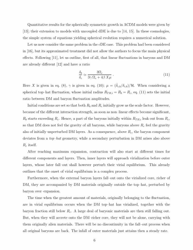
FIG. 6: Ratio between DM and baryon mass in virialized halos, against the value used for δc,rc

(DM masses are rescaled to the value they reach at τo. The dashed line is the background Ωc/Ωb

ratio.

In Figure 4 we plot the β dependence of δ(c)c,rc and δ(b)c,rc , at z = 0. They start from equal

values for β = 0 and gradually split as β increases. In Figure 5 we plot the z dependence of

δ(c)c,rc and δ(b)c,rc for β = 0.20 and 0.05. These values were computed by starting at z = 1000,

taking into account also the radiative component, and using the full set of equations.

Following the PS approach, the differential mass function then reads

ψ(M) = 2ρ

M

∫

∞

δc,rcdδM

dσMdM

d

dσM

1√2πσM

e−δ2M

/2σ2

M

=

√

2

π

ρ

M

∫

∞

δc,rc/σM

dνMdνMdM

νMe−ν2

M/2 . (26)

Here νM = δM/σM and δc,rc can be either δ(c)c,rc or δ(b)c,rc (or any intermediate value) according

to Fig. 4 and 5; a choice shall be based on the observable to be fitted.

The ST expression is obtainable from eq. (26) through the replacement

νM exp(−ν2M/2) → N ′ ν ′M(1 + ν ′−3/5M ) exp(−ν ′2M/2) , (27)

with N ′ = 0.322 , ν ′2M = 0.707 ν2M ,

14

meant to take into account the effects of non–sphericity in the halo growth.

In the absence of coupling and baryon–DM segregation, the mass M in the PS and ST

expressions (26)–(27) is the mass originally in the top–hat, which will then be comprised

within a virial radius Rv, such that M/(4π/3)ρR3v = ∆v.

In the presence of coupling and segregation the situation is more complex. However, in-

dipendently of the value taken for δc,cr, the resulting virialized system will be baryon depleted.

Different possible δc,cr’s will correspond to different depletions, but the final system shall

however contain a smaller fraction of baryons, in respect the background Ωb/Ωc ratio.

It is important to distinguish between two effects: (i) DM mass variation. (ii) The

dynamics of gravitational growth. Let Mi and Mvir be the masses, at the initial time and

at virialization, rescaled to the values they will have at τo, so that the (i) effect is isolated.

Then, while

Mi =M ci +M b

i = (Ωc/Ωm)Mi + (Ωb/Ωm)Mi , (28)

so that M ci /M

bi = Ωc/Ωb , in the decomposition

Mvir =M cvir +M b

vir (29)

it will however be M cvir/M

bvir > Ωc/Ωb .

Let us now duly take into account also the (i) effect and consider the case when the

mass function is set by δ(c)c,rc. Then, while M cvir/M

ci = exp[−C(φvir − φi)], it will obviously

be M bvir < M b

i : several baryon layers, initially belonging to the fluctuation, have not yet

recollapsed or virialized.

Let us then consider the mass function set by δ(b)c,rc. In this case it is M bvir = M b

i , but it

will be M cvir/M

ci > exp[−C(φvir − φi)]. The extra DM mass is due to those layers, initially

external to the fluctuation, first compressed and then conveyed inside the virialization radius,

together with the baryons previously outflown from the DM bulk.

For any δc,rc in the δ(c)c,rc–δ(b)c,rc interval, some baryon layers will still be out and some extra

DM will have been conveyed inside the virial radius by the fall out of outflown baryons.

Hence, it will however be M cvir exp[−C(φo − φvir] /M

bvir > Ωc/Ωb .

In Figure 6 we plot this ratio, as a function of δc,rc, in the δ(c)c,rc–δ(b)c,rc interval. The plot

shows that, after a fast decrease, the ratio tends to a steady value, however exceeding the

background ratio. The curves shown in this plot depend on the assumed (top–hat) shape

for the primeval fluctuation, but similar curves would hold for any initial shape.

15

A prediction of cDE theories, therefore, is that Ωc/Ωb, measured in any virialized struc-

ture, exceeds the background ratio. The excess is greater for structures where only DM has

virialized. They might be characterized by an apparent disorder in the baryon component,

still unsettled in virial equilibrium while, e.g., a lensing analysis would show that they are

safely bound systems.

We shall now plot mass functions obtained using either δ(c)c,rc or δ(b)c,rc. We expect ac-

tual measures to yield a value comprised in this interval and, however, closer to the δ(c)c,rc

curve when baryon stripping is stronger. In Figure 7 we plot the integral mass functions

n(>M) =∫

∞

M dM ′ ψ(M ′) obtained through ST expressions (26)–(27). Let us remind that

large differences between models were never found in mass functions at z = 0, because of

DE nature. The upper panel of each figure shows the mass function in the usual fashion,

as often plotted to fit data or simulations. In the lower panel we plot the ratio between

expected halo numbers for each model and ΛCDM. This confirms the small shifts between

ΛCDM and dDE cosmologies, yielding just a slight excess, ∼ 10%, on the very large cluster

scale, where observed clusters are a few units.

Discrepancies can be more relevant between ΛCDM and cDE, whose effective mass func-

tion should however lie inside the dashed areas, limited by the function obtained by inte-

grating from δ(c)c,rc or δ(b)c,rc . The plots show a shortage of larger clusters. For β = 0.20, they

are half of ΛCDM at ∼ 3 · 1014h−1M⊙ and really just a few above some 1015h−1M⊙ . Any

realistic mass function, laying in the dashed area, can be falsified by samples just slightly

richer than those now available.

For β = 0.05 the shift is smaller, hardly reaching 20%, still in the direction opposite to

dDE. Here we meet what appears to be a widespread feature of cDE models: the discrepancy

of dDE from ΛCDM is partially or totally erased even by a fairly small DM–DE coupling,

and many cDE predictions lay on the opposite side of ΛCDM, in respect to dDE. If a ΛCDM

model is then used to fit galaxy or cluster data arising in a cDE cosmology, we expect cluster

data to yield a best–fit σ8 value smaller than the one obtained by fitting galaxy data.

The integral mass functions obtained through the original PS expression are shown in

Fig. 8. This figure shows just slight quantitative shifts. In the cases illustrated by the next

figures, results from PS expression will be therefore omitted.

Figure 9 compares RP results with SUGRA, at z = 0. Quantitative differences exist,

when the self–interaction potential is changed, but most physical aspects are the same.

16

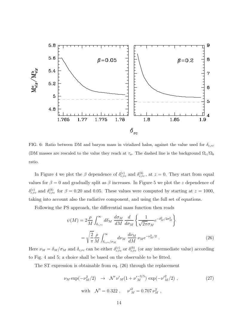
Sheth & Tormen

FIG. 7: Cluster per (Mpc h−1)3, above mass M at z = 0, obtained from ST expression. Four

models are considered, with equal Ω’s and h: ΛCDM, uncoupled SUGRA with Λ = 100MeV, and

two cDE with different β’s. The dashed areas are limited by the mass functions worked out for

δ(c)c,rc or δ

(b)c,rc in cDE models (see text).

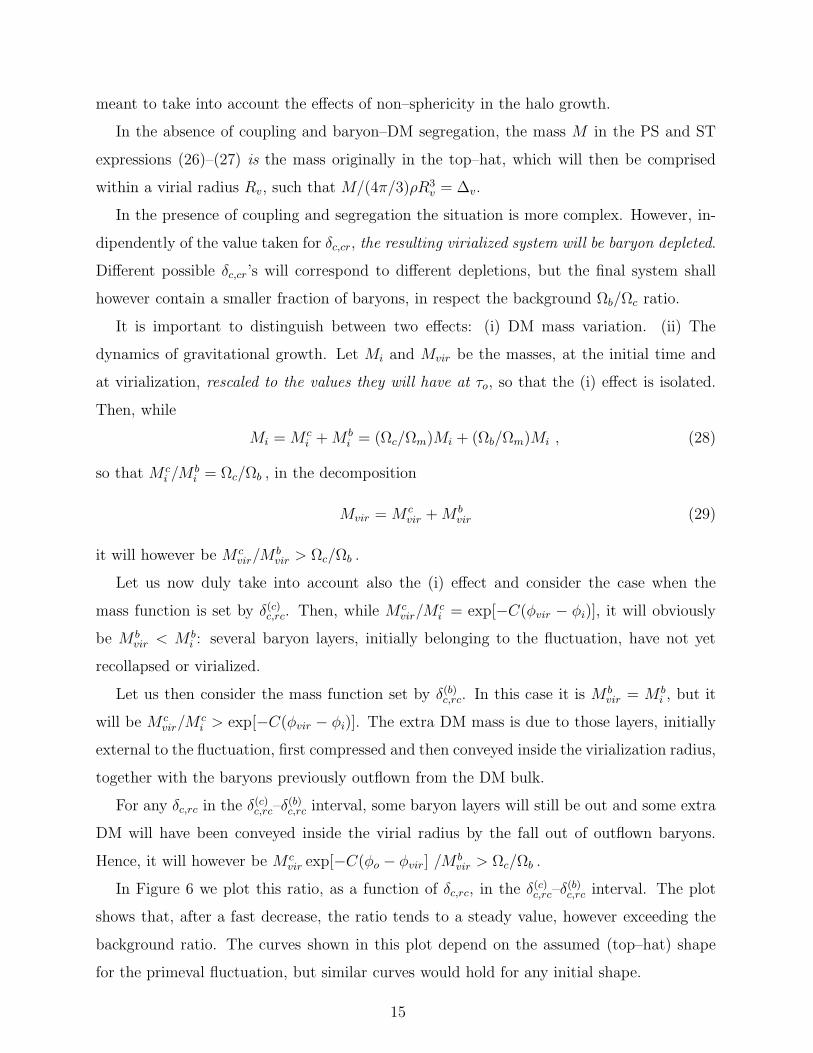
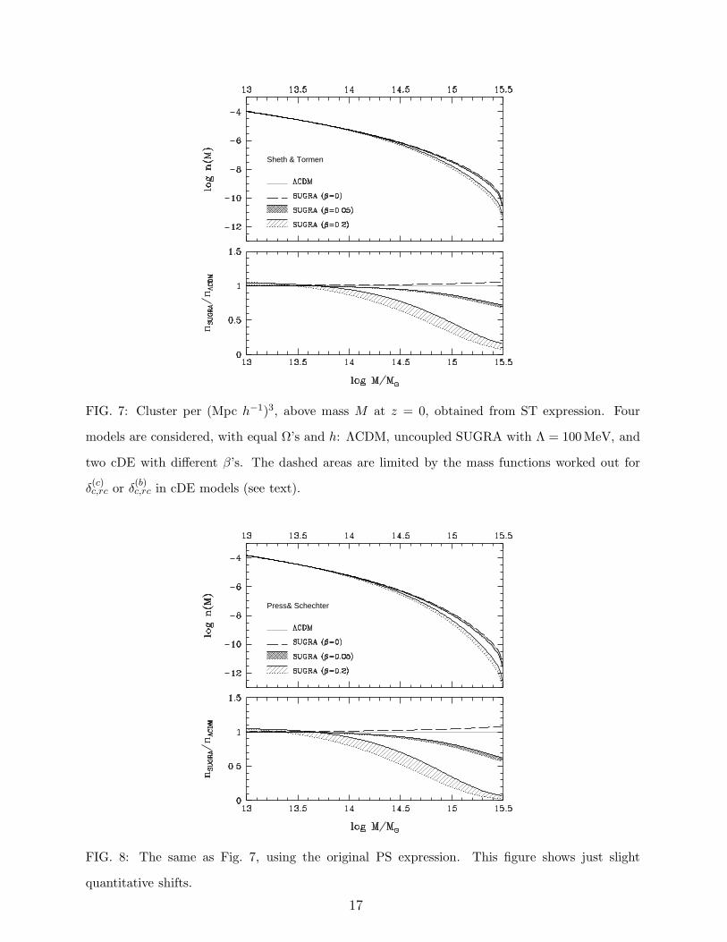
Press& Schechter

FIG. 8: The same as Fig. 7, using the original PS expression. This figure shows just slight

quantitative shifts.

17

FIG. 9: A comparison of SUGRA and RP results at z = 0 using the ST expression. The lower

panel of Fig. 7 is reproduced, neglecting dDE and β = 0.05 cases and adding RP results (heavy

dashed).

FIG. 10: Cluster per (Mpc h−1)3, above mass M at different z’s, in a fixed comoving volume,

obtained from ST expression. Thick solid and dotted lines refer to cDE models. The dashed

(thinner solid) line refers to dDE (ΛCDM).

18

FIG. 11: Evolution of the DM/baryon background ratio, due to the dynamics of the φ field.

In Figure 10 the redshift dependence of the expected cluster numbers in a comoving

volume is plotted against the redshift z, for M = 1014 and 4 · 1014h−1M⊙. As usual, the

mass considered is the total cluster mass. As already widely outlined, the DM/baryon ratio

in these masses however exceeds the background Ωb/Ωc ratio; the spread of the function

corresponds to the spread of possible baryon/DM ratios. In top of that, however, one

must also remind that the very background Ωc/Ωb ratio varies with redshift, because of the

evolution of the φ field. Hence, clusters observed at high z, in average, shall be however

baryon poorer than present time clusters. The z dependence of the background Ωc/Ωb ratio,

for the model considered in this work, is plotted in Figure 11.

Plots similar to Figure 10 are often used to assert the possibility to discriminate between

models and this plot is however significant to compare cDE with former results for other

cosmologies. According to [17], however, the discriminatory capacity of this observable can

only be tested by plotting cluster numbers per solid angle and redshift interval, which also

includes geometrical effects, often partially erasing dynamical effects.

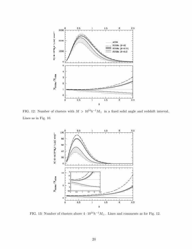
In the upper panels of Figures 12 and 13 cluster numbers per solid angle and redshift

interval are plotted. In the lower panels we plot the ratios between each SUGRA model and

ΛCDM mass functions. We consider again the mass scales 1014 and 4 · 1014h−1M⊙; for the

latter mass we provide a magnified box to follow the expected low–z behavior. Notice, in

particular, that the high–z behaviors for β = 0.05 or 0.2, for these mass scales, lay on the

opposite sides of ΛCDM. The box in Fig. 13 show how we pass from numbers smaller than

19

FIG. 12: Number of clusters with M > 1014h−1M⊙ in a fixed solid angle and redshift interval.

Lines as in Fig. 10.

FIG. 13: Number of clusters above 4 · 1014h−1M⊙ . Lines and comments as for Fig. 12.

20

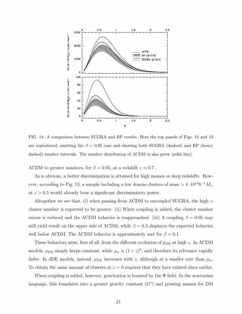
FIG. 14: A comparison between SUGRA and RP results. Here the top panels of Figs. 12 and 13

are reproduced, omitting the β = 0.05 case and showing both SUGRA (dashed) and RP (heavy

dashed) number intervals. The number distribution of ΛCDM is also given (solid line).

ΛCDM to greater numbers, for β = 0.05, at a redshift z ≃ 0.7 .

As is obvious, a better discrimination is attained for high masses or deep redshifts. How-

ever, according to Fig. 13, a sample including a few dozens clusters of mass > 4 ·1014h−1M⊙

at z > 0.5 would already bear a significant discriminatory power.

Altogether we see that, (i) when passing from ΛCDM to uncoupled SUGRA, the high–z

cluster number is expected to be greater. (ii) When coupling is added, the cluster number

excess is reduced and the ΛCDM behavior is reapproached. (iii) A coupling β = 0.05 may

still yield result on the upper side of ΛCDM, while β = 0.2 displaces the expected behavior

well below ΛCDM. The ΛCDM behavior is approsimately met for β = 0.1.

These behaviors arise, first of all, from the different evolution of ρDE at high z. In ΛCDM

models, ρDE simply keeps constant, while ρm ∝ (1 + z)3, and therefore its relevance rapidly

fades. In dDE models, instead, ρDE increases with z, although at a smaller rate than ρm.

To obtain the same amount of clusters at z = 0 requires that they have existed since earlier.

When coupling is added, however, gravitation is boosted by the Φ field. In the newtonian

language, this translates into a greater gravity constant (G∗) and growing masses for DM

21

particles. This speeds up cluster formation and, when β increases, less clusters are needed

at high z, to meet their present numbers.

Finally, in Figure 14 we provide a comparison between the PS–ST mass function obtain-

able for RP and SUGRA potentials. Only the case β = 0.2 is considered. A RP potential

slightly strengthens the effects already seen for SUGRA; as a matter of fact, however, in

most cases we find just small quantitative shifts.

CONCLUSIONS

In this work we aimed at predicting the cluster mass function in cDE cosmologies, by

using the solution of the equations ruling the spherical growth of top–hat fluctuations in ST

(or PS) expressions. The effectiveness of ST expressions has been widely verified for SCDM,

ΛCDM and 0CDM models. Also in simulations of models with dynamical (uncoupled) DE

[19], ST expressions provide a fair fit of numerical outputs.

The main finding of this study is the significant baryon–DM segregation, which has

multiple effects. If cluster numbers are measured from their gravitational effects, e.g., by

using lensing data, a PS–ST approach yields simple predictions. When cluster numbers are

measured through other observables, we predict a number range, inside which observations

should lie. The actual amount of objects, inside these ranges, is determined by a number of

effects, that a PS–ST approximation cannot describe.

An important example of such effects is the possible stripping of outer layers, in close

encounters, which will mostly act on the baryon component. For a rather small coupling as

β = 0.2, up to 40% of the baryons belonging to the initial fluctuation could be stripped in

this way and, even for the tiny coupling set by β = 0.05, 10% of baryons could be easily

stripped.

If cluster data are obtained from galaxy counts or hot gas features, they will exhibit the

residual baryon amount. Indipendently of the baryon loss, which depends on the individual

cluster history, cDE theories predict that the background Ωc/Ωb ratio however increases with

redshift. However, in top of that, the DM/baryon ratio measured in any virialized structure,

exceeds the background ratio at the redshift where it is observed and is expected to exhibit

significant variations in different systems, being smaller in larger systems, in average.

It must be however outlined that the final baryon/DM ratio, in any galaxy cluster at

22

any redshift, even in the absence of any stripping effect, is expected to by smaller than the

background Ωb/Ωc ratio at that redshift. In this paper dedicated to a technical analysis

of cDE mass functions we refrain from discussing this feature in further detail, although

relating it with the apparent baryon shortage in clusters, (see, e.g., [18]) seems suggestive.

Furthermore, when cluster data are obtained through the hot gas behavior, a complex

interplay between baryons and potential well is expected. Once again, however, the model

used for PS–ST estimates seems unsuitable to provide quantitative predictions, but anoma-

lies in the temperature–luminosity relations are expected.

A PS–ST analysis allows however to formulate further predictions, besides those con-

cerning the Ωb/Ωc ratio in galaxy clusters and in galaxies. They concern the cluster mass

function and its evolution.

No large differences between models were ever found in the mass functions at z = 0,

because of DE nature: just a slight excess, ∼ 10%, on the very large cluster scale, where

observed clusters are a few units, was found in dDE, in respect to a ΛCDM cosmology.

Discrepancies can be more relevant between ΛCDM and cDE, where a shortage of larger

clusters is predicted. For β = 0.20, they are half of ΛCDM at ∼ 3 ·1014h−1M⊙ and less than

20% above a few 1015h−1M⊙ . Such strong shortage can be falsified by samples just slightly

richer than those now available. For β = 0.05 the shift is smaller, hardly reaching 20%, but

still in the direction opposite to dDE.

This is a widespread feature of cDE models: the discrepancy of dDE from ΛCDM is

partially or totally erased even by a fairly small DM–DE coupling, and many cDE predictions

lay on the opposite side of ΛCDM, in respect to dDE. Therefore, if a ΛCDM model (or any

uncoupled model) is used to fit galaxy or cluster data arising in a cDE cosmology, we expect

that cluster data may yield a smaller σ8, in comparison to the one worked out from other

data sets.

Turning to the evolutionary predictions, we expect an evolution faster than ΛCDM for

any coupling β > 0.1, again the opposite of what we expect in uncoupled dDE.

Most quantitative results given in this paper are worked out by assuming that the scalar

field self–interaction potential is SUGRA, with Λ = 100GeV. For the sake of comparison,

in a few plots, results obtained for a RP potential are also shown. It should be reminded

that, while the former potential predicts a linear behavior consistent with observations, the

latter one can be fitted with linear observables only for quite low values of Λ, much below

23

the one considered here; we selected it just to provide a direct comparison tool, so allowing

us to conclude that a different self–interacion potential may cause quantitative shifts up to

some 10%, but hardly affect our general conclusions.

Altogether, there can be no doubt that cDE cosmologies open new prespectives for the

solution of those problems where baryon–DM segregation due to hydrodynamics is appar-

ently insufficient to explain observed features. These problems may range from the shortage

of galaxy satellites in the local group, to galactic disk formation, up to the L vs T relation

in large clusters. Stating how coupling can affect these and similar questions, by using a

PS–ST approach, is hard. This calls for detailed n–body and hydrodynamical simulations

of cDE cosmologies.

ACKNOWLEDGMENTS

Luca Amendola, Andrea Maccio and Loris Colombo are gratefully thanked for their

comments on this work.

[1] Wetterich C. 1988, Nucl.Phys.B 302, 668

[2] Ratra B. & Peebles P.J.E., 1988, Phys.Rev.D 37, 3406; Peebles P.J.E. & Ratra B., 1988, ApJ.

Lett., 325, L17

[3] Peebles P.J.E & Ratra B., 2003, Rev. Mod. Phys., 75, 559

[4] Amendola L., 1999, Phys. Rev. D60, 043501

[5] Amendola L. & Quercellini C., 2003, Phys. Rev. D68, 023514

[6] Maccio’ A. V., Quercellini C., Mainini R., Amendola L., Bonometto S. A., 2004 Phys. Rev.

D69, 123516

[7] Mainini R., Bonometto S.A., 2004, Phys.Rev.Lett. 93, 121301; Mainini R., Colombo L. &

Bonometto S.A., 2005, ApJ 635, 691-705

[8] Press W.H. & Schechter P., 1974, ApJ, 187, 425

[9] Sheth R.K. & Tormen G., 1999 MNRAS, 308, 119; Sheth R.K. & Tormen G., 2002 MNRAS

329, 61; Jenkins, A., Frenk C.S., White S.D.M., Colberg J.M., Cole S., Evrard A.E., Couchman

H.M.P. & Yoshida N., 2001, MNRAS, 321, 372

24

[10] Brax, P. & Martin, J., 1999, Phys.Lett., B468, 40; Brax, P. & Martin, J., 2000, Phys.Rev.

D61, 103502; Brax P., Martin J., Riazuelo A., 2000, Phys.Rev. D62, 103505

[11] Mainini R., 2005, PRD 72, 083514 (paper I)

[12] Amendola L., Phys. Rev. 2004, D69, 2004, 103524

[13] Lahav, O., Lilje, P.R., Primack, J.R. & Rees, M., 1991, MNRAS, 251,128; Brian, G. &

Norman, M., 1998, ApJ, 495, 80

[14] Mainini R., Maccio’ A. V., Bonometto S. A., 2003, New Astron., 8, 173 Mainini R., Maccio’

A. V., Bonometto S. A., Klypin A., 2003, ApJ, 599, 24

[15] Wang L. & Steinhardt P.J., 1998, ApJ, 508, 483; Lokas E. L., Bode P., Hoffman Y., 2004,

MNRAS, 349, 595 Horellou C., Berge J., 2005, astro-ph/0504465 Nunes N. J., da Silva A. C.,

Aghanim N., 2005, astro-ph/0506043

[16] Nunes N. J.& Mota D.F, 2005, astro-ph/0409481 Manera M. & Mota D., 2005,

astro-ph/0504519

[17] Solevi P., Mainini R., Bonometto S.A., Maccio’ A.V., Klypin A., Gottloeber S., 2006 MNRAS

366, 1346

[18] Allen S.W., Schmidt R.W., Fabian A.C., 2001, MNRAS 328, l37, Ettori S., 2003, MNRAS

344, L13

[19] Klypin A., Maccio A., Mainini R. & Bonometto S.A., 2003 ApJ 599, 31

25

Appendix 1. The newtonian regime

In the presence of inhomogeneities, the metric can read

ds2 = a2(τ)[−(1 + 2ψ)dτ 2 + (1− 2ψ)dxidxi], (30)

provided that no anisotropic stresses are considered, ψ being the gravitational potential in

the Newtonian gauge. Let us describe DE field fluctuations δφ through

ϕ = (4π/3)1/2 (δφ/mp) (31)

and expand fluctuations in components of wavenumber k; let also be λ = H/k. Let then be

f = φ−1√

3/16πG ln(V/Vo), f1 = φdf

dφ+ f, f2 = φ

df

dφ+ 2f + f1 ; (32)

Vo being a reference value of the potential. It is also useful to define Y 2 = 8πGV (φ) a2/3H2.

The equations ruling the evolution of the ϕ field and gravity, keeping just the lowest order

terms in λ, as is needed to obtain their Newtonian limit, then read

ψ = −3

2λ2(Ωbδb + Ωcδc + 6Xϕ+ 2Xϕ′ − 2Y 2f1 ϕ) , ψ′ = 3xϕ− ψ , (33)

ϕ′′ + (2 +H′

H )ϕ′ + λ−2ϕ− 12Xϕ+ 4ψX + 2Y 2(f2ϕ− f1ψ) = βΩc(δc + 2ψ) ; (34)

let us remind that X is defined in eq. (8) and notice that, if DE kinetic (and/or potential)

energy substantially contributes to the expansion source, X (and/or Y ) is O(1).

In the Newtonian limit, ϕ derivatives shall be neglected, the oscillations of ϕ and the

potential term f2Y2ϕ should be averaged out, by requiring that λ << (f2Y )−1, and, in

eq. (34), the metric potential ψ (∝ λ2) can also be neglected. Then, eqs. (33)–(34) become

ψ = −3

2λ2(Ωbδb + Ωcδc), , λ−2ϕ ≃ βΩcδc. . (35)

Baryon and DM density fluctuations are then ruled by the eqs. (6)–(7), derived from the

stress–energy pseudo–conservation T µν;µ = 0. Thereinside, ′ yields differentiation with respect

to ln a. [Let us then notice that, taking Ωb << Ωc, putting δc ∝ e∫

µ(α)dα and δb = bδc with

b = cost , eqs. (6), allow us to obtain the bias factor (11)].

The acceleration of a DM or baryon particle of mass mc,b can then be derived from

eqs. (6)–(7). Let it be in the void, at a distance r from the origin, where a DM (or baryon)

particle of mass Mc (or Mb) is set, and let us remind that, while ρb ∝ a−3, it is

ρc = ρoca−3e−C(φ−φ0), ρMc

=Moca−3e−C(φ−φ0)δ(0), (36)

26

because of the DE–DM coupling (the subscript o indicates values at the present time τo;

let also be ao = 1). We can then assign to each DM particle a varying mass Mc(φ) =

Moce−C(φ−φ0)

Then, owing to eq. (36), and assuming that the density of the particle widely exceeds the

background density, it is

Ωcδc =ρMc

− ρcρcr

=8πG

3H2aMc(φ)δ(0) , Ωbδb =

ρMb− ρbρcr

=8πG

3H2aMbδ(0), (37)

(ρcr is the critical density and δ is the Dirac distribution). Reminding that ∇ · vc,b = θc,bHand using the ordinary (not conformal) time, eq. (6) yields

∇ · vc = −H(1− 2βX)∇ · vc − 4πGa−2 (γMc(φ) +Mb) δ(0) (38)

(dots yield differentiation in respect to ordinary time and H = a/a). Taking into account

that the acceleration is radial, as the attracting particles are in the origin, it will be

∫

d3r∇ · v = 4π∫

dr d(r2v)/dr = 4πr2v.

Accordingly, the radial acceleration of a DM particle is

vc = −(1− 2βX)Hvc · n− G∗Mc(φ)

R2− GMb

R2, (39)

(n is a unit vector in the radial direction; R = ar).

By following a similar procedure for baryons, we obtain:

vb = −Hvb · n− GMc(φ)

R2− GMb

R2(40)

In the presence of full spherical symmetry, vb,c · n = vb,c; being then b = rb and c = rc,

eqs. (14) immediately follow.

For the sake of completeness, here below, we write also the equations for the physical

DM and baryons radii which easily follow from eqs. (39) and (40). While for baryons we

have the usual Friedman-like equations

Rnb = −4π

3G [ρc + ρb + ρDE(1 + 3w)] Rn

b , (41)

for DM we have

Rnc = CφRn

c − CφHRnc −

4π

3G [ρc + γ(ρc − ρc) + ρb + ρDE(1 + 3w)] Rn

c . (42)

27