University of Ljubljana Faculty of Mathematics and Physics Department of Meteorology Seminar: 4th class Turbulence kinetic energy - TKE Author: Matic Šavli Mentor: doc. dr. Nedjeljka Žagar May 27, 2012 Abstract In this seminar I present the measure of turbulence in the atmosphere. This is the so called turbulent kinetic energy (TKE). Most of our life is spent in the lower layers of atmosphere. The lovest layer of the atmosphere is called boundary layer (BL). In average this layer occupies from 100 m to few kilometers of atmosphere. First I present some basic concepts of boundary layer. Then I introduce the concept of spectral-gap and Reynolds averaging that represent the starting point of theoretical treatment of turbulence. There is following the theoretical derivation of TKE budget equation and explanation of the most important mechanisms for the production of turbulence. At the end, I present a slightly different perspective on the turbulent kinetic energy. This reveals some interesting properties of turbulence in the boundary layer.
Transcript
University of LjubljanaFaculty of Mathematics and Physics
Department of Meteorology
Seminar: 4th class
Turbulence kinetic energy - TKE
Author: Matic ŠavliMentor: doc. dr. Nedjeljka Žagar
May 27, 2012
Abstract
In this seminar I present the measure of turbulence in the atmosphere. This is the so calledturbulent kinetic energy (TKE). Most of our life is spent in the lower layers of atmosphere. Thelovest layer of the atmosphere is called boundary layer (BL). In average this layer occupies from 100m to few kilometers of atmosphere. First I present some basic concepts of boundary layer. Then Iintroduce the concept of spectral-gap and Reynolds averaging that represent the starting point oftheoretical treatment of turbulence. There is following the theoretical derivation of TKE budgetequation and explanation of the most important mechanisms for the production of turbulence. Atthe end, I present a slightly different perspective on the turbulent kinetic energy. This reveals someinteresting properties of turbulence in the boundary layer.
Turbulence is a type of fluid (gas or liquid) flow in which the fluid undergoes irregular fluctuations, ormixing, in contrast to laminar flow, in which the fluid moves in smooth paths or layers. In turbulentflow the speed of the fluid at a point is continuously undergoing changes in both magnitude anddirection [1]. Turbulence can be visualized as consisting of irregular swirls of motions called eddies.Usually turbulence consists of many different size eddies superimposed on each other. The relativestrengths of these different scale eddies define the turbulent spectrum (see next chapter). Figure 1presents some examples of visual representations of turbulence.
Figure 1: Visual representation of turbulent eddies. Laminar flow of cigarette smoke becoming turbulent, on the left picture. Flowvisualization of a turbulent jet, made by laser-induced fluorescence, on the right picture [2, 3].
Turbulence in the atmosphere is very important feature especially for aviation. Figure 2 shows in-tensity of the so-called CAT (Clear Air Turbulence) at height in range 3 to 15 km. Clear-air turbulenceis a higher altitude (6 - 15 km) turbulence phenomenon occurring in cloud-free regions, associated withwind shear, particularly between the core of a jet stream and the surrounding air [4].
1
Figure 2: The maximum amount of turbulence (CAT) one can expect in any given area of the US, from altitudes 20,000 (6 km)feet to 45,000 feet (12 km). A typical flight cruises at around 35,000 feet (10 km). [5].
The intensity of turbulence presented in the above figures is actually directly related to the so-called turbulent kinetic energy (TKE). As is apparent from the name of this quantity, the value ofTKE directly represents the ’strength’ of the turbulence in the flow. Turbulence and turbulent kineticenergy are strongly related to the wind shear (see in the following chapters), especially in the case ofCAT. This means that in the case of clear air turbulence intensity of turbulence is strongly dependenton the value of the horizontal velocity field shear. Obviously TKE is a very important quantity.
In the following sections I will describe the main features of turbulent kinetic energy. More im-portantly, I will deal with TKE budget equation and its terms. These terms in more detail explainthe mechanisms that directly affect the intensity of the turbulence. Figure 2 shows the example ofClear-Air-Turbulence, but in this seminar the turbulence in lower layers of the atmosphere will bepresented. This is the so-called boundary layer. Let us firstyl look at some of the characteristics ofthis layer.
2 Boundary layer
Boundary layer (PBL, BL) is that part of the atmosphere that is directly influenced by the presenceof the earth’s surface, and responds to surface forcings with a timescale of about an hour or less [6].This will be further explained in the next chapter.
Symbolic view of the atmosphere structure is shown on the left picture in Fig. 3. An example oftemperature variations in the lower troposphere is shown in the right picture in Fig. 3.
Figure 3: The troposphere can be divided into two parts: a boundary layer (blue) near the surface and the free atmosphere aboveit. Evolution of temperatures (picture on the right) measured near the ground (975 mbar) and at the a height of roughly 1100 mabove ground. [7] [6].
2
Time-history in Fig. 3 were constructed from sond-soundings made every several hours near Law-ton, Oklahoma. They show a diurnal-variation of temperature at two different heights above ground.Diurnal variations at greater altitudes are much less intense because the turbulence is less intense.Such variation is one of the key characteristics of the bundary layer.
Some of the most important features of PBL:
→ Significant drag against earth’s surface. High energy dissipation (due to friction).
→ Continuous turbulence throughout layer.
→ Thickness between 100 and 3000 m, diurnal variation over land.
→ Rapid turbulent mixing in vertical and horizontal.
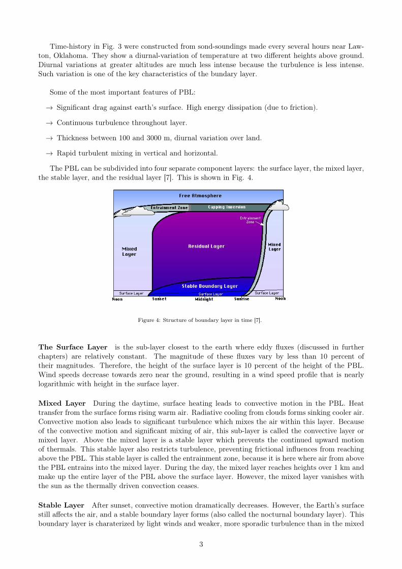
The PBL can be subdivided into four separate component layers: the surface layer, the mixed layer,the stable layer, and the residual layer [7]. This is shown in Fig. 4.
Figure 4: Structure of boundary layer in time [7].
The Surface Layer is the sub-layer closest to the earth where eddy fluxes (discussed in furtherchapters) are relatively constant. The magnitude of these fluxes vary by less than 10 percent oftheir magnitudes. Therefore, the height of the surface layer is 10 percent of the height of the PBL.Wind speeds decrease towards zero near the ground, resulting in a wind speed profile that is nearlylogarithmic with height in the surface layer.
Mixed Layer During the daytime, surface heating leads to convective motion in the PBL. Heattransfer from the surface forms rising warm air. Radiative cooling from clouds forms sinking cooler air.Convective motion also leads to significant turbulence which mixes the air within this layer. Becauseof the convective motion and significant mixing of air, this sub-layer is called the convective layer ormixed layer. Above the mixed layer is a stable layer which prevents the continued upward motionof thermals. This stable layer also restricts turbulence, preventing frictional influences from reachingabove the PBL. This stable layer is called the entrainment zone, because it is here where air from abovethe PBL entrains into the mixed layer. During the day, the mixed layer reaches heights over 1 km andmake up the entire layer of the PBL above the surface layer. However, the mixed layer vanishes withthe sun as the thermally driven convection ceases.
Stable Layer After sunset, convective motion dramatically decreases. However, the Earth’s surfacestill affects the air, and a stable boundary layer forms (also called the nocturnal boundary layer). Thisboundary layer is charaterized by light winds and weaker, more sporadic turbulence than in the mixed
3
layer. The height of the PBL, therefore, decreases significantly during the night. Though the height ofthe nocturnal layer varies, it is usually less than half that of the mixed layer. Unlike the mixed layer,the stable boundary layer does not have a well-defined top. Instead, it slowly merges with the residuallayer.
Residual Layer As turbulence and the mixed layer decay with sunset, the air maintains many ofthe state variables that the well-mixed air had. This layer is called the residual layer (because itsproperties are residuals of the mixed layer) and forms above the stable boundary layer. While thenocturnal boundary layer has a very stable profile, the residual layer tends to have more of a neutralprofile. The residual layer does not have contact with the earth’s surface, and so is not influencedby turbulent stresses like the stable boundary layer below it. The residual layer is bounded above bya capping inversion, which approximates the height of the daytime height of the mixed layer. Thisinversion simply prevents entrainment from aloft.
3 Turbulence spectrum and spectral gap
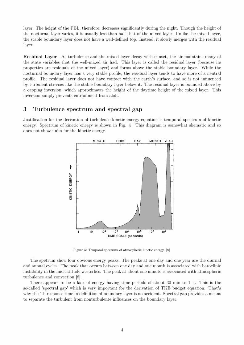
Justification for the derivation of turbulence kinetic energy equation is temporal spectrum of kineticenergy. Spectrum of kinetic energy is shown in Fig. 5. This diagram is somewhat shematic and sodoes not show units for the kinetic energy.
Figure 5: Temporal spectrum of atmospheric kinetic energy. [8]
The spetrum show four obvious energy peaks. The peaks at one day and one year are the diurnaland annual cycles. The peak that occurs between one day and one month is associated with baroclinicinstability in the mid-latitude westerlies. The peak at about one minute is associated with atmosphericturbulence and convection [8].
There appears to be a lack of energy having time periods of about 30 min to 1 h. This is theso-called ’spectral gap’ which is very important for the derivation of TKE budget equation. That’swhy the 1 h response time in definition of boundary layer is no accident. Spectral gap provides a meansto separate the turbulent from nonturbulente influences on the boundary layer.
4
4 Mean and turbulent part
The method of separation turbulent from nonturbulent flow is signal averaging over period of 30 minto 1 h. That’s how we can separate turbulent scale motions from nonturbulent scale motions. Andthis is only possible because of existance of spectral gap. Nonturbulent part of the flow is presentedby equation:
A(s) =1
T
∫ T
0A(t, s)dt, (1)
where T is some value in the time interval of spectral gap, so 30 min to 1 h. Here s is some otherspatial variable and A is variable like temperature or velocity field.
This is the way to eliminate turbulent fluctuations of scales shorter than about 1 h from the signal.Once we have the mean (nonturbulent) part of the signal (A) we can substract it from the actual signal(A), to give us turbulent part of the signal (a′):
a′ = A−A (2)
Here a′ is not necessarily small, because equations (2,1) just represent the method of separation tur-bulent part from nonturbulent part of energy spectrum. But we can think of a′ as the fluctuation thatis superimposed on the mean (nonturbulent part).
From these equations it’s obvious that this kind of averaging is not so good for motions of scalesof about 1 h. This represents problems for larger scales of turbulence. But because of existance ofspectral gap this is not a problem, because there is no motions at those scales. That’s way spectralgap is so important.
Let A and B be two variables that are dependent on time, and let c represent a constant. Then wecan present some basic rules of averaging. This can be done by using equation 1. To summarize:
c = c
cA = cA
A = A
AB = AB
A+B = A+B (3)
4.1 Reynolds averaging
The averaging rules in equation 3 can now be applied to variables that are split into mean and turbulentparts. Let A = A+ a′ and B = B + b′ like in equation 2. Using third and fifth rule in equation 3 wecan see that:
A = (A+ a′) = A+ a′ = A+ a′
So the only way that the left and right sides can be equal is if a′ = 0. This result is not surprising ifone remembers the definition of mean value (equation 1). Similar to Ab′ = Ba′ = 0.
The most important feature of Reynolds averaging is presented with the following equation:
AB = (A+ a′)(B + b′)
= (A)(B) +Ba′ +Ab′ + a′b′
= (A)(B) + a′b′ (4)
Where previously defined equations were used. The nonlinear product a′b′ is not necessarily equal tozero. The same is true for other nonlinear variables such as: a′2, b′2, a′2b′ etc. Such variable is called
5
eddy or turbulent flux and is of primary importance for understanding turbulence. More about thatfollows below.
What is the reason that product like a′b′ is not necessarily equal to zero? One statistical measureof the dispersion of data is the variance σ2 defined by:
σ2A =
1
N
i=N−1∑i=0
(Ai −A)2 = a′2
Another statistical measure is covariance defined by:
covar(A,B) =1
N
i=N−1∑i=0
(Ai −A)(Bi −B) = a′b′
Thus, the nonlinear turbulence products that were introduced in equation 4 have the same meaningas dispersion or covariance. These two measures could be zero but this is true only for a few selectedcases. Similarly we can define correlation as rAB = a′b′/σAσB.
4.2 Additional features of Reynolds averaging
Reynolds averaging has one very important feature. Let say Ui = Ui + U ′i is velocity field (i∈[x, y, z])and A = A+ a′ is some variable, then:
dA
dt=∂A
∂t+ Ui
∂A
∂xi
=∂(A+ a′)
∂t+ (Ui + U ′i)
∂(A+ a′)
∂xi
dA
dt=∂A
∂t+ Ui
∂A
∂xi+ U ′i
∂a′
∂xi
Where Einstein’s notation of summation is used. In the last equation we can see additional term. Thisis advection of a′ with u′i. Now we use continuity equation where we assume incompressibility:
∂Ui∂xi
= 0 =⇒ ∂Ui∂xi
= 0∂U ′i∂xi
= 0 (5)
Where we already use rules from Reynolds averaging. Now let’s multiply last equation from system 5with a′. Then add this to dA/dt and we get:
dA
dt=∂A
∂t+ Ui
∂A
∂xi+∂a′u′i∂xi
(6)
So, total derivative consists of two parts. The first one is just total derivative of A, where advectionis driven by Ui. The second term is advection of a′ driven by U ′i or like in last equation it can alsobe described as the divergence of turbulent momentum flux (see next section). This means that whenwe want to calculate the average part of total derivative of A we also need to know something aboutturbulence. This means that the mean flow is directly influenced by turbulence. This is very similarconclusion as in equation 4.
5 Eddy flux
Fluid motion can transport quantities, resulting in fluxes. Turbulence also involves motion. Thus weexpect that turbulence transports quatities, too. This mechanisem is presented by terms similar toa′b′.
Let’s see an example where eddy flux is defined by w′Θ′. This is so-called turbulent heat flux.Where w′ is turbulent part of vertical velocity and Θ′ is turbulent part of potential temerature. The
6
potential temperature of a parcel of fluid at pressure p is the temperature that the parcel would acquireif adiabatically brought to a standard reference pressure p0, usually 1000 millibars. The potentialtemperature is defined by:
θ = T (p0
p)R/cp , (7)
where T is the current absolute temperature (in K) of the parcel, R is the gas constant of air, and cpis the specific heat capacity at a constant pressure. θ is simply the temperature that a parcel of dryair at pressure p and temperature T would have if it were expanded or compressed adiabatically to astandard pressure p0 [9].
A line of constant Θ presents where dry air particle can move.If turbulence is completely random, then a positive w′Θ′ one instant might cancel a negative w′Θ′
at some later instant, resulting in a near zero value for average turbulent heat flux. But there aresituations where the average turbulent heat flux might be significantly different from zero. This isshown in Fig. 6.
Figure 6: Small eddy mixing process. Net upward turbulent heat flux in a statically unstable (dΘ/dz < 0) environment (a) and(b) net downward turbulent heat flux in a stable (dΘ/dz > 0) environment. Gray arrows represents the upward/downward heattransfer. [6].
On a hot summer day (Fig. 6a) the average potential temperature profile is superadiabatic. Thismeans that atmosphere is statically unstable. So if some air particle is moved away from the equilibriumthere is now return or equivalent dΘ/dz < 0. If the eddy is a swirling motion, then some of the airfrom position 1 will be mixed downward (w′ < 0), while some air from position 2 will mix up (w′ > 0).The average motion caused by turbulence is w′ = 0. The downward moving air parcel (w′ < 0) ends upbeing cooler then its surroundings (Θ′ < 0, assuming that particle Θ was conserved during its travel),resulting in w′Θ′ > 0. The upward moving air (w′ > 0) is warmer then its surroundings (Θ′ > 0), alsoresulting in w′Θ′ > 0. Both the upward and downward moving air contribute positively to the fluxw′Θ′, thus the average kinematic eddy flux w′Θ′ is positive for this small-eddy mixing process.
This result shows that turbulence can cause a net transport of heat, even there is no net transportof mass (w′ = 0). Turbulent eddies transport heat upward in this case tending to make dΘ/dz moreadiabatic (dΘ/dz > 0).
Let’s see what happens on a night (Fig. 6b) where a statically stable lapse rate is present (dΘ/dz >0). There is small eddy moving air up (w′ > 0) and some back down (w′ < 0). An upward movingparcel ends up cooler then its surrounding (w′Θ′ < 0) while a downward moving parcel is warmer(w′Θ′ < 0). The net effect of this small-eddy mixing is to cause w′Θ′ < 0, meaning a downwardtransport of heat [6].
From both cases we can see that turbulence tends to destroy itself.
7
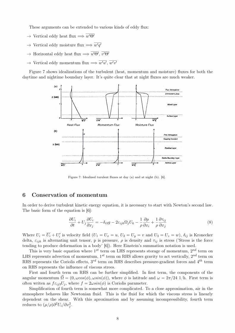
These arguments can be extended to various kinds of eddy flux:
→ Vertical eddy heat flux =⇒ w′Θ′
→ Vertical eddy moisture flux =⇒ w′q′
→ Horizontal eddy heat flux =⇒ u′Θ′, v′Θ′
→ Vertical eddy momentum flux =⇒ w′u′, w′v′
Figure 7 shows idealizations of the turbulent (heat, momentum and moisture) fluxes for both thedaytime and nightime boundary layer. It’s quite clear that at night fluxes are much weaker.
Figure 7: Idealized turulent fluxes at day (a) and at night (b). [6].
6 Conservation of momentum
In order to derive turbulent kinetic energy equation, it is necessary to start with Newton’s second law.The basic form of the equation is [6]:
∂Ui∂t
+ Uj∂Ui∂xj
= −δi3g − 2εijkΩjUk −1
ρ
∂p
∂xi+
1
ρ
∂τij∂xj
(8)
Where Ui = Ui + U ′i is velocity field (U1 = Ux = u, U2 = Uy = v and U3 = Uz = w), δij is Kroneckerdelta, εijk is alternating unit tensor, p is pressure, ρ is density and τij is stress (’Stress is the forcetending to produce deformation in a body’ [6]). Here Einstein’s summation notation is used.
This is very basic equation where 1st term on LHS represents storage of momentum, 2nd term onLHS represents advection of momentum, 1st term on RHS allows gravity to act vertically, 2nd term onRHS represents the Coriolis effects, 3rd term on RHS describes pressure-gradient forces and 4th termon RHS represents the influence of viscous strees.
First and fourth term on RHS can be further simplified. In first term, the components of theangular momentum ~Ω = (0, ωcos(φ), ωsin(φ)), where φ is latitude and ω = 2π/24 1/h. First term isoften writen as fεij3Uj , where f = 2ωsin(φ) is Coriolis parameter.
Simplification of fourth term is somewhat more complicated. To a close approximation, air in theatmosphere behaves like Newtonian fluid. This is the fluid for which the viscous stress is linearlydependent on the shear. With this aproximation and by assuming incompressibility, fourth termreduces to (µ/ρ)∂2Ui/∂x
2j .
8
7 Definition of TKE
Idea of turbulence kinetic energy is very similar to the idea of kinetic energy. Let’s say ~U is velocityfield. Then we can define ~U = ~U + ~U ′ like in equation 2. We can define two kinds of kinetic energy:
MKE/m =1
2(u2 + v2 + w2) (9)
TKE/m = e =1
2(u′2 + v′2 + w′2) =
1
2U ′2i (10)
The first equation represents kinetic energy of the mean flow (MKE) and second equation representskinetic energey of turbulent part of the flow (TKE). The second equation is also-called turbulent kineticenergy.
Turbulent kinetic energy is one of the most important variables in micrometeorology. It’s a measureof the intensity of turbulence. But since the turbulence may change in time we are more interested inTKE budget equation (∂e/∂t).
This equation is obtained from equation 8, in addition with equations 6 and 5. This gives us theTKE budget equation [6]:
∂e
∂t+ U j
∂e
∂xj= δi3
g
ΘU ′iΘ
′ − U ′iU ′j∂U i∂xj−∂U ′je
∂xj− 1
ρ
∂U ′ip′
∂xi− ε
This equation can be further simplified if we assume horizontal homogenity. So final version is:
∂e
∂t=g
Θw′Θ′ − U ′iw′
∂Ui∂z− ∂w′e
∂z− 1
ρ
∂w′p′
∂z− ε (11)
Turbulence is disspative, that’s why we have additional term ε. This term exists whenever TKE isnonzero. This means that turbulence will always tend to decrease and disappear with time. The otherterms are also very important. They represents physical processes that can increase/decrease TKEbudget in time.
7.1 Contribution to the TKE budget
Now let’s look at what all these terms in equation 11 represent.
Storage of TKE Figure 8 shows a simulation of TKE over a two day period. We can see a dramaticincrease/decrease of TKE within each diurnal cycle. Height is normalized with depth of mixed layer.
Figure 8: Modeled space/time variations of e. [6].
Variations of this term is also presented by figure 13 (bottom-right). We can see that TKE variesby about two orders of magnitude, mostly somewhere between night and day.
9
Figure 9: Normalized terms in the TKE budget equation. The shaded areas presents variation of particular terms at day. Heightvariable is normalized with depth of mixed layer (left figure). Right two pictures show TKE terms in cloud situation. [6].
Bouyancy term This term has two functions:
1. ProductionThe most important is temperature flux w′Θ′. This flux must be positive in the case of productionof TKE. As we have already seen, this is possible only in statically unstable atmosphere. Nearthe ground term 2 of equation 11 may be very large, corresponding to a large generation rateof turbulence whenever surface is warmer than the air. For sunny days over land or cold airadvection over warmer surface this term can be large in contrast to cloudy days. Simbolicallythis term is presented in Fig. 9. This figure clearly shows that term 2 is most important at theground where the temperature difference (air/ground) is the greater.
2. ConsumptionIn statically stable conditions, an air parcel displaced verticall by turbulence would experiencea bouyancy force pushing it back towards starting point. Statically conditions therby tends toconsume TKE, and are associated with negative values of temperature flux w′Θ′. Such conditionsare present in the stable boudary layer at night. There are some special cases where a region ofstatically stable layer could be somewhere in the cloud layer. This is presented on right picturein Fig. 9.
Because this term is so important on days of free convection, it is often used to normalize all theother terms in TKE equation, like the left picture in Fig. 9.
Mechanical Shear This term has two parts. First presents momentum flux and second presentsvertical shear of horizontal ’mean’ velocity. But important is interaction between this two parts. Eventhough a negative sign preceds 2nd term on RHS of equation 11 , the momentum flux is usually ofopposite sign from the mean shear, resulting in production of turbulence. So in the contrast to 1st term(RHS), this term is more like production term. In Fig. 9 we can see very large values of this term atthe surface (surface layer). The reason for this is in maximum shear at the surface. Wind speed varieslittle with height in the mixed layer of boundary layer above the surface layer, thats why small valuesof 2nd term (RHS) above surface layer. A smaller maximum of shear production sometimes occurs atthe top of the mixed layer, because of the increase of shear in entrainment zone.
Very important is relative contribution of the bouyancy term (1st term RHS) and shear term (2nd
term RHS) to the TKE budget. This can be used to classify the nature of convection (see figure 10).There are two options:
1. Free convection =⇒ |bouyancy| > |shear| and
2. Forced convection =⇒ |bouyancy| < |shear|.
10
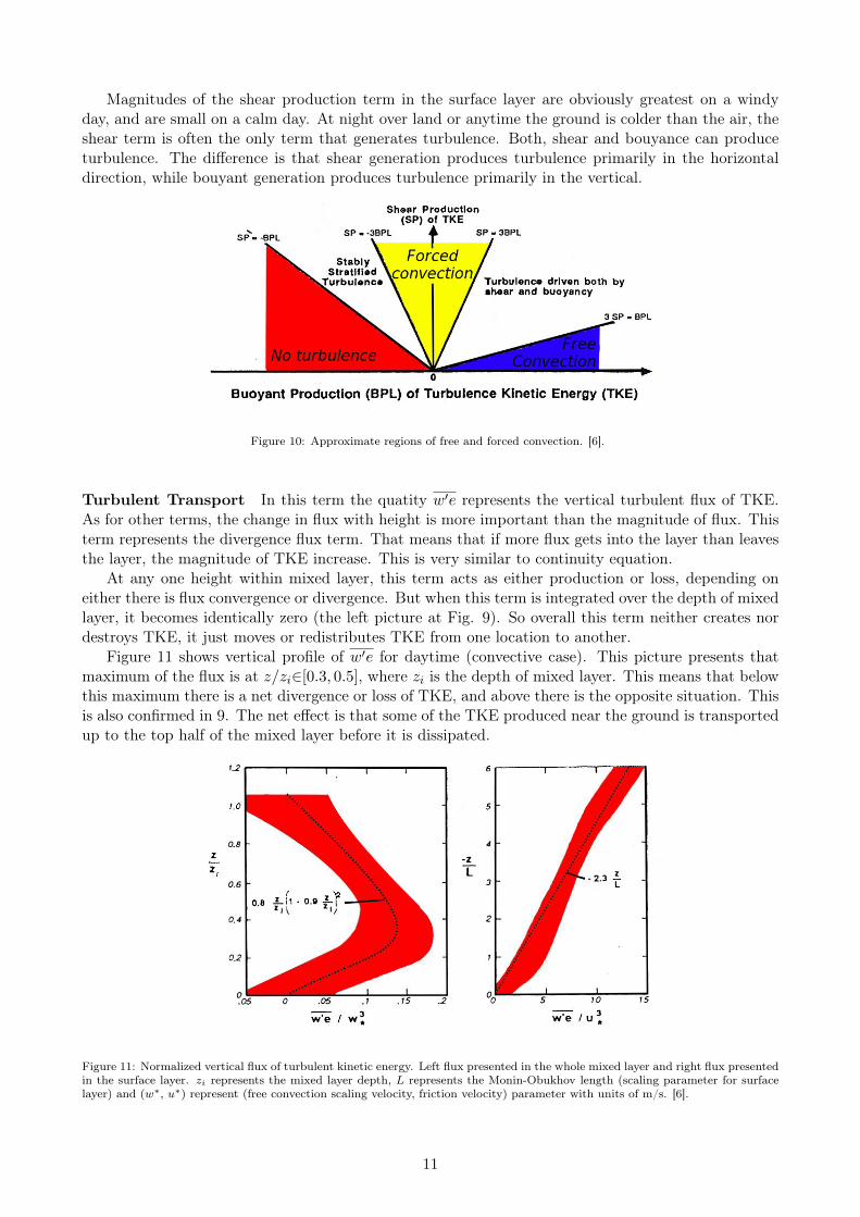
Magnitudes of the shear production term in the surface layer are obviously greatest on a windyday, and are small on a calm day. At night over land or anytime the ground is colder than the air, theshear term is often the only term that generates turbulence. Both, shear and bouyance can produceturbulence. The difference is that shear generation produces turbulence primarily in the horizontaldirection, while bouyant generation produces turbulence primarily in the vertical.
Figure 10: Approximate regions of free and forced convection. [6].
Turbulent Transport In this term the quatity w′e represents the vertical turbulent flux of TKE.As for other terms, the change in flux with height is more important than the magnitude of flux. Thisterm represents the divergence flux term. That means that if more flux gets into the layer than leavesthe layer, the magnitude of TKE increase. This is very similar to continuity equation.
At any one height within mixed layer, this term acts as either production or loss, depending oneither there is flux convergence or divergence. But when this term is integrated over the depth of mixedlayer, it becomes identically zero (the left picture at Fig. 9). So overall this term neither creates nordestroys TKE, it just moves or redistributes TKE from one location to another.
Figure 11 shows vertical profile of w′e for daytime (convective case). This picture presents thatmaximum of the flux is at z/zi∈[0.3, 0.5], where zi is the depth of mixed layer. This means that belowthis maximum there is a net divergence or loss of TKE, and above there is the opposite situation. Thisis also confirmed in 9. The net effect is that some of the TKE produced near the ground is transportedup to the top half of the mixed layer before it is dissipated.
Figure 11: Normalized vertical flux of turbulent kinetic energy. Left flux presented in the whole mixed layer and right flux presentedin the surface layer. zi represents the mixed layer depth, L represents the Monin-Obukhov length (scaling parameter for surfacelayer) and (w∗, u∗) represent (free convection scaling velocity, friction velocity) parameter with units of m/s. [6].
11
Figure 12: Normalized Doppler-radar derived deviation of perturbation pressure. [6].
Pressure Corelation Static pressure fluctuations are difficult to measure in the atmosphere. Themagnitudes of these fluctuations are very small, being on the order of 0.05 mb in the convectivesurface layer to 0.01 mb or less in mixed layer. For comparing, the standard pressure on sea level isp0 = 1013.25 mb. As a result, correlations (flux) such as w′p′ calculated from experimetal data oftencontain more noise than signal. We can estimate this flux from TKE equation but the result is notvery representative (huge variations). This is also confirmed by the Fig. 12. This figure shows thatpressure variation rapidly increase with height and at the top of mixed layer are realy quite large.
Figure 13: Top two pictures represent range of normalized dissipation rate (ε) during the day and night. Bottom left picturerepresents variation of dissipation rate with time. Bottom right picture represents variation of TKE in the surface layer with time.h represents depth of boundary layer. [6].
Dissipation This term presents the last term in equation 8. This term presents the so-called viscousdissipation and it is defined as:
ε = µ(∂w′
∂z)2 (12)
Where we considered only the vertical component and µ presents kinematic viscosity. It is obviousthat this term is always positive therefore this term always causing a decrease in the TKE budget.
12
In addition, it becomes larger in magnitude as the eddy size become smaller (w′ strongly vary withheight). This means that destruction of turbulent motions is greatest for the smallest size eddies.
Figure 13 (top-left and top-right) represents typical profiles of dissipation. Daytime dissipationrates are often largest near the surface and then become relatively constant with height in the mixedlayer. Above the mixed layer the dissipation rate rapidly decrease to near zero. At night (there is nomixed layer) dissipation decrease very rapidly with height so the same is for TKE. Because turbulenceis not conserved, the greatest TKE values and greatest dissipation rates are frequently found whereTKE production is the largest. This is near the surface.
Time variation of dissipation rate is in close relationship between TKE production rate and intensityof turbulence. This is shown in Fig. 13 (bottom-right). At night where only shear can produceturbulence, the dissipation rate is small because the associated TKE is small (Fig. 13 bottom-right).After sunrise, bouyant production greatly increases the turbulence intensity resulting in the associetedincrease in dissipation seen in Fig. 13 bottom.
7.2 TKE budget as a function of eddy size
The TKE equation 11 can also be written in spectral form. This means that we can examine termsof TKE budget equation as a function of wavelength or eddy size. The most important terms of TKEbudget equation, bouyant term and shear term are presented in Fig. 14. One additional term appearsin the spectral form of the TKE budget equation. This is the so-called transfer of energy across thespectrum required to balance the production and dissipation. In Fig. 14 this is presented as Tr(f)where f is frequancy. For a more detailed explanation see picture caption.
First we remember spectrum from Fig. 5. In this spectrum we can see that eddies at large spatialscales (small frequancy, large time scale) are usually the most intense. This represents the largesteddies with the time scale in the range 10 to 100 hours. The smaller eddies at small spatial scales(large frequancy, small time scall) are very weak. This means that large eddy motions can createeddy-size wind shear regions, which can generate smaller eddies. So the transfer of energy is from largesize eddies (large wavelength) to small size eddies (small wavelength).
This can be easily seen in Fig. 14 where we have shear and bouyant production at the largesize eddies and dissipation at the small sizes. What that means is that energy is produced at thelarge spatial scales and dissipated at small ones. Somewhere in between there is the so-called inertialsubrange, where the rate of production is equal to the rate of dissipation. In this area there is nonet convergence or divergence of energy but there is a large amount of energy flowing through thatdomain. This is very nicely shown in Fig. 14 (a) at maximum values of Tr(f).
Figure 14: Example of spectral energy budget terms in surface layer. Shown in (b) are the shear and bouyant production andthe dissipation terms as function of frequency (f). The Tr(f) curve (a) was obtained by integrating blue curve from (b). Tr(f)represents the transfer of energy in f space required to balance the production and dissipation. The symbol f is frequency and κ iswave number. [6].
13
8 Conclusion
Turbulence is a very important phenomenon that affects all atmospheric processes, but it is moreimportant near the surface. Turbulence represents the irregularity or randomness of the flow. Theexistence of spectral gap in turbulence spectrum is essential for the separation of mean from turbulentpart of the flow. For this purpose, a method of Reynolds averaging is used. Turbulence affects themean (non-turbulent) part of the flow through a specific mechanism called eddy flux. The mostunique measure for turbulence is kinetic energy of turbulent part of the flow. We have seen that thisvariable depends on a variety of mechanisms. The most important are certainly bouyant productionor consumption and shear production of TKE. Both of these vary significantly in time and in space(especially in height). The third very important term is dissipation. This term provides the reductionof turbulence with time which is the primary purpose of turbulence. This causes that the energy isdissipated from large vortices to small one.
In meteorology TKE is very useful for parametrization of sub-grid processes. The smaller-scalemotions, namely trubulence, are not modeled directly. Rather, the effects of those subgrid scaleson the larger scales are approximated. These smaller-size motions are said to be parametrized bysubgrid-scale stochastic approximations or models.
But this variable is also of primary importance in other areas of science. For example in car industrywhere the aerodynamic shape of the car is an important parameter. Low values of TKE represents abetter aerodynamic properties.
References
[1] Frank S. Lombargo Peter R. Lang. Atmospheric turbulence, meteorological modeling and aerody-namics. Nova Science Publishers, 2010.