Page 1
HAL Id: hal-00643128https://hal.archives-ouvertes.fr/hal-00643128v1
Submitted on 21 Nov 2011 (v1), last revised 5 Nov 2012 (v2)
HAL is a multi-disciplinary open accessarchive for the deposit and dissemination of sci-entific research documents, whether they are pub-lished or not. The documents may come fromteaching and research institutions in France orabroad, or from public or private research centers.
L’archive ouverte pluridisciplinaire HAL, estdestinée au dépôt et à la diffusion de documentsscientifiques de niveau recherche, publiés ou non,émanant des établissements d’enseignement et derecherche français ou étrangers, des laboratoirespublics ou privés.
Dependence of seismoelectric amplitudes on watercontent
Matthias Strahser, Laurence Jouniaux, Pascal Sailhac, Pierre-Daniel Matthey,Matthias Zillmer
To cite this version:Matthias Strahser, Laurence Jouniaux, Pascal Sailhac, Pierre-Daniel Matthey, Matthias Zillmer. De-pendence of seismoelectric amplitudes on water content. Geophysical Journal International, Ox-ford University Press (OUP), 2011, 187 (3), pp.1378-1392. 10.1111/j.1365-246X.2011.05232.x. hal-00643128v1
Page 2
1
Dependence of seismoelectric amplitudes on water content
Matthias Strahser
Institut de Physique du Globe de Strasbourg, CNRS-UMR7516, Universite de
Strasbourg, 5 rue R. Descartes, 67084 Strasbourg, France
and
Institut fur Geowissenschaften, Abteilung Geophysik,
Christian-Albrechts-Universitat zu Kiel, Otto-Hahn-Platz 1, 24118 Kiel, Germany
[email protected]
Laurence Jouniaux
Institut de Physique du Globe de Strasbourg, CNRS-UMR7516, Universite de
Strasbourg, 5 rue R. Descartes, 67084 Strasbourg, France
[email protected]
Pascal Sailhac
Institut de Physique du Globe de Strasbourg, CNRS-UMR7516, Universite de
Strasbourg, 5 rue R. Descartes, 67084 Strasbourg, France
[email protected]
Pierre-Daniel Matthey
Institut de Physique du Globe de Strasbourg, CNRS-UMR7516, Universite de
Strasbourg , 5 rue R. Descartes, 67084 Strasbourg, France
[email protected]
Matthias Zillmer
Institut de Physique du Globe de Strasbourg, CNRS-UMR7516, Universite de
Strasbourg, 5 rue R. Descartes, 67084 Strasbourg, France
[email protected]
Page 3
2
Accepted date. Received date; in original form date
Dependence of seismoelectric amplitudes on water content
Matthias Strahser, Institut fur Geowissenschaften, Abteilung Geophysik,
Christian-Albrechts-Universitat zu Kiel, Otto-Hahn-Platz 1, 24118 Kiel,
Germany, [email protected] , phone: +49-431-8803914, fax:
+49-431-8804432.
Page 4
3
SUMMARY
The expectation behind seismoelectric field measurements is to achieve a
combination of the sensitivity of electrical properties to water content and
permeability and the high spatial resolution of seismic surveys. A better
understanding of the physical processes and a reliable quantification of the
conversion between seismic energy and electric energy are necessary and
need to take into account the effect of water content, especially for shallow
subsurface investigations. We performed a field survey to quantify the seis-
moelectric signals as the water content changed. We measured seismoelectric
signals induced by seismic wave propagation, by repeating the observations
on the same two profiles during several months. The electrical resistivity
was monitored to take into account the water content variations.
We show that the horizontal component of the seismoelectric field, normal-
ized with respect to the horizontal component of the seismic acceleration is
inversely proportional to the electrical resistivity ρ0.42±0.25. Assuming that
the observed resistivity changes depend only on the water content, this result
implies that the electrokinetic coefficient should increase with increasing wa-
ter saturation. Taking into account the water saturation and combining our
results with the Archie law for the resistivity in non-saturated conditions,
the normalized seismoelectric field is a power-law of the effective saturation
with the exponent (0.42± 0.25)n where n is Archie’s saturation exponent.
Key words: Hydrogeophysics, Electrical properties, Acoustic proper-
ties, Numerical approximations and analysis, Electromagnetic methods,
Body waves, Wave propagation, Seismoelectric, Electrokinetic
Page 5
4
1 INTRODUCTION
Transient seismoelectric and seismo-electromagnetic phenomena can be caused
by seismic waves in porous media through electrokinetic coupling and measured
in form of an electric potential difference between the electrodes of a dipole. Two
kinds of seismo-electromagnetic effects are to be distinguished. The dominant
contribution we are addressing in this paper corresponds to the elec-
trical coseismic field accompanying the body and surface waves. The
second kind is generated at contrasts of physico-chemical properties and con-
sists of independently propagating electromagnetic waves (see, e.g., Haartsen
& Pride 1997). Garambois & Dietrich (2002) showed in a numerical study that
these signals are created at contrasts in porosity, permeability, salinity, and
viscosity.
Seismo-electromagnetic phenomena are especially appealing to hydrogeo-
physics because of their potential to characterize reservoirs and the fluids con-
tained in the reservoir rocks with the resolution of seismic methods. Indeed
seismo-electromagnetic tomography could connect the sensitivity of electrical
properties to water content and permeability with the high spatial resolution
of seismic surveys. To develop the potential of this innovative method, a bet-
ter understanding of the physical processes and a reliable quantification of the
conversion between seismic energy and electric energy are necessary. Moreover
a suitable interpretation of the observations, especially in the shallow subsur-
face, needs to take into account the water content as well as the rock and water
conductivities.
Electrical methods, including resistivity or self-potential, have been studied
either in laboratory (Pozzi & Jouniaux 1994; Jouniaux et al. 1994; Henry et al.
2003; Jouniaux et al. 2006) or in the field (Sill 1983; Aubert & Atangana 1996;
Perrier et al. 1998; Jouniaux et al. 1999; Gibert & Pessel 2001; Pinettes et al.
Page 6
5
2002; Sailhac et al. 2004; Saracco et al. 2004; ?; Maineult et al. 2008). Over
the past decades, field experiments were conducted to characterize the seismo-
electromagnetic phenomena (Thompson 1936; Martner & Sparks 1959; Long &
Rivers 1975). Successful field experiments performed in recent years (Garambois
& Dietrich 2001; Thompson et al. 2005; Dupuis et al. 2007; Strahser et al. 2007;
Haines et al. 2007a,b; Dupuis et al. 2009) have stimulated new interest in this
particular mechanism.
As described by Pride (1994), an analytical interpretation of these phenom-
ena needs to connect the theory of Biot (1956) for the seismic wave propagation
in a two-phase medium with Maxwell’s equations, using dynamic electrokinetic
couplings. These analytical developments opened the possibility to numerically
simulate these electrokinetic coupling phenomena — which involves the so-called
electrokinetic coefficient — in homogeneous or layered saturated media (Haart-
sen & Pride 1997; Haartsen et al. 1998; Garambois & Dietrich 2001, 2002) with
applications to reservoir geophysics (Saunders et al. 2006).
These theoretical developments showed that the seismoelectric coupling is
dependent on the fluid conductivity and the electric double layer (the electrical
interface between the grains and the water). This seismoelectric coupling can
be quantified directly through seismoelectric measurements, or using labora-
tory investigations on the steady-state electrokinetic coefficient (Cs). Most of
the field experiments are performed in the shallow subsurface for hydrological
applications, meaning at various water contents, a parameter which is not taken
into account up to now, neither in theory nor in measurements. Moreover, al-
though the amplitude of the signals is often mentionned (Martner &
Sparks 1959; Butler 1996; Hunt & Worthington 2000; Garambois &
Dietrich 2001; Dupuis & Butler 2006), it is not usually studied by
Page 7
6
numerical studies, although it could be used to image the geometry
of hydrocarbon reservoirs (Thompson et al. 2007).
This paper describes a field study, performed on two field sites named “La
Soutte” and “Champ du Feu” in the Vosges Mountains, East of France. The
main goal of these experiments was to repeatedly measure the amplitude of the
seismoelectric field at the surface as the water content changes. These signals
were monitored during the seismic wave propagation induced by hammer shots.
We also measured the electrical resistivity to follow the water content changes.
These observations were repeated several times in the summer of 2008 on the
same two profiles. The hydrology of the site did not change drastically
during experiments and the water table variations are not thought
to induce variations in solutes. We show through these field measurements
that the seismoelectric signals were affected by the water content. Taking into
account the water saturation and assuming the Archie law for the resistivity in
non-saturated conditions, the normalized seismoelectric field is a power-law of
the effective saturation with the exponent (0.42± 0.25)n (see equation 17).
2 SEISMIC TO ELECTROMAGNETIC CONVERSION:
THEORETICAL BACKGROUND
2.1 Pride’s theory
The equations governing the coupled seismic and electromagnetic wave propa-
gation in a fluid-saturated porous medium have been developed by Pride (1994).
Page 8
7
Two transport equations express the coupling between the mechanical and elec-
tromagnetic wavefields (equations 174, 176, and 177 in Pride 1994) :
J = σ(ω)E + L(ω)(−∇p + iω2dfus
)(1)
−iωw = L(ω)E +k(ω)
η
(−∇p + iω2dfus
). (2)
In equation 1, the macroscopic electrical current density J is written as
the sum of the average conduction and streaming current densities. Similarly,
the fluid flux w of equation 2 is separated into electrically and mechanically
induced contributions. The electrical fields and mechanical forces that generate
the current density J and fluid flux w are E and (−∇p+ iω2dfus), respectively,
where p is the pore-fluid pressure and us the solid displacement. In the above
relationships, df is the pore-fluid density, η is the shear viscosity of the fluid,
and ω is the angular frequency. The most important parameter in equations
1 and 2 is the complex and frequency-dependent electrokinetic coupling L(ω),
which describes the coupling between the seismic and! electromagnetic fields
(Pride 1994; Reppert et al. 2001). The remaining two coefficients, σ(ω) and
k(ω), represent the electric conductivity and dynamic permeability of the porous
material, respectively.
2.2 The electric double layer
The electrokinetic coupling phenomena are created at the microscopic scale
when there is a relative motion of electrolyte ions with respect to the mineral
surface. Minerals forming the rock develop an electric double layer when in
contact with an electrolyte, usually resulting from a negatively charged mineral
surface. An electric field is created perpendicular to the mineral surface which
Page 9
8
attracts counterions (usually cations) and repulses anions in the vicinity of the
pore-matrix interface. The electric double layer is made up of the Stern layer,
where cations are adsorbed on the surface, and the Gouy diffuse layer, where the
number of counterions exceeds the number of anions (for a detailed description
see Adamson 1976; Hunter 1981). The streaming potential is due to the motion
of the diffuse layer induced by a fluid pressure difference along the interface. The
zeta potential is defined at the slipping plane or shear plane (i.e., the potential
within the double layer at the zero-velocity surface) and depends on rock matrix,
fluid composition, pH, and temperature (Davis et al. 1978; Ishido & Mizutani
1981; Lorne et al. 1999; Jouniaux et al. 2000; Guichet & Zuddas 2003; Reppert
& Morgan 2003a,b; Guichet et al. 2006).
2.3 Seismoelectric coupling
Seismic wave propagation in fluid-filled porous media generates conversions
from seismic to electric and electromagnetic energy which can be observed at
the macroscopic scale, due to this electrokinetic coupling at the pore scale. The
complete theoretical treatment of seismoelectric couplings in unsat-
urated media has not been performed yet. Indeed, it is necessary to
combine an extension of Biot’s theory for partially saturated condi-
tions with the water content dependence of the dynamic electroki-
netic coupling, which is not really understood.
The seismoelectric coupling is complex and frequency-dependent (Pride 1994).
It describes the coupling between the seismic and electromagnetic fields:
L(ω) = Lss
1− i
ω
ωc
m
4
(1− 2
d
Λ
)2(
1− i3/2d
√ω df
η
)2− 1
2
. (3)
where Lss is the steady-state electrokinetic coupling, ωc is the transition fre-
Page 10
9
quency separating low-frequency viscous flow and high-frequency inertial flow,
d is related to the Debye length, Λ is a porous-material geometry term, and
m is a dimensionless number (details in Pride 1994). Some laboratory exper-
iments have been performed on dynamic seismoelectric conversions (Packard
1953; Cooke 1955; Chandler 1981; Mironov et al. 1994; Reppert et al. 2001;
Bordes et al. 2006, 2008; Schoemaker et al. 2008), some of them focusing on lab-
oratory borehole measurements (Zhu et al. 1999; Zhu & Toksoz 2003). Recently
Chen & Mu (2005) as well as Block & Harris (2006) confirmed by laboratory ex-
periments that a seismic wave crossing an interface induces an electromagnetic
field, with electrokinetic origin, by measuring the associated electric field.
Garambois & Dietrich (2001) studied the low frequency assumption valid at
seismic frequencies, meaning at frequencies where ω ¿ ωc, with
ωc =φ
α∞ k0
η
df
, (4)
where k0 is the intrinsic permeability, φ the porosity and α∞ the tortuosity.
Note that the porosity divided by the tortuosity is equal to the inverse of the
formation factor, itself equal to the fluid conductivity divided by the rock con-
ductivity. Garambois & Dietrich (2001) gave the coseismic transfer function for
longitudinal plane waves. In this case, they showed that the seismoelectric field
E is proportional to the grain acceleration:
E ' −Lss
σr
df u, (5)
where σr is the rock conductivity.
A direct investigation of the dependence of the seismoelectric amplitude on
water content is to measure the seismoelectric field and the soil acceleration,
and to deduce the transfer function. In laboratory, seismoelectric measurements
Page 11
10
have been performed using an ultrasonic source, from hundreds of hertz to a
few tens of kilohertz. It has been shown that the seismoelectric effect depends
on lithology, structure, and texture of rocks and their fluid saturations (Ageeva
et al. 1999). A characteristic decrease of the seismoelectric effect is observed with
increasing salinity, at full saturation on limestones and sandstones (Ageeva et al.
1999), and at water contents of 8% or 24% on sand (Parkhomenko & Gaskarov
1971); a decrease with increasing porosity is also observed (Ageeva et al. 1999).
The seismoelectric effect shows a sharp increase at low water content, and can
then be constant at increasing water content on dolomite, marl and sandstones,
or can decrease on tegillate loam, morainic loam, and limestones (Parkhomenko
& Tsze-San 1964; Parkhomenko & Gaskarov 1971; Ageeva et al. 1999). However,
at low frequencies (400 Hz compared to 25 kHz) no decrease of the seismoelectric
effect is observed with increasing water saturation. It is difficult to conclude
about the behavior of the seismoelectric effect with water saturation that could
be applied in the field. Only Ageeva et al. (1999) performed measurements at
low frequencies (400 Hz), but they normalize the seismoelectric signal to the
response of the source of the elastic waves (the test transducer, in V), so that
the coseismic transfer function (equation 5) cannot be deduced.
A non-direct investigation of this problem would be to try to deduce the
transfer function by determining Lss, σr, and df and then use equation 5.
2.4 Electrokinetic coefficient
The steady-state electrokinetic coefficient can be expressed as :
Cs = −Lss
σr
=∆V
∆P=
ε ζ
η σf
, (6)
where σf and ε are the fluid conductivity and the dielectric constant of the fluid,
and ζ is the zeta electrical potential (within the double layer at the interface
Page 12
11
between the rock and the fluid). The steady-state electrokinetic coefficient can
be measured in laboratory, by applying a fluid flow (∆P ) and by measuring
the induced electric potential (∆V ) (Jouniaux et al. 2000; Guichet et al. 2006;
Jaafar et al. 2009).
It has been proposed (Darnet & Marquis 2004; Sailhac et al. 2004) that the
electrokinetic coefficient depends on the effective saturation as follows:
Cs =∆V
∆P=
ε ζ
η σf Sne
, (7)
where n is the Archie saturation exponent. This implies that when the ef-
fective saturation Se is decreased, the electrokinetic coefficient is increased.
However the few observations published up to now do not show this behav-
ior (Guichet et al. 2003). Based on laboratory studies Guichet et al. (2003)
proposed that the electrokinetic coefficient increases with water content as:
Cs =∆V
∆P=
ε ζ Se
η σf
. (8)
To clear this ambiguity we propose to directly measure the seismoelectric
coefficient through field experiments, meaning the coseismic transfer function
between the seismoelectric field and the acceleration (equation 5). Besides the
acceleration, transient seismoelectric amplitudes (E in equation 5) will be af-
fected by electrokinetic coefficient variations, fluid conductivity, as well as fluid
viscosity or fluid density variations. In order to keep all these parameters con-
stant, we chose to repeat our seismoelectric observations on the same two pro-
files, so that the possibly observed variations could be attributed to the water
content changes of the field.
Page 13
12
3 FIELD OBSERVATIONS
3.1 Fields La Soutte and Champ du Feu
Two profiles were investigated: “La Soutte” and “Champ du Feu” located in the
Vosges mountains (North-East of France). Both sites La Soutte and Champ du
Feu are underlain by volcanic and crystalline rocks forming the geotectonic units
of mid-European Variscides (or Hercynian). High-grade metamorphic sequences
were formed and intruded by numerous granitoid plutons. Thick friable weath-
ered plutonic and volcanic rocks are overlain by gravelly-sandy-silty solifluction
deposits on which a paleosoil profile, no more than 3 m, has developed.
La Soutte is a six hectare glade that contains the source of the Ehn river near
the crest (at 950 meters altitude). The solifluction deposits are not homogeneous
on the entire six hectare glade, but are homogeneous at the scale 50 cm - 1 m at
the top of this catchment area, where we performed the measurements (Sailhac
et al. 2009). The depth to the top of the shallow aquifer is small (zero at some
locations) and variable in space (≈3 m amplitude, with max slope of ≈1/20)
and time (≈1 m amplitude through seasons). It is monitored using continuous
measurements in boreholes: DIVER probes from Schlumberger Water Services
(4 piezometric level sensors and temperature sensors, and a BARO probe for
the atmospheric pressure correction). Weather conditions are monitored as well,
with temperature, hygrometry, solar radiation, anemometry, and precipitation.
The site also involves continuous self-potential measurements (network of 40 un-
polarizable electrodes). In addi! tion, the ambient electromagnetic noise is also
monitored through a three-component magnetic observatory located at 10 km
distance (in Welschbruch). The area has been previously characterized through
well-logging (slug tests, geophysics and geochemistry in boreholes) and surface
geophysics (electric tomography and refraction seismics, but also magnetic map-
Page 14
13
ping, audio-electromagnetic soundings, nuclear magnetic resonance soundings,
and GPR) (Sailhac et al. 2009).
The Champ du Feu site has also been studied with several geophysical
prospection methods: seismic, electric, magnetic, radar, and self-potential (Gorsy
et al. 2006). The soil is altered up to 2 - 5 m depth, above a volcanic and gran-
odiorite bedrock. The profile is located on a slope, with a little stream downward
at about 50 m from the profile, and a small depth to the shallow aquifer. The
electrical resistance between the electrodes show values slightly lower than those
observed in La Soutte. The electrical resistances measured at each dipole are
relatively constant along the profile. The previous studies on these fields
allowed us to choose the appropriate place to perform measurements
by repeating the same profiles
3.2 Experimental methodology
The field setup of the seismoelectric method comprises elements of both seis-
mics and geoelectrics: A seismic signal is generated, in our case with a sledge
hammer hitting a metal plate. The signal travels through the earth and cre-
ates electrical signals (see section 1). These are picked up by dipoles consisting
of two electrodes between which the electric potential difference is measured
using preamplifiers. Analogously to a seismic profile with several geophones be-
ing connected to a seismic recording unit to measure ground velocity, we use a
seismoelectric profile of 24 dipoles to record the electric signals generated by a
seismic compressional wave. Since these dipoles output a voltage, just as a geo-
Page 15
14
phone does, we can connect them to a seismic recording unit, too. In La Soutte,
the investigated profile is 25 m long, with 1.5 m long dipoles (40 cm long brass
electrodes), and one meter distance between the dipoles. In other geophysical
methods where one needs accurate measurements of time variations of the elec-
tric field, using unpolarizable electrodes is often necessary: this is the case for
instance in MT (magneto-tellurics) at low frequencies (< 20 Hz) but also in
Audio-MT where the frequency band (20 Hz - 20 kHz) includes those used in
seismoelectric records (20-200 Hz). Investigations by Beamish (1999) showed
that seismoelectric signals obtained with polarizable or non-polarizable elec-
trodes do not differ significantly from one another. Earlier tests by one of the
authors (M. Strahser) yielded the same result. Thus these experiments show
that the electrode polarization is less of a problem in seismoelectric than in
other geophysical methods such as AMT. A geophone is placed in the middle
of each dipole to simultaneously measure! the seismic signals. We carried out
several tests to ensure that the geophones do not influence the seismoelectric
recordings. We first used vertical geophones, and when all shotpoints had been
measured, the vertical geophones were replaced with horizontal ones and the
measurements were repeated. The source is a hammer shot on a metallic plate.
We usually move the shot point to six positions within the profile (see figure
1).Figure 1
here. Presuming that the parameters of the ground do not change significantly
over a 0.5 m scale, we can easily double the amount of traces by adding the traces
of two adjacent shotpoints: The first shotpoint yields seismic and seismoelectric
traces with offsets of ± 1 m, ± 2 m, ..., ± 12 m. If we move the shotpoint 0.5 m
inline and keep the receivers constant, we get traces at 0.5 m, ± 1.5 m, ± 2.5 m,
... distance. Adding the traces of these shots results in offsets of 0.5 m, ± 1 m,
± 1.5 m, ± 2 m... . Figure 2 exemplifies how well this technique works. The
Page 16
15
traces recorded at the first shotpoint are drawn in red, the ones from the second
shotpoint in black. They fit accurately together. Figure 2
here.Preamplifiers are used for the electric acquisition (from Kiel University, Ger-
many, manufactured by GeoServe, Kiel), leading to an amplification factor of
six. We used a Geometrics Strataview for the acquisition of seismic and seis-
moelectric signals. The automatic trigger is not used because it induces an
electrical noise at time zero that perturbs the seismoelectric signal. We used
a manual trigger with a geophone located at 3 m crossline difference from the
shot plate, whose first arrival was calibrated with the automatic trigger (using
four stacks). A cross-correlation of the manually triggered geophone traces with
the automatically triggered ones yields the time differences which the manually
triggered records have to be corrected with in order to get the real zero times.
For each shot location the electrical data are stacked twenty times. Because of
the manual trigger, we had to choose a long recording length (1024 ms). The
sampling frequency was set to 4 kHz (sampling period 250 µs) which allows
accurate picking of the first arrivals. A bandpass filter (5 Hz - 500 Hz) was
applied later to minimize low- and high-frequency noise.
The water-content was monitored by electrical resistance measurements. We
measured the electrical resistance between the two electrodes of each dipole
at a frequency of 25 Hz, using a home-made apparatus with an input
impedance of 100M . Since the electrical conductivity of the water present
in the field does not change significantly, the electrical resistance changes are at-
tributed only to water content changes. The values measured at surface streams
and within the borehole closest to the measurement area, and at different dates,
are in the range of 5-6 mS/m with a pH in the range of 6-7 (Sailhac et al. 2009).
The same methodology is used at Champ du Feu. We include data from both
locations to get a broader data base, especially a larger variation of the mea-
Page 17
16
sured resistances. Since the upper decimeters of the soil were quite similar at
both locations, we assume that combining data from these two areas does not
cause significant errors.
4 RESULTS
4.1 Typical observations of seismics, seismoelectrics, and resistivity
An example of results from La Soutte is shown in figure 3 with the seismic
signals recorded by the vertical geophones on the top of the figure, and the
seismoelectric signals recorded by the electrical dipoles at the bottom. A typical
velocity of the seismoelectric first arrival at some meters offset from the source
is 1230 m/s which corresponds to the velocity of the seismic refracted wave. It is
probably refracted at a small local aquifer of strongly weathered volcanic rocks
(medium grain sand) or perhaps at a zone close to such an aquifer and connected
with it via fractures since the velocity is rather small for an aquifer (for more
details about La Soutte, see Sailhac et al. 2009). Note that we applied a polarity
correction to the seismic and seismoelectric horizontal component data so that
the two sides of the profile can be compared with one another more easily, i.e.
we do not have a change of polarity from one side of the shotpoint to the other!
. Note also that the seismic and the seismoelectric traces are not at the same
positions, since the geophones are positioned in the middle of each dipole. For
the seismoelectric trace, the position of the dipole electrode which is closer to
the source is taken as position. In order to remove the 50 Hz noise and itsFigure 3
here. harmonics, the seismoelectric data are filtered by subtracting sinusoids adapted
Page 18
17
in amplitude, phase and frequency to best fit the data (Adam & Langlois 1995):
It is assumed that the noise is of the form
n(t) = A sin(ωt) + B cos(ωt) (9)
The parameters A and B can be estimated from the data:
A =2
n
∑at sin(ωt), B =
2
n
∑at sin(ωt), (10)
with A and B being the estimates of amplitudes A and B, ω the estimated
frequency, and at the data points of the time series. Since 50 Hz noise can
actually deviate by several mHz, the amplitudes are evaluated at small frequency
increments around the initially guessed frequency. The frequency corresponding
to the largest amplitude is then used for the sinusoid subtraction. The filtered
result is shown in figure 4. Similar techniques are described in Butler & Russell
(1993, 2003). The effect is equivalent to a very narrow notch filter but the filter
works in the time-space domain. A transformation to and from the frequency-
wavenumber domain would cause artifacts due to the Gibbs phenomenon. Figure 4
here.
4.2 Amplitude analysis
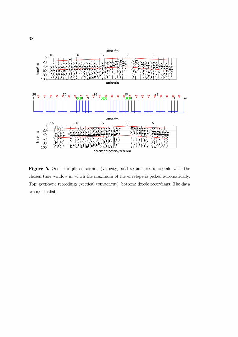
In order to pick the maximum amplitude of the signal, we define a time-window
in which we automatically detect the maximum of the envelope of the first
arrival on every trace. The time-window is defined on the seismoelectric signals
first, and the same time-window is used for the seismic records (see figure 5).
For a reason that we could not explain, the first arrival of the seismoelectric
signals is recorded before the first arrival of the seismic records, in the filtered
Page 19
18
data (figure 5) as well as in the raw data (figure 3). Such a feature is not usual.
Therefore we compared the time-response of our geophones to the time-response
of several other geophones, and we checked the band-pass filter of our geophones,
but could not find any explanation to this time delay. This phenomenon was
not encountered in other seismoelectric measurements done before by one of
the authors (Strahser 2007). It cannot be explained by spatial offsets
between electrodes and geophones. If we assume a spatial offset of
10 cm and take the typical velocity of 1250 m/s, the temporal offset
would be 0.08 ms, while we observe temporal offsets of more than
10 ms. This would correspond to an offset of more than 10 m. Noisy
traces were excluded from the analysis, as well as traces with exceedingly high
or low amplitudes.Figure 5
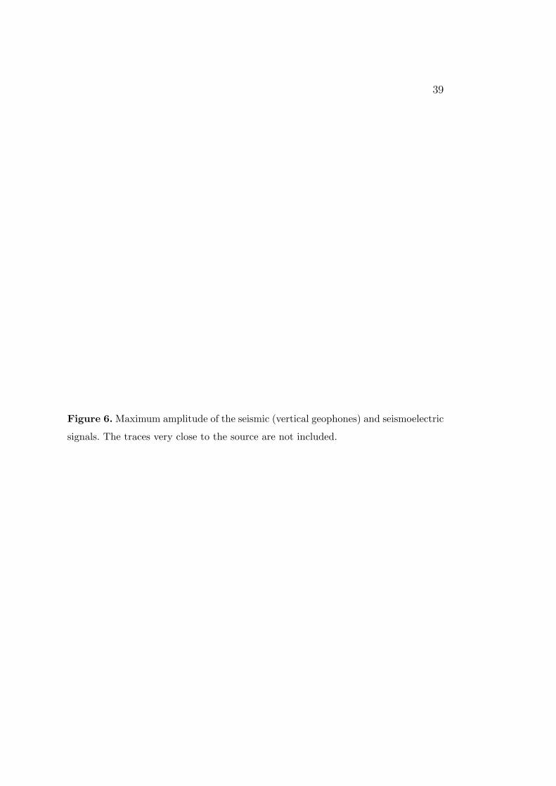
here. We plotted the maximum amplitude of the envelope of the seismic and
seismoelectric records as a function of the distance from the source in figure 6.
As expected, the (seismically induced) particle velocity decreases far from the
source. Therefore the induced seismoelectric signal decreases, too (see equation
5). Note that the seismoelectric signal is up to 0.8 mV/m near the source, and
only around 50 µV/m at 5 to 7 meters from the source. One can also see that
the summing up of two adjacent shots was not perfect here because there is a
clear zigzag pattern in the amplitudes.Figure 6
here. To study the seismoelectric transfer function between the electric field and
the acceleration, we have to normalize the seismoelectric data with respect to the
seismic data. We achieve this by plotting the amplitude of the seismoelectric
signal divided by the amplitude given by the geophone records (actually the
amplitude maximum within the time window as described in the beginning of
this section).
We also normalize the seismoelectric field with the vertical or horizontal seis-
Page 20
19
mic acceleration by taking the time derivative of the geophone records. These
two versions of the normalized seismoelectric field are plotted as a function of
the resistance of the dipole. The transfer function to calculate the grain veloc-
ity from the geophone voltage output was available for the vertical component
geophones, but not for the horizontal component geophones. It turned out that
these latter ones contained a different damping resistor than indicated in the
product specifications and that no transfer function was available for this exact
type of geophone. For that reason we calculated the mean of all recorded vertical
geophone maxima and the mean of all recorded horizontal geophone maxima.
The ratio was used to transfer the voltage output of the horizontal component
geophones to horizontal grain velocity using the transfer function for the ver-
tical component geophones. Although the the! ory shows that the horizontal
electrical field is proportional to the horizontal acceleration (see equation 5),
our results show that the highest data quality and the highest similarity with
the seismoelectric data can be found on the vertical velocity records. This is
not caused by the approximated transfer function of the horizontal component
geophones, since this function simply acts as a constant factor in the considered
frequency interval.
We automatically determine the time position of the maximum of the en-
velope for each seismic and each seismoelectric trace. If there is a difference of
more than 15 ms in these determined time positions between a seismic trace
and its corresponding seismoelectric trace, that trace is not taken into account
because in that case seismoelectric and seismic signals could be caused by differ-
ent phenomena than the theoretical coseismic electric signal caused by the the
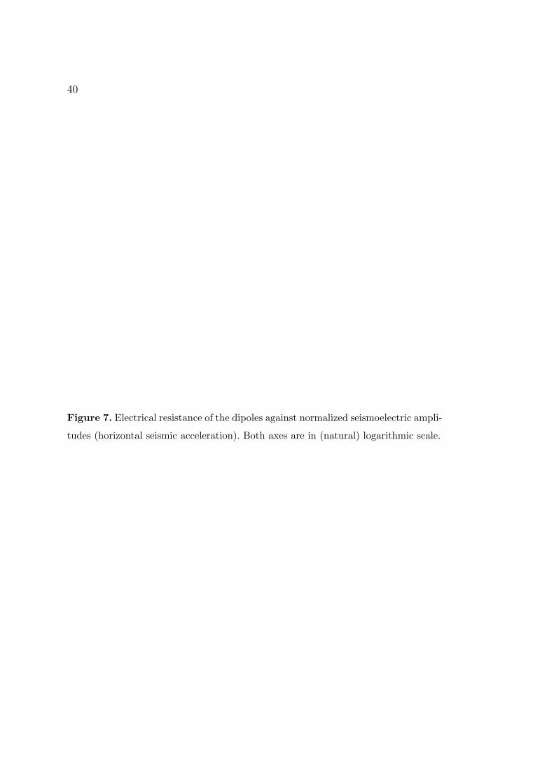
first arrivals of the compressional waves. In figure 7 we show the results for the
horizontal seismic acceleration, corresponding to 212 analyzed traces from both
fields (La Soutte and Champ du Feu). Most of the measurements are included in
Page 21
20
the range 2-12 kΩ and 50-1000 µV s2/m2. In order to quantify the seismoelectricFigure 7
here. amplitudes normalized with respect to the seismic amplitudes as a function of
the electrical resistance of the dipoles, we split the statistical study in seven re-
sistance intervals (figure 8). We fit the corresponding histogram distribution to
a normal law, and deduce an error on each mean value. The errors in normalized
amplitude and resistance are used as weights in the weighted linear regression.
Resistance regions with less amplitude scattering thus have a greater weight.
The regression line is found by minimizing deviations in normalized amplitudes
in an iterative manner such as described in e.g. ?).Figure 8
here. The resulting regression line and the corresponding equation are shown in
figure 9. Since the theory predicts that the horizontal electric field is propor-
tional to the horizontal acceleration (see equation 5), we will focus on this result.
The normalizations with the seismic vertical component and the seismic acceler-
ation are summed up in appendix A. They all show quite similar characteristics
and exponents in the regression equations, so the following discussion is largely
valid also for those data. Different numbers of resistance intervals yield slightly
different regression lines (again, see appendix A). These regression lines from
4, 5, and 7 resistance intervals are shown in figure 9a. We choose a resulting
regression line with large enough errors in dip and intercept to include the three
different regression lines from figure ??a (see figure 9b). The resulting relation
between resistance and the normalized seismoelectric amplitudes isFigure 9
here.RH,der = 0.12(±0.19)
(EH
uH
)−2.4(±1.4)
(11)
Page 22
21
5 DISCUSSION
Our analysis shows the following relation between the horizontal seismoelectric
field measured between two electrodes, the horizontal acceleration measured in
the middle of the dipole, and the electrical resistance R measured between the
electrodes:
EH
uH
∝ R−1/(2.4±1.4) ' R−0.42±0.25. (12)
During the measurements, the soil was usually quite humid at the surface so
that the contact resistance between electrode and soil was quite low. Therefore,
the measured resistance R is approximately proportional to the resistivity ρr.
The resistivity depends on the water saturation Sw as follows (Archie 1942):
ρr =ρf
φmSnw
, (13)
where ρf is the fluid resistivity, φ the porosity, and m and n the Archie expo-
nents (also called cementation exponent and saturation exponent, respectively).
Assuming that the porosity and the fluid resistivity are constant, the resistivity
is inversely proportional to the water saturation. The electrokinetic coefficient
is zero below a residual water saturation Sr, so that it is often described as a
function of the effective water saturation
Se =Sw − Sr
1− Sr
. (14)
This would involve, using equations 5, 6, 12, and 13:
Cs ∝ EH
uH
∝ ρ−0.42±0.25r ∝ S(0.42±0.25)n
e . (15)
Page 23
22
Assuming an electrokinetic coefficient at full water saturation as in equation
6, we propose that the electrokinetic coefficient depends on water saturation as:
Cs =ε ζ
η σf
S(0.42±0.25)ne . (16)
The results of our field study on the seismoelectric amplitude show that the
electrokinetic coefficient should increase with water saturation. A laboratory
study by Guichet et al. (2003) showed also an increase of the electrokinetic
coefficient with water saturation, and some models (Perrier & Morat 2000; Revil
et al. 2007) proposed an increase of this coefficient, too, but a precise power-
law versus water saturation is still in debate. We could hope to expect a
common behaviour in porous media without clays or carbonates.
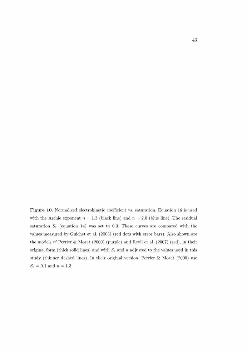
The saturation index n was observed to be about 2 for consolidated rocks and
to range from 1.3 to 2 for unconsolidated sands (Schon 1996; Guichet et al. 2003;
Lesmes & Friedman 2005). In figure 10, we apply equation 16 with n = 1.3 and
n = 2.0 and compare these curves with the normalized electrokinetic coefficients
measured by Guichet et al. (2003). The residual saturation Sr (equation 14) was
set to 0.3 as determined in a laboratory drainage experiment in a sand column
(Allegre et al. 2010). Our study leads to an electrokinetic coefficient dependence
on saturation as S0.55e to S0.84
e (for n = 1.3 and n = 2.0, respectively). The
experimental measurements of Guichet et al. (2003) have to be compared to
the empirical law using n=1.3 since this experimental study has been performed
on sand. A reasonable match between this experimental study and our results
can be seen. Also shown are the models of Perrier & Morat (2000) and! Revil
et al. (2007) (see appendix B for more descriptions). Since they use different
values for the residual saturation (Sr = 0.1 and Sr = 0.2, respectively) and n
(n = 1.0 in Revil et al. 2007), we add their models with Sr = 0.3 and n = 1.3
as used in this study, as well. The original version of Perrier & Morat (2000)
Page 24
23
is closest to the measured values of Guichet et al. (2003) but they used a very
low Sr value of 0.1. The tendency of the remaining curves is the same, with
our curve for n = 1.3 and the curve of Perrier & Morat (2000) for Sr = 0.3
being slightly closer to the values of Guichet et al. (2003) than the others.
These models were determined with different methods: Perrier & Morat (2000)
postulate their model, Guichet et al. (2003) performed laboratory experiments
of the streaming potential, the study of Revil et al. (2007) is a theoretical
one with laboratory experiments for comparison, and we derive the normalized
electrokinetic coefficient with seismoelectric field measurements. Keeping this
in mind, the match between the different curves is quite good. However we
note that in presence of clays or carbonates this behaviour may be
more complex. Finally we show that in the low frequency domain, taking into Figure 10
here.account the water saturation, the seismoelectric field and the seismic field are
related as:
E ' ε ζ
η σf
S(0.42±0.25)ne df u. (17)
6 CONCLUSION
We show through field measurements that seismoelectric signals were affected
by water content. Taking into account the water saturation and assuming the
Archie law for the resistivity in non-saturated conditions, the normalized seis-
moelectric field is a power-law of the effective saturation with the exponent
(0.42± 0.25)n, where n is Archie’s saturation exponent (see equation 17). Fur-
Page 25
24
ther studies are needed to improve our understanding of these phenomena. The
electrical resistance investigated in this study was restricted to relatively low
values such as 5-20 kΩ, corresponding to a relatively high water saturation. A
complementary study with higher values of resistance would improve our re-
sults and a comparison with detailed laboratory experiments should improve
our understanding of these phenomena.
7 ACKNOWLEDGMENTS
This work was supported by the French National Scientific Research Center
(CNRS), the Institut National des Sciences de l’Univers (INSU) through the
PNRH program, by the Alsace Region Research Network in Environmental Sci-
ences and Engineering (REALISE), and the Alsace Region. The postdoctoral
position for M. Strahser was funded by the Universite Louis Pasteur de Stras-
bourg (now part of Universite de Strasbourg). We are grateful to G. Herquel
and J.-B. Edel for helpful discussions and to C. Muller (GNS Science, Welling-
ton) for helpful discussions and the implementation of the sinusoid filter code
in Seismic Unix.
Page 26
25
REFERENCES
Adam, E. & Langlois, P., 1995. Elimination of monofrequency noise from seismic
records, Lithoprobe Seismic Processing Facility Newsletter , 8, 59–65.
Adamson, A. W., 1976. Physical chemistry of surfaces, John Wiley and sons, New
York.
Adler, P. M., Thovert, J. F., Jacquin, C., Morat, P., & Le Mouel, J. L., 1997.
Electrical signals induced by the atmospheric pressure variations in unsaturated
media, C.R. Acad. Sci. Paris, 324, 711–718.
Ageeva, O. A., Svetov, B. S., Sherman, G. K., & Shipulin, V., 1999. E-effect in
rocks, Russian Geology and Geophysics, 64, 1349–1356.
Allegre, V., Jouniaux, L., Lehmann, F., & Sailhac, P., 2010. Streaming Potential
dependence on water-content in fontainebleau sand, Geophys. J. Int., 182, 1248–
1266.
Archie, G. E., 1942. The electrical resistivity log as an aid in determining some
reservoir characteristics, Trans. Am. Inst. Min. Metall. Pet. Eng., (146), 54–62.
Aubert, M. & Atangana, Q. Y., 1996. Self-potential method in hydrogeological
exploration of volcanic areas, Ground Water , 34, 1010–1016.
Beamish, D., 1999. Characteristics of near surface electrokinetic coupling, Geophys.
J. Int., 137, 231–242.
Biot, M. A., 1956. Theory of propagation of elastic waves in a fluid-saturated porous
solid: I. low frequency range, J. Acoust. Soc. Am., 28(2), 168–178.
Block, G. I. & Harris, J. G., 2006. Conductivity dependence of seismoelectric wave
phenomena in fluid-saturated sediments, J. Geophys. Res., 111, B01304.
Bordes, C., Jouniaux, L., Dietrich, M., Pozzi, J.-P., & Garambois, S., 2006. First lab-
oratory measurements of seismo-magnetic conversions in fluid-filled Fontainebleau
sand, Geophys. Res. Lett., 33, L01302.
Bordes, C., Jouniaux, L., Garambois, S., Dietrich, M., Pozzi, J.-P., & Gaffet, S.,
2008. Evidence of the theoretically predicted seismo-magnetic conversion, Geophys.
J. Int., 174, 489–504.
Butler, K., 1996. Seismoelectrics effects of electrokinetic origin, PhS Thesis, Univ.
B.C. Vancouver, Canada.
Butler, K. E. & Russell, R. D., 1993. Substraction of powerline harmonics from
geophysical records, Geophysics, 58, 898–903.
Butler, K. E. & Russell, R. D., 2003. Cancellation of multiple harmonic noise series
Page 27
26
in geophysical records, Geophysics, 68, 1083–1090.
Chandler, R., 1981. Transient streaming potential measurements on fluid-saturated
porous structures: An experimental verification of Biot’s slow wave in the quasi-
static limit, J. Acoust. Soc. Am., 70, 116–121.
Chen, B. & Mu, Y., 2005. Experimental studies of seismoelectric effects in fluid-
saturated porous media, J. Geophys. Eng., 2, 222–230.
Cooke, C. E., 1955. Study of electrokinetic effects using sinusoidal pressure and
voltage, J. Chem. Phys., (23), 2299–2303.
Darnet, M. & Marquis, G., 2004. Modelling streaming potential (sp) signals induced
by water movement in the vadose zone, J. Hydrol., 285, 114–124.
Davis, J. A., James, R. O., & Leckie, J., 1978. Surface ionization and complexation
at the oxide/water interface, J. Colloid Interface Sci., 63, 480–499.
Dullien, F., 1992. Porous media: fluid transport and pore structure, Academic Press,
San Diego.
Dupuis, J. C. & Butler, K. E., 2006. Vertical seismoelectric profiling in a borehole
penetrating glaciofluvial sediments, Geophys. Res. Lett., 33.
Dupuis, J. C., Butler, K. E., & Kepic, A. W., 2007. Seismoelectric imaging of the
vadose zone of a sand aquifer, Geophysics, 72, A81–A85.
Dupuis, J. C., Butler, K. E., Kepic, A. W., & Harris, B. D., 2009. Anatomy of
a seismoelectric conversion: Measurements and conceptual modeling in boreholes
penetrating a sandy aquifer, J. Geophys. Res. Solid Earth, 114, B10306–+.
Garambois, S. & Dietrich, M., 2001. Seismoelectric wave conversions in porous
media: Field measurements and transfer function analysis, Geophysics, 66, 1417–
1430.
Garambois, S. & Dietrich, M., 2002. Full waveform numerical simulations of seis-
moelectromagnetic wave conversions in fluid-saturated stratified porous media, J.
Geophys. Res., 107(B7), ESE 5–1.
Gibert, D. & Pessel, M., 2001. Identification of sources of potential fields with the
continuous wavelet transform: Application to self-potential profiles, Geophys. Res.
Lett., 28, 1863–1866.
Gorsy, P., Hulin, G., Knobel, P., Sanchez, O., Thiebaut, C., Valois, R., & Wawrzy-
niak, P., 2006. Rapport de synthese, Champ du Feu, rapport de stage, Ecole et
Observatoire des Sciences de la Terre, Universite Louis Pasteur de Strasbourg, pp.
1–39.
Page 28
27
Guichet, X. & Zuddas, P., 2003. Effect of secondary minerals on electrokinetic
phenomena during water-rock intercation, Geophys. Res. Lett., 30, 1714.
Guichet, X., Jouniaux, L., & Pozzi, J.-P., 2003. Streaming potential of a sand column
in partial saturation conditions, J. Geophys. Res., 108(B3), 2141.
Guichet, X., Jouniaux, L., & Catel, N., 2006. Modification of streaming potential
by precipitation of calcite in a sand-water system: laboratory measurements in the
pH range from 4 to 12, Geophys. J. Int., 166, 445–460.
Haartsen, M. W. & Pride, S., 1997. Electroseismic waves from point sources in
layered media, J. Geophys. Res., 102, 24,745–24,769.
Haartsen, M. W., Dong, W., & Toksoz, M. N., 1998. Dynamic streaming currents
from seismic point sources in homogeneous poroelastic media, Geophys. J. Int.,
132, 256–274.
Haines, S. S., Guitton, A., & Biondi, B., 2007a. Seismoelectric data processing for
surface surveys of shallow targets, Geophysics, 72, G1–G8.
Haines, S. S., Pride, S. R., Klemperer, S. L., & Biondi, B., 2007b. Seismoelectric
imaging of shallow targets, Geophysics, 72, G9–G20.
Henry, P., Jouniaux, L., Screaton, E. J., S.Hunze, & Saffer, D. M., 2003. Anisotropy
of electrical conductivity record of initial strain at the toe of the Nankai accre-
tionary wedge, J. Geophys. Res., 108, 2407.
Hunt, C. W. & Worthington, M. H., 2000. Borehole elektrokinetic responses in frac-
ture dominated hydraulically conductive zones, Geophys. Res. Lett., 27(9), 1315–
1318.
Hunter, R., 1981. Zeta Potential in Colloid Science: Principles and Applications,
Academic., New York.
Ishido, T. & Mizutani, H., 1981. Experimental and theoretical basis of electrokinetic
phenomena in rock water systems and its applications to geophysics, J. Geophys.
Res., 86, 1763–1775.
Jaafar, M. Z., Vinogradov, J., & Jackson, M. D., 2009. Measurement of streaming
potential coupling coefficient in sandstones saturated with high salinity nacl brine,
Geophys. Res. Lett., 36.
Jouniaux, L., Lallemant, S., & Pozzi, J., 1994. Changes in the permeability, stream-
ing potential and resistivity of a claystone from the Nankai prism under stress,
Geophys. Res. Lett., 21, 149–152.
Jouniaux, L., Pozzi, J.-P., Berthier, J., & Masse, P., 1999. Detection of fluid flow
Page 29
28
variations at the Nankai trough by electric and magnetic measurements in boreholes
or at the seafloor, J. Geophys. Res., 104, 29293–29309.
Jouniaux, L., Bernard, M.-L., Zamora, M., & Pozzi, J.-P., 2000. Streaming potential
in volcanic rocks from Mount Pelee, J. Geophys. Res., 105, 8391–8401.
Jouniaux, L., Zamora, M., & Reuschle, T., 2006. Electrical conductivity evolution of
non-saturated carbonate rocks during deformation up to failure, Geophys. J. Int.,
167, 1017–1026.
Lesmes, D. P. & Friedman, S. P., 2005. Relationships between the electrical and
hydrogeological properties of rocks and soils, Hydrogeophysics, chap. 4, pp. 87–
128, eds Rubin, Y. & Hubbard, S. S., Springer, Dordrecht, The Netherlands.
Long, L. T. & Rivers, W. K., 1975. Field measurement of the electroseismic response,
Geophysics, 40, 233–245.
Lorne, B., Perrier, F., & Avouac, J.-P., 1999. Streaming potential measurements.
1. properties of the electrical double layer from crushed rock samples, J. Geophys.
Res., 104(B8), 17,857–17,877.
Maineult, A., Strobach, E., & Renner, J., 2008. Self-potential signals induced by
periodic pumping, J. Geophys. Res., 113, B01203.
Martner, S. T. & Sparks, N. R., 1959. The electroseismic effect, Geophysics, 24(2),
297–308.
Mironov, S. A., Parkhomenko, E. I., & Chernyak, G. Y., 1994. Seismoelectric effect
in rocks containing gas or fluid hydrocarbon (english translation), Izv. Phys. Solid
Earth, 29(11).
Packard, R. G., 1953. Streaming potentials across capillaries for sinusoidal pressure,
J. Chem. Phys, 1(21), 303–307.
Parkhomenko, E. & Gaskarov, I., 1971. Borehole and laboratory studies of the
seismoelectric effect of the second kind in rocks, Izv. Akad. Sci. USSR, Physics
Solid Earth, 9, 663–666.
Parkhomenko, I. & Tsze-San, C., 1964. A study of the influence of moisture on
the magnitude of the seismoelectric effect in sedimentary rocks by a laboratory
method, Bull. (Izv.) Acad. Sci., USSR, Geophys. Ser., pp. 115–118.
Perrier, F. & Morat, P., 2000. Characterization of electrical daily variations induced
by capillary flow in the non-saturated zone, Pure Appl. Geophys., 157, 785–810.
Perrier, F., Trique, M., Lorne, B., Avouac, J.-P., Hautot, S., & Tarits, P., 1998.
Electric potential variations associated with lake variations, Geophys. Res. Lett.,
Page 30
29
25, 1955–1958.
Pinettes, P., Bernard, P., Cornet, F., Hovhannissian, G., Jouniaux, L., Pozzi, J.-P.,
& Barthes, V., 2002. On the difficulty of detecting streaming potentials generated
at depth, Pure Appl. Geophys., 159, 2629–2657.
Pozzi, J.-P. & Jouniaux, L., 1994. Electrical effects of fluid circulation in sediments
and seismic prediction, C.R. Acad. Sci. Paris, serie II , 318(1), 73–77.
Pride, S., 1994. Governing equations for the coupled electromagnetics and acoustics
of porous media, Phys. Rev. B: Condens. Matter , 50, 15678–15695.
Reppert, P. & Morgan, F., 2003a. Temperature-dependent streaming potentials: 1.
theory, J. Geophys. Res., 108, 2546.
Reppert, P. & Morgan, F., 2003b. Temperature-dependent streaming potentials: 2.
laboratory, J. Geophys. Res., 108, 2547.
Reppert, P. M., Morgan, F. D., Lesmes, D. P., & Jouniaux, L., 2001. Frequency-
dependent streaming potentials, J. Colloid Interface Sci., (234), 194–203.
Revil, A., Linde, N., Cerepi, A., Jougnot, D., Matthai, S., & Finsterle, S., 2007.
Electrokinetic coupling in unsaturated porous media, J. Colloid Interface Sci.,
313, 315–327.
Sailhac, P., Darnet, M., & Marquis, G., 2004. Electrical streaming potential mea-
sured at the ground surface: forward modeling and inversion issues for monitoring
infiltration and characterizing the vadose zone, Vadose Zone J., (3), 1200–1206.
Sailhac, P., Bano, M., Behaegel, M., Girard, J.-F., Para, F., Ledo, J., Marquis, G.,
Matthey, P.-D., & Ramirez, J.-O., 2009. Characterizing vadose zone and perched
aquifer near Vosgian ridges in La Soutte experimental site, Obernai, France, C.R.
Geosci., 341, 818–830.
Saracco, G., Labazuy, P., & Moreau, F., 2004. Localization of self-potential sources
in volcano-electric effect with complex continuous wavelet transform and electrical
tomography methods for an active volcano, Geophys. Res. Lett., (31), L12610.
Saunders, J. H., Jackson, M. D., & Pain, C. C., 2006. A new numerical model of
electrokinetic potential response during hydrocarbon recovery, Geophys. Res. Lett.,
33, L15316.
Schoemaker, F., Smeulders, D., & Slob, E., 2008. Electrokinetic effect: Theory and
measurement, SEG Technical Program Expanded Abstracts, pp. 1645–1649.
Schon, J., 1996. Physical properties of rocks - fundamentals and principles of petro-
physics, vol. 18, Elsevier Science Ltd., Handbook of Geophysical Exploration, Seis-
Page 31
30
mic exploration.
Sill, W., 1983. Self-potential modeling from primary flows, Geophysics, 48, 76–86.
Strahser, M. H. P., 2007. Near surface seismoelectrics in comparative field studies,
PhD Thesis, Christian-Albrechts-Universitat zu Kiel, Germany.
Strahser, M. H. P., Rabbel, W., & Schildknecht, F., 2007. Polarisation and slowness
of seismoelectric signals: a case study, Near Surface Geophysics, 5, 97–114.
Thompson, A., Hornbostel, S., Burns, J., Murray, T., Raschke, R., Wride, J., Mc-
Cammon, P., Sumner, J., Haake, G., Bixby, M., Ross, W., White, B., Zhou, M., &
Peczak, P., 2005. Field tests of electroseismic hydrocarbon detection, SEG Tech-
nical Program Expanded Abstracts.
Thompson, A., Sumner, J., & Hornbostel, S., 2007. Electromagnetic-to-seismic con-
version: A new direct hydrocarbon indicator, The Leading Edge, pp. 428–435.
Thompson, R. R., 1936. The seismic-electric effect, Geophysics, 1(3), 327–335.
Zhu, Z. & Toksoz, M. N., 2003. Crosshole seismoelectric measurements in borehole
models with fractures, Geophysics, 68(5), 1519–1524.
Zhu, Z., Haartsen, M. W., & Toksoz, M. N., 1999. Experimental studies of electroki-
netic conversions in fluid-saturated borehole models, Geophysics, 64, 1349–1356.
Page 32
31
LIST OF FIGURES
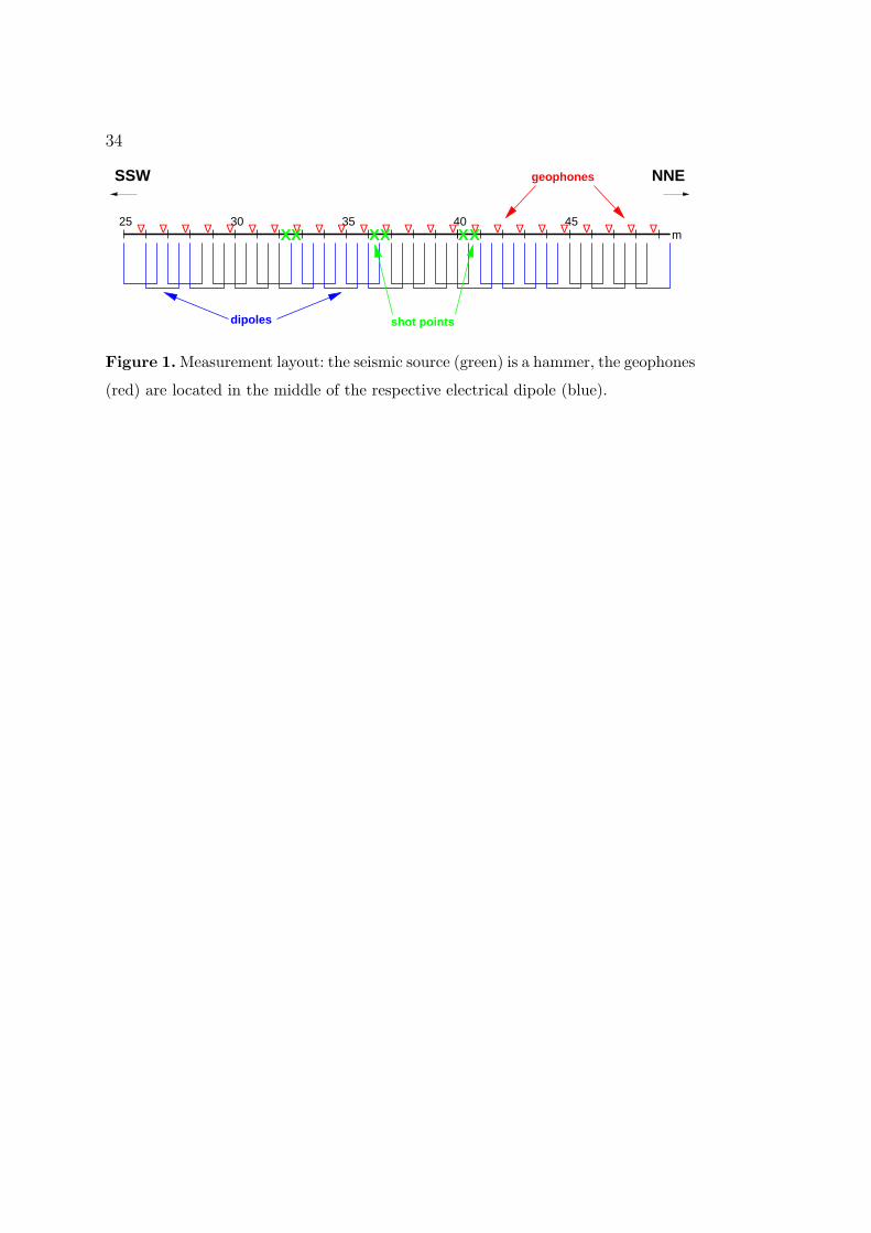
1 Measurement layout: the seismic source (green) is a hammer, the
geophones (red) are located in the middle of the respective electrical
dipole (blue).
2 The amount of traces can be doubled by adding the traces of
two adjacent shotpoints, in this case yielding dipole distances of 0.5
m. The traces from the first shotpoint are in red, the traces from the
second one in black.
3 Seismoelectric and seismic signals measured along the profile at
La Soutte (raw data). The shot point is located at distance zero. Top:
geophone recordings (vertical component), middle: measurement lay-
out (see annotations in figure 1), bottom: dipole recordings. The data
are agc-scaled. Noisy traces were discarded from the records.
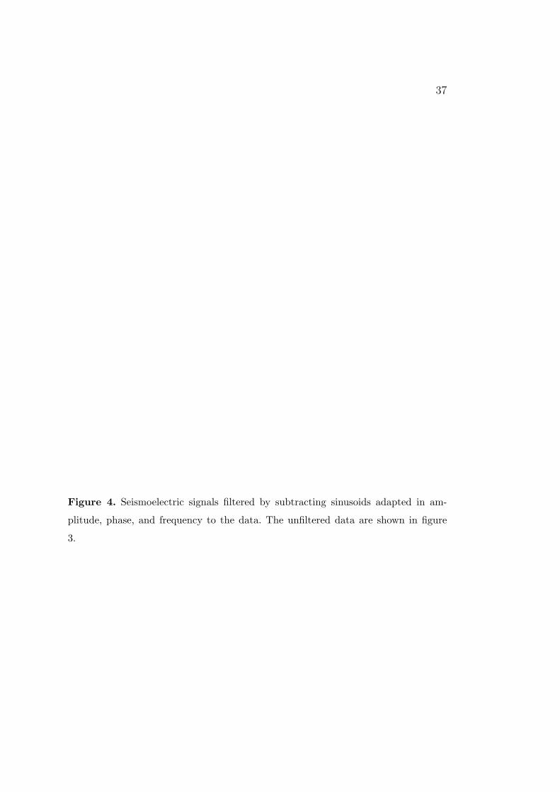
4 Seismoelectric signals filtered by subtracting sinusoids adapted
in amplitude, phase, and frequency to the data. The unfiltered data
are shown in figure 3.
5 One example of seismic (velocity) and seismoelectric signals with
the chosen time window in which the maximum of the envelope is
picked automatically. Top: geophone recordings (vertical component),
bottom: dipole recordings. The data are agc-scaled.
6 Maximum amplitude of the seismic (vertical geophones) and seis-
moelectric signals. The traces very close to the source are not included.
7 Electrical resistance of the dipoles against normalized seismo-
electric amplitudes (horizontal seismic acceleration). Both axes are in
(natural) logarithmic scale.
Page 33
32
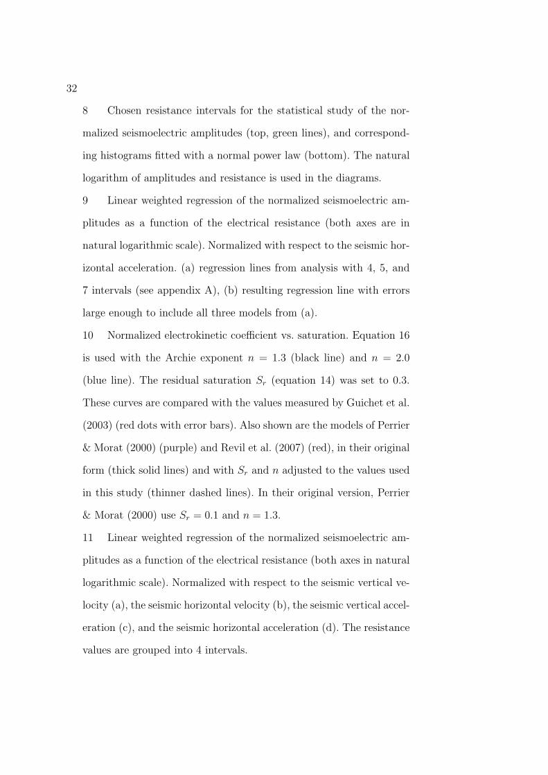
8 Chosen resistance intervals for the statistical study of the nor-
malized seismoelectric amplitudes (top, green lines), and correspond-
ing histograms fitted with a normal power law (bottom). The natural
logarithm of amplitudes and resistance is used in the diagrams.
9 Linear weighted regression of the normalized seismoelectric am-
plitudes as a function of the electrical resistance (both axes are in
natural logarithmic scale). Normalized with respect to the seismic hor-
izontal acceleration. (a) regression lines from analysis with 4, 5, and
7 intervals (see appendix A), (b) resulting regression line with errors
large enough to include all three models from (a).
10 Normalized electrokinetic coefficient vs. saturation. Equation 16
is used with the Archie exponent n = 1.3 (black line) and n = 2.0
(blue line). The residual saturation Sr (equation 14) was set to 0.3.
These curves are compared with the values measured by Guichet et al.
(2003) (red dots with error bars). Also shown are the models of Perrier
& Morat (2000) (purple) and Revil et al. (2007) (red), in their original
form (thick solid lines) and with Sr and n adjusted to the values used
in this study (thinner dashed lines). In their original version, Perrier
& Morat (2000) use Sr = 0.1 and n = 1.3.
11 Linear weighted regression of the normalized seismoelectric am-
plitudes as a function of the electrical resistance (both axes in natural
logarithmic scale). Normalized with respect to the seismic vertical ve-
locity (a), the seismic horizontal velocity (b), the seismic vertical accel-
eration (c), and the seismic horizontal acceleration (d). The resistance
values are grouped into 4 intervals.
Page 34
33
12 Linear weighted regression of the normalized seismoelectric am-
plitudes as a function of the electrical resistance (both axes in natural
logarithmic scale). Normalized with respect to the seismic vertical ve-
locity (a), the seismic horizontal velocity (b), the seismic vertical accel-
eration (c), and the seismic horizontal acceleration (d). The resistance
values are grouped into 5 intervals.
13 Linear weighted regression of the normalized seismoelectric am-
plitudes as a function of the electrical resistance (both axes in natural
logarithmic scale). Normalized with respect to the seismic vertical ve-
locity (a), the seismic horizontal velocity (b), the seismic vertical accel-
eration (c), and the seismic horizontal acceleration (d). The resistance
values are grouped into 7 intervals.
Page 35
34
25 3530 40 45m
∆ ∆ ∆ ∆ ∆ ∆ ∆ ∆ ∆ ∆ ∆ ∆ ∆ ∆ ∆ ∆ ∆ ∆ ∆ ∆ ∆ ∆ ∆ ∆
XX XX XX
dipoles
SSW NNEgeophones
shot points
Figure 1. Measurement layout: the seismic source (green) is a hammer, the geophones
(red) are located in the middle of the respective electrical dipole (blue).
Page 36
35
Figure 2. The amount of traces can be doubled by adding the traces of two adjacent
shotpoints, in this case yielding dipole distances of 0.5 m. The traces from the first
shotpoint are in red, the traces from the second one in black.
Page 37
36
020406080
100
time/
ms
-15 -10 -5 0 5offset/m
seismic
25 3530 40 45m
∆ ∆ ∆ ∆ ∆ ∆ ∆ ∆ ∆ ∆ ∆ ∆ ∆ ∆ ∆ ∆ ∆ ∆ ∆ ∆ ∆ ∆ ∆ ∆
XX XX XX
020406080
100
time/
ms
-15 -10 -5 0 5offset/m
seismoelectric, unfiltered
Figure 3. Seismoelectric and seismic signals measured along the profile at La Soutte
(raw data). The shot point is located at distance zero. Top: geophone recordings
(vertical component), middle: measurement layout (see annotations in figure 1), bot-
tom: dipole recordings. The data are agc-scaled. Noisy traces were discarded from the
records.
Page 38
37
Figure 4. Seismoelectric signals filtered by subtracting sinusoids adapted in am-
plitude, phase, and frequency to the data. The unfiltered data are shown in figure
3.
Page 39
38
020406080
100
time/
ms
-15 -10 -5 0 5offset/m
seismic
25 3530 40 45m
∆ ∆ ∆ ∆ ∆ ∆ ∆ ∆ ∆ ∆ ∆ ∆ ∆ ∆ ∆ ∆ ∆ ∆ ∆ ∆ ∆ ∆ ∆ ∆
XX XX XX
020406080
100
time/
ms
-15 -10 -5 0 5offset/m
seismoelectric, filtered
Figure 5. One example of seismic (velocity) and seismoelectric signals with the
chosen time window in which the maximum of the envelope is picked automatically.
Top: geophone recordings (vertical component), bottom: dipole recordings. The data
are agc-scaled.
Page 40
39
Figure 6. Maximum amplitude of the seismic (vertical geophones) and seismoelectric
signals. The traces very close to the source are not included.
Page 41
40
Figure 7. Electrical resistance of the dipoles against normalized seismoelectric ampli-
tudes (horizontal seismic acceleration). Both axes are in (natural) logarithmic scale.
Page 42
41
Figure 8. Chosen resistance intervals for the statistical study of the normalized
seismoelectric amplitudes (top, green lines), and corresponding histograms fitted with
a normal power law (bottom). The natural logarithm of amplitudes and resistance is
used in the diagrams.
Page 43
42
Figure 9. Linear weighted regression of the normalized seismoelectric amplitudes as
a function of the electrical resistance (both axes are in natural logarithmic scale).
Normalized with respect to the seismic horizontal acceleration. (a) regression lines
from analysis with 4, 5, and 7 intervals (see appendix A), (b) resulting regression line
with errors large enough to include all three models from (a).
Page 44
43
Figure 10. Normalized electrokinetic coefficient vs. saturation. Equation 16 is used
with the Archie exponent n = 1.3 (black line) and n = 2.0 (blue line). The residual
saturation Sr (equation 14) was set to 0.3. These curves are compared with the
values measured by Guichet et al. (2003) (red dots with error bars). Also shown are
the models of Perrier & Morat (2000) (purple) and Revil et al. (2007) (red), in their
original form (thick solid lines) and with Sr and n adjusted to the values used in this
study (thinner dashed lines). In their original version, Perrier & Morat (2000) use
Sr = 0.1 and n = 1.3.
Page 45
44
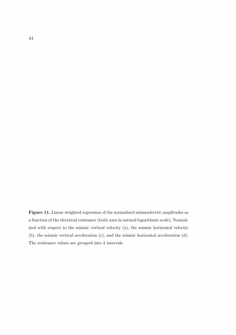
Figure 11. Linear weighted regression of the normalized seismoelectric amplitudes as
a function of the electrical resistance (both axes in natural logarithmic scale). Normal-
ized with respect to the seismic vertical velocity (a), the seismic horizontal velocity
(b), the seismic vertical acceleration (c), and the seismic horizontal acceleration (d).
The resistance values are grouped into 4 intervals.
Page 46
45
Figure 12. Linear weighted regression of the normalized seismoelectric amplitudes as
a function of the electrical resistance (both axes in natural logarithmic scale). Normal-
ized with respect to the seismic vertical velocity (a), the seismic horizontal velocity
(b), the seismic vertical acceleration (c), and the seismic horizontal acceleration (d).
The resistance values are grouped into 5 intervals.
Page 47
46
Figure 13. Linear weighted regression of the normalized seismoelectric amplitudes as
a function of the electrical resistance (both axes in natural logarithmic scale). Normal-
ized with respect to the seismic vertical velocity (a), the seismic horizontal velocity
(b), the seismic vertical acceleration (c), and the seismic horizontal acceleration (d).
The resistance values are grouped into 7 intervals.
Page 48
47
APPENDIX A: REGRESSION RESULTS FOR DIFFERENT
INTERVAL NUMBERS
In figure 9, we presented a linear weighted regression of the normalized seismo-
electric amplitudes as a function of the electrical resistance. Since it is necessary
to have a uniform sampling for a regression in log-log scale, we subdivided the
range of the measured resistivities into several intervals. Different numbers of
intervals yield slightly different regression lines. We show here the results of a
weighted least squares regression for 4, 5, and 7 intervals (figures 11, 12, and 13,
respectively). This gives us an indication of the uncertainties of the final result.
The seismoelectric data (horizontal component) are normalized with respect to
seismic data in four versions: the seismic vertical and horizontal components
and in each case the original form of the data (velocity) and the first deriva-
tive in time (acceleration). As explained in section ??, Garambois & Dietrich
(2001) showed that the seismoelectric (coseismic) signal is proportional to the
ground acceleration, i.e. the time derivative of the horizontal geophone output.
However, we analyze all four possible combinations here since field observations
sometimes showed a greater similarity between the seismoelectric horizontal
component and the seismic vertical component, often in the non-derived form.
Figure 11
here.Figure 12
here.Figure 13
here.
In general, the regression lines of the different interval models do not differ
much. As explained in section 4.2, it is mainly the exponent of the regression
equation that we are interested in. We follow a careful approach and choose
to incorporate the results of all three models with different intervals into the
exponent which gives us EH/uV ∝ R−1/(2.0±0.9) ' R−0.49±0.21for normaliza-
tion with the vertical seismic component, EH/uH ∝ R−1/(2.7±2.5) ' R−0.37±0.34
with the horizontal seismic component, EH/uV ∝ R−1/(1.7±0.6) ' R−0.58±0.21
with the time-derived vertical seismic component, and EH/uH ∝ R−1/(2.4±1.4) '
Page 49
48
R−0.42±0.25 with the time-derived horizontal seismic component. In section 5, we
refer to the seismoelectric amplitudes normalized with the time-derived hori-
zontal seismic amplitudes but as can be seen, ! the other exponents are quite
similar, so the discussion is largely valid also for those data.
APPENDIX B: MODELS OF PERRIER & MORAT (2000) AND
REVIL ET AL. (2007)
In figure 10 we compare the behavior of the normalized electrokinetic coefficient
against saturation as predicted by our experimentally derived law (equation 15)
with two other models proposed in literature. Perrier & Morat (2000) suggest
(in the notation used in this present article)
Cs
C0s
=S2
e
Snw
, (B.1)
with C0s : electrokinetic coefficient at full saturation, and n: Archie’s satura-
tion exponent. These authors use n = 2. Following Adler et al. (1997) who cite
Dullien (1992), they set the residual saturation to Sr = 0.1.
Revil et al. (2007) use
Cs
C0s
=S
(2+3λ)/λe
Sn+1w
, (B.2)
where λ is a curve-shape parameter corresponding to an index for the pore
space distribution. A typical value for sand is λ = 1.7. Also for sand, Revil et al.
(2007) use Sr = 0.2 and n = 1.0.