Dependency Reduction with Divisive Normalization ...lsw/papers/nc11.pdfDependency Reduction with...

LETTER Communicated by Odelia Schwartz

Dependency Reduction with Divisive Normalization:Justification and Effectiveness

Siwei [email protected] Science Department, University at Albany, State University of New York,Albany, NY 12222, U.S.A.

Efficient coding transforms that reduce or remove statistical dependenciesin natural sensory signals are important for both biology and engineer-ing. In recent years, divisive normalization (DN) has been advocated asa simple and effective nonlinear efficient coding transform. In this work,we first elaborate on the theoretical justification for DN as an efficientcoding transform. Specifically, we use the multivariate t model to rep-resent several important statistical properties of natural sensory signalsand show that DN approximates the optimal transforms that eliminatestatistical dependencies in the multivariate t model. Second, we showthat several forms of DN used in the literature are equivalent in theireffects as efficient coding transforms. Third, we provide a quantitativeevaluation of the overall dependency reduction performance of DN forboth the multivariate t models and natural sensory signals. Finally, wefind that statistical dependencies in the multivariate t model and natu-ral sensory signals are increased by the DN transform with low-inputdimensions. This implies that for DN to be an effective efficient codingtransform, it has to pool over a sufficiently large number of inputs.

1 Introduction

A central principle in the study of biological sensory systems is that theyare adapted to match the statistical properties of the sensory signals in thenatural environments to which they are exposed (Attneave, 1954). The effi-cient coding hypothesis (Barlow, 1961; Atick, 1992) further suggests that asensory system might be understood as a transform that reduces redundan-cies in the input stimuli. Such efficient coding transforms are of importancein both biology and engineering: the reduced redundancies in the neural re-sponses facilitate efficient representations of sensory input for ecologicallyrelevant tasks such as novelty detection and associative learning (Barlow,2001). In addition, with the reduced dependencies, sensory signals can bemore efficiently stored, transmitted, and processed.

Starting with the use of second-order decorrelation methods in explain-ing functional roles of photoreceptors and retinal ganglion cells (Atick &

Neural Computation 23, 2942–2973 (2011) c© 2011 Massachusetts Institute of Technology

Dependency Reduction with Divisive Normalization 2943

ilumits

)u( sesnopser

√

√α

denetihw

)x( esnopser

/+ u =x√

α+ x x

...........

...

...

Figure 1: A schematic illustration and the definition of the DN transform.

Redlich, 1992; Atick, Li, & Redlich, 1992; Ruderman, Cronin, & Chiao, 1998),studies in linear efficient coding transforms for natural sensory signals haveled to fruitful developments that culminate in the independent componentanalysis (ICA) methodology (Olshausen & Field, 1996; van der Schaaf & vanHateren, 1996; Bell & Sejnowski, 1997; Lewicki, 2002). These efforts werewidely lauded as a confirmation of the efficient coding hypothesis in thestudy of biological perception, as the obtained ICA basis functions closelyresemble the receptive fields of neurons in various cortex areas. In spite ofthese successes, early studies suggested that linear transforms may not beoptimal for reducing dependencies in natural sensory signals (Zetzsche &Barth, 1990; Baddeley, 1996; Zetzsche & Krieger, 1999), which were furtherconfirmed with observations of strong residual statistical dependencies af-ter ICA-like linear transforms (Wegmann & Zetzsche, 1990; Simoncelli &Buccigrossi, 1997) and quantitative evaluations that ICA achieves only amarginal improvement over principal component analysis (PCA) in reduc-ing statistical dependencies in natural images (Bethge, 2006). Indeed, thereare statistical dependencies in natural sensory signals that linear transformscannot reduce (Lyu & Simoncelli, 2009b; Eichhorn, Sinz, & Bethge, 2009).This motivates the search for effective nonlinear efficient coding transformsfor natural sensory signals.

Divisive normalization (DN) is a simple nonlinear efficient coding trans-form that recently has been widely studied (Schwartz & Simoncelli, 2001a;Valerio & Navarro, 2003a, 2003b; Malo & Laparra, 2010; Lyu, 2010). Thestandard form of DN transform we adopt in this work is illustrated schemat-ically in Figure 1. Here, x = (x1, . . . , xd )′ is a vector describing the responsesof input stimuli projected onto a set of front-end linear basis functions.These linear basis functions remove first- and second-order local statisti-cal dependencies and whiten the inputs so that they all have the sameweights when squared and pooled with a semisaturation constant α. Thesquare root of the pooling is divided from the response of each individ-ual linear basis function to obtain the final output of the DN transform,u = (u1, · · · , ud )′.

2944 S. Lyu

In this work, we first elaborate on the theoretical justification of DN asan efficient coding transform. Specifically, we use the multivariate t modelto represent several important statistical properties of natural sensory sig-nals and show that DN approximates the optimal transforms that eliminatestatistical dependencies in the multivariate t model. Second, using the multi-information as a quantitative measure of statistical dependency, we showthat several different forms of DN are equivalent in terms of dependencyreduction. Third, we provide a quantitative evaluation of the overall de-pendency reduction performance of DN for both the multivariate t modelsand natural sensory signals. Finally, we find that statistical dependencies inthe multivariate t model and natural sensory signals are increased by theDN transform with low input dimensions. This implies that for DN to bean effective and efficient coding transform, it has to pool over a sufficientlylarge number of inputs.

The rest of this article is organized as follows. After reviewing relevantprevious works in section 2, we describe in section 3 some basic statisticalproperties of natural sensory signals and demonstrate how these propertiescan be captured with the multivariate t model. In section 4, we show thatDN transform approximates the optimal efficient coding transforms for themultivariate t model. Sections 5 and 6 report the experimental evaluation ofthe effectiveness of the DN transform as an efficient coding transform for themultivariate t models and natural sensory signal data. Section 7 concludeswith discussion and future work. To make the description continuous, wedefer all formal proofs to the appendixes. (A preliminary version of thiswork has been presented in Lyu, 2010.)

2 Related Work

In biology, DN is a popular model for many nonlinear behaviors of neuralresponses that cannot be well described with the classical linear-nonlinearPoisson model (Chichilnisky, 2001; Pillow & Simoncelli, 2006). Such non-linearities can be found in the auditory (Schwartz & Simoncelli, 2001b)and the olfactory pathways (Olsen, Bhandawat, & Wilson, 2010), as wellas various stages of the visual pathway, including the retina (Shapley &Enroth-Cugell, 1984; Solomon, Lee, & Sun, 2006), the lateral geniculate nu-cleus (Mante, Bonin, & Carandini, 2008), the primary visual cortex (Heeger,1992; Rust, Schwartz, Movshon, & Simoncelli, 2005), and other extrastriatecortex, such as area MT (Simoncelli & Heeger, 1998) and area IT (Zoccolan,Cox, & DiCarlo, 2005). In low-level visual perception, DN has been relatedto various functional roles, including dynamic gain control (Shapley &Enroth-Cugell, 1984), decoding activities of neuronal populations (Deneve,Pouget, & Latham, 1999; Ringach, 2010), neural adaptation (Wainwright,Schwartz, & Simoncelli, 2002), and visual saliency (Gao & Vasconcelos,2009). It has also been used to account for high-level perceptual phenomenasuch as masking (Foley, 1994; Watson & Solomon, 1997) and attention (Lee


& Maunsell, 2009; Reynolds & Heeger, 2009). DN is believed to be imple-mentable with the cortical neurons (Carandini & Heeger, 1994; Carandini,Heeger, & Senn, 2002), though the specific neural mechanism for such animplementation is still under debate (see Holt & Koch, 1997).

Because of the prevalence of normalization-type behaviors in biologicalsensory systems, DN has become an integral component in theoretical mod-els describing information encoding of cortical neurons (Ringach, 2010). Inaddition, in engineering fields such as image processing and computer vi-sion, nonlinear image representations based on DN have been applied toimage compression (Malo, Epifanio, Navarro, & Simoncelli, 2006), contrastenhancement (Lyu & Simoncelli, 2008), image quality metrics (Li & Wang,2008; Laparra, Munoz-Mari, & Malo, 2010), and object recognition (Jarrett,Kavukcuoglu, Ranzato, & LeCun, 2009), all showing significant improve-ments in performance over linear representations.

In the context of efficient coding theory, the study in Brady and Field(2000) suggests that DN maximizes the entropy of each output componentto better use the channel capacity. Based on empirical observations, theseminal work of Schwartz and Simoncelli (2001a) proposes that DN is anonlinear efficient coding transform in biological perception that reducesstatistical dependencies in the input natural sensory signals. Subsequently,this hypothesis was tested in Valerio and Navarro (2003a, 2003b). How-ever, experiments in these works examined only pairwise dependencieswith mutual information estimated from histograms, a process prone tobiases due to the data binning procedure (Paninski, 2003). The more recentwork of Malo and Laparra (2010) uses a form of DN whose parameters areobtained from psychophysical experiments. While providing an interestingalternative perspective, this is only an indirect account for DN as an efficientcoding transform for natural sensory signals.

Recently a general methodology known as radial gaussianization (RG)has been shown to provide efficient coding transforms for sources withelliptical symmetric densities that capture local statistical dependencies ofnatural sensory signals (Lyu & Simoncelli, 2009b; Sinz & Bethge, 2009). Inthese studies, it has been shown that the transformation obtained by RGcan be closely approximated by DN. On the other hand, in spite of betterperformance in dependency reduction, the nonlinear transform obtainedfrom RG has not been fitted to data in biological sensory pathways.

3 Statistical Properties of Natural Sensory Signals andMultivariate t Model

Sensory signals in natural environments are highly structured and non-random. These regularities exhibit statistical properties that distinguishthem from the rest of the ensemble of all possible signals. Particularly, inthe bandpass-filtered domains constructed from various linear transformsconsisting of basis functions with localized support in space, frequency,

2946 S. Lyu

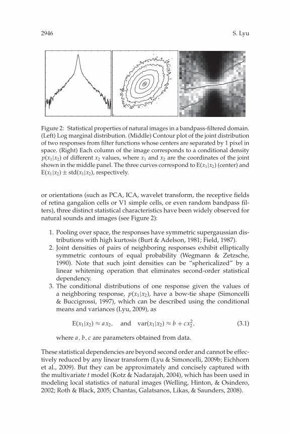
Figure 2: Statistical properties of natural images in a bandpass-filtered domain.(Left) Log marginal distribution. (Middle) Contour plot of the joint distributionof two responses from filter functions whose centers are separated by 1 pixel inspace. (Right) Each column of the image corresponds to a conditional densityp(x1|x2) of different x2 values, where x1 and x2 are the coordinates of the jointshown in the middle panel. The three curves correspond to E(x1|x2) (center) andE(x1|x2) ± std(x1|x2), respectively.

or orientations (such as PCA, ICA, wavelet transform, the receptive fieldsof retina gangalion cells or V1 simple cells, or even random bandpass fil-ters), three distinct statistical characteristics have been widely observed fornatural sounds and images (see Figure 2):

1. Pooling over space, the responses have symmetric supergaussian dis-tributions with high kurtosis (Burt & Adelson, 1981; Field, 1987).

2. Joint densities of pairs of neighboring responses exhibit ellipticallysymmetric contours of equal probability (Wegmann & Zetzsche,1990). Note that such joint densities can be “sphericalized” by alinear whitening operation that eliminates second-order statisticaldependency.

3. The conditional distributions of one response given the values ofa neighboring response, p(x1|x2), have a bow-tie shape (Simoncelli& Buccigrossi, 1997), which can be described using the conditionalmeans and variances (Lyu, 2009), as

E(x1|x2) ≈ ax2, and var(x1|x2) ≈ b + cx22 , (3.1)

where a , b, c are parameters obtained from data.

These statistical dependencies are beyond second order and cannot be effec-tively reduced by any linear transform (Lyu & Simoncelli, 2009b; Eichhornet al., 2009). But they can be approximately and concisely captured withthe multivariate t model (Kotz & Nadarajah, 2004), which has been used inmodeling local statistics of natural images (Welling, Hinton, & Osindero,2002; Roth & Black, 2005; Chantas, Galatsanos, Likas, & Saunders, 2008).


Figure 3: Properties of the multivariate t models. (Left) Log marginal distribu-tion. (Middle) Contour plot of the pairwise joint distribution. (Right) Dashedcurves correspond to E(x1|x2) (center) and E(x1|x2) ± std(x1|x2) of the optimallyfitted multivariate t-model to pairs of adjacent bandpass-filtered responses of anatural image. The solid curves are the same as in the right panel of Figure 2.

Formally, assuming zero mean, the probability density function of a d-dimensional multivariate t vector is

pt(x;α, β) = αβ� (β + d/2)

πd/2�(β)√

det(�)

(α + x′�−1x

)−β−d/2,

where α > 0 and β ≥ 1 are known as the scale and shape parameters, re-spectively. �(β) = ∫ ∞

0 uβ−1 exp(−u) du is the standard gamma function. �

is a symmetric and positive definite matrix, proportional to the covariancematrix when x has finite second-order statistics (which is not true whenβ = 1, which corresponds to a Cauchy distribution). The multivariate tmodel is a generalization of the gaussian model, and when α, β → ∞ andα/(β − 1) = const, x converges in distribution to a gaussian random vectorwith zero mean and covariance matrix α�

2(β−1) . Parameters α, β, and � canbe estimated from data using maximum likelihood (see appendix B).

The marginal distributions of a multivariate t model are one dimensionalt densities (also known as the Student-t model; see Figure 3, left), whichare symmetric and nongaussian with high kurtosis; the pairwise marginaldistributions of a multivariate t model are two-dimensional t models, whichare elliptical and nongaussian (see Figure 3, middle panel) (Kotz & Nadara-jah, 2004). The following result states that the dependencies shown in theconditional densities of natural sensory signals are the result of an intrinsicproperty of the multivariate t model (the lemma is proved in appendix A):

Lemma 1 (Zellner, 1971.) For a d-dimensional multivariate t vector x with zeromean and parameters α, β, and �, denote x\i as the vector formed by excludingthe ith element from x and �\i,\i as the submatrix of � corresponding with rowsand columns of indices {1, . . . , d} \ i , �\i,i as the vector formed by the ith column

2948 S. Lyu

of � without its ith element, and �i,i as the ith diagonal of �. Then we have

E(xi |x\i ) = �′\i,i�

−1\i,\i x\i , (3.2)

var(xi |x\i ) = �i,i − �′\i,i�

−1\i,\i�\i,i

2β + d − 3

(α + x′

\i�−1\i,\i x\i

). (3.3)

Two special cases of this result are of particular interest. First, for d = 2,equations 3.2 and 3.3 reduce to equation 3.1, which leads to the bow-tieshapes of the conditional distributions. In addition, if second-order de-pendencies in the input signal are removed with a whitening operation,where � becomes an identity matrix, the resulting model is the isotropicmultivariate t density,

pt(x;α, β) = αβ� (β + d/2)πd/2�(β)

(α + x′x

)−β−d/2,, (3.4)

for which equations 3.2 and 3.3 are simplified to E(xi |x\i ) = 0 andvar(xi |x\i ) ∝ α + x′

\i x\i , respectively. This result is used in section 5.1

4 Justification

With the multivariate t model capturing important statistical dependen-cies exhibited in natural sensory signals in the bandpass-filtered domains,according to the efficient coding principle, we seek a transform that caneffectively reduce such statistical dependencies. Since second-order depen-dencies can be trivially removed with a whitening transform, we focuson the isotropic multivariate t model, equation 3.4. However, the residualstatistical dependencies in the isotropic multivariate t model cannot be fur-ther reduced with any linear transform (Lyu & Simoncelli, 2009b; Eichhornet al., 2009).

To find a simple nonlinear transform that removes statistical dependencyin the isotropic multivariate t model, we note that the isotropic gaussiandistribution is the only isotropic model with mutually independent com-ponents (Kac, 1939; Nash & Klamkin, 1976). Naturally, if we can obtain atransform that can map an isotropic multivariate t vector x to an isotropicgaussian vector u, then all statistical dependencies embodied in p(x) areeliminated. In the following, we describe two different approaches that“gaussianize” an isotropic multivariate t vector; the former is based onthe equivalency of the multivariate t model as a gaussian scale mixture(GSM), and the latter is based on radial gaussianization (RG). As we willshow, both transforms can be closely approximated with the DN transform,which justifies its role in dependency reduction.


4.1 Via the GSM Equivalency of the t Model. It is well known thatthe multivariate t model is a gaussian scale mixture (GSM) (Andrews &Mallows, 1974). Specifically, a d-dimensional isotropic multivariate t vectorx with parameters α and β can be decomposed into the product of twoindependent random variable, as

x = u · √z, (4.1)

where u is a d-dimensional isotropic gaussian vector with zero mean andunit component variance and z > 0 is an inverse gamma random variablewith density p(z) = αβ

2β�(β) z−β−1 exp(− α2z ).

With equation 4.1, one approach to map x to a gaussian random vectoris simply u = x/

√z. However, as z is a latent variable to which we do not

have direct access, this transform is not realizable. But it can be approxi-mated by substituting the actual value of z with its estimator based on x.Common choices of estimator include the maximum a posteriori (MAP) es-timator zMAP = arg maxz p(z|x) and the Bayesian least squares (BLS) estima-tor zBLS = argminz Ez|x((z − z)2) = Ez|x(z|x). The following lemma, proved inappendix A, shows that both the MAP and BLS estimators for the latent zin an isotropic multivariate t model have similar analytical forms:

Lemma 2. For a d-dimensional isotropic multivariate t vector x with zero meanand parameters (α, β), the three estimators of the latent variable z in its equivalentGSM definition are:

1. zMAP = 12β+d+2 (α + x′x)

2. zBL S = 12β+d−2 (α + x′x)

3. zALT = (Ez|x (1/z|x)

)−1 = 12β+d (α + x′x)

If we ignore the scaling factors (which has no effect on the statistical depen-dencies measured by multi-information; see section 5.1), all three estimatorshave the form of α + x′x. If we then replace

√z with

√α + x′x in the optimal

gaussianization transform, we obtain a nonlinear transform of x as

φ(x) = x√α + x′x

= ‖x‖√

α + ‖x‖2

x‖x‖ , (4.2)

which is the standard form of the DN transform as shown in Figure 1. (Wediscuss the relation of this standard form of the DN transform with otheralternative definitions in section 5.1.)

It should be mentioned that similar connections between GSM and DNhave been noted previously (Wainwright & Simoncelli, 2000; Schwartz,Sejnowski, & Dayan, 2005). On the other hand, the use of the multi-variate t model (a special case of GSM) has the advantage that we can

2950 S. Lyu

exactly compute the dependency reduction achieved with DN, as we showin section 5.2.

4.2 Via Radial Gaussianization. Radial gaussianization (RG) (Lyu & Si-moncelli, 2009b; Sinz & Bethge, 2009) is a deterministic nonlinear transformthat maps random vectors with isotropic nongaussian density models toisotropic gaussian vectors. The key component in RG is a nonlinear functionψ(r ) of the L2 norms of input vector, which transform the radial marginaldistribution, p(r ), of the source isotropic model to that of an isotropic gaus-sian model. The overall gaussianization transform is then constructed bymodifying the radial component of vector x as φ(x) = ψ(‖x‖)x/‖x‖.

In particular, the radial marginal distribution of an isotropic gaussianmodel with variance 1/α is a χ density with d degrees of freedom, as

pχ (r ) = αd/2rd−1

(2π)d/2 exp(

−αr2

2

),

and the radial marginal distribution of an isotropic multivariate t model is

pt(r ) = αβ�(β + d/2)πd/2�(β)

rd−1

(α + r2)β+d/2 .

To simplify the discussion, we assume that the isotropic multivariate tmodel has unit variance, which further implies that α = 2(β − 1). UnderRG, we seek nonlinear map ψ(·) so that r ∼ pt and ψ(r ) ∼ pχ . when therules of changing variables are used, ψ(r ) is determined with equationpχ (ψ(r ))

∣∣ψ ′(r )∣∣ = pt(r ), which, after expanding all the terms, becomes

αd/2ψd−1(r )(2π)d/2 exp

(−αψ2(r )

2

) ∣∣ψ ′(r )∣∣

= αα/2+1�(α/2 + 1 + d/2)πd/2�(α/2 + 1)

rd−1

(α + r2)α/2+1+d/2 . (4.3)

Although equation 4.3 does not have a closed-form solution, the followinglemma, proved in the appendix, shows that its solution can be approximatedwith the radial nonlinear transform in DN.

Lemma 3. For small r, the dominant term on the right-hand side of equation 4.3,has an approximation, as

rd−1

(α + r2)α/2+1+d/2≈ exp

(−α

2r2

α + r2

)α− α

2 r d−1

(α + r2)d/2+1. (4.4)

With this approximation, equation 4.3 has the solution ψ(r ) = r/√

α + r2.


equation 4.4}

equa

tion

4.4}

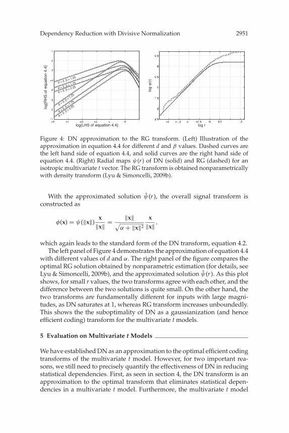
Figure 4: DN approximation to the RG transform. (Left) Illustration of theapproximation in equation 4.4 for different d and β values. Dashed curves arethe left hand side of equation 4.4, and solid curves are the right hand side ofequation 4.4. (Right) Radial maps ψ(r ) of DN (solid) and RG (dashed) for anisotropic multivariate t vector. The RG transform is obtained nonparametricallywith density transform (Lyu & Simoncelli, 2009b).

With the approximated solution ψ(r ), the overall signal transform isconstructed as

φ(x) = ψ(‖x‖)x

‖x‖ = ‖x‖√

α + ‖x‖2

x‖x‖ ,

which again leads to the standard form of the DN transform, equation 4.2.The left panel of Figure 4 demonstrates the approximation of equation 4.4

with different values of d and α. The right panel of the figure compares theoptimal RG solution obtained by nonparametric estimation (for details, seeLyu & Simoncelli, 2009b), and the approximated solution ψ(r ). As this plotshows, for small r values, the two transforms agree with each other, and thedifference between the two solutions is quite small. On the other hand, thetwo transforms are fundamentally different for inputs with large magni-tudes, as DN saturates at 1, whereas RG transform increases unboundedly.This shows the the suboptimality of DN as a gaussianization (and henceefficient coding) transform for the multivariate t models.

5 Evaluation on Multivariate t Models

We have established DN as an approximation to the optimal efficient codingtransforms of the multivariate t model. However, for two important rea-sons, we still need to precisely quantify the effectiveness of DN in reducingstatistical dependencies. First, as seen in section 4, the DN transform is anapproximation to the optimal transform that eliminates statistical depen-dencies in a multivariate t model. Furthermore, the multivariate t model

2952 S. Lyu

itself is a proxy model of natural sensory signals. Therefore, we need aquantitative evaluation of the effectiveness of the DN transform in reducingstatistical dependencies of natural sensory signals to confirm its usefulnessas an efficient coding transform.

We start with this section by applying DN to the isotropic multivariatet models, whose closed-form density allows a precise computation of thestatistical dependencies reduced by the DN transform. In the next section,we apply the DN transform to natural sensory signal data, estimate thedependency reduction, and compare the results with those predicted fromthe optimally fitted multivariate t model.

Subsequently, we employ the multi-information (MI) (Studeny &Vejnarova, 1998), also known as total variation (Watanabe, 1960) or mul-tivariate constraint (Garner, 1962), as a quantitative measure of statisticaldependencies in multivariate random variables. MI is a multivariate gen-eralization of the mutual information (Cover & Thomas, 2006) between apair of variables. For a d-dimensional random vector x with joint densityp(x), its MI is the Kullback-Leibler (KL) divergence (Cover & Thomas,2006) between the joint model and the product of marginals of all itscomponents:

I (x)=KL

(

p(x)

∥∥∥∥∥

d∏

k=1

p(xk)

)

=∫

xp(x) log

(

p(x)

/d∏

k=1

p(xk)

)

dx. (5.1)

MI is always nonnegative, and I (x) = 0 if and only if the components of x aremutually independent. An important property of MI is that for a transformof x defined as φ(x) = (φ1(x1), . . . , φd (xd ))′, where {φk(·)}d

k=1 are univariateand continuously differentiable functions, we have I (x) = I (φ(x)). This is adirect result of the change of variable procedure on the probability distri-butions of continuous random variables.

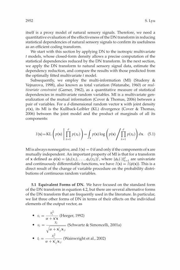
5.1 Equivalent Forms of DN. We have focused on the standard formof the DN transform in equation 4.2, but there are several alternative formsof the DN transform that are frequently used in the literature. In particular,we list three other forms of DN in terms of their effects on the individualelements of the output vector, as

� si = x2i

α + x′x(Heeger, 1992)

� vi = xi√α + x′

\i x\i

(Schwartz & Simoncelli, 2001a)

� ti = x2i

α + x′\i x\i

(Wainwright et al., 2002)


However, the outputs of these DN transforms have the same MI asthat of equation 4.2. Hence, they are all equivalent as efficient codingtransforms.

To better see this, first recall the property of the MI that it is invari-ant to any continuously differentiable element-wise transform. The threealternative DN transforms are related to the standard DN form by continu-ously differentiable transforms that map between corresponding elements.Specifically, denoting the output of the standard DN form by u, the outputof the first DN transform can be expressed as an element-wise square of uas si = u2

i . The origin of the second form of DN is a division of xi with theconditional standard deviation of xi given the remaining components in x(see section 3). In this case, we have

vi = xi√α + x′

−i x−i= xi√

α + x′x − x2i

= xi/√

α + x′x√

1 − x2i /(α + x′x)

= ui√1 − u2

i

,

which is an element-wise nonlinear transformation of u. Finally, the sameis true for the third form of the DN transform, as ti = v2

i = u2i /(1 − u2

i ).

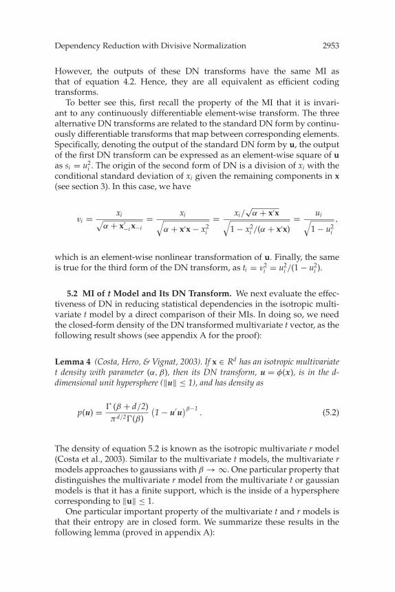
5.2 MI of t Model and Its DN Transform. We next evaluate the effec-tiveness of DN in reducing statistical dependencies in the isotropic multi-variate t model by a direct comparison of their MIs. In doing so, we needthe closed-form density of the DN transformed multivariate t vector, as thefollowing result shows (see appendix A for the proof):

Lemma 4 (Costa, Hero, & Vignat, 2003). If x ∈ Rd has an isotropic multivariatet density with parameter (α, β), then its DN transform, u = φ(x), is in the d-dimensional unit hypersphere (‖u‖ ≤ 1), and has density as

p(u) = � (β + d/2)πd/2�(β)

(1 − u′u

)β−1. (5.2)

The density of equation 5.2 is known as the isotropic multivariate r model(Costa et al., 2003). Similar to the multivariate t models, the multivariate rmodels approaches to gaussians with β → ∞. One particular property thatdistinguishes the multivariate r model from the multivariate t or gaussianmodels is that it has a finite support, which is the inside of a hyperspherecorresponding to ‖u‖ ≤ 1.

One particular important property of the multivariate t and r models isthat their entropy are in closed form. We summarize these results in thefollowing lemma (proved in appendix A):

2954 S. Lyu

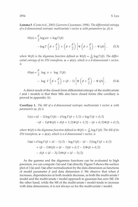
Lemma 5 (Costa et al., 2003; Guerrero-Cusumano, 1996). The differential entropyof a d-dimensional isotropic multivariate t vector x with parameters (α, β) is

H(x) = d2

log απ + log �(β)

− log �

(β + d

2

)+

(β + d

2

) [

(β + d

2

)− (β)

], (5.3)

where (β) is the digamma function defined as (β) = ddβ

log �(β). The differ-ential entropy of its DN transform, u = φ(x), which is a d-dimensional r vector,is

H(u) = d2

log π + log �(β)

− log �

(β + d

2

)+ (β − 1)

[

(β + d

2

)− (β)

]. (5.4)

A direct result of the closed-form differential entropy of the multivariatet and r models is that their MIs also have closed forms (the corollary isproved in appendix A):

Corollary 1. The MI of a d-dimensional isotropic multivariate t vector x withparameters (α, β) is

I (x) = (d − 1) log �(β) − d log �(β + 1/2) + log �(β + d/2)

−(d − 1)β(β) + d(β + 1/2)(β + 1/2) − (β + d/2)(β + d/2),

where (β) is the digamma function defined as (β) = ddβ

log �(β). The MI of itsDN transform, u = φ(x), which is a d-dimensional r vector, is

I (u) = d log �(β + (d − 1)/2) − log �(β) − (d − 1) log �(β + d/2)

+ (β − 1)(β) + (d − 1)(β + d/2 − 1)(β + d/2)

− d(β + (d − 3)/2)(β + (d − 1)/2).

As the gamma and the digamma functions can be evaluated to highprecision, we can compute I (x) and I (u) directly. Figure 5 shows the surfaceplot of I (x) and I (u) after normalization by the data dimension as functionsof model parameter β and data dimension d. We observe that when β

increases, dependencies in both models decrease, as both the multivariate tmodel and the multivariate r model approach to gaussian has zero MI. Onthe other hand, while the MI of the multivariate t model tends to increasewith data dimensions, it is not always so for the multivariate r model.


Figure 5: Surface plot of the unit MI normalized by the data dimension forthe isotropic multivariate t model (left) and the isotropic multivariate r model(right) with different β and d values.

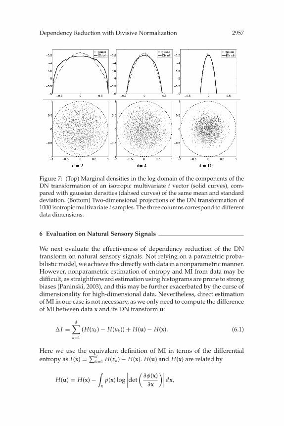
5.3 Dependency Reduction with DN. With these results, we can com-pute the change of MI per dimension of the input, �I/d = (I (x) − I (u))/d ,as a function of β and d. The left column of Figure 6 shows �I/d , and theright column shows �I/I (x), which is the MI change relative to the rawstatistical dependencies in x. For d > 4, MI are reduced after DN is appliedto the multivariate t models. The reduction increases with data dimension-ality for fixed β values (middle row, Figure 6) and decreases with increasedshape parameter β for the fixed data dimension (bottom row, Figure 6).The dependencies reduced with the DN transform are also reflected by thegaussianization effect of its outputs. Shown in the top row of Figure 7 are1D marginal densities of the DN transformed multivariate t vectors withβ = 1.1 and different dimensions. As it shows, for higher data dimension,(e.g., d = 10), the marginal distribution becomes quite close to the gaussianmodel.

However, when d ≤ 4, the changes in MI are consistently negative for allβ values, indicating that the outputs of the DN transform have increasedstatistical dependencies compared to the inputs. One intuitive explanationis that the small number of components in low-dimensional x leads to infe-rior estimations of the latent variable z, and thus a weaker gaussianizationeffect (Schwartz, Sejnowski, & Dayan, 2006). This can be further confirmedwith the marginal distributions of the DN-transformed multivariate t vec-tors of different dimensions (top row, Figure 7). The marginal distributionsfor low-dimensional inputs (e.g., d = 2) are quite different from a gaussian.

Another interpretation may be obtained by observing the two-dimensional projections of the DN-transformed multivariate t vectors ofdifferent dimensions (bottom row, Figure 7). As the plots show, for low-dimensional inputs (e.g., d = 2), a significant fraction of the 2D projectionsare around the unit circle, which is the boundary of support of the corre-sponding 2D r distribution. Samples near this boundary have strong sta-tistical dependencies (e.g., knowing one has a coordinate near ±1, we can

2956 S. Lyu

Figure 6: (Left column). Absolute change of MI normalized by the data dimen-sionality, �I/d . (Right column). Same plots for relative changes of MI, �I/I (x).The top row shows surface plots with the full range of data dimensions (d) andthe shape parameter of (β). The middle and bottom rows show slices of thecorresponding surface plots in the top row for fixed β and d, respectively.

predict that the other component has a coordinate close to 0.0), while sam-ples in the central region are closer to being gaussian distributed and lessdependent. For low-dimensional data, the increased dependencies near theboundary may counteract the reduced dependencies of the central region;hence, the net effect is an increased MI. On the other hand, for a higherdata dimension (e.g., d = 10), the majority of the projected samples are far-ther away from the unit circle, with weakened dependencies caused by theboundary constraint; hence the overall dependencies are reduced.


Figure 7: (Top) Marginal densities in the log domain of the components of theDN transformation of an isotropic multivariate t vector (solid curves), com-pared with gaussian densities (dahsed curves) of the same mean and standarddeviation. (Bottom) Two-dimensional projections of the DN transformation of1000 isotropic multivariate t samples. The three columns correspond to differentdata dimensions.

6 Evaluation on Natural Sensory Signals

We next evaluate the effectiveness of dependency reduction of the DNtransform on natural sensory signals. Not relying on a parametric proba-bilistic model, we achieve this directly with data in a nonparametric manner.However, nonparametric estimation of entropy and MI from data may bedifficult, as straightforward estimation using histograms are prone to strongbiases (Paninski, 2003), and this may be further exacerbated by the curse ofdimensionality for high-dimensional data. Nevertheless, direct estimationof MI in our case is not necessary, as we only need to compute the differenceof MI between data x and its DN transform u:

�I =d∑

k=1

(H(xk) − H(uk)) + H(u) − H(x). (6.1)

Here we use the equivalent definition of MI in terms of the differentialentropy as I (x) = ∑d

k=1 H(xk) − H(x). H(u) and H(x) are related by

H(u) = H(x) −∫

xp(x) log

∣∣∣∣det(

∂φ(x)∂x

)∣∣∣∣ dx,

2958 S. Lyu

where the Jacobian determinant of the standard form of DN transform is

det(

∂φ(x)∂x

)= α

(α + x′x)d/2+1 .

Replacing these results back to equation 6.1, we have

�I =d∑

k=1

(H(xk) − H(uk)) + log α −(

d2

+ 1) ∫

xp(x) log (α + x′x) dx.

(6.2)

The first term computes the total difference between differential entropyof corresponding components of x and u. The entropy of each componentis estimated with the nonparametric m-spacing entropy estimator (Vasicek,1976) (see appendix C). The last term in equation 6.2 is the expectation oflog (α + x′x) with regard to p(x), which can be well approximated with aver-ages over a sufficient number of samples from p(x). The only free parameteris α, which we determine by a direct search for a value that maximizes theresulting �I over a range of values. We test this nonparametric estimationof �I with samples from the isotropic multivariate t model and comparethe results with the theoretical values computed using lemma 1. Figure 8shows two cases of this comparison—one with fixed β in the model andvarying d values and the other with fixed d and varying β values. Asthese results show, the nonparametric estimations are very close to thethe theoretical ground-truth values, justifying their uses in the subsequentexperiments.

6.1 Experiments with Natural Audio and Image Data. We next per-form experiments with natural audio and image data. For audio data, weuse 10 sound clips of animal vocalization and recordings in natural environ-ments, which have a sampling frequency of 44.1 kHz and a typical lengthof 15 to 20 seconds. These sound clips are preprocessed with a bandpassgamma-tone filter of 3 kHz center frequency (Johannesma, 1972). For im-age data, we use the central 1024 × 1024 cropped regions of 20 images oflinearized intensities from the van Hateren database (van der Schaaf & vanHateren, 1996), which are taken from natural scenes such as woods andparks. As a preprocessing step, the intensities of the image data are firstsubject to a global logarithm nonlinearity, log I (x) − C0, as in Bethge (2006),where C0 is a constant so that the adjusted log intensities of an image havemean 0. The logarithm transform loosely simulates the nonlinear intensitytransforms found in the cone photoreceptors in vertebrates (McCann, 2005).The images are then convolved with an isotropic bandpass filter obtainedfrom an unoriented steerable pyramid (Simoncelli & Freeman, 1995) that


Figure 8: Comparison of theoretical prediction of MI reduction for an isotropicmultivariate t model (solid curves) with the nonparametric estimation usingequation 6.2, with random samples drawn from the multivariate t models(dashed curves). The left plot corresponds to samples drawn from fixed β = 1.10and different data dimensions, and the right plot corresponds to those drawnfrom a model of d = 10 and varying β.

Figure 9: Mean and standard deviation of the estimated shape parameter β onnatural sound data sets and natural image data sets with different dimensions.

captures an annulus of frequencies in the Fourier domain ranging from π/4to π radians per pixel, followed by a proper downsampling. We then extractadjacent samples using localized 1D temporal (for audios) or 2D spatial (forimages) windows of different sizes. These data are vectorized and whitenedto have second-order dependencies removed.

We fit isotropic multivariate t models to data using the maximum like-lihood estimation (described in appendix B). Shown in Figure 9 are themeans and standard deviations of the estimated shape parameter β of dif-ferent sizes of local windows for audio and image data, respectively (αis determined as α = 2(β − 1) for isotropic multivariate t model fitted towhitened data with identity covariance matrix). As these plots show, theestimated β values are typically close to 1, reflecting their high kurtosis.

2960 S. Lyu

Figure 10: Unit MI changes (�I/d) on natural sound data sets and naturalimage data sets with different dimensions. The solid curve corresponds to thetheoretical value obtained with lemma 1; the dashed curve is the nonparametricestimation with equation 4.2.

Furthermore, β decreases as the dimensionality increases, indicating anincreasing trend of nongaussianity.

Based on the fitted isotropic multivariate t model, we compute the MIdifference predicted by the fitted multivariate t model (see lemma 1) andcompared the results with the nonparametric estimation of MI differencein Figure 10. The solid curves correspond to theoretical predictions, anddashed curves are results from nonparametric estimations. In both cases,we report average MI difference over all sounds or images to remove biasesof individual samples.

The nonparametric estimations of MI differences after applying DN tonatural sensory data are in accordance with their predictions from the mul-tivariate t models. Both results suggest strong positive correlation of theeffectiveness of dependency reduction of DN with data dimension. Fur-thermore, as observed in the previous section, the multivariate t modelpredicts that DN increases statistical dependency for small input dimen-sions; similar observations hold for natural sensory signal data. There arealso several distinct differences between the two sets of results. First, thepredictions based on the multivariate t model tend to overestimate the MIdifference achieved by the DN transform. More important, as the data di-mension increases, the nonparametric estimations of MI difference seemto have a decreasing trend, even though multivariate t model predictionstend to keep increasing with data dimension. One important reason forsuch behaviors is the fact that the multivariate t model is still insufficient torepresent all statistical properties of natural sensory signals, even thoughit is mathematically convenient and encapsulates some important typesof statistical dependencies. A particular characteristic of natural sensorysignals is that the statistical dependencies among their bandpass-filtered


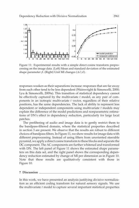
Figure 11: Experimental results with a simple direct cosine transform prepro-cessing on the image data. (Left) Mean and standard deviation of the estimatedshape parameter β. (Right) Unit MI changes (�I/d).

responses weaken as their separations increase: responses that are far awayfrom each other tend to be less dependent (Wainwright & Simoncelli, 2000;Lyu & Simoncelli, 2009a). This transition of statistical dependency cannotbe effectively captured by the multivariate t model, as any pair of com-ponents in an isotropic multivariate t vector, regardless of their relativepositions, has the same dependencies. The lack of ability to represent lessdependent or independent components using multivariate t models mayexplain the difference of the model predictions and nonparametric estima-tions of DN’s effect in dependency reduction, particularly for large localpatches.

The prefiltering of audio and image data is to gently restrict them tothe bandpass-filtered domain, where the statistical properties describedin section 3 are present. We observe that the results are robust to differentchoices of bandpass filters. In Figure 11, we show results for image data withdifferent preprocessing. Instead of using filters from unoriented steerablepyramid, we apply a direct cosine transform to these blocks and separate theDC component. The AC components are further whitened and transformedwith DN. The left panel of Figure 11 shows the estimated shape parame-ters on this data set, and the right panel shows the corresponding depen-dency reduction estimated by change of MI per dimension as in Figure 10.Note that these results are qualitatively consistent with those inFigure 10.

7 Discussion

In this work, we have presented an analysis justifying divisive normaliza-tion as an efficient coding transform for natural sensory signals. We usethe multivariate t model to capture several important statistical properties

2962 S. Lyu

of natural sensory signals in the bandpass-filtered domains. DN thenemerges as an approximation to two different optimal nonlinear transformsthat eliminate statistical dependencies in the multivariate t model. Thoughfocusing on one specific form of the DN transform, we show that severalalternative forms of DN are equivalent in terms of their effects in depen-dency reduction. In addition, we use the analytical form of the multivariatet model to provide a precise quantification of the statistical dependenciesreduced by the DN transform, which are used as a theoretical predictionof the actual performance of DN on natural sensory signal data. Moving toreal natural sensory signal data, we provide a simple method to estimatethe dependency reduction with DN nonparametrically. Our analyses con-firm DN as an effective and efficient coding transform for natural sensorysignals in bandpass-filtered domains. In the experiments, we observe a pre-viously unreported phenomenon that when the input has low dimensions,DN increases statistical dependencies for both the multivariate t modelsand natural sensory signal ensemble.

In this work, we also studied radial gaussianization analytically in thecontext of the multivariate t model and derived an explicit expression thatdirectly yields DN as an approximation to it. One distinct characteristic ofthe form of the DN transform is that the output saturates for large inputs(see the right panel of Figure 4), while the RG map is monotonically increas-ing. On one hand, this elucidates that DN cannot be the optimal efficientcoding transform for any isotropic source model. On the other hand, theDN transform seems more plausible for a biological sensory system, as theinputs and outputs to sensory neurons are always bounded. One interest-ing open question is whether DN will emerge as an optimal solution to theefficient coding objective with ecological constraints.

Finally, our analyses are based on DN of equation 4.2 and its severalequivalent forms, which are all based on the L2 norm of the input vectors.More flexible forms of the DN transform use the general Lp norms and allowthe denominator and the numerator to have different degrees. Such generalforms of the DN transform are more flexible. We envision and are workingon a similar analysis of the dependency reduction effects of such generalforms of the DN transform, using a generalized multivariate t model basedon Lp norms (Sinz & Bethge, 2009)).

Appendix A: Proof

A.1 Proof of Lemma 1. To prove the lemma, we use the basic factthat the multivariate t model is a gaussian scale mixture with an inversegamma scaling variable. Specifically, we can express the joint distributionas p(x) = ∫

z p(x|z)p(z)dz, where p(x|z) is a gaussian distribution with zeromean and covariance matrix z�, while p(z) is an inverse gamma distributionwith parameter (α, β).


The conditional mean of xi given x\i is then given by

E(xi |x\i ) =∫

xi

xi p(xi |x\i ) dxi =∫

xixi p(x) dxi

p(x\i )=

∫xi ,z

xi p(x, z) dxi dz∫

xi ,zp(x, z) dxi dz

=∫

z p(z)p(x\i |z) dz∫

xixi p(xi |x\i , z) dxi

∫z p(z)p(x\i |z) dz

.

With the property of gaussian distributions (Feller, 1968), we note thatp(xi |x\i , z) is a 1D gaussian density, whose mean and variance are�′

\i,i�−1\i,\i x\i and z(�i,i − �′

\i,i�−1\i,\i�\i,i ), respectively. Therefore, we have

E(xi |x\i ) = E(xi |x\i , z) = �′\i,i�

−1\i,\i x\i .

Next, we compute the conditional variance:

var(xi |x\i ) =∫

xi

(xi − E(xi |x\i ))2 p(xi |x\i ) dxi

=∫

z p(z)p(x\i |z) dz∫

xi(xi − E(xi |x\i , z))2 p(xi |x\i , z) dxi

∫z p(z)p(x\i |z) dz

= (�i,i − �′

\i,i�−1\i,\i�\i,i

)∫

z zp(z)p(x\i |z) dz∫

z p(z)p(x\i |z) dz.

The ratio in the last step can be further simplified if we notice that

∫z zp(z)p(x\i |z) dz∫

z p(z)p(x\i |z) dz=

∫z zpγ −1 (z;α, β)N (x\i/

√z) dz

∫z pγ −1 (z;α, β) dzN (x\i/

√z) dz

= α�(β − 1)2�(β)

∫z pγ −1 (z;α, β − 1)N (x\i/

√z) dz


√z) dz

= α

2(β − 1)

∫z pγ −1 (z;α, β − 1)N (x\i/

√z) dz


√z) dz

.

Notice that the numerator is the GSM form of a multivariate t model of thed − 1 dimension with parameter α and β − 1, while the denominator is amultivariate t model of the d − 1 dimension with parameters α and β, sothe last step can be further simplified as

α

2(β − 1)

αβ−1�(β−1+(d−1)/2)π (d−1)/2�(β−1)

(α + x′

\i�−1\i,\i x\i

)−(β−1)−(d−1)/2

αβ�(β+(d−1)/2)π (d−1)/2�(β) (α + x′

\i�−1\i,\i x\i )−β−(d−1)/2

,

2964 S. Lyu

which, after simplifying the terms, becomes E(x2i |x\i ) = 1

2β+d−3 (α +x′

\i�−1\i,\i x\i ). Collecting all terms together, we have

var(xi |x\i ) = �i,i − �′\i,i�

−1\i,\i�\i,i

2β + d − 3(α + x′

\i�−1\i,\i x\i ).

A.2 Proof of Lemma 2.

Corollary 2. The mean and mode of the inverse gamma density, pγ −1 (z;α, β) =αβ

2β�(β) z−β−1 exp(− α2z ), is α

2(β−1) and α2(β+1) , respectively. Furthermore, the mean of

1/z with regard to the inverse gamma density is 2β/α.

Proof. For the mean of the inverse gamma density, we have

∫ ∞

0zpγ −1 (z;α, β)dz =

∫ ∞

0z · αβ

2β�(β)z−β−1 exp

(− α

2z

)dz

= αβ

2β�(β)

∫ ∞

0z−β exp

(− α

2z

)dz.

Using the property of the gamma function, the last integral equals(a/2)−(β−1)�(β − 1). As �(β)/�(β − 1) = β − 1, we show that the mean isα/[2(β − 1)].

Next, the mode of the inverse gamma density corresponds to the z valuewith the maximum log density, which is given by

log pγ −1 (z;α, β) = log αβ − log 2β�(β) − (β + 1) log z − α

2z,

whose derivative with regard to z is − β+1z + α

2z2 . Setting the derivative to0 and solving for z, we obtain the mode of the inverse gamma density asα/[2(β + 1)].

Finally, the mean of 1/z in the inverse gamma density is defined as

∫ ∞

0z−1 pγ −1 (z;α, β)dz = αβ

2β�(β)

∫ ∞

0z−β−2 exp

(− α

2z

)dz.

Using the property of the gamma function, we find that the last integralequals (a/2)−(β+1)�(β + 1). Putting this result back and using the propertyof the gamma function that �(β + 1)/�(β) = β, we simplify the result to2β/α.

Now we turn to prove lemma 2. We first show that the posterior densityof z in the multivariate t model is also an inverse gamma density, as we


have

p(z|x;α, β) = p(x, z;α, β)pt(x;α, β)

=1

(2π )d/2zd/2 exp(− 1

2z x′x)

αβ

2β�(β) z−β−1 exp(− α

2z

)

αβ�(β+d/2)πd/2�(β)

1(α+x′x)β+d/2

.

Rearranging terms, we have

p(z|x;α, β) = (α + x′x)β+d/2

2β+d/2� (β + d/2)z−β−d/2−1 exp

(− 1

2z

(α + x′x

)),

which is an inverse gamma density with (α + x′x, β + d/2). The result isimmediate with corollary 2.

A.3 Proofs of Lemma 3. We first prove equation 6.4. The first-orderTaylor series approximation of function x log x for x ≥ 1 is x log x ≈ x − 1.Replacing with x = 1 + u, we have log(1 + u) ≈ 1 − 1

1+u = u1+u . Next, set u =

r2/α. We have log(α + r2) ≈ log α + r2

α+r2 , so − α2 log(α + r2) ≈ − α

2 log α −α2

r2

α+r2 , or (α + r2)−α2 ≈ α− α

2 exp(− α2

r2

α+r2 ).Next, replace the right-hand side of equation 6.3 with 6.4. Dropping

scaling factors, we now show that ψ(r ) = r√α+r2 provides a solution to the

resulting differential equation. This is achieved by replacing ψ ′(r ) = α(α+r2)3/2

on the left-hand side of equation 6.3. Merging similar terms, we have

ψ(r )d−1 exp(

−αψ2(r )2

)|ψ ′(r )|

= rd−1

(α + r2)(d−1)/2exp

(− αr2

2(α + r2)

)α

(α + r2)3/2 ,

which equates the left-hand side of equation 6.3 with the approximation ofits right-hand side with equation 6.4.

A.4 Proofs of Lemma 4. The relation between densities of transformedrandom vector gives that p(x) = p(φ(x)) det(Jφ(x)) or p(u) = p(x) 1

det(Jφ (x)) .Using the Jacobian determinant of the DN transform, we have

p(u) = αβ�(β + d/2)πd/2�(β)

(α + x′x)d/2 + 1

α(α + x′x)β + d/2 = αβ−1�(β + d/2)πd/2�(β)

1−(α + x′x)β−1 .

(A.1)

2966 S. Lyu

Next, note that

u = x√α + x′x

⇒ u′u = x′xα + x′x

⇒ ‖x‖ =√

α‖u‖√1 − u′u

.

Therefore, as x/‖x‖ = u/‖u‖, we have x =√

αu√1−‖u‖2

. Replacing this with

equation A.1, we have

p(u) = αβ−1� (β + d/2)πd/2�(β)

1(α + αu′u

1−u′u

)β−1 = � (β + d/2)πd/2�(β)

(1 − u′u)β−1.

A.5 Proof of Lemma 5. The entropy of a multivariate t and r models isin closed form (Costa et al., 2003), and we provide the derivation here forcompleteness of this work.

Evaluating H(x). We first expand H(x) based on its definition as

H(x) = d2

log π − β log α + log �(β) − log �(β + d/2)

+ (β + d/2)∫

xlog(α + x′x)pt(x;α, β) dx. (A.2)

To compute the last term in equation A.2, we use the normalizing propertyof the multivariate t model as

∫

x

(α + x′x

)−β−d/2dx = πd/2�(β)αβ� (β + d/2)

.

Taking the derivative with regard to β to both sides, we have

−∫

x

(α + x′x

)−β−d/2 log(α + x′x)dx = ∂

∂β

(πd/2�(β)

αβ� (β + d/2)

).

Multiplying −αβ� (β + d/2)/πd/2�(β) on both sides, we obtain

∫

xlog(α + x′x)pt(x;α, β) dx = − ∂

∂β

(πd/2�(β)

αβ� (β + d/2)

)αβ� (β + d/2)

πd/2�(β)

= ∂

∂βlog

αβ� (β + d/2)�(β)

= log α + (β + d/2) − (β).

Replacing the integral in the last term in equation A.2 with log α + (β +d/2) − (β), we have proved equation 5.3.


Evaluating H(u). Similar to the previous case, we first expand H(u) as

H(u) = d/2 log π + log �(β) − log �(β + d/2)

− (β − 1)∫

upτ (u;β) log

(1 − u′u

)+ du. (A.3)

We compute the integral in equation A.3 by the normalizing property of themultivariate r model. We start with

πd/2�(β)�(β + d/2)

=∫

u

(1 − u′u

)β−1+ du.

Next, taking the derivatives with regard to β and multiplying �(β+d/2)πd/2�(β) , we

have

�(β + d/2)�(β)

ddβ

�(β)�(β + d/2)

= �(β + d/2)πd/2�(β)

ddβ

∫

u

(1 − u′u

)β−1+ du

=∫

u

�(β + d/2)πd/2�(β)

(1 − u′u

)β−1+ log

(1 − u′u

)+ du

=∫

upτ (u;β) log

(1 − u′u

)+ du.

We can further simplify

�(β + d/2)�(β)

ddβ

�(β)�(β + d/2)

= ddβ

log�(β)

�(β + d/2)=(β) − (β + d/2).

Putting this result in equation A.3, we have proved equation 5.4.

A.6 Proof of Corollary 1. First, using the relation between differentialentropy and MI, we have

I (x) =d∑

k=1

H(xk) − H(x). (A.4)

To compute MI, we need to compute the joint differential entropy for mul-tivariate t and r models and the differential entropy for each component ofthe multivariate t and r vectors. The former are direct results of lemma 5,which can be obtained using the fact that each component of a multivariatet vector x has a one-dimensional t density and equation 5.3, so we have

H(xi ) = 12

log απ + log �(β) − log �(β + 1/2)

+ (β + 1/2) [ (β + 1/2) − (β)] . (A.5)

2968 S. Lyu

Furthermore, the marginal density of each element, ui, in a multivariate rvector is a one-dimensional r model with parameter β + (d − 1)/2 (Elderton,1953), as

pτ (ui ;β) = β + (d − 1)/2√π

(1 − u2i )β−1+(d−1)/2

+

Applying this to equation 5.4, the differential entropy of ui is given as(Zografos, 1999)

H(ui ) = 12

log π + log �

(β + d − 1

2

)− log �

(β + d

2

)

+(

β + d − 32

) [

(β + d

2

)−

(β + d − 1

2

)]. (A.6)

I (x) and I (u) are obtained by combining equations 5.3, 5.4, A.5, and A.6into equation A.4.

Appendix B: Maximum Likelihood Fitting of Multivariate t Model

We briefly describe the maximum likelihood fitting the multivariate t modelto using data x1, . . . , xN, which have been centered and whitened. Enforc-ing an identical covariance matrix and using the GSM equivalence of themultivariate t model, we have

I =∫

xxxT pt(x;α, β)dx

=∫

zpγ −1 (z;α, β)dz

∫

xxxTN (x/

√z)dx = α

2(β − 1)I,

the last step of which is based on fact 2. Immediately, we have α =2(β − 1), which means that we only need to estimate β. Replacing thisresult, the average log likelihood of the multivariate t model, L(β) =1N

∑Nn=1 log pt(xn; 2(β − 1), β), becomes

L(β) = β log 2(β − 1) + log �(β + d/2) − d2

log π

− log �(β) − β + d/2N

N∑

n=1

log(2(β − 1) + xTn xn).

Optimal β is the root of the nonlinear equation ddβ

L(β) = 0, which is ob-tained numerically by the Newton-Raphson procedure.


Appendix C: m-spacing Entropy Estimator

Let z1 ≤ · · · ≤ zN be the sorted set of N independent and identically dis-tributed samples of scalar random variable z. With an integer m = O(

√N),

the m-spacing entropy estimation of H(z) is defined as

H(z1, . . . , zN) = 1N

N−m∑

i=1

log(

Nm

[zi+m − zi ])

− (m) + log(m),

where (x) = ddx log �(x) is the digamma function. The m-spacing estimator

is strongly consistent—P(limm→∞,m/N→0 H(z1, . . . , zN) = H(z)

) = 1.

Acknowledgments

Thanks to Eero Simoncelli for helpful discussions and the two anonymousreferees for their critical and constructive comments. This material is basedon work supported by the National Science Foundation under CAREERAward grant no. 0953373. Any opinions, findings, and conclusions or rec-ommendations expressed in this material are my own and do not necessarilyreflect the views of the National Science Foundation.

References

Andrews, D. F., & Mallows, C. L. (1974). Scale mixtures of normal distributions.Journal of the Royal Statistical Society. Series B (Methodological), 36(1), 99–102.

Atick, J. J. (1992). Network Could information theory provide an ecological theoryof sensory processing? Network, 3, 213–251.

Atick, J. J., Li, Z., & Redlich, A. N. (1992). Understanding retinal color coding fromfirst principles. Neural Computation, 4, 559–572.

Atick, J. J., & Redlich, A. N. (1992). What does the retina know about natural scenes?Neural Computation, 4, 196–210.

Attneave, F. (1954). Some informational aspects of visual perception. Psych. Rev., 61,183–193.

Baddeley, R. (1996). Searching for filters with “interesting” output distributions: Anuninteresting direction to explore. Network, 7, 409–421.

Barlow, H. B. (1961). Possible principles underlying the transformation of sensorymessages. In W. A. Rosenblith (Ed.), Sensory Communication (pp. 217–234). Cam-bridge, MA: MIT Press.

Barlow, H. (2001). Redundancy reduction revisited. Network, 12, 241–253.Bell, A. J., & Sejnowski, T. J. (1997). The “independent components” of natural scenes

are edge filters. Vision Research, 37(23), 3327–3338.Bethge, M. (2006). Factorial coding of natural images: How effective are linear models

in removing higher-order dependencies? J. Opt. Soc. Am. A, 23(6), 1253–1268.Brady, N., & Field, D. J. (2000). Local contrast in natural images: Normalisation and

coding efficiency. Perception, 29, 1041–1055.

2970 S. Lyu

Burt, P., & Adelson, E. (1981). The Laplacian pyramid as a compact image code. IEEETransactions on Communication, 31(4), 532–540.

Carandini, M., & Heeger, D. J. (1994). Summation and division by neurons in primatevisual cortex. Science, 264, 1333–1336.

Carandini, M., Heeger, D. J., & Senn, W. (2002). A synaptic explanation of suppressionin visual cortex. Journal of Neuroscience, 22(22), 10053–10065.

Chantas, G., Galatsanos, N., Likas, A., & Saunders, M. (2008). Bayesian image restora-tion based on a product of t-distributions image prior. IEEE Transactions on ImageProcessing, 17(10), 1795–1820.

Chichilnisky, E. (2001). A simple white noise analysis of neuronal light responses.Network, 12, 199–213.

Costa, J., Hero, A., & Vignat, C. (2003). On solutions to multivariate maximumα-entropy problems. In Proceedings of Energy Minimization Methods in ComputerVision and Pattern Recognition. New York: Springer.

Cover, T., & Thomas, J. (2006). Elements of information theory (2nd ed.). Hoboken, NJ:Wiley-Interscience.

Deneve, S., Pouget, A., & Latham, P. (1999). Divisive normalization, line attractornetworks and ideal observers. In M. Kearns, S. A. Solla, & D. A. Cohn (Eds.),Advances in neural processing systems 11 (pp. 104–110). Cambridge, MA: MIT Press.

Eichhorn, J., Sinz, F., & Bethge, M. (2009). Natural image coding in V1: How muchuse is orientation selectivity? PLoS Computational Biology, 5(4), 1–16.

Elderton, W. (1953). Frequency curves and correlations. General Books LLC.Feller, W. (1968). An Introduction to probability theory and its applications. Hoboken, NJ:

Wiley.Field, D. J. (1987). Relations between the statistics of natural images and the response

properties of cortical cells. Journal of the Optical Society of America A, 4(12), 2379–2394.

Foley, J. (1994). Human luminance pattern mechanisims: Masking experiments re-quire a new model. J. of Opt. Soc. of Amer. A, 11(6), 1710–1719.

Gao, D., & Vasconcelos, N. (2009). Decision-theoretic saliency: Computational prin-ciples, biological plausibility, and implications for neurophysiology and psy-chophysics. Neural Computation, 21, 239–271.

Garner, W. R. (1962). Uncertainty and structure as psychological concepts. Hoboken, NJ:Wiley.

Guerrero-Cusumano, J.-L. (1996). A measure of total variability for the multivari-ate t distribution with applications to finance. Information Sciences, 92(1–4), 47–63.

Heeger, D. J. (1992). Normalization of cell responses in cat striate cortex. Visual NeuralScience, 9, 181–198.

Holt, G. R., & Koch, C. (1997). Shunting inhibition does not have a divisive effect onfiring rates. Neural Computation, 9, 1001–1013.

Jarrett, K., Kavukcuoglu, K., Ranzato, M., & LeCun, Y. (2009). What is the best multi-stage architecture for object recognition? In Proceedings of the 12th IEEE Conferenceon Computer Vision. Piscataway, NJ: IEEE.

Johannesma, P. (1972). The pre-response stimulus ensemble of neurons in thecochlear nucleus. In Symposium on Hearing Theory (pp. 58–69). Eindhoven,Holland: IPO.


Kac, M. (1939). On a characterization of the normal distribution. American Journal ofMathematics, 61(3), 726–728.

Kotz, S., & Nadarajah, S. (2004). Multivariate t distributions and their applications.Cambridge: Cambridge University Press.

Laparra, V., Munoz-Mari, J., & Malo, J. (2010). Divisive normalization image qualitymetric revisited. Journal of the Optical Society of America A, 27(4), 852–864.

Lee, J., & Maunsell, J. H. R. (2009). A normalization model of attentional modulationof single unit responses. PLoS One, 4(2), 1–13.

Lewicki, M. S. (2002). Efficient coding of natural sounds. Nature Neuroscience, 5(4),356–363.

Li, Q., & Wang, Z. (2008). General-purpose reduced-reference image quality assess-ment based on perceptually and statistically motivated image representation. InIEEE 15th Int’l. Conf. on Image Proc. (Vol. 15, pp. 1192–1195). Piscataway, NJ: IEEE.

Lyu, S. (2009). An implicit Markov random field model for natural images in multi-scale oriented representations. In Proceedings of the IEEE Conference on ComputerVision and Pattern Recognition. Piscataway, NJ: IEEE.

Lyu, S. (2010). Divisive normalization: Justification and effectiveness as effi-cient coding transform. In D. Koller, D. Schuurmans, Y. Bengio, & L. Bottou(Eds.). Advances in neural information processing systems, 21. Cambridge, MA:MIT Press.

Lyu, S., & Simoncelli, E. P. (2008). Nonlinear image representation using divisivenormalization. In Proceedings of the IEEE Conference on Computer Vision and PatternRecognition. Piscataway, NJ: IEEE.

Lyu, S., & Simoncelli, E. P. (2009a). Modeling multiscale subbands of photographicimages with fields of gaussian scale mixtures. In IEEE Trans. Patt. Analysis andMachine Intelligence, 31(4), 693–706.

Lyu, S., & Simoncelli, E. P. (2009b). Nonlinear extraction of “independent compo-nents” of natural images using radial gaussianization. Neural Computation, 18(6),1–35.

Malo, J., Epifanio, I., Navarro, R., & Simoncelli, E. P. (2006). Non-linear image rep-resentation for efficient perceptual coding. IEEE Transactions on Image Processing,15(1), 68–80.

Malo, J., & Laparra, V. (2010). Psychophysically tuned divisive normalization factor-izes the PDF of natural images. Neural Computation, 22, 3179–3206.

Mante, V., Bonin, V., & Carandini, M. (2008). Functional mechanisms shaping lateralgeniculate responses to artificial and natural stimuli. Neuron, 58, 625–638.

McCann, J. (2005). Rendering high-dynamic range images: Algorithms that mimichuman vision. In Proc. AMOS Technical Conf. (pp. 19–28) Maui: Maui EconomicDevelopment Board Publications.

Nash, D., & Klamkin, M. S. (1976). A spherical characterization of the normal distri-bution. Journal of Multi-Variate Analysis, 55, 56–158.

Olsen, S. R., Bhandawat, V., & Wilson, R. I. (2010). Divisive normalization in olfactorypopulation codes. Neuron, 66(2), 287–299.

Olshausen, B. A., & Field, D. J. (1996). Emergence of simple-cell receptive fieldproperties by learning a sparse code for natural images. Nature, 381, 607–609.

Paninski, L. (2003). Estimation of entropy and mutual information. Neural Comput.,15(6), 1191–1253.

2972 S. Lyu

Pillow, J. W., & Simoncelli, E. P. (2006). Dimensionality reduction in neural models:An information theoretic generalization of spike-triggered average and covari-ance analysis. Journal of Vision, 6, 414–428.

Reynolds, J. H., & Heeger, D. J. (2009). The normalization model of attention. Neuron,61, 168–185.

Ringach, D. L. (2010). Population coding under normalization. Vision Research, 50,2223–2232.

Roth, S., & Black, M. (2005). Fields of experts: A framework for learning image priors.In Proceedings of the IEEE International Conference on Computer Vision and PatternRecognition (Vol. 2, pp. 860–867). Piscataway, NJ: IEEE.

Ruderman, D. L., Cronin, T. W., & Chiao, C.-C. (1998). Statistics of cone responsesto natural images: Implications for visual coding. Journal of the Optical Society ofAmerica A, 15(8), 2036–2045.

Rust, N. C., Schwartz, O., Movshon, J. A., & Simoncelli, E. P. (2005). Spatiotemporalelements of macaque V1 receptive fields. Neuron, 46(6), 945–956.

Schwartz, O., Sejnowski, T. J., & Dayan, P. (2005). Assignment of multiplicativemixtures in natural images. In L. K. Saul, Y. Weiss, & L. Bottou (Eds.), Advancesin neural information processing systems, 17. Cambridge, MA: MIT Press.

Schwartz, O., Sejnowski, T. J., & Dayan, P. (2006). Soft mixer assignment in a hierar-chical model of natural scene statistics. Neural Computation, 18, 2680–2718.

Schwartz, O., & Simoncelli, E. P. (2001a). Natural signal statistics and sensory gaincontrol. Nature Neuroscience, 4(8), 819–825.

Schwartz, O., & Simoncelli, E. P. (2001b). Natural sound statistics and divisive nor-malization in the auditory system. In T. K. Leen, T. G. Dietterich, & V. Tresp(Eds.), Advances in neural information processing systems, 13 (pp, 166–172). Cam-bridge, MA: MIT Press.

Shapley, R., & Enroth-Cugell, C. (1984). Visual adaptation and retinal gain control.Progress in Retinal Research, 3, 263–346.

Simoncelli, E. P., & Buccigrossi, R. W. (1997). Embedded wavelet image compressionbased on a joint probability model. In Proc 4th IEEE Int’l Conf on Image Proc. (Vol. I,pp. 640–643). Piscataway, NJ: IEEE.

Simoncelli, E. P., & Freeman, W. T. (1995). The steerable pyramid: A flexible ar-chitecture for multi-scale derivative computation. In Proceedings of the IEEE In-ternational Conference on Image Processing (Vol. 3, pp. 444–447). Piscataway, NJ:IEEE.

Simoncelli, E. P., & Heeger, D. J. (1998). A model of neuronal responses in visual areaMT. Vision Research, 38(5), 743–761.

Sinz, F. H., & Bethge, M. (2009). The conjoint effect of divisive normalization andorientation selectivity on redundancy reduction. In D. Koller, D. Schuurmans, Y.Bengio, & L. Bottou (Eds.), Advances in neural information processing systems, 21.Cambridge, MA: MIT Press.

Solomon, S., Lee, B., & Sun, H. (2006). Suppressive surrounds and contrast gain inmagnocellular pathway retinal gangalion cells of macaque. Journal of Neuroscience,26(34), 8715–8726.

Studeny, M., & Vejnarova, J. (1998). The multi-information function as a tool formeasuring stochastic dependence. In M. I. Jordan (Ed.), Learning in graphicalmodels (pp. 261–297). Dordrecht: Kluwer.


Valerio, R., & Navarro, R. (2003a). Input-output statistical independence in divisivenormalization models of V1 neurons. Network, 14(4), 733–745.

Valerio, R., & Navarro, R. (2003b). Optimal coding through divisive normalizationmodels of V1 neurons. Network, 14(3), 579–593.

van der Schaaf, A., & van Hateren, J. H. (1996). Modelling the power spectra ofnatural images: Statistics and information. Vision Research, 28(17), 2759–2770.

Vasicek, O. (1976). A test for normality based on sample entropy. Journal of the RoyalStatistical Society, Series B, 38(1), 54–59.

Wainwright, M. J., Schwartz, O., & Simoncelli, E. P. (2002). Natural image statisticsand divisive normalization: Modeling nonlinearity and adaptation in corticalneurons. In R.P.N. Rao, B. A. Olshausen, & M. S. Lewicki (Eds.), Probabilisticmodels of the brain: Perception and neural function (pp. 203–222). Cambridge, MA:MIT Press.

Wainwright, M. J., & Simoncelli, E. P. (2000). Scale mixtures of Gaussians and thestatistics of natural images. In S. A., Solla, T. K. Leen, & K.-R. Muller (Eds.),Advances in neural information processing systems, 12 (pp. 855–861). Cambridge,MA: MIT Press.

Watanabe, S. (1960). Information theoretical analysis of multivariate correlation. IBMJournal of Research and Development, 4, 66–82.

Watson, A., & Solomon, J. (1997). A model of visual contrast gain control and patternmasking. J. Opt. Soc. Amer. A, 14, 2379–2391.

Wegmann, B., & Zetzsche, C. (1990). Statistical dependence between orientation filteroutputs used in an human vision based image code. In Proc. Visual Comm. andImage Processing (Vol. 1360, pp. 909–922). Bellingham, WA: SPIE.

Welling, M., Hinton, G. E., & Osindero, S. (2002). Learning sparse topographic rep-resentations with products of Student-t distributions. In S. Becker, S. Thrun, &K. Obermayer (Eds.), Advances in neural information processing systems (pp. 1111–1117). Cambridge, MA: MIT Press.

Zellner, A. (1971). An introduction to bayesian inference in econometrics. Hoboken, NJ:Wiley-Interscience.

Zetzsche, C., & Barth, E. (1990). Fundamental limits of linear filters in the visualprocessing of two-dimensional signals. Vision Research, 30, 1111–1117.

Zetzsche, C., & Krieger, G. (1999). The atoms of vision: Cartesian or polar? Journal ofthe Optical Society of America, A, 16, 1554–1565.

Zoccolan, D., Cox, D., & DiCarlo, J. (2005). Multiple object response normalizationin monkey inferotemporal cortex. Journal of Neuroscience, 25(36), 8150–8164.

Zografos, K. (1999). On maximum entropy characterization of Pearson’s type II andVII multivariate distributions. Journal of Multivariate Analysis, 71, 67–75.

Received September 25, 2010; accepted April 26, 2011.

Date post:	14-Mar-2020
Category:	Documents
Upload:	others
View:	16 times
Download:	0 times

Dependency Reduction with Divisive Normalization ...lsw/papers/nc11.pdfDependency Reduction with...

Documents