DERIVATION AND OBSERVABILITY OF UPPER ATMOSPHERIC …

DERIVATION AND OBSERVABILITY OF UPPER ATMOSPHERIC DENSITY

VARIATIONS UTILIZING PRECISION ORBIT EPHEMERIDES

BY

Travis Francis Lechtenberg

Submitted to the graduate degree program in Aerospace Engineering and the Graduate

Faculty of the University of Kansas in partial fulfillment of the requirements for the degree of

Master’s of Science.

Committee members

Chairperson: Dr. Craig McLaughlin

Dr. Saeed Farokhi

Dr. Shahriar Keshmiri

Date defended:

ii

The Thesis Committee for Travis Lechtenberg certifies that this is the approved Version of

the following thesis:

DERIVATION AND OBSERVABILITY OF UPPER ATMOSPHERIC DENSITY

VARIATIONS UTILIZING PRECISION ORBIT EPHEMERIDES

Committee:

Chairperson: Dr. Craig McLaughlin

Dr. Saeed Farokhi

Dr. Shahriar Keshmiri

Date approved:

iii

ABSTRACT

Several models of atmospheric density exist in today’s world, yet most

possess significant errors when compared to data determined from actual satellite

measurements. This research utilizes precision orbit ephemerides (POE) in an

optimal orbit determination scheme to generate corrections to existing density models

to better characterize observations of satellites in low earth orbit (LEO). These

corrections are compared against accelerometer derived densities that are available

for a few select satellites, notably, the CHAMP and GRACE satellites. These

corrections are analyzed by determining the cross correlation coefficients and root-

mean-squared values of the estimated corrected densities as compared to the

accelerometer derived densities for these satellites. The POE derived densities

showed marked improvement using these methods of comparison over the existing

empirical density models for all examined time periods and solar and geomagnetic

activity levels. The cross correlation values for the POE derived densities also

consistently out-performed the High Accuracy Satellite Drag Model (HASDM).

This research examines the ability of POE derived densities to characterize

short term variations in atmospheric density that occur on short time scales. The

specific phenomena examined were travelling atmospheric disturbances (TAD) and

geomagnetic cusps, which had temporal spans of less than half the period of the

satellite’s orbit, more specifically spans of between four and ten minutes, and less

than three minutes respectively. Density variations of shorter duration are more

iv

difficult to observe even in accelerometer data due to diurnal variations that arise

from cyclical increases due to the satellite passing from the darkened side of the earth

to the lit side. This research also examines the effects of a veritcally propagating

atmospheric densities by looking at periods of time during which both the GRACE

and CHAMP satellites have coplanar orbits, during which perturbations can be

examined for their capability to extend vertically through the atmosphere, as well as

their observability in POE derived densities. Additionally, this research extends the

application of optimal orbit determination techniques to an additional satellite, the

TerraSAR-X, which lacks an accelerometer.

For LEO, one of the greatest uncertainties in orbit determination is drag,

which is largely influenced by atmospheric density. There are many factors which

affect the variability of atmospheric densities, and some of these factors are well

modeled, such as atmospheric heating and to some degree, the solar and geomagnetic

activity levels, though some variations are not modeled at all.

The orbit determination scheme parameters found to perform best for most

cases were a baseline model of one of the three Jacchia based baseline models, a

density correlation half-life of 18 or 180 minutes, and a ballistic coefficient

correlation half life of 1.8 minutes. All three Jacchia based models performed very

similarly, with the CIRA-1972 model edging out the other two overall. The density

correlation half-life’s optimal value was usually 180 minutes, though for specific

levels of geomagnetic activity, a half-life of 18 minutes was preferable.

v

During the coplanar periods for both the GRACE and CHAMP satellites, both

satellites showed minor density increases that occur on the unlit side of the earth near

the equator. These increases were mostly unseen in the precision orbit ephemeris

(POE) derived densities, though the POE derived densities did show a slight response

to these perturbations. The secondary density increases were seen in both GRACE

and CHAMP accelerometer data, and likely existed both above and below the orbits

of these two satellites.

The TerraSAR-X densities found for the time period examined in this study

using POE data showed deviations from empirical density models of up to 10% for

peak atmospheric density values. The CHAMP and GRACE POE derived densities

showed a greater relative deviation from the empirical density models during peak

density periods, and the deviations for the CHAMP and GRACE satellites’

empirically predicted densities much better approximated the density values found

using the accelerometers aboard both satellites. As the TerraSAR-X satellite lacks its

own accelerometer, the POE derived densities are assumed to be a more accurate

representation of the atmospheric densities.

vi

ACKNOWLEDGEMENTS

I would like to thank Dr. Craig McLaughlin for the opportunity to perform

this research, as well as his guidance during my time in the graduate program at the

University of Kansas. His patience during the accumulation of this research is much

appreciated. I would also like to thank Doctors Keshmiri and Farokhi for their

participation on my thesis committee.

This research was made possible with the help of many different parties.

Funding for this work was provided the National Science Foundation award

#0832900 with some additional support provided by the Kansas Space Grant

Consortium. David Vallado’s help and expertise in working with data conversion

scripts and with the Orbit Determination Tool Kit (ODTK) was invaluable. Aid with

ODTK scripting was provided by Jens Ramrath at Analytical Graphics, Inc. (AGI).

Andrew Hiatt’s earlier work formed the basis for the expanded dates for which cross

correlation and root-mean squared values were found. Acclerometer derived

densities were provided by Sean Bruinsma of the Centre National d’Études Spatiales

(CNES) and density values for the High Accuracy Satellite Drag Model (HASDM)

were provided by Bruce Bowman of the U.S. Space Command.

vii

TABLE OF CONTENTS

ABSTRACT ..................................................................................................... iii

ACKNOWLEDGEMENTS ............................................................................ vi

TABLE OF CONTENTS ............................................................................... vii

NOMENCLATURE ........................................................................................ xi

LIST OF FIGURES ...................................................................................... xvii

LIST OF TABLES ......................................................................................... xix

1 INTRODUCTION ..................................................................................... 1

1.1 Objective ........................................................................................................ 1

1.2 Motivation ..................................................................................................... 1

1.3 Satellite Drag ................................................................................................. 4

1.4 Neutral Atmosphere ................................................................................... 10 1.4.1 Neutral Atmosphere Structure ...................................................................................10 1.4.2 Variations Affecting Static Atmospheric Models ......................................................11 1.4.3 Time-Varying Effects on the Thermospheric and Exospheric Density .....................12

1.5 Atmospheric Density Models ..................................................................... 16 1.5.1 Solar and Geomagnetic Indices .................................................................................17 1.5.2 Jacchia 1971 Atmospheric Model ..............................................................................19 1.5.3 Jacchia-Roberts Atmospheric Model .........................................................................20 1.5.4 CIRA 1972 Atmospheric Model ................................................................................21 1.5.5 MSISE 1990 Atmospheric Model ..............................................................................21 1.5.6 NRLMSISE 2000 Atmospheric Model ......................................................................21 1.5.7 Jacchia-Bowman Atmospheric Models .....................................................................22 1.5.8 Russian GOST Model ................................................................................................25

1.6 Previous Research on Atmospheric Density Model Corrections ............ 25 1.6.1 Dynamic Calibration of the Atmosphere ...................................................................26 1.6.2 Accelerometers ..........................................................................................................31 1.6.3 Additional Approaches ..............................................................................................36

1.7 Current Research on Atmospheric Density Model Corrections ............. 37

viii

1.8 Gauss-Markov Process ............................................................................... 39

1.9 Estimating Density and Ballistic Coefficient Separately ......................... 39

1.10 Travelling Atmospheric Disturbances (TAD) .......................................... 40

1.11 Geomagnetic Cusp Features ...................................................................... 41

1.12 Examined Satellites ..................................................................................... 42 1.12.1 CHAMP .....................................................................................................................42 1.12.2 GRACE ......................................................................................................................43 1.12.3 TerraSAR-X ...............................................................................................................44

2 Methodology ............................................................................................ 45

2.1 Precision Orbit Ephemerides ..................................................................... 45

2.2 Optimal Orbit Determination .................................................................... 46

2.3 Gauss-Markov Process Half-Lives ............................................................ 49

2.4 Filter-Smoother Description ...................................................................... 50

2.5 McReynolds’ Filter-Smoother Consistency Test ...................................... 51

2.6 Using Orbit Determination to Estimate Atmospheric Density ............... 52 2.6.1 Varying Baseline Density Model ...............................................................................54 2.6.2 Varying Density and Ballistic Coefficient Correlated Half-Lives .............................54 2.6.3 Solar and Geomagnetic Activity Level Bins ..............................................................60

2.7 Validation of the Estimated Atmospheric Density ................................... 60

2.8 Cross Correlation ........................................................................................ 61

2.9 Root Mean Squared Values ....................................................................... 62

2.10 Travelling Atmospheric Disturbances (TAD) .......................................... 62

2.11 Geomagnetic Cusp Features ...................................................................... 63

2.12 Coplanar Cases ........................................................................................... 63

2.13 Extension of Orbit Determination Techniques to TerraSAR-X ............. 64

3 EFFECTS OF VARYING SELECT ORBIT DETERMINATION

PARAMETERS ...................................................................................... 65

ix

3.1 Overall Analysis of Cross-Correlation and Root-Mean-Squared Values

for CHAMP ................................................................................................. 66

3.2 Analysis of Cross-Correlation and Root-Mean-Squared Values for

CHAMP for Varying Degrees of Geomagnetic Activity.......................... 68 3.2.1 Quiet Geomagnetic Activity Bin ...............................................................................69 3.2.2 Moderate Geomagnetic Activity Bin .........................................................................71 3.2.3 Active Geomagnetic Activity Bin ..............................................................................73 3.2.4 Summary of the Geomagnetic Activity Bins .............................................................75 3.2.5 Low Solar Activity Bin ..............................................................................................76 3.2.6 Moderate Solar Activity Bin ......................................................................................78 3.2.7 Elevated Solar Activity Bin .......................................................................................80 3.2.8 High Solar Activity Bin .............................................................................................82 3.2.9 Summary of the Solar Activity Bins ..........................................................................84

4 OBSERVABILITY OF TRAVELLING ATMOSPHERIC

DISTURBANCES IN PRECISION ORBIT EPHEMERIS DERIVED

DENSITIES ............................................................................................ 85

4.1 Cross Correlation and Root-Mean-Squared Values for April 19, 2002 . 86

4.2 Density Values for Nocturnal Passes on April 19, 2002........................... 89

4.3 Density Values for Nocturnal Passes on May 23, 2002 ............................ 94

4.4 Summary ..................................................................................................... 98

5 OBSERVABILITY OF DENSITY INCREASES LOCALIZED

AROUND THE NORTH GEOMAGNETIC POLE ........................... 99

5.1 Geomagnetic Pole Passes from April 19, 2002 ....................................... 100

5.2 Geomagnetic Pole Pass from March 21, 2003 ........................................ 102

5.3 Geomagnetic Pole Pass from February 19, 2002 .................................... 103

5.4 Summary ................................................................................................... 104

6 EXAMINATION OF COPLANAR PERIODS OF CHAMP AND

GRACE SATELLITES ....................................................................... 105

6.1 CC and RMS Values for the Coplanar Period near April 3, 2005 ....... 107

6.2 Density Values for the CHAMP and GRACE Coplanar Time Period 111

x

7 EXTENSION OF POE DENSITY DERIVATION TECHNIQUES TO

THE TERRASAR-X SATELLITE .................................................... 115

7.1 CC and RMS Values for CHAMP and GRACE for September 21-30,

2007 ............................................................................................................ 116

7.2 Density Values for September 26-27, 2007 ............................................. 119

7.3 Density Values for September 29-30, 2007 ............................................. 121

8 SUMMARY, CONCLUSIONS, AND FUTURE WORK .................. 123

8.1 Summary ................................................................................................... 123

8.2 Conclusions ................................................................................................ 127

8.3 Future Work .............................................................................................. 132 8.3.1 Considering Gravity Recovery and Climate Experiment (GRACE) Accelerometer

Derived Density Data ..............................................................................................132 8.3.2 A More Detailed Examination of the Density and Ballistic Coefficient Correlated

Half-Lives ................................................................................................................132 8.3.3 Using the Jacchia-Bowman 2008 Atmospheric Model as a Baseline Model ...........133 8.3.4 Additional Satellites with Precision Orbit Ephemerides ..........................................133

REFERENCES ............................................................................................. 135

xi

NOMENCLATURE

Symbol Definition Units

av

acceleration vector due to atmospheric drag m/s2

ap geomagnetic 3-hourly planetary equivalent amplitude

index

gamma, Tesla,

or kg s m-1

A satellite cross-sectional area m2

Ap geomagnetic daily planetary amplitude index gamma, Tesla,

or kg s m-1

B B estimated ballistic coefficient correction ~

BC ballistic coefficient m2/kg

Dc satellite drag coefficient ~

d cross correlation delay

F10.7 daily solar radio flux measured at 10.7 cm wavelength SFU

10.7F F10.7 running 81-day centered smoothed data set SFU

SF Jacchia-Bowman 2008 new solar index SFU

go gravitational acceleration m/s2

h altitude change m

i cross correlation series index

j user defined Gauss-Markov correlated half-life time

series index

k Gauss-Markov sequence index

Kp geomagnetic planetary index ~

M10.7 solar proxy for far ultra-violet radiation SFU

xii

10.7M M10.7 running 81-day centered smoothed data set SFU

m satellite mass kg

mx mean of series x

my mean of series y

M mean molecular mass amu

N number of elements

p atmospheric pressure change N/m2

po absolute pressure N/m2

P̂ filter covariance matrix

P% smoother covariance matrix

P differenced covariance matrix

r cross correlation coefficient

rv

satellite position vector m

R universal gas constant J K-1

mol-1

Rv

McReynold’s consistency test ratio

S10.7 solar extreme ultra-violet radiation at 26-34 nm

wavelength SFU

10.7S S10.7 running 81-day centered smoothed data set SFU

t time S

T temperature K

relv satellite velocity magnitude relative to Earth’s

atmosphere m/s

relvv

satellite velocity vector relative to Earth’s atmosphere m/s

xiii

w t Gaussian white random variable

x x component of satellite position vector m

x Gauss-Markov process dynamic scalar random variable

x cross correlation series

X state error

X̂ optimal state error estimate

X satellite state vector

X difference state vector

filterXv

filter state estimate

smootherXv

smoother state estimate

y measurement residual

y y component of satellite position vector m

y cross correlation series

Y10 mixed solar index SFU

z z component of satellite position vector m

xiv

Greek Letters Definition Units

Gauss-Markov process variable

estimated atmospheric density correction ~

atmospheric density kg/m3

v denominator for McReynold’s consistency test ratio

2

w variance of Gaussian white random variable

user defined correlated half-life

Earth Earth’s angular velocity magnitude rad/s

Earth

v Earth’s angular velocity vector rad/s

transition function

Abbreviations Definition

CC Cross Correlation

CHAMP Challenging Minisatellite Payload

CIRA COSPAR International Reference Atmosphere

COSPAR Committee on Space Research

CNES Centre National d’Études Spatiales

DCA Dynamic Calibration of the Atmosphere

DORIS Doppler Orbitography by Radiopositioning Integrated on Satellite

xv

Dst Disturbance Storm Time index

DTM Drag Temperature Model

ESA European Space Agency

EUV Extreme Ultra-Violet

GEOSAT Geodetic Satellite

GFO GEOSAT Follow-On

GOES Geostationary Operational Environmental Satellites

GPS Global Positioning System

GRACE Gravity Recovery And Climate Experiment

GSFC Goddard Space Flight Center

HASDM High Accuracy Satellite Drag Model

ICESat Ice, Cloud, and Land Elevation Satellite

MSISE Mass Spectrometer Incoherent Scatter Extending from ground to space

MUV Middle Ultra-Violet

NASA National Aeronautics and Space Administration

NOAA National Oceanic and Atmospheric Administration

NRLMSISE Naval Research Laboratory Mass Spectrometer Incoherent Scatter

Extending from ground to space

ODTK Orbit Determination Tool Kit

POE Precision Orbit Ephemerides

PSO Precision Science Orbit

RMS Root-Mean-Squared Value

xvi

RSO Rapid Science Orbit

SBUV Solar Backscatter Ultraviolet

SEE Solar Extreme-ultraviolet Experiment

SEM Solar Extreme-ultraviolet Monitor

SETA Satellite Electrostatic Triaxial Accelerometer

SFU Solar Flux Units

SLR Satellite Laser Ranging

SOHO Solar and Heliospheric Observatory

SOLSTICE Solar/Stellar Irradiance Comparison Experiment

SORCE Solar Radiation and Climate Experiment

STAR Spatial Triaxial Accelerometer for Research

TAD Traveling Atmospheric Disturbance

TIMED Thermosphere Ionosphere Mesosphere Energetics and Dynamics

TLE Two Line Element

UARS Upper Atmosphere Research Satellite

XRS X-Ray Spectrometer

xvii

LIST OF FIGURES

Figure 1.1: Artist Rendering of the CHAMP Satellite in Orbit .............................................. 42

Figure 1.2: Artist Rendering of the GRACE Satellites in Orbit ............................................. 43

Figure 1.3: Artist Rendering of the TerraSAR-X Satellite in Orbit ........................................ 44

Figure 4.1: Nocturnal CHAMP Satellite Densities on April 19, 2002, Orbit 7 ...................... 90



Figure 4.4: Nocturnal CHAMP Satellite Densities on April 19, 2002, Orbit 10 .................... 93

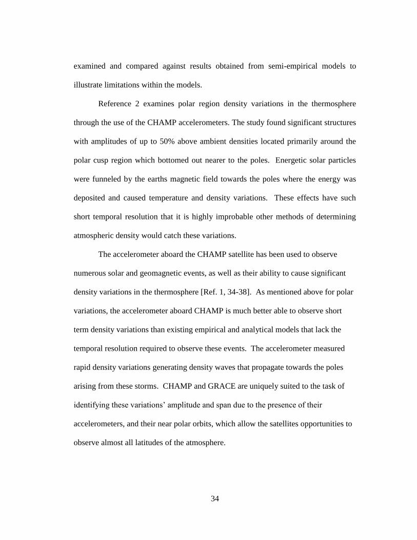
Figure 4.5: Nocturnal CHAMP Satellite Densities on May 23, 2002, Orbit 9 ....................... 95

Figure 4.6: Nocturnal CHAMP Satellite Densities on May 23, 2002, Orbit 10 ..................... 96

Figure 4.7: Nocturnal CHAMP Satellite Densities on May 23, 2002, Orbit 11 ..................... 97

Figure 5.1: CHAMP Geomagnetic Pole Pass at Approximately 22:30 UTC April 19, 2002 100

Figure 5.2: CHAMP Geomagnetic Pole Pass at Approximately 16:24 UTC April 19, 2002 101

Figure 5.3: CHAMP Geomagnetic Pole Pass at Approximately 10:14 UTC March 21, 2002

............................................................................................................................ 102

Figure 5.4: CHAMP Geomagnetic Pole Pass at Approximately 7:50 UTC February 19, 2002

............................................................................................................................ 103

Figure 6.1: CHAMP and GRACE Satellite Orbits during Coplanar Periods ....................... 106

Figure 6.2: Densities Measured and Estimated for the CHAMP and GRACE Satellites on

April 3, 2005 ....................................................................................................... 111

Figure 6.3: Densities Measured and Estimated for the CHAMP and GRACE Satellites on

April 5, 2005 ....................................................................................................... 113

Figure 7.1: Estimated and Measured Densities for CHAMP, GRACE, and TerraSAR-X,

September 26-27, 2007 ....................................................................................... 119

xviii

Figure 7.2: Estimated and Measured Densities for CHAMP, GRACE, and TerraSAR-X,

September 29-30, 2007 ....................................................................................... 121

xix

LIST OF TABLES

Table 1.1: Defined Solar and Geomagnetic Activity Bins ...................................................... 19

Table 1.2: Solar and Geomagnetic Activity Distribution........................................................ 19

Table 2.1: Dates of Available CHAMP Data and Corresponding Geomagnetic and Solar

Activity for 2001 .................................................................................................. 55


Activity for 2002 .................................................................................................. 56


Activity for 2003 .................................................................................................. 57


Activity for 2004 .................................................................................................. 58


Activity for 2005 .................................................................................................. 59


Activity for 2006 and 2007 ................................................................................... 60

Table 3.1: Zero Delay Cross Correlation Coefficients Time Averaged Across All Solutions.66

Table 3.2: Zero Delay Root-Mean-Squared Values Time Averaged Across All Solutions. .. 66

Table 3.3: Zero Delay Cross Correlation Coefficients Time Averaged for Quiet Geomagnetic

Periods. ................................................................................................................. 69

Table 3.4: Zero Delay Root-Mean-Squared Values Time averaged for Quiet Geomagnetic

Periods. ................................................................................................................. 69

Table 3.5: Zero Delay Cross Correlation Coefficients Time Averaged for Moderate

Geomagnetic Periods. ........................................................................................... 71

xx

Table 3.6: Zero Delay Root-Mean-Squared Values Time averaged for Moderate Geomagnetic

Periods. ................................................................................................................. 71

Table 3.7: Zero Delay Cross Correlation Coefficients Time Averaged for Active

Geomagnetic Periods. ........................................................................................... 73

Table 3.8: Zero Delay Root-Mean-Squared Values Time averaged for Active Geomagnetic

Periods. ................................................................................................................. 73

Table 3.9: Zero Delay Cross Correlation Coefficients Time Averaged for Low Solar Activity

Periods. ................................................................................................................. 76

Table 3.10: Zero Delay Root-Mean-Squared Values Time averaged for Low Solar Activity

Periods. ................................................................................................................. 76

Table 3.11: Zero Delay Cross Correlation Coefficients Time Averaged for Moderate Solar

Activity Periods. ................................................................................................... 78

Table 3.12: Zero Delay Root-Mean-Squared Values Time averaged for Moderate Solar


Table 3.13: Zero Delay Cross Correlation Coefficients Time Averaged for Elevated Solar


Table 3.14: Zero Delay Root-Mean-Squared Values Time averaged for Elevated Solar


Table 3.15: Zero Delay Cross Correlation Coefficients Time Averaged for High Solar


Table 3.16: Zero Delay Root-Mean-Squared Values Time averaged for High Solar Activity

Periods. ................................................................................................................. 82

Table 4.1: Cross Correlation Coefficients for All of April 19, 2002. ..................................... 86

Table 4.2: Root-Mean-Squared Values for All of April 19, 2002. ......................................... 86

xxi

Table 4.3: Cross Correlation Coefficients for Limited Nocturnal Periods of April 19, 2002. 88

Table 4.4: Root-Mean-Squared Values for Limited Nocturnal Periods of April 19, 2002. .... 88

Table 6.1: Cross Correlation Coefficients for CHAMP near April 3, 2005.......................... 107

Table 6.2: Root-Mean-Squared Values for CHAMP near April 3, 2005. ............................. 107

Table 6.3: Cross Correlation Coefficients for GRACE near April 3, 2005. ......................... 109

Table 6.4: Root-Mean-Squared Values for GRACE near April 3, 2005. ............................. 109

Table 7.1: Cross Correlation Coefficients for CHAMP for September 21-30, 2007. ........... 116

Table 7.2: Root-Mean-Squared Values for CHAMP for September 21-30, 2007. ............... 116

Table 7.3: Cross Correlation Coefficients for GRACE for September 21-30, 2007. ........... 117

Table 7.4: Root-Mean-Squared Values for GRACE for September 21-30, 2007. ................ 117

Table 8.1: Defined Solar and Geomagnetic Activity Bins .................................................... 124

Table 8.2: Optimal CC Values for CHAMP at Varying Solar and Geomagnetic Activity

Levels.................................................................................................................. 127

Table 8.3: Optimal RMS Values for CHAMP at Varying Solar and Geomagnetic Activity

Levels.................................................................................................................. 128

1

1 INTRODUCTION

1.1 Objective

The goal of this research is to utilize precision orbit ephemerides to generate

corrections to existing density models. These corrections yield more accurate density

estimates which lead to better drag estimates, improved orbit determination and

prediction, as well as an enhanced understanding of density variations in the

thermosphere and exosphere. This research primarily focuses on short term

variations such as those arising from traveling atmospheric disturbances, geomagnetic

cusps, and tides. This research will examine the ability of densities generated by

precision orbit ephemerides to characterize these short term density variations. This

examination will give a better idea of what temporal resolution can be obtained for

short term perturbations in atmospheric density. Some consideration will also be

given to the effects of varying levels of geomagnetic and solar activity.

1.2 Motivation

The extreme upper atmosphere, including the thermosphere and exosphere is

extremely variable, more so than predicted by current density models. The variations

in density magnitude and atmosphere composition at these altitudes can adversely

affect the determination and prediction of satellite orbits. Improved orbit

determination techniques can be used to help prevent satellite collisions, predict

satellite life-spans, and predict satellite reentry times. Several satellite activities

2

require precise knowledge of the satellite’s location and velocity; orbit determination

techniques aid in the accurate and precise determination of the satellite’s state.

Atmospheric density is one of the largest uncertainties in orbit determination

and prediction at low altitudes; it is also one of the primary variables in the

calculation of drag on orbiting bodies. Drag is also affected by variables such as the

cross sectional area of the orbiting body (A), the mass of the orbiting body (m) and

the velocity of the satellite (v). Other perturbing variables, such as Earth’s

gravitational field and solar-radiation pressure, are smaller sources of uncertainty than

the atmospheric density.

The Earth’s atmospheric density is influenced by several effects. The largest

influences on atmospheric density are from direct heating from the sun through

extreme-ultraviolet (EUV) radiation and the release of charged particles in the

atmosphere that interact with the Earth’s magnetic field.

Solar heating during periods of extreme solar activity is capable of generating

significant short term variations in whole or in part to the atmosphere. The most

notable examples of this are atmospheric responses to solar flares, and coronal mass

ejections (CMEs). During the period of April 15-24, 2002 a CME impinged the

atmosphere, and generated a traveling atmospheric disturbance (TAD). This

localized increase in density could be observed moving from pole to pole on the unlit

side of the earth [Ref. 1].

Near the geomagnetic poles of the earth, charged particles align with the

Earth’s magnetic field, and produce abrupt spikes in atmospheric density. Known as

3

the polar cusp phenomenon, these disturbances are highly localized, and difficult to

predict [Ref. 2].

Data used in the model calculations for atmospheric density for magnetic field

and solar flux are measured and distributed as averaged three-hour or daily global

values. These time scales are generally too large to account for rapid short-term

variations in the atmosphere, but are more useful for determination of atmospheric

density of larger timescales such as the 14 hour spans examined as the primary time

span for this study.

Current density models require corrections as well as an accurate

understanding of thermospheric and exospheric densities and atmospheric density

variations to determine and predict orbits of individual orbiting bodies. These

corrections can be approximated using precision orbit ephemerides (POEs). Using

POEs, the behavior of density variations in the upper thermosphere and exosphere is

examined at varying degrees of accuracy and precision by varying the ballistic and

density coefficient correlation half-lives for a variety of baseline density models. The

results of these corrected models will then be compared to accelerometer derived

density data from the Spatial Triaxial Accelerometer for Research (STAR) aboard the

Challenging Minisatellite Payload (CHAMP) satellite, which was determined by Sean

Bruinsma of the Centre National d’Etudes Spatiales (CNES) [Ref. 3]. POE data for

the Gravity Recovery and Climate Experiment (GRACE) project were compared

against GRACE accelerometer derived densities. Additionally, scenarios of CHAMP

and GRACE POE density estimates will be compared with derived density data from

4

the High Accuracy Satellite Drag Model (HASDM) determined by Bruce Bowman of

the U.S. Air Force Space Command [Ref. 4].

Using these estimates of atmospheric density, better models of the drag forces

that act upon satellites will be produced. As the accuracy of the density models

improve, so too will the drag models. Orbit determination can be significantly

improved through these corrections, as drag is one of the primary perturbing forces

for low Earth orbiting (LEO) satellites, particularly for orbits for very low altitude

satellites. Improved orbit determination leads to better knowledge of a satellite’s

operational life, its time and location of reentry, as well as future satellite position

prediction. This research also brings about a better understanding of how the space

environment and weather affect atmospheric density. Currently, knowledge of solar

and geomagnetic effects on the atmosphere and exosphere is incomplete; better

measurement of density and its variations will facilitate continued study of these

effects.

1.3 Satellite Drag

Information on satellite drag characteristics can be found in Reference 5.

There are two primary perturbations that affect LEO satellites, the first is acceleration

due to atmospheric drag, and the second is additional accelerations due to the

oblateness of the earth (J2), and other higher order gravity terms. As the altitude of a

satellite decreases, drag becomes a larger and larger factor in the perturbation of a

satellite’s orbit. After these two forces, the next most significant sources of

perturbation are from solar radiation pressure, Earth albedo, and third body effects

5

from bodies such as the Moon and Sun. Drag is occasionally used for orbit

maintenance through aerobraking and tethers which help with satellite orientation,

though in general, drag is regarded as a hindrance to the satellite’s life span.

Satellites at higher altitudes are proportionately more affected by third body effects

and solar radiation pressure, as the effects of J2 variations and atmospheric density

decrease exponentially with increases in altitude. The continually increasing role of

LEO satellites, in both the public and private sectors has led to large amount of

research being directed towards the comprehension of the upper atmosphere and its

interactions with these satellites in the form of drag. This research will hopefully lead

to more accurate atmospheric density models, which can be used for future satellite

mission planning. There are three primary goals for modeling drag: first is

determining the orbit of the satellite, the second is estimating satellite lifetime, and

the third is to determine physical properties of the atmosphere.

Drag is the process through which an object’s velocity is altered by the

collision of atmospheric particles against its outer hull, which due to the conservation

of momentum detract from the velocity of the satellite and transfer momentum to

atmospheric particles. This force is non-conservative as the total mechanical energy

of the satellite changes due to this interaction with the atmosphere. The majority of

the momentum change is localized around periapsis, which reduces the satellites

semi-major axis and eccentricity, slowly altering the satellites orbital path to approach

a circular orbit.

6

According to Vallado, [Ref 5] a complete model of atmospheric perturbations

must include knowledge of molecular chemistry, thermodynamics, aerodynamics,

hypersonics, meteorology, electromagnetics, planetary sciences, and orbital

mechanics. Analysis of satellite drag requires a thorough understanding of

atmospheric properties. One way of measuring drag is to measure accelerations

induced upon the satellite and attempt to isolate the acceleration due to drag, which

occurs along the satellite’s track. The following equation describes the relationship

between acceleration drag forces, and the independent variables of atmospheric

density and velocity. Other variables are generally grouped together for the purpose

of determining the acceleration due to drag into a quantity known as ballistic

coefficient.

21

2

relDrel

rel

vc Aa v

m v

rr

r (1.1)

The drag coefficient cD is a dimensionless quantity describing the effect that

drag has on the satellite and is based largely on the satellite’s configuration. The

dependence on satellite configuration and variability of the atmosphere’s

characteristics mean that the drag coefficient for the satellite is typically estimated.

Drag coefficients for satellites in the upper atmosphere are typically approximated as

2.2 for flat plates, and 2.0 to 2.1 for spherical bodies. At most, the drag coefficient is

estimated to 3 significant figures. The difficulties that arise from complex satellite

7

configurations require further improvements in satellite drag determination to be

researched.

ρ denotes atmospheric density, the concentration of atmospheric particles in a

given volume. Density can be one of the more difficult parameters to approximate

for a satellite drag situation due to variability of the satellite’s cross-sectional area, A,

and uncertainties in CD. The variability of A is primarily due to constantly changing

attitudes of satellites lacking attitude control. A better approximation of A and

therefore ρ may be obtained if the attitude and geometry of the satellite at various

points in time is more accurately known. Mass, m, can also be variable over a given

amount of time due to orbit maintenance maneuvers, as well as accumulated

atmospheric particles that can bond to the surface of the satellite. The relative

velocity vector relv

r is defined as the velocity vector relative to the rotating Earth’s

atmosphere and can be determined by the following equation.

T

rel Earth Earth Earth

dr dx dy dzv r y x

dt dt dt dt

rr r rr r

(1.2)

The atmosphere of the Earth rotates with the Earth, with a velocity profile in

which the atmosphere moves most quickly close to the surface of the earth and

decreases in speed with altitude. Satellites are subject to both this general motion, as

well as atmospheric winds. This atmospheric motion generates side and lifting

forces, as well as drag forces. The drag forces are defined as being along the velocity

vector of the satellite.

8

Another way of representing the satellites susceptibility to drag is through the

ballistic coefficient (BC). There have been multiple definitions of ballistic coefficient

over the years, so clarity of definition is important. The traditional definition of

ballistic coefficient, a remnant from the days of muskets and cannons is defined as

follows.

Classical Definition

D

mBC

c A (1.3)

The definition used by the Orbit Determination Tool Kit (ODTK), the

software primarily used for this research, the definition used by Bruce Bowman, and

the definition that will be referred to for the rest of this document, however, is this

inverse of this relationship.

Definition in this document

Dc ABC

m (1.4)

Using this definition, a lower value of BC equates to drag having less of an effect on

the given satellite instead of more as in the classical definition.

Static and time varying atmospheric models rely on two relationships that are

core to understanding how pressure and density change within the atmosphere [Ref

5]. The first is the ideal gas law.

o

o

p M

g RT (1.5)

9

The ideal gas law characterizes the basic interactions between atmospheric

pressure po, the mass of the atmospheric constituents M, gravitational acceleration go,

the universal gas constant R and the temperature of the atmosphere T. As the Earth

rotates throughout the day, different portions of the atmosphere are exposed to the

sun’s rays, which heat the atmosphere. This heat drastically affects atmospheric

density through interactions with both the pressure and density of the gases in the

upper atmosphere. Atmospheric densities observed on the lit side of the Earth are

significantly greater than those found on the unlit side and this connection between

temperature and density is of great importance as it is the single largest cause of

variation in atmospheric density on a daily basis.

The second equation is the hydrostatic pressure equation which characterizes

the change in pressure found to result from changes in height. The hydrostatic

equation is defined below.

p g h (1.6)

These two relationships are paramount to understanding the complex interactions in

atmospheric density that occur in the atmosphere. Both equations demonstrate the

interdependency of pressure and density values. Through these two relationships,

much of the atmosphere may be characterized.

10

1.4 Neutral Atmosphere

The summary contained within this subsection is taken from References 5-9,

and a large bulk of the information is taken from Reference 5. For more detailed

information on the neutral atmosphere, thermospheric and exospheric density,

baseline variations in atmospheric density, atmospheric density drivers, and the space

environment, see References 6 and 7.

1.4.1 Neutral Atmosphere Structure

The neutral atmosphere is divided into five layers, dependent upon the

processes that take place therein. Each shell terminates at a sometimes ill-defined

boundary layer known as a pause that may stretch over tens of kilometers in altitude.

The shell at the lowest layer, known as the troposphere is the atmosphere in which we

live and breathe. The troposphere ranges from 0-12 km in altitude and is composed

of roughly 78% Nitrogen, 21% Oxygen, and the remaining 1% is composed of

various other elements, such as carbon dioxide, argon, and helium. The stratosphere

lies above the troposphere, and unlike the troposphere, the temperature increases with

altitude. The stratosphere terminates around 45 km where it gives way to the

mesosphere. The mesosphere is a region of colder temperatures above the

stratosphere, and ends at about 80-85 km. The mesosphere is rarely studied as

scientific instruments are rarely positioned there due to the mesosphere being above

the upper limits of ground based weather balloons, and below the lowest orbit of

satellites. These three levels are known as the lower atmosphere, and have very little

11

bearing on the challenges posed by orbit determination, the exception to this being

upward propagations of disturbances observed in the lower atmosphere.

The thermosphere lies above the mesosphere, and is where the composition

of the atmosphere shifts from being largely nitrogen to mostly atomic oxygen at

altitudes of around 175 km. The thermosphere ranges from the mesopause at near 80-

85 km to altitudes of 600 km. Temperature differentials in the thermosphere arise

from constituents of the atmosphere absorbing ultraviolet radiation which causes the

temperature to increase. Many LEO satellites, as well as the space shuttle carry out

most, if not all of their activities in the thermosphere. The exosphere lies at an even

higher altitude, where the interactions between particles are few, and as such, the

particles primarily follow Newtonian physics. The exosphere and much of the

thermosphere have such low densities, that the fluid is treated as a collection of

individual particles, rather than as a gas. Above 600 km in the exosphere, lighter

particles dominate, and Helium becomes the dominant constituent of the atmosphere

until altitudes of nearly 2500 km, above which, Hydrogen dominates.

1.4.2 Variations Affecting Static Atmospheric Models

The simplest atmospheric model is the static model as all atmospheric

parameters are assumed constant. There are however variations which have effects

on static models, principle among these, are longitudinal and latitudinal variations.

As satellites cross the equatorial plane, the effective altitude of the satellite decreases

due to the earth’s oblateness. Since the effective altitude decreases, the density of the

atmosphere that the satellite passes through increases. Longitudinal variations are

12

usually considered more in time varying models due to the significant differences

between the lit and unlit sides of the earth; the lit side being significantly denser than

the unlit side. There are also geographical concerns when accounting for

longitudinal variations. Features such as oceans, mountain ranges, deserts, and other

ecological systems of differing characteristics can have effects on the upper

atmosphere due to their effects upward propagation.

1.4.3 Time-Varying Effects on the Thermospheric and Exospheric Density

The largest temporal effects on atmospheric density are the diurnal cycle,

wherein the Sun heats the atmosphere and increases the density at upper altitudes, and

the solar cycle, the cycle during which the Sun becomes more or less active over a

cycle of 11 years. There are two ways in which the Sun heats the Earth’s atmosphere,

first through direct EUV heating, and the second through charged particles that are

emitted from the sun which then interact with the Earth’s magnetic field lines to

increase atmospheric density. There are also several other temporal variations that

affect atmospheric density:

27-Day Solar Rotation Cycles

11-Year Solar Cycle

Variations Between Solar Cycles

Semiannual/Seasonal Variations

Rotating Atmosphere

Winds

13

Magnetic Storm Variations

Gravity Waves

Tides

Irregular Short-Period Variations

27-Day Solar Rotation Cycles: These effects stem from the Sun’s 27-day

rotation, which systematically exposes the earth to the entire surface of the Sun.

Irregular variations in the solar flux from the sun is related to the growth and decay of

active solar regions which revolve with the Sun. Solar flux of the decimetric-

wavelength is then correlated to atmospheric density.

11-Year Solar Cycle: Approximately every 11 years, the Sun’s poles undergo

a reversal, switching the orientation of the magnetic poles. The period in which the

sun is most chaotic and active is known as solar maximum and is generally

accompanied by increased solar spots, solar flares, and solar activity in general. Due

to the violent nature of the Sun during this period, an increased amount of solar

energy and ejecta from the sun cause the Earth’s atmosphere to become significantly

more dense and variable. Conversely, during solar minimum, there is relatively little

activity on the sun, and sun spots and solar flares are relatively rare. During this

period, the atmosphere contracts and is generally less dense at all altitudes. Since the

poles reverse every 11 years, it actually takes around 22 years for the Sun to return to

its original state; the 11 year cycle is generally referred to, as that is the period for the

solar activity.

14

Solar Cycle Variation: There is an additional solar cycle that lags slightly

behind the 11-year cycle of solar spots and pole reversals. The exact cause for this

variation is unknown, but it is speculated that this secondary cycle is also due to

sunspot activity.

Variations between Solar Cycles: There are also variations due to certain solar

cycles being particularly more violent or benign than usual. This latest cycle has had

an unusually prolonged and quiet solar minimum for example.

Semi-Annual/Seasonal Variations: These variations are due primarily to the

axial tilt of the earth and the amount of sunlight a hemisphere gets. For example, the

northern hemisphere is more dense during June-August, and the southern hemisphere

is relatively less dense. Additionally, the distance from the Sun to the Earth plays a

role in the density of the atmosphere as that distance varies throughout the year due to

the minor eccentricity of Earth’s orbit.

Rotating Atmosphere: To some degree, the atmosphere rotates with the Earth.

The atmosphere revolves faster closer to the Earth, and slows down with higher

altitudes.

Winds: Weather patterns are quite complex and can have a profound impact

upon atmospheric densities. Variations in temperature profiles cause winds which

can alter the effective speed of a satellite altering the perceived density at that altitude

as well as actually altering the density of the atmosphere.

Magnetic Storm Variations: Minor fluctuations in the Earth’s magnetic field

produce some degree of density variation due to ionized particles aligning with the

15

Earth’s magnetic field. These disturbances become much more pronounced during

active geomagnetic periods. Magnetic storms occur when variations in the solar wind

impinge the atmosphere, usually following solar flares and coronal mass ejections.

Substorms are changes that occur within the magnetosphere, the energy disturbances

due to this are then funneled along magnetic field lines towards the poles and are

often observable as auroral activity.

Gravity Waves: Gravity waves, as the name implies, are waves that are

generated due to gravity, wherein, a disturbance moves a body from equilibrium,

generally by increasing its potential energy and then gravity attempts to restore

equilibrium. This causes the body to overshoot its equilibrium point and then attempt

to restore itself through other methods, such as pressure. The effect is very similar to

that which is observed in low level physics courses with springs.

In the atmosphere, a disturbance usually consists of an action altering the

density or pressure of the atmosphere locally. An example would be wind causing

pressure differentials after moving over a hill or mountain. The displaced air is

pulled down by gravity, and then compressing the atmosphere against the Earth, this

results in a wave. The effect of these gravity waves is usually limited to the lower

atmosphere, into the lower thermosphere. The waves grow in magnitude as the

density decreases due to the need to maintain the total energy of the wave. As the

waves gain altitude, they are gradually dissipated due to viscous effects.

Tides: Ocean and atmospheric tides caused by gravity have a relatively small

effect on atmospheric density. Solar tides, on the other hand, can have a profound

16

effect on the density and nature of the atmosphere. The solar diurnal tide is a

dominating factor in the thermosphere at altitudes above 250 km. This is due to EUV

absorption at these altitudes increasing both the temperature and density of the

atmosphere.

Irregular Short Period Variations: Irregular short period variations are small

disturbances caused by random solar flares, atmospheric hydrogen currents, and

transient geomagnetic disturbances.

1.5 Atmospheric Density Models

The following section is primarily a summary of information found in

Reference 5, which contains an introduction to commonly used atmospheric density

models. Most atmospheric models are developed using one of two approaches. 1)

Using laws of conservation as well as models of the atmospheric constituents to

create a physical model of the atmosphere. 2) Using simplified physical concepts in

conjunction with in-situ measurements and satellite tracking data. The models are

also divided into static and time-varying models. Different types of models may be

better for differing applications.

Time varying models are generally the most accurate and complete, but

require accurate data for different times, and are generally computationally expensive.

A simple static exponential model can turn out to be accurate for a given time even

though it is much less expensive computationally.

Models examined in this research include: Jacchia 1971 [Ref. 11], Jacchia-

Roberts [Ref. 12], Committee on Space Research (COSPAR) International Reference

17

Atmosphere (CIRA 1972) [Ref. 13], Mass Spectrometer Incoherent Scatter (MSISE

1990) [Ref. 14], and Naval Research Laboratory Mass Spectrometer Incoherent

Scatter (NRLMSISE 2000) [Ref. 15]. The “E” suffix on the last two models indicates

that these are extended models in that they reach from sea level to space.

1.5.1 Solar and Geomagnetic Indices

Two of the primary drivers behind variability in atmospheric densities are

solar and geomagnetic activity. Solar activity accounts for most of the variability in

the upper atmosphere. These variations are caused by atmospheric heating that

occurs due to the absorption of EUV radiation. Since almost all incoming radiation is

absorbed by the atmosphere, a proxy index is used to measure the amount of radiation

incoming to the earth in the form of 10.7 cm wavelength electromagnetic radiation.

The 10.7 cm wavelength and EUV radiation have been found to both originate from

the same layers of the sun’s chromosphere and corona. Some satellites are equipped

to measure EUV flux directly, but the only model to currently incorporate these

readings is the Jacchia-Bowman model. F10.7 has been regularly recorded since 1940

in Solar Flux Units (1 SFU = 10-22

W m-2

Hz-1

), and typical values range from 70-300

SFU for any given day. Measurements of solar flux are distributed daily by the

National Oceanic and Atmospheric Administration (NOAA) at the National

Geophysical Data Center in Boulder, Colorado. From 1947 until 1991, measurements

were taken at 1700 UT at the Algonquin Radio Observatory in Ottawa, Ontario.

Since then, measurements have been taken at the Dominion Radio Astrophysical

18

Observatory in Penticton, British Columbia. Measurements of solar flux can be

found in Reference 17.

Variations in the earth’s magnetic field can affect satellites in numerous ways.

First, the charged particles cause ionization in the upper atmosphere. Second, the

charged particles alter the attractive forces experienced by the satellite. Third,

ionization interferes with satellite tracking and communication. Finally, variations in

the magnetic field can interfere with onboard magnets used for attitude adjustment.

Geomagnetic activity is measured to determine atmospheric heating by a

quasi-logarithmic geomagnetic planetary index denoted as Kp. The Kp index is a

worldwide average of geomagnetic activity below the auroral zones. Measurements

of Kp are taken every 3 hours from 12 locations worldwide. The geomagnetic

planetary amplitude, ap, is a linear equivalent of the Kp index, and is a 3-hourly index,

which is averaged to a daily planetary amplitude Ap. Planetary amplitude is measured

in gamma, defined as:

9 910 10

kg sgamma Tesla

m (1.7)

Values for planetary amplitude range from 0 to 400, though values rarely

exceed 100 and average at about 10-20. Geomagnetic activity has two primary

cycles, the first mirrors the 11 year solar cycle with maximums occuring during the

declining phases of the solar cycles. The second is a semi-annual cycle due to the

variability of the solar wind’s incidence with the earth’s magnetosphere. Data on

19

geomagnetic planetary indices, and planetary amplitudes is available from Reference

18.

Solar and geomagnetic activity can be separated into bins as defined in

Reference 15 as:

Table 1.1: Defined Solar and Geomagnetic Activity Bins

F10.7 Solar Activity Ap Geomagnetic Activity

Low F10.7<75 Quiet Ap<10

Moderate 75<F10.7<150 Moderate 10<Ap<50

Elevated 150<F10.7<190 Active 50<Ap

High 190<F10.7

For the examined dates, the lifespan of the CHAMP satellite, and the full

duration for which there are measurements, the ratios of solar and geomagnetic

activity are allotted the following proportions:

Table 1.2: Solar and Geomagnetic Activity Distribution

1950-Present CHAMP

Mission Life Data Series

Low Solar 16.83% 20.77% 10.61%

Moderate Solar 52.25% 57.80% 51.89%

Elevated Solar 16.25% 11.96% 20.27%

High Solar 14.67% 9.47% 17.24%

Quiet Geomagnetic 59.33% 63.74% 24.43%

Moderate Geomagnetic 36.94% 33.47% 48.39%

Active Geomagnetic 3.74% 2.80% 27.18%

1.5.2 Jacchia 1971 Atmospheric Model

The Jacchia 1971 atmospheric model was created as a replacement for the

model proposed the year previously, the Jacchia 1970 model. The model was

updated in an attempt to meet the composition and density data derived from mass

20

spectrometer and EUV-absorption data, with ranges from altitudes of 110-2000 km

[Ref. 11]. The model begins analysis by assuming a boundary atmospheric condition

at 90 km and that discrepancies in the mean molecular mass below 100 km are due to

dissociation of oxygen molecules. From 90-100 km, an empirical model of the mean

molecular mass is used, and from 100-150 km a diffusive model is used until the ratio

of O/O2 reaches 9.2 [Ref. 11]. Above 125 km, the atmosphere is modeled with a

temperature profile where the temperature approaches an asymptotic value of the

exospheric temperature. To even out shorter term variations, such as the 27 day solar,

cycle, the model is adapted to use a running 81 day average for geomagnetic and solar

activity levels.

1.5.3 Jacchia-Roberts Atmospheric Model

Largely based upon prior work done for the Jacchia 1970 model, the Jacchia-

Roberts atmospheric model determines exospheric temperature using analytical

expressions based on functions of position, time, solar activity, and geomagnetic

activity [Ref. 12]. Density is then empirically determined from atmospheric

temperature profiles, or from the diffusion equation. Roberts modified the 1970

model by using partial fractions to integrate from 90-125 km, and used a different

asymptotic function from Jacchia’s 1971 model in order to achieve an integrable form

[Ref. 12].

21

1.5.4 CIRA 1972 Atmospheric Model

An atmospheric model is periodically released by the Committee on Space

Research (COSPAR); releases began in 1965 and the model was updated in 1972 to

incorporate the findings of the Jacchia 1971 model, as well as mean values for low

altitudes (25-500 km), satellite drag, and ground based measurements [Ref. 13]. The

model is semi-theoretical, but leaves some free variables.

1.5.5 MSISE 1990 Atmospheric Model

These models are formulated utilizing mass spectrometer data from satellites,

and well as incoherent scatter radar from ground based sites. In addition, data is used

from the Drag Temperature Model (DTM), which is based on air-glow temperatures

[Ref. 14]. The advantages posed by the MSIS models over modified Jacchia-Roberts

models are that the MSIS models take into account a greater amount of data than was

available during the creation of the Jacchia-Roberts model, and that these models tend

to require smaller amounts of code. The modified Jacchia-Roberts model does out

perform this model in certain situations though.

1.5.6 NRLMSISE 2000 Atmospheric Model

The newest release in the MSIS line is the NRLMSISE 2000 model, released

by the Naval Research Laboratory, which incorporates satellite drag data using

spherical harmonics over two complete solar cycles [Ref. 15]. Both MSISE models

require less code in order to determine the atmospheric densities, though Jacchia

based models tend to perform better in certain scenarios.

22

1.5.7 Jacchia-Bowman Atmospheric Models

The Jacchia-Bowman models are derived from Jacchia’s diffusion equations,

and are intended to reduce density errors by using solar indices, improved semiannual

density variation models, and a geomagnetic index algorithm. The newest version of

the Jacchia-Bowman model utilizes data from both ground based observations, as

well as on-orbit satellite data to calculate thermospheric and exospheric temperatures,

which are used to generate density values. Further details apart from those espoused

here can be found in Reference 16.

The model uses a combination of four measurements of solar flux to better

model semiannual seasonal variations that can be observed peaking in April and

October, and attaining minimums in January and July. The October maximum, and

July minimum are observed as being more pronounced than the April maximum, and

January minimum. The Jacchia-Bowman model uses a previously defined function

for the atmospheric density that is a relationship between density, time, amplitude and

height as a baseline for attempting to better model this semiannual variation.

Typically, the ultraviolet solar flux is estimated using measurement of the

10.7 cm wavelength, which serves as a proxy for EUV activity. Most EUV energy

emitted from the sun is absorbed in the upper thermosphere, thus requiring a proxy.

The 10.7 cm wavelength is usually referred to as F10.7. The F10.7 wavelength is

typically represented in models as an 81 day running average denoted by 10.7F . F10.7

values tend to bottom out during solar minimum, thus creating a need for the Jacchia-

Bowman model to incorporate other models of solar activity.

23

To account for solar activity after F10.7 values bottom out, three other sources

of measuring solar activity were used. In December 1995, NASA/ESA launched the

Solar and Heliospheric Observatory (SOHO) which uses an instrument dubbed the

Solar Extreme-ultraviolet Monitor (SEM). This device measures wavelengths of 26-

34 nm, and converts the measurements to SFU. This index is useful for measuring

EUV line emissions and is denoted by S10 or 10S for 81-day running averages.

NOAA’s series of operational weather satellites are equipped with a Solar

Backscatter Ultraviolet (SBUV) spectrometer that is most commonly used to monitor

ozone in the lower atmosphere. In its discrete operating mode, the SBUV measures

MUV radiation near the 280 nm wavelength, which is near the Mg h and k lines. This

allows the index to measure the chromospheric and a portion of the photospheric

solar active region activity. Linear regression of the F10.7 index is used to attain the

M10 index used here.

The GOES X-ray spectrometer (XRS) instrument provides data for the last of

the solar indices used in the Jacchia-Bowman model. The XRS measures X-rays in

the 0.1-0.8 nm range. X-rays at these wavelengths are a major energy source during

periods of high solar activity, but during periods of low to moderate solar activity

hydrogen (H) Lyman-α dominates. Lyman-α values are obtained from the

SOLSTICE instrument on the UARS and SORCE NASA satellites as well as by the

SEE instrument on NASA TIMED research satellite. The SFU values of both the X10

and Lyman-α measurements are weighted towards X10 values during periods of high

24

solar activity, and towards the Lyman-α values during periods of moderate to low

solar activity to create a mixed solar index known as Y10.

To estimate thermospheric temperatures, the Jacchia-Bowman model used a

weighted indexing scheme that incorporated both 10F and 10S data, and is denoted as

SF .

10 10 1S T TF F W S W (1.8)

where:

1

410 / 240TW F (1.9)

The Jacchia-Bowman model uses this index as well as the delta values

between the daily values and running 81-day averages for all four previously

referenced indexes to determine thermospheric densities. The newest model does a

much better job of measuring decreases in density during the solar minimum, though

it does not completely capture the density variation. The Y10 index was recently

added in the latest (2008) model and accounts for differences observed between the

2008 and 2006 variations of the model.

In addition to modeling indices of solar activity, the Jacchia-Bowman model

also attempts to model changes in the atmosphere caused by geomagnetic storms.

The Disturbance Storm Time (Dst) index is used as an indicator of the strength of the

storm-time ring current in the inner magnetosphere. Most magnetic storms begin

with a sharp rise in Dst due to increased pressure from the solar wind. Following this,

25

the Dst decreases drastically for the duration of the storm as ring current energy

increases during the storm’s main phase, funneling energy along magnetic field lines.

During recovery phase, Dst increases back to normal levels as ring current energy

decreases. Dst is considered a more accurate measure of energy deposited in the

thermosphere than the standard ap index measured by high latitude observatories. Dst

is considered more accurate because these observatories can be blinded to energy

input during storms and thus underestimate the effect of geomagnetic storms on the

atmosphere.

1.5.8 Russian GOST Model

The GOST model is an analytical model developed during the Soviet era to

determine atmospheric densities from observations of Cosmos Satellites [Ref. 5].

The model has been used for nearly 30 years, and is still incorporating satellite

measurements to this day [Ref. 5]. The GOST model is able to disregard specified

parameters easily by omitting them from the calculation; this property allows the

GOST to gain its estimates very quickly, and reduce required computer resources

[Ref. 5].

1.6 Previous Research on Atmospheric Density Model Corrections

There are two methods of research currently in use to address the problems of

modeling atmospheric density for the purpose of determining satellite drag. The first

is though Dynamic Calibration of the Atmosphere (DCA), and the second is through

the analysis of accelerometer data from satellites themselves.

26

1.6.1 Dynamic Calibration of the Atmosphere

Dynamic Calibration of the Atmosphere (DCA) is a technique for improving

or correcting existing atmospheric models and their corresponding densities. DCA

provides information about density variations in the atmosphere and the statistics of

these variations [Ref. 5]. DCA techniques have been used since the early 1980’s and

are an area of ongoing research in applications of orbit determination. DCA

modeling techniques estimate density corrections every three hours to maintain

consistency with initial work performed by Nazarenko in the 1980’s. DCA methods

originally determined density from empirical inputs as opposed to observed

geomagnetic data which was judged unreliable in the early 1980’s. Current DCA

approaches also incorporate satellite data from accelerometers and two-line element

sets, and give density corrections on a daily basis. DCA techniques use an input of a

“true” ballistic coefficient in order to determine density corrections to models; these

corrections are usually made to variants of Jacchia-71 and MSIS models [Ref. 5].

There have been several usages of the DCA approach in recent years, primarily

detailed in References 4-27.

Reference 4 incorporated data from 75 inactive payloads and debris to solve

for corrections to thermospheric and exospheric neutral density for altitudes between

200-800 km. Corrections were regularly made every three hours and densities could

be predicted up to three days in advance using predictions of F10.7 solar flux.

Reference 4 improved upon DCA techniques by using prediction filters, and using a

27

segmented solution for ballistic coefficient techniques to achieve density accuracies

that were within a few percent of true densities.

Reference 20 describes a method for determining daily atmospheric density

values by basing them upon satellite drag data. A differential orbit correction

program using special perturbations orbit integration was applied to radar and optical

observations of satellites to obtain 6-state element vectors, as well as the ballistic

coefficients for the satellites observed in this study. The states were integrated from

the modified Jacchia 1970 model that was also utilized for HASDM. Daily

temperature and density values were calculated using computed energy dissipation

rates. These temperatures were verified by examining daily values of satellites as

obtained by this DCA examination in comparison to values obtained from the

HASDM DCA program. The densities were verified by comparing them against

historical data for the past thirty years.

The goal of Reference 21 was to represent the observed semiannual density

variation of the last 40 years. The study took historical radar observational data of 13

satellites with perigees ranging from 200-100 km. Using this historical data,

accurate daily density values at perigee have been found by relating the density to

energy dissipation rates. The study was able observe the semiannual variation, as

well as characterize variations due to altitude and solar activity.

Reference 22 estimates corrections to the GOST atmospheric model using

data from Two Line Element (TLE) sets. These density corrections are made using a

bias term, as well as a linear altitude grid. The model uses input in the form of TLE

28

data from 300-500 satellites in LEO orbit, in addition to observed solar flux and

geomagnetic data. The model was examined over a period of 10 months in the later

part of 2002 and early 2003. The paper demonstrates the capability to monitor

density variations given satellite TLEs in nearly real time.

Reference 23 also uses TLEs to assess density corrections. These TLEs were

taken from inactive objects in LEO orbit. Again, density was given a linear

relationship with altitude. Hundreds of satellites were observed and then used to

determine density. The accuracy of these densities was judged by comparison of orbit

determination and predictions obtained with and without the estimated density

corrections.

Reference 24 uses DCA techniques as well as density corrections to better

estimate reentry times for spacecraft. In this instance, corrections were made to the

NRLMSISE 2000 model. This study considered both spherical and non-spherical

objects in orbit around the earth. Reentry predictions increased in accuracy in this

study, though the effect was more pronounced for spherical satellites which had

unvarying BCs.

Reference 25 estimated corrections to the NRLMSISE 2000 model in an effort

to improve orbit determination and prediction. The study acknowledges the

limitations of using purely statistical corrections to atmospheric density, while still

demonstrating marked improvement over baseline density models.

Reference 26 sought to improve upon existing DCA techniques based on

observations during the validation of Russian DCAs. The study found that successive

29

refinements using a series vanishing coefficients could remove errors from the

solution. Each refinement used the previous refinement as a starting point as its basis

and the process continued until improvements were no longer made. The primary

goal of this study was to reduce residual errors in the calculation of drag.

Reference 27 compares results from using DCA techniques in conjunction

with the NRLMSISE model to results obtained from Nazarenko and Yurasov in their

DCA base atmospheric density correction. The study examined two 4-year periods

with varying levels of geomagnetic and solar activity; the first was from 11/30/1999-

11/30/2003, and the second from 1/1/1995-6/1/2000. The study used data from 477

satellites in LEO orbit to derive corrections, and found that the models were valid,

and proved that DCA is an effective method for determining corrections to current

atmospheric density models.

DCA, though an extraordinarily useful tool, has limitations. DCA approaches

are limited to localized time periods for which the DCA technique is applied. In order

to correctly anticipate satellite orbit behavior, constant updates on atmospheric

density are required, as well as archival knowledge of previous density corrections.

DCA approaches also suffer from limited spatial and temporal resolution. The

corrections take place on time scales of hours or days, and are ill suited for measuring

short term variations in the thermosphere. This lack of temporal resolution is

introduced by the usage of daily flux values, and 3-hour geomagnetic indices.

Atmospheric variations cannot be represented during the averaging intervals of these

indices. Another area of weakness for the DCA approach is the reliance on TLEs;

30

though TLE data for LEO objects is plentiful, it lacks accuracy in regards to

atmospheric density. HASDM References 4, 20, and 21, uses radar observations of

LEO objects to obtain better density accuracies, though radar accuracy pales in

comparison to that achievable by Precision Orbit Ephemerides (POE) or Satellite

Laser Ranging (SLR), and is not generally available to parties outside the Department

of Defense.

Research is currently being conducted on applying DCA techniques to

GEODYN, the NASA GSFC Precision Orbit Determination and Geodetic Parameter

Estimation Program [Ref. 28]. Density corrections were applied to the NRLMSISE

2000 model with the intent of improving orbit precision of the GEOSAT Follow-On

(GFO). The results were compared to the MSIS-86 model for a range of solar and

geomagnetic activity levels. Results showed little improvement over the existing

MSIS-86 model at 800 km, though corrections valid up to 800 km are anticipated to

yield considerably improved results [Ref. 28].

Currently, efforts are being made to use TLE data to calibrate thermospheric

neutral density models [Ref. 29]. This study uses the large amount of available TLE

data to calibrate density models with a lag of but a few days. The study tested two

separate calibration schemes on a batch of 50 satellites during the year 2000. One

calibration technique applied height-dependent scale factors to the density, and the

other made corrections to the CIRA 1972 model temperatures, which vastly affects

the physical density model. The errors were reduced in this study from 30% for raw

empirical models to 15% for corrected models.

31

1.6.2 Accelerometers

Another way of measuring atmospheric drag is through the use of

accelerometers aboard spacecraft in LEO. Recently, accelerometer accuracy has

increased to the point where density can be estimated using the drag equation and

measuring non-conservative forces. These accelerometers decrease in usefulness

when orbit station keeping and attitude correction maneuvers are being made as these

activities introduce additional forces into the accelerometer’s analysis. In LEO, drag

dominates as the primary non-conservative force; however, several other non-

conservative forces exist such as solar radiation pressure, Earth albedo, and Earth

infrared radiation. Accurate measurements of solar flux and earth radiation pressure

can allow the non-drag terms to be accurately calculated using data received from

accelerometers. So far, very few satellites have been equipped with accelerometers

that are sufficiently sensitive to measure atmospheric drag, and hence atmospheric

density. The only satellites currently equipped with accelerometers of sufficient

accuracy are the CHAMP and GRACE satellites. Accelerometers have almost exact

opposite characteristics from two-line element sets in that they are highly accurate,

though data sets are limited. Two-line element sets tend to be readily available for

many satellites, yet are relatively inaccurate. Reference 30 examined accelerometer

data from the Satellite Electrostatic Triaxial Accelerometer (SETA) experiment that

confirmed the effect of geomagnetic energy being deposited near the geomagnetic

poles and hence creating a travelling atmospheric disturbance that propagated toward

the poles.

32

References 31 and 32 detail techniques used to derive atmospheric densities

from accelerometer readings, and References 3 and 33 give accelerometer data

derived using these techniques.

Reference 31 demonstrates the capability of the CHAMP accelerometer to

measure major thermospheric events such as coronal mass ejections (CME)

impinging the Earth’s atmosphere. The study used accelerometer data to model non-

conservative forces instead of relying upon models as the accelerometer is much more

precise. Though precise, the accuracy of these measurements from accelerometers is

suspect and it was judged the accelerometers likely require calibration and

independent verification of data through either POEs or SLR data if this

accelerometer data was to be used in subsequent studies.

Reference 32 found that total atmospheric density could be determined using

the accelerometer data with the help of accurate force models for other non-

conservative forces such as radiative effects. The study acknowledged the

susceptibility of density readings to atmospheric wind in along track directions which

can increase or decrease the perceived density. The densities could also be affected by

systematic bias due to uncertainty in the drag coefficient model as CHAMP’s

configuration is rather complex for drag coefficient determination. Initial results

showed a very high accuracy in determining atmospheric density, which was

projected to improve still further with the addition of more data points, as well as

better density estimation techniques.

33

Reference 3 describes the process through which atmospheric density may be

determined given accelerometer readings. The CHAMP satellite provides decent

geographical and altitude coverage during the course of its allotted 5-year lifespan

due to it high-inclination orbit. The data required correcting for orbital maneuvers,

specific events, and instrumental bias. The total density was then calculated using a

15-plate model for the drag coefficient. Accuracy was dependent on uncertainties in

accelerometer calibration parameters and the aerodynamic coefficient, as well as the

geomagnetic activity at the time in question.

Reference 33 details the accuracy and limitations of the accelerometer aboard

the CHAMP spacecraft and addresses issues with instrumental bias, scale factors,

various modeling approaches, and density retrieval issues. The study analyzed data

over the course of 21 months, and accumulated 1.2 million observations spanning all

manner of solar and geomagnetic activity. Overall information about CHAMP, its

STAR accelerometer, and mission profile in general are also contained in Reference

33.

Reference 34 contains additional information related to the derivation of

atmospheric densities from the CHAMP satellite. Calibration of accelerometer bias

and scale factors, including variation in time is made using available GPS data for the

positioning of CHAMP. Winds in the thermosphere were assumed to have a

negligible effect on perceived atmospheric density, and the accuracy of measurements

from CHAMP was judged to be largely due to uncertainty in calibration, as well as

negligible winds. In this study, time periods near three geomagnetic storms are

34

examined and compared against results obtained from semi-empirical models to

illustrate limitations within the models.

Reference 2 examines polar region density variations in the thermosphere

through the use of the CHAMP accelerometers. The study found significant structures

with amplitudes of up to 50% above ambient densities located primarily around the

polar cusp region which bottomed out nearer to the poles. Energetic solar particles

were funneled by the earths magnetic field towards the poles where the energy was

deposited and caused temperature and density variations. These effects have such

short temporal resolution that it is highly improbable other methods of determining

atmospheric density would catch these variations.

The accelerometer aboard the CHAMP satellite has been used to observe

numerous solar and geomagnetic events, as well as their ability to cause significant

density variations in the thermosphere [Ref. 1, 34-38]. As mentioned above for polar

variations, the accelerometer aboard CHAMP is much better able to observe short

term density variations than existing empirical and analytical models that lack the

temporal resolution required to observe these events. The accelerometer measured

rapid density variations generating density waves that propagate towards the poles

arising from these storms. CHAMP and GRACE are uniquely suited to the task of

identifying these variations’ amplitude and span due to the presence of their

accelerometers, and their near polar orbits, which allow the satellites opportunities to

observe almost all latitudes of the atmosphere.

35

Reference 39 details the methods through which atmospheric densities may be

derived from the GRACE satellites. Densities derived from the GRACE satellites’

accelerometers have similar properties and drawbacks to the accelerometer aboard the

CHAMP spacecraft, but the satellites orbit at higher altitudes.

Recently, the STAR accelerometer aboard CHAMP has been used to model

moderate and large scale density variations in the thermosphere [Ref 40]. Density

variations often generate waves that originate at high latitudes and then progress to

lower latitudes. Typically, these waves dissipate at mid-range latitudes, however, the

waves tend to take longer to dissipate if geomagnetic activity is high, and solar flux is

low. When coronal mass ejections (CME) impinge the atmosphere during these

conditions, travelling atmospheric disturbances (TAD) may be observed [Ref 41].

These TADs are difficult to observe on the lit side of the earth, but are much more

observable on the dark side of the earth. These TADs can be observed along with

their relative magnitude, span, and speed using accelerometer data from CHAMP as

they propagate away from the poles. Reference 42 used the STAR accelerometer to

model corrections for the NRLMSISE model during geomagnetic storms.

The CHAMP and GRACE satellites are invaluable tools for examining the

nature of the earth’s atmosphere through the use of their accelerometers, and their

availability of both GPS and SLR data for the satellites. Unfortunately, these three

satellites suffer from very poor spatial coverage as compared to DCA techniques

which may have upwards of 700 satellites supplying data.

36

1.6.3 Additional Approaches

Use of GPS receivers, or SLR range observations to estimate non-

conservative accelerations has been examined in several papers thus far. One

technique is to use the standard DCA approach to the limited number of satellites that

have POE data available, and use these results to modify existing models [Ref. 43].

Calibrating atmospheric models to better match data from higher accuracy readings,

such as those from POEs, will lead to significant increases in accuracy of orbit

determination. Reference 43 aims to use both high accuracy data, and highly

available though less accurate data to create model corrections that have increases in

both spatial and temporal resolution.

GPS accelerometry is an additional approach wherein GPS receiver data is

used to estimate accelerations due to non-conservative forces [Ref. 46-45]. GPS

accelerometry uses precision orbit data to derive forces experienced by the satellite

via drag. These forces can then be used to determine atmospheric density. Via this

method, temporal resolutions of 20 minutes can be obtained for CHAMP data in both

the along-track and cross-track directions. With the launch of GRACE, a highly

accurate model of the earth’s gravitational field exists, and fulfils GPS

accelerometry’s need for such an accurate model. GPS accelerometry is most accurate

in the along-track direction, which is where the bulk of non-conservative forces are

experienced due to drag and station-keeping maneuvers. The technique lacks the

precision of accelerometer readings, but several additional missions utilizing GPS

37

receivers are planned, which will increase the data pool from which to pull

observations, and increase the spatial resolution achievable.

Reference 47 uses both batch and Kalman filter techniques to examine

accelerations experienced by the GRACE-B satellite. Both approaches are highly

accurate, with a resolution of 5 cm with dual frequency data, and 10 cm with single

frequency data. The primary point of this study was to determine differences between

filter/smoother techniques, and bath techniques. The study found that the extended

Kalman filter/smoother is less expensive computationally, while the batch least-

squares estimator is smoother and more robust during data gaps.

Reference 48 uses Doppler Orbitography and Radio positioning Integrated by

Satellite (DORIS), as well as SLR data to examine density variations in the

thermosphere during periods of enhanced geomagnetic activity. The study analyzed

satellites at varied altitudes from the 800-900 km range, to the 1300-1400 km range.

Significant errors were found to exist for the considered atmospheric models; these

errors were greatly improved with more enhanced data processing. DORIS is yet

another way of obtaining highly accurate satellite state vectors, and allows for

formulation of corrections to atmospheric density models.

1.7 Current Research on Atmospheric Density Model Corrections

This research aimed to combine highly accurate data in the form of precision

orbit data with large spatial coverage from a myriad of satellites to better correct

atmospheric density models. The research will examine what improvements can be

made in both spatial and temporal resolution by using readily available GPS data.

38

The GPS data is merged with an optimal orbit determination process to achieve a high

degree of accuracy in satellite observations ranging from the cm level to the meter

level. For this research, POE data is used in conjunction with the aforementioned

optimal orbit determination scheme to examine periods during which solar and

geomagnetic activity vary greatly, where highly localized density increases were

found in previous work, and when large moving variations were observed in the past.

Results are compared against CHAMP and GRACE accelerometer data in an effort to

compare the derived densities to the true densities derived from accelerometer data.

Some of the initial results, as well as the research leading up to this research

are detailed in References 49-51. In Reference 49, derived neutral densities were

checked for consistency in overlap periods between data sets. The sets typically have

a two hour overlap at the beginning and end of each set of measurements. In the

overlap areas, density variations were at worst 10%. When compared to

accelerometer data from CHAMP, the derived densities exhibited a similar range of

errors [Ref. 50].

Reference 59 examined the viability of using optimal orbit determination

processes to model atmospheric density during a range of geomagnetic and solar

activity levels by comparing derived densities to accelerometer densities. The study

spanned numerous time periods, and input variables such as density and ballistic

coefficient half-life were varied to study their effects on estimated densities. The

accuracy of varying the input parameters was measured using the cross-correlation

between the derived densities and the accelerometer derived densities [Ref. 59]. This

39

provided a quantitative measure of which variant of input parameters yielded the best

results.

1.8 Gauss-Markov Process

A Gauss-Markov process is often used to resolve difficulties that arise from

unmodeled or inaccurately modeled forces that may unexpectedly act on the

spacecraft. A Gauss-Markov process is introduced to the data to compensate for

these forces as a source of process noise. A Gauss-Markov process, as the name

suggests, conforms to the properties of both a Gaussian, or normal, distribution, and a

Markov process in that the probability density function is solely dependent on the

observation immediately preceding it, and not upon any observations earlier than the

one immediately preceding it. A more detailed explanation of Gauss-Markov

processes is available in Reference 53.

1.9 Estimating Density and Ballistic Coefficient Separately

In the course of dealing with satellite drag, atmospheric density and ballistic

coefficient are directly related through the drag equation. Separation of the two

variables is difficult in an orbit determination process due to the obvious difficulty of

having one equation, and two unknowns. A technique in References 54 and 55

proposes a method of estimating both parameters in real time.

Before a viable manner in which to separate the ballistic coefficient and the

atmospheric density was formulated, ballistic coefficient estimates tended to absorb

errors in both the density and ballistic coefficient models. The method by which both

40

are estimated simultaneously involves the two variables having markedly differing

half-lives applied to the Gauss-Markov process. These exponential half-lives instruct

the process to what degree it should consider previous measurements when inputting

process noise. The analysis software used in this research, the Orbit Determination

Tool Kit (ODTK), allows the user to manipulate both half-lives, which allows the

user to examine the effectiveness of varying those two parameters. More information

on this can be found in Reference 53.

1.10 Travelling Atmospheric Disturbances (TAD)

During the period of April 15-24, 2002 several coronal mass ejections (CME)

were observed emanating from the Sun, coming into contact with the atmosphere and

generating geomagnetic storms [Ref. 1]. These CMEs impinged the atmosphere and

channeled energy into the upper atmosphere near the poles causing large localized

density increases. These density increases propagated towards the equator, becoming

travelling atmospheric disturbances (TAD), in a wave like fashion, with constructive

interference occurring near the equator where the two waves propagating from

opposing poles interacted. These TADs were pronounced enough that they

propagated past the opposing pole, and again towards their poles of origin; though,

this effect is much less discernable than the initial waves.

The density increases likely existed on both the lit and unlit sides of the Earth;

however, they are much more apparent on the unlit side of the Earth where they are

more easily separated from global density values. On the lit side of the Earth,

41

atmospheric heating due to the Sun causes observation of these TADS to become

more difficult.

1.11 Geomagnetic Cusp Features

Using the STAR instrument aboard CHAMP, localized increases in

thermospheric density were observed around the geomagnetic poles. These localized

densities demonstrated increases of up to 50% from ambient densities [Ref. 2]. The

densities around the geomagnetic poles showed this increase around 75o geomagnetic

latitude, with a basin localized around the actual geomagnetic pole. The exact

process that results in these increases is still not readily apparent; though it is thought

that Joule heating and the interaction of magnetic field lines is responsible for a

portion of the density increase [Ref. 2].

42

1.12 Examined Satellites

1.12.1 CHAMP

The CHAMP satellite, as seen in Figure 1.1 was launched on July 15, 2000

with a scheduled mission life of 5 years to generate highly precise gravity and

magnetic field measurements [Ref. 56]. CHAMP was specifically designed to

measure the medium wavelength gravity field, map Earth’s global magnetic field, and

perform atmosphere/ionosphere sounding. The CHAMP satellite possesses the highly

accurate Spatial Triaxial Accelerometer for Research (STAR) instrument which was

used in this study to determine atmospheric density [Ref. 56].

Figure 1.1: Artist Rendering of the CHAMP Satellite in Orbit

43

1.12.2 GRACE

The GRACE project, as seen in Figure 1.2 is a small network of two satellites

designed to measure the Earth’s magnetic field very precisely. To accomplish this

goal, both satellites are also equipped with very sensitive accelerometers, as well as a

satellite ranging system that allows the satellites to measure very small perturbations

in the distance between them [Ref. 57]. The perturbations arise when one of the

satellites passes over a region of the Earth that is more or less dense than the Earth as

a whole, causing that satellite to either accelerate or decelerate and alter the distance

between them [Ref. 57]. The accelerometers aboard these two spacecraft were used

to analyze corrected densities found in this research.

Figure 1.2: Artist Rendering of the GRACE Satellites in Orbit

44

1.12.3 TerraSAR-X

The TerraSAR-X satellite, as seen in Figure 1.3, is a German satellite

designed to perform radar based Earth observations, and unlike the CHAMP and

GRACE satellites, the TerraSAR-X does not possess an accelerometer. The

TerraSAR-X was launched from the Baikonur Cosmodrome in Kazakhstan on June

15th

, 2007 [Ref. 58]. The orbits for the TerraSAR-X satellite were examined for the

period of September 21-30, 2007, and compared to results for the same time period

for the CHAMP and GRACE satellites.

Figure 1.3: Artist Rendering of the TerraSAR-X Satellite in Orbit

45

2 Methodology

This section details the methods used to obtain results for determining the

atmospheric density in the thermosphere. Position and velocity vectors were derived

from Precision Orbit Ephemerides (POE) for the CHAMP and GRACE satellites in

an optimal determination process. The optimal orbit determination process yielded

density values along the path of the satellite, as well as ballistic coefficient values for

the satellite during that time. Varyious orbit determination schemes were examined to

determine the relative accuracy of the atmospheric density corrections by assuming

accelerometer derived densities as truth. The effects of varying density correlation

half-life, ballistic coefficient correlation half-life, and baseline density models are

examined to find which corrected models best characterize the atmosphere in both

long and short term solutions.

2.1 Precision Orbit Ephemerides

POE data is currently available for both the CHAMP and GRACE satellites in

the form of Precision Science Orbits (PSO) or Rapid Science Orbits (RSO). This data

is available from Helmholtz Centre Potsdam at their website at http://isdc.gfz-

potsdam.de. Processing and accuracy details of RSOs can be found in References 60-

63. Accuracies for RSOs vary from 5-10 cm for most of the mission lives of the

satellites, though early in the mission lives, accuracies were as poor as 25 cm. There

is no published data for the accuracies of PSOs, though, as PSOs incorporate

additional gravity field solutions obtained from CHAMP, these solutions are assumed

46

at least as accurate, and likely more accurate than RSOs. For this reason, PSO data is

preferred over RSO data when available. PSO data is unavailable for dates prior to

2003 and after 2005, and none are available for the GRACE or TerraSAR-X

satellites.

2.2 Optimal Orbit Determination

An optimal orbit determination scheme is used to determine atmospheric

densities in the thermosphere. The process for utilizing an optimal orbit

determination scheme is detailed in Reference 53, with additional information

contained in References 5 and 64.

Orbit determination is the process of estimating orbits in relation to the central

body provided accurate measurements are available. Orbiting bodies can be effected

by several forces, predominately geopotential, and third-body gravitational

accelerations, as well as forces due to pressures acting on the surface areas of the

satellites. Artificial satellites tend to have increased sensitivity to pressure effects

such as drag, solar radiation pressure (SRP), and earth albedo. This is due to the

decreased density of artificial satellites as opposed to natural satellites which are

generally solid throughout.

Each measurement used in an orbit determination is preferred to possess

sufficient orbit parameters to predict the future state of the satellite. This requires that

six independent elements of the state be known. In Cartesian coordinates, these are

the position and velocity vectors; in Keplerian elements, these are eccentricity (e),

semimajor axis (a), inclination (i), longitude of the ascending node (Ω), argument of

47

periapsis (ω), and either mean anomaly (M) or true anomaly (ν) [Ref. 5]. The general

state at time t is denoted as X(t), and the orbit determination problem can be stated as:

If at an initial time t0, the state X0 of a satellite following a ballistic trajectory is

known, then equations of motion can be integrated to give the state of the vehicle at

any time [Ref. 53]. Unfortunately, the initial state of the orbiting body is not

precisely known, and the dynamical models are also not precisely known. This

causes the path of the orbiting body to deviate from the predicted path. For this

reason, updated measurements are required for better approximating the true

trajectory of the orbiting body, though the trajectory cannot be precisely known due

to random and systematic errors. Measurements are generally in the form of range,

range-rate, azimuth, elevation, and other observable quantities that often must be used

to determine more useful state variables, as these measurements are often nonlinear

functions of the desired state variables [Ref. 53].

In this research, as well as the research leading up to it, POE data were used as

measurements in the optimal orbit determination scheme. These POEs provided

relatively accurate measurements for use as input for a Kalman filter/smoother

scheme using a Gauss-Markov processes, both of these concepts will be described in

greater detail later in the section.

There is ongoing debate over the “best” method to determine orbit

characteristics. Some methods compile results more quickly, though at the risk of

reduced accuracy. Some methods are able to take into account each observation as it

is observed, while others require all measurements to be accumulated.

48

According to Reference 65 any orbit determination scheme may be referred to

as optimal if the following criteria are met:

1. “Sequential processing is used to account for force modeling errors

and measurement information in the time order in which they are

realized.

2. The optimal state error estimate X̂ is the expectation of the state

error X given the measurement residual y . That is:

ˆ |X E X y . This is Sherman’s Theorem.

3. Linearization of state estimate time transition and state to

measurement representation is local in time, not global.

4. The state estimate structure is complete.

5. All state estimate models and state estimate error model

approximations are derived from appropriate force modeling physics,

and measurement sensor performance.

6. All measurement models and measurement error model

approximations are derived from appropriate sensor hardware

definition and associated physics, and measurement sensor

performance.

7. Necessary conditions for real data:

Measurement residuals approximate Gaussian white

noise.

49

McReynolds’ filter-smoother consistency test is satisfied

with probability 0.99.

8. Sufficient conditions for simulated data: The state estimate errors

agree with the state estimate error covariance function.

The first six requirements defined standards for optimal algorithm

design, and the creation of a realistic state estimate error covariance

function. The last two requirements enable validation: They define

realizable test criteria for optimality. The last requirement implies the

development and use of a physically realistic measurement simulator.”

2.3 Gauss-Markov Process Half-Lives

Gauss-Markov processes are introduced into the orbit determination scheme

in ODTK through the use of the density and ballistic coefficient correlation half lives.

These half lives are expressed as ratios of the corrections as compared to the

calculated values using the CIRA 1972 model in the form of Δρ/ρ and ΔB/B, which

represent the amount of time required for the estimated correction to the

corresponding values to decay to half its original value [Ref. 66].

The ODTK help file [Ref. 66] details how these variables are incorporated

into Gauss-Markov processes. To examine this, let a random scalar variable be

denoted by x=x(tk), in this case, that random scalar variable is either density or

ballistic coefficient. The variable satisfies the equation:

50

2

1 1 1, 1 ,k k k k k k kx t t t x t t t w t (2.1)

where w(t) is a Gaussian variable with a fixed standard deviation and a zero mean.

Since w(t) in this equation is solely dependent on the previous measurement, the w(t)

process is also Markovian. The initial value of the Gauss-Markov process is equal to

the initial value of the scalar variable being examined, and the transfer function is

defined as:

1

1,k kt t

k kt t e (2.2)

where

ln(.5)

(2.3)

and τ is the user supplied half life for the given variable [Ref. 66].

2.4 Filter-Smoother Description

Precision orbit ephemerides were input as measurements into a sequential

filtering scheme that estimates a series of state variables including position and

velocity vectors, density corrections, spacecraft ballistic coefficient corrections, as

well as other variables of interest such as station biases, additional forces,

measurements, and model parameters. The filter process takes previous

measurements into account to integrate force models and determine the future state of

orbiting bodies. The filter outputs a converged state and covariance estimate that are

later used in the following iterations of the filter approach.

51

The smoother process takes the last output of the filtering process and works

sequentially backwards to the initialization state of the filter. The smoother’s output is

determined by inputting the series of outputs from the filtering scheme. None of the

initial measurements used in the determination of the filter solutions are used for the

smoother process. The smoother is applied to take into account all files that are

included in the measurements [Ref. 53]. Detailed explanations and algorithms for

filter and smoother schemes can be found predominately in Reference 53, with

supplemental information in References 5, 64, 65, and 67.

2.5 McReynolds’ Filter-Smoother Consistency Test

The McReynolds’s Filter-Smoother consistency test is used to test the

validity of the filter and smoother state estimations by comparing them to one

another. The test consists as follows; a dimensionless ratio, Rr

, is formed from the

difference between the smoother and filter values compared to the square root of the

difference between the two covariance matrices. The test is gauged as passed if 99%

or more of the ratios are less than 3.

, ,

3i filter i smoother

i

X XR

r r

(2.4)

, ,i i filter i smootherP P (2.5)

52

The McReynolds’s consistency test is further detailed in Reference 65.

2.6 Using Orbit Determination to Estimate Atmospheric Density

The orbits estimated using ODTK are optimal in the least-squares, or minimum

variance sense. ODTK’s sequential filtering scheme estimates corrections to baseline

atmospheric density models and ballistic coefficients for the satellites, calculates

residuals, conducts position and velocity consistency tests, generates state variables,

and estimates other state parameters of interest. A smoother was then applied to the

filtered data in order to take into account all measurements in the determination of

these parameters and increase the accuracy of the estimations. The filter/smoother

scheme estimates atmospheric density corrections, and ballistic coefficient

corrections, including covariance matrices determined by the physics models

associated with the orbit determination scheme. ODTK is able to estimate corrections

to a variety of baseline atmospheric density models, including Jacchia-1971, CIRA-

1972, Jacchia-Roberts, MSISE-1990, and NRLMSISE-2000 models. ODTK used the

GRACE Gravity Model GGM02C to integrate the equations of motion for the

satellite, which is complete to the 200th

degree, and incorporates GRACE satellite

data, as well as terrestrial gravity information [Ref. 57]. ODTK also includes

additional force models in addition to drag, these models include a complex

assessment of the Earth’s gravity field, solar, Earth infrared, and Earth albedo

radiation pressure, lunar and solar gravitational effects, general relativity, and ocean

and solid Earth tides.

53

Results for estimating the atmospheric density are expected to clump into two

groups divided by baseline atmospheric density model. The first group is expected to

consist of the Jacchia-1971, Jacchia-Roberts, and CIRA-1972 models due to the

models being based on the Jacchia-1970 model with slight improvements. The

second grouping was expected to consist of the MSISE-1990 and NRLMSISE-2000

models which are both Mass Spectrometer Incoherent Scatter Extended models.

There are two corrections to atmospheric density that are applied in ODTK, the

first takes place as a global correction to density based upon the daily F10.7 value, the

daily Ap value, and the height of perigee of the satellite orbit. These corrections are

then propagated through the orbit through the use of exponential Gauss-Markov

processes; a transformation is applied to relate the current corrections for atmospheric

density to the corrections determined at perigee. The second correction is used to

account for each sequential observation of the satellite, as well as more up to date

information of current atmospheric conditions. The sequential process allows for

corrections to be estimated as each observation is acquired. These sequential

measurements take into account the user provided density and ballistic coefficient

exponential Gauss-Markov process half-lives.

Ballistic coefficient is estimated as part of the filter/smoother process, and is

defined in ODTK for CHAMP as having a nominal value of 0.00444 m2/kg for 2002-

2003 and 0.00436 m2/kg for 2004-2005 [Ref. 67]. The nominal value for CHAMP’s

BC changes due to the changing mass of the satellite through station keeping

maneuvers, as well as the decaying orbit of CHAMP. Values for the CHAMP

54

satellite’s nominal ballistic coefficient that were not included in these ranges were

extrapolated to years both preceding and following these ranges by taking into

account the changing mass of the satellite. The nominal ballistic coefficient for

GRACE is defined as 0.00687 m2/kg in the ODTK orbit determination scheme [Ref.

67]. The nominal ballistic coefficient of GRACE is less variable than that of

CHAMP due to the GRACE satellites’ lack of station keeping maneuvers. The

GRACE satellites were launched with no intention of raising their orbit [Ref. 57].

Five different independent variables were examined for their effects on the

accuracy and precision of these atmospheric corrections: baseline density model,

density correlation half-life, ballistic coefficient correlation half-life, geomagnetic

activity level, and solar activity level.

2.6.1 Varying Baseline Density Model

The five baseline models are examined to determine which model interacts

with the orbit determination scheme to obtain the best results. More detailed

descriptions of these models can be found in Section 1.5.

2.6.2 Varying Density and Ballistic Coefficient Correlated Half-Lives

Solutions were found for the following dates in Tables 2.1-2.6, these dates

encompass a range of dates from differing periods in the solar cycle, differing periods

in the Earth’s orbit, and differing levels of geomagnetic and solar activity. The tables

give the initial date for the time period in question, the initial time during that day, the

duration of the scenario, and the Ap and F10.7 values for the scenario. The Ap and F10.7

55

values were time averaged for scenarios that span multiple days. The density and

ballistic coefficient exponential Gauss-Markov process half-lives are varied by orders

of magnitude in variations of 1.8 minutes, 18 minutes, and 180 minutes for each of

the two half-lives resulting in 9 cases for each baseline density model, or 45 cases

total. Reference 59 examined higher values for the density and ballistic coefficient

correlation half-lives, but higher values invariably fared worse than iterations

involving half-lives of shorter duration.

Table 2.1: Dates of Available CHAMP Data and Corresponding Geomagnetic

and Solar Activity for 2001

Year Month Day ti (hr) span (min) Ap F10.7 Year Month Day ti (hr)

span (min) Ap F10.7

2001 Jun 17 22 840 6.75 224.18 2001 Oct 1 22 840 81 205.1

2001 Jun 18 10 840 61.3 235.2 2001 Oct 2 10 840 85 203.4

2001 Jun 18 22 840 49 208.4 2001 Oct 2 22 840 91 194.1

2001 Jun 19 10 840 16.3 200.88 2001 Oct 3 10 840 122 193.1

2001 Jun 19 22 840 19 204.18 2001 Oct 22 0 720 152 230.4

2001 Jul 20 10 840 17.3 204.53 2001 Oct 22 10 840 150 232

2001 Jul 27 22 840 9 120.53 2001 Nov 5 22 840 32 232.6

2001 Jul 28 10 840 3.75 118.63 2001 Nov 6 10 840 134 225.5

2001 Jul 28 22 840 3.75 120.13

2001 Jul 29 10 840 7.75 121.13

2001 Jul 29 22 840 7.75 118.63

2001 Jul 30 10 840 12 117.43

56




span (min) Ap F10.7

2002 Feb 17 0 2160 32.4 191.02 2002 Aug 22 10 840 8.8 224

2002 Feb 18 12 2160 22.3 188.17 2002 Aug 22 22 840 13 228.4

2002 Feb 19 0 2160 21.9 191.17 2002 Aug 23 10 840 11 236.9

2002 Apr 15 0 1440 7 203.3 2002 Sep 6 22 840 9.8 184.4

2002 Apr 16 0 1440 62 195.7 2002 Sep 7 10 840 108 183.4

2002 Apr 17 0 1440 63 193.5 2002 Sep 30 22 840 40 140.1

2002 Apr 19 0 1440 70 179.7 2002 Oct 1 10 840 130 141.1

2002 Apr 20 0 1440 70 177.3 2002 Oct 1 22 840 69 137

2002 Apr 23 0 1440 27 176.9 2002 Oct 2 10 840 35 133.5

2002 May 16 22 840 10.5 161.03 2002 Oct 3 22 840 73 154.7

2002 May 17 10 840 8.5 159.18 2002 Oct 4 10 840 74 158.2

2002 May 17 22 840 6.5 165.28 2002 Oct 23 22 840 14 159.4

2002 May 18 10 840 26.3 164.75 2002 Oct 24 10 840 98 155.4

2002 May 18 22 840 26.3 172.95 2002 Nov 20 22 840 43 149.2

2002 May 19 10 840 10.3 174.9 2002 Nov 21 10 840 77 147.6

2002 May 19 22 840 20.3 175.3 2002 Dec 6 0 720 41 143.9

2002 May 20 10 840 16.5 171.65 2002 Dec 6 10 840 15 143.2

2002 May 20 22 840 16.3 186.65 2002 Dec 6 22 840 14 145.9

2002 May 21 10 840 14.5 191.6 2002 Dec 7 10 840 27 145.8

2002 May 21 22 840 17.8 186.8 2002 Dec 16 22 840 8 203.5

2002 May 22 10 840 12.3 185.8 2002 Dec 17 10 840 3 209.6

2002 May 22 22 840 11 185 2002 Dec 17 22 840 4.8 194.4

2002 May 23 10 840 150 182.53 2002 Dec 18 10 840 4.5 191.6

2002 Aug 17 0 720 39.6 232.3 2002 Dec 18 22 840 4 187.7

2002 Aug 17 10 840 12.3 228.65 2002 Dec 19 10 840 42 185.8

2002 Aug 17 22 840 13.8 243.25 2002 Dec 19 22 840 36 189.4

2002 Aug 18 10 840 33.8 247.98 2002 Dec 20 10 840 31 193.4

2002 Aug 18 22 840 38 243.68 2002 Dec 20 22 840 33 181

2002 Aug 19 10 840 44.5 245.05 2002 Dec 21 10 840 14 180.8

2002 Aug 19 22 840 51 235.25 2002 Dec 21 22 840 37 169.3

2002 Aug 20 10 840 49 234.75 2002 Dec 22 10 840 17 169.6

2002 Aug 20 22 840 54.5 226.95 2002 Dec 22 22 840 14 156.9

2002 Aug 21 10 840 35 224.98 2002 Dec 23 10 840 39 156.5

2002 Aug 21 22 840 53.3 225.08

57




span (min) Ap F10.7

2003 Jan 4 0 720 64.8 138.2 2003 Jul 11 10 840 94 126.3

2003 Jan 4 10 840 15.3 136.95 2003 Aug 17 22 840 24 119.6

2003 Jan 4 22 840 28.5 141.95 2003 Aug 18 10 840 176 118.5

2003 Jan 5 10 840 11 139.8 2003 Aug 20 22 840 26 120.1

2003 Jan 5 22 840 10.5 153.4 2003 Aug 21 10 840 99 121.6

2003 Jan 6 10 840 6.75 156.55 2003 Sep 11 22 840 24 96.2

2003 Jan 6 22 840 6.25 157.55 2003 Sep 12 10 840 12 95.18

2003 Jan 7 10 840 9.25 155.25 2003 Sep 12 22 840 15 96.88

2003 Jan 7 22 840 10 165.45 2003 Sep 13 10 840 8 97.68

2003 Jan 8 10 840 5.5 165.78 2003 Sep 13 22 840 15 96.18

2003 Jan 8 22 840 6.25 174.68 2003 Sep 14 10 840 6.8 95.15

2003 Jan 9 10 840 5.25 176.45 2003 Sep 14 22 840 6.3 97.75

2003 Feb 1 22 840 24.8 122.78 2003 Sep 15 10 840 6.8 97.9

2003 Feb 2 10 840 76.3 121.58 2003 Sep 15 22 840 7.3 99.9

2003 Mar 19 0 720 55.2 107.2 2003 Sep 16 10 840 51 98.75

2003 Mar 19 10 840 13.8 109.85 2003 Sep 16 22 840 43 105.4

2003 Mar 19 22 840 20.5 99.25 2003 Sep 17 10 840 111 106.2

2003 Mar 20 10 840 45.5 98.175 2003 Oct 13 22 840 26 92.43

2003 Mar 20 22 840 31.8 91.875 2003 Oct 14 10 840 122 91.05

2003 Mar 21 10 840 42.5 90.8 2003 Oct 28 22 840 204 279.1

2003 Mar 21 22 840 54 88.8 2003 Oct 29 10 840 204 279.1

2003 Mar 22 10 840 21.3 87.275 2003 Oct 29 22 840 204 279.1

2003 Mar 22 22 840 29.3 91.375 2003 Oct 30 10 840 191 271.4

2003 Mar 23 10 840 35.5 91.175 2003 Oct 30 22 840 191 271.4

2003 Mar 23 22 840 36.5 96.075 2003 Oct 31 10 840 116 248.9

2003 Mar 24 10 840 7.25 94.575 2003 Oct 31 22 840 116 248.9

2003 May 28 22 840 54.8 139.63 2003 Nov 1 10 840 26 210.4

2003 May 29 10 840 205 146.9 2003 Nov 10 22 840 42 93.48

2003 May 29 22 840 140 125.7 2003 Nov 11 10 840 91 92.95

2003 May 30 10 840 64.8 121.43 2003 Nov 12 22 840 42 99.18

2003 Jun 17 22 840 73.5 124.68 2003 Nov 13 10 840 92 100.8

2003 Jun 18 10 840 90.8 123.68 2003 Nov 20 0 2880 150 177

2003 Jul 10 22 840 10.3 126.3

58




span (min) Ap F10.7

2004 Jan 15 22 840 22 116.1 2004 Jul 23 22 840 5.8 178.2

2004 Jan 16 10 840 43.3 115.85 2004 Jul 24 10 840 61 180.4

2004 Jan 16 22 840 42.3 118.05 2004 Jul 24 22 840 52 172.4

2004 Jan 17 10 840 28.5 119.35 2004 Jul 25 10 840 70 175.1

2004 Jan 17 22 840 30 116.35 2004 Jul 26 22 840 41 145.9

2004 Jan 18 10 840 29 111.93 2004 Jul 27 10 840 236 146.9

2004 Jan 18 22 840 32.3 126.63 2004 Oct 31 22 840 17 134.3

2004 Jan 19 10 840 28.8 131.68 2004 Nov 1 10 840 6.3 134

2004 Jan 19 22 840 22 126.18 2004 Nov 1 22 840 7.8 131.6

2004 Jan 20 10 840 27 124.5 2004 Nov 2 10 840 7.3 130.3

2004 Jan 20 22 840 23.5 125.7 2004 Nov 2 22 840 5.8 133

2004 Jan 21 10 840 22.8 128.03 2004 Nov 3 10 840 20 133.7

2004 Jan 21 22 840 22 119.93 2004 Nov 3 22 840 17 133.7

2004 Jan 22 10 840 103 119.48 2004 Nov 4 10 840 11 132.4

2004 Jul 18 22 840 14 153.4 2004 Nov 4 22 840 14 137.5

2004 Jul 19 10 840 15.8 152.58 2004 Nov 5 10 840 2.5 141.9

2004 Jul 19 22 840 39.8 158.68 2004 Nov 5 22 840 6.8 129.6

2004 Jul 20 10 840 8.25 156.3 2004 Nov 6 10 840 1.8 126.3

2004 Jul 20 22 840 9.25 171.9 2004 Nov 6 22 840 1.3 127

2004 Jul 21 10 840 12.8 174.55 2004 Nov 7 10 840 94 128.6

2004 Jul 21 22 840 11.3 179.55 2004 Nov 7 22 840 86 123.1

2004 Jul 22 10 840 13 181.58 2004 Nov 8 10 840 129 117.6

2004 Jul 22 22 840 11.8 178.48 2004 Nov 8 22 840 264 134

2004 Jul 23 10 840 4.5 177.53 2004 Nov 9 10 840 201 147

59




span (min) Ap F10.7

2005 Jan 16 22 840 23.3 134.78 2005 May 11 10 840 23 129.9

2005 Jan 17 10 840 95.5 136.3 2005 May 11 22 840 17 121.9

2005 Jan 17 22 840 68.5 123.5 2005 May 12 10 840 21 117.7

2005 Jan 18 10 840 118 118.3 2005 May 12 22 840 23 126.4

2005 Jan 18 22 840 140 126.3 2005 May 13 10 840 26 135.3

2005 Jan 19 10 840 76.3 130.68 2005 May 15 10 840 87 103

2005 Jan 20 22 840 17 112.13 2005 May 29 22 840 36 96.95

2005 Jan 21 10 840 126 112.6 2005 May 30 10 840 168 97.13

2005 Mar 11 0 720 26.2 103.6 2005 Jun 11 22 840 6.8 107.6

2005 Mar 11 10 840 5.5 102.3 2005 Jun 12 10 840 105 109.2

2005 Mar 11 22 840 8.25 107.5 2005 Jun 22 22 840 8.8 80.6

2005 Mar 12 10 840 4.25 107.88 2005 Jun 23 10 840 83 80.33

2005 Mar 12 22 840 5.25 111.58 2005 Jul 9 22 840 28 106.5

2005 Mar 13 10 840 9.5 113.05 2005 Jul 10 10 840 99 107.4

2005 Mar 13 22 840 8.75 110.85 2005 Aug 23 22 840 9 102.9

2005 Mar 14 10 840 23.5 111.13 2005 Aug 24 10 840 196 102.3

2005 Mar 14 22 840 25.5 107.83 2005 Sep 10 22 840 43 112.7

2005 Mar 15 10 840 4.75 107.85 2005 Sep 11 10 840 145 109

2005 Mar 15 22 840 6.75 104.45 2005 Sep 11 22 840 155 117.4

2005 Mar 16 10 840 11.3 104.4 2005 Sep 12 10 840 133 120.6

2005 Mar 16 22 840 7 101.2 2005 Sep 14 22 840 25 119.9

2005 Mar 17 10 840 17 101.58 2005 Sep 15 10 840 52 119.4

2005 Mar 17 22 840 16.8 96.875 2005 Oct 23 22 840 14 73.55

2005 Mar 18 10 840 18.5 96.575 2005 Oct 24 10 840 3.3 73.63

2005 Mar 18 22 840 18 93.075 2005 Oct 24 22 840 3.3 72.73

2005 Mar 19 10 840 5.75 93.175 2005 Oct 25 10 840 6.5 72.6

2005 Mar 19 22 840 21 89.275 2005 Oct 25 22 840 5 72.2

2005 Mar 20 10 840 5 88.1 2005 Oct 26 10 840 28 72.33

2005 Apr 4 22 840 41.8 87.6 2005 Oct 26 22 840 36 71.43

2005 Apr 5 10 840 38.3 88.575 2005 Oct 27 10 840 18 71.33

2005 May 7 22 840 16.3 102.85 2005 Oct 27 22 840 14 70.83

2005 May 8 10 840 149 100.95 2005 Oct 28 10 840 12 70.35

2005 May 8 22 840 79 109.95 2005 Oct 28 22 840 9.3 71.75

2005 May 9 10 840 13.5 109.85 2005 Oct 29 10 840 9 71.85

2005 May 9 22 840 17.3 119.25 2005 Oct 29 22 840 7.3 72.85

2005 May 10 10 840 9.5 120.03 2005 Oct 30 10 840 5 72.75

2005 May 10 22 840 11.8 126.33

60


and Solar Activity for 2006 and 2007


span (min) Ap F10.7

2006 Aug 2 10 840 12.3 74.525 2007 Sep 8 22 840 8.8 67.68

2006 Aug 2 22 840 15 73.625 2007 Sep 9 10 840 3.5 67.65

2006 Aug 3 10 840 5.75 73.85 2007 Sep 9 22 840 2 67.85

2006 Aug 3 22 840 8.5 72.05 2007 Sep 10 10 840 3.5 68.13

2006 Aug 4 10 840 2 71.625 2007 Sep 10 22 840 3.8 67.23

2006 Dec 21 22 840 28.3 70.6 2007 Sep 11 10 840 4.5 67.08

2006 Dec 22 10 840 27.8 70.925

2006 Dec 22 22 840 30 70.425

2006 Dec 23 10 840 25.8 70.1

2006 Dec 23 22 840 20.5 70.9

2006 Dec 24 10 840 17.8 70.4

2.6.3 Solar and Geomagnetic Activity Level Bins

The results of the examination of the accuracy and precision of the corrected

densities are sorted into divisions defined in Section 1.5.1 in Tables 2.1-2.6. This is

done to examine how the optimal combination of baseline density model, density

correlation half-life, and ballistic coefficient correlation half-life is affected by the

varying degrees of geomagnetic and solar activity.

2.7 Validation of the Estimated Atmospheric Density

The densities derived in ODTK were compared to those derived from CHAMP

and GRACE accelerometers by Sean Bruinsma of CNES. The accelerometer derived

densities are averaged over 10 second intervals as described in References 32-33.

The POE derived densities are also given in 10 second increments, however, the time

stamps for the POE derived densities do not coincide with the accelerometer derived

density time-stamps. For this reason, the POE derived densities are interpolated to

61

corresponding time stamps from the accelerometer derived densities. POE data is

interpolated instead of accelerometer data as the variation of the POE densities is

smoother than data derived from accelerometers. The accuracy and precision of POE

derived densities is compared to those found by comparing results from HASDM to

the accelerometer derived densities. Techniques for determining densities for

HASDM are defined in Reference 4.

2.8 Cross Correlation

Cross correlation (CC) is a method for determining the degree to which two

time-varying quantities are correlated. The method of determining cross correlation

was taken from Reference 68. Cross correlation is a measure of precision, and was

used to determine the precision of POE derived densities as compared to

accelerometer derived densities. Cross correlation, r, between two data sets, x and y,

for a given delay, d, is defined as:

2 2

i i d

i i d

x x y yr d

x x y y

(2.6)

62

Values for cross correlation range from -1 to 1, with 1 representing a perfect

correlation, and -1 representing a perfect negative correlation. For the purposes of

this study, the case with the highest cross correlation was identified for each baseline

density model. Then the highest overall cross correlation was identified for all 45

cases.

2.9 Root Mean Squared Values

The Root Mean Squared (RMS) technique is used to compare estimated

density corrections to actual densities derived from accelerometers. RMS measures

the average deviation from the true values of the quantity in question. RMS for a

quantity, x, from true value, y, is defined as:

2

1

mi i

i

x yRMS

m (2.7)

Both RMS and CC values are used to determine the best set of corrections to

atmospheric density due to CC values being susceptible to offset, and RMS values

being susceptible to bias that can be introduced by the ballistic coefficient and density

approximations and can absorb variations in the atmospheric density. In this study,

the RMS values will always possess units of 10-12

kg/m3.

2.10 Travelling Atmospheric Disturbances (TAD)

The TADs on the unlit portion of the earth are observed by removing the

portion of the satellite orbits that occur on the lit side of the Earth. This is determined

using the local time-stamps provided in the accelerometer density file in conjunction

63

with the UTC time-stamps that are also supplied as part of the POE density

determination scheme as well as the accelerometer-derived density file.

2.11 Geomagnetic Cusp Features

Geomagnetic cusp features are localized around the geomagnetic poles, and

thus in this examination, the latitudes and longitudes of the CHAMP satellite are

converted into geomagnetic latitude and longitude. This was done by applying a

three-dimensional polar coordinate transformation based upon the location of the

geomagnetic poles for the year in question. The locations for the geomagnetic poles

were obtained from values published by the Geological Survey of Canada [Ref 69].

A series of geomagnetic polar passes were subsequently examined using this data,

and the observability of this phenomena using POE density data was assessed.

2.12 Coplanar Cases

There are four known periods of time in which both the CHAMP and GRACE

satellites orbited within the same plane. These times were the dates centered around

December 14, 2008; February 20, 2007; April 3, 2005; and May 9, 2003. To examine

these coplanar times, the time period for three days prior to a specific date, and three

days following a specific date are examined. For the time period in question, the

cross correlation and root-mean-squared values are found for the POE derived

densities and HASDM densities as compared to the accelerometer derived densities.

The estimated and accelerometer derived density values are then compared

graphically to examine similarities between the density values.

64

2.13 Extension of Orbit Determination Techniques to TerraSAR-X

The TerraSAR-X satellite has rapid science orbit (RSO) data available from

GFZ-Potsdam, much like data available for the CHAMP and GRACE satellites.

Unlike the CHAMP and GRACE satellites, TerraSAR-X lacks an accelerometer. By

examining the cross correlation and root-mean squared values from the CHAMP and

GRACE satellites for the simultaneous time periods with the TerraSAR-X, an optimal

orbit determination scheme was determined, and then applied to the TerraSAR-X

data. This orbit determination scheme allows corrections to be made to predicted

atmospheric densities along the path of the TerraSAR-X satellite. In this research,

data was examined from Sept. 21-30, 2007.

65

3 EFFECTS OF VARYING SELECT ORBIT DETERMINATION

PARAMETERS

This section largely encompasses the type of work performed in Reference

59, though expanded to a larger range of dates and times. Cross Correlation (CC) and

Root-Mean-Squared (RMS) values are found for a zero-time delay for each variant of

density correlation half-life, ballistic coefficient half-life, and baseline density model

compared to accelerometer derived densities for CHAMP. CC and RMS values were

also found for HASDM and empirical Jacchia-1971 values compared to

accelerometer derived densities. This was done for a basis of comparison for

improvements made to the existing models. HASDM uses CHAMP as one of its

calibration satellites, and the accelerometer derived densities determined by Sean

Bruinsma are calibrated in part using HASDM densities, which may skew results in

favor HASDM. There may also be biases introduced to both the CC and RMS values

due to errors in ballistic coefficient (BC) approximations; if these biases could be

removed, slightly different values for atmospheric density would be found. Due to

the biases imposed, more consideration was given to the CC values as they are more

indicative of the actual atmospheric density trends. The results from these CC and

RMS calculations are then time-averaged over the course of all solutions.

66

3.1 Overall Analysis of Cross-Correlation and Root-Mean-Squared Values for

CHAMP

Table 3.1: Zero Delay Cross Correlation Coefficients Time Averaged Across All Solutions.

The total duration is given in minutes, and both the HASDM and Empirical Jacchia 1971 cross

correlations are given. Yellow (light gray) indicators are the best cross correlation coefficients for the

given baseline density model, and the Orange (darker gray) indicates the best overall cross

correlation.

Total Duration Ap avg F10.7 avg HASDM Empirical

252877 43.30 140.58 0.9059 0.8538

Half Lives (min) Density/Ballistic

CIRA 1972

Jacchia 1971

Jacchia- Roberts

MSISE 1990

NRLMSISE 2000

1.8-1.8 0.9045 0.9039 0.9040 0.8805 0.8821

1.8-18 0.8988 0.8985 0.8986 0.8775 0.8788

1.8-180 0.8888 0.8884 0.8886 0.8713 0.8729

18-1.8 0.9096 0.9093 0.9094 0.8823 0.8850

18-18 0.9064 0.9061 0.9062 0.8797 0.8820

18-180 0.8919 0.8915 0.8916 0.8671 0.8697

180-1.8 0.9098 0.9098 0.9098 0.8873 0.8883

180-18 0.9050 0.9050 0.9050 0.8834 0.8841

180-180 0.8805 0.8798 0.8799 0.8633 0.8641

Table 3.2: Zero Delay Root-Mean-Squared Values Time Averaged Across All Solutions.

The total duration is given in minutes, and both the HASDM and Empirical Jacchia 1971 RMS values

are given. Yellow (light gray) indicators are the best RMS values for the given baseline density model,

and the Orange (darker gray) indicates the best overall RMS values. All RMS values are given in 10-12

kg/m3.


252877 43.30 140.58 0.5597 1.1721


CIRA 1972

Jacchia 1971

Jacchia- Roberts

MSISE 1990

NRLMSISE 2000

1.8-1.8 0.6294 0.6291 0.6304 0.9414 0.9346

1.8-18 0.7482 0.7446 0.7472 0.9763 0.9717

1.8-180 0.9433 0.9419 0.9439 1.0707 1.0641

18-1.8 0.5786 0.5825 0.5827 0.9423 0.9315

18-18 0.6130 0.6127 0.6144 0.9581 0.9498

18-180 0.8163 0.8126 0.8162 1.1148 1.1078

180-1.8 0.5702 0.5751 0.5745 0.9218 0.9195

180-18 0.6032 0.6041 0.6046 0.9533 0.9525

180-180 0.8813 0.8773 0.8798 1.2840 1.2816

67

Tables 3.1 and 3.2 exhibit trends expected in the data in that the results for the

varying baseline density models are tiered according to the method of their

determination. The CIRA-1972, Jacchia-1971, and Jacchia-Roberts models all show

similar results for each given case of density and ballistic coefficient correlation half-

lives. The same similarities are apparent in the MSISE-1990, and NRLMSISE-2000

models. Results for the CIRA-1972, Jacchia-1971, and Jacchia-Roberts models are

significantly better than those obtained for the MSISE-1990 and NRLMSISE-2000

models and this trend holds true for all variations of geomagnetic and solar activity as

will be demonstrated later in this chapter.

The combination of a density correlation half-life of 180 minutes and a

ballistic coefficient correlation half-life of 1.8 minutes had the best characteristics for

the overall data. Altering the density correlation half-life to 18 minutes yielded very

similar results with the major sources of increased accuracy and precision coming

from the alteration of ballistic coefficient half-life and the baseline density model.

The best baseline density model using this comparison is the Jacchia-1971 model;

though the other two Jacchia family density models, CIRA-1972 and Jacchia-Roberts,

also show very similar results.

For comparison, results from the empirical Jacchia-1971 model and the

HASDM model were also determined. The results obtained from the empirical

Jacchia-1971 model were significantly worse than those obtained from the models

that included corrections obtained through the use of POEs. The HASDM model

exhibited very similar results to the optimal combinations of baseline density model,

68

density correlation half-life, and ballistic coefficient half-life. The POE corrected

densities typically show a slightly better cross correlation to accelerometer data than

HASDM densities, though HASDM possesses slightly better RMS values. The

degree to which the use of CHAMP as a calibration satellite for HASDM contributes

to this accuracy is currently unknown.

3.2 Analysis of Cross-Correlation and Root-Mean-Squared Values for

CHAMP for Varying Degrees of Geomagnetic Activity

The cross correlation and root-mean-squared values were separated based on

the daily planetary amplitude, Ap, in the manner described in Section 1.5.1. By

separating the cases, an investigation can be made into the accuracy and precision of

the corrected densities as they are affected by geomagnetic activity.

The geomagnetic activity bins are divided as follows:

Quiet geomagnetic bin: Ap ≤ 10

Moderate geomagnetic bin: 10 < Ap < 50

Active geomagnetic bin: Ap ≥ 50

69

3.2.1 Quiet Geomagnetic Activity Bin

Table 3.3: Zero Delay Cross Correlation Coefficients Time Averaged for Quiet Geomagnetic

Periods.




correlation.


61780 6.27 123.81 0.9569 0.9367


CIRA 1972

Jacchia 1971

Jacchia- Roberts

MSISE 1990

NRLMSISE 2000

1.8-1.8 0.9499 0.9496 0.9495 0.9368 0.9385

1.8-18 0.9497 0.9497 0.9497 0.9389 0.9400

1.8-180 0.9463 0.9462 0.9462 0.9379 0.9388

18-1.8 0.9525 0.9524 0.9523 0.9389 0.9408

18-18 0.9512 0.9509 0.9508 0.9373 0.9391

18-180 0.9415 0.9407 0.9407 0.9285 0.9298

180-1.8 0.9550 0.9550 0.9550 0.9438 0.9452

180-18 0.9529 0.9527 0.9527 0.9413 0.9427

180-180 0.9365 0.9347 0.9347 0.9255 0.9265

Table 3.4: Zero Delay Root-Mean-Squared Values Time averaged for Quiet Geomagnetic

Periods.




kg/m3.


61780 6.27 123.81 0.3294 0.6403


CIRA 1972

Jacchia 1971

Jacchia- Roberts

MSISE 1990

NRLMSISE 2000

1.8-1.8 0.3779 0.3773 0.3775 0.4958 0.4707

1.8-18 0.4425 0.4396 0.4403 0.5181 0.5032

1.8-180 0.5384 0.5378 0.5383 0.5796 0.5715

18-1.8 0.3550 0.3583 0.3578 0.5022 0.4694

18-18 0.3737 0.3745 0.3746 0.5077 0.4809

18-180 0.4838 0.4851 0.4861 0.5946 0.5769

180-1.8 0.3477 0.3519 0.3509 0.4890 0.4562

180-18 0.3632 0.3648 0.3643 0.5005 0.4720

180-180 0.5198 0.5247 0.5251 0.6785 0.6559

70

Table 3.3 and Table 3.4 indicate that for dates of quiet geomagnetic activity,

HASDM out-performs all POE derived densities in terms of both CC and RMS. CC

values for the three Jacchia derived models are very similar to the point of being

identical out to four significant figures for the optimal combination of density and

ballistic coefficient correlation half lives. Corrections to the mass spectrometer

incoherent scatter (MSIS) derived models have CC values that are significantly lower

than those of the Jacchia-based models. For quiet geomagnetic periods, these CC

values are about .01 less for those models’ highest CC values as compared to the CC

values of the Jacchia based models. The HASDM RMS values are about 0.025x10-12

kg/m3 more accurate than the best value obtained through POE data.

71

3.2.2 Moderate Geomagnetic Activity Bin

Table 3.5: Zero Delay Cross Correlation Coefficients Time Averaged for Moderate Geomagnetic

Periods.




correlation.


122367 24.17 139.34 0.9157 0.8781


CIRA 1972

Jacchia 1971

Jacchia- Roberts

MSISE 1990

NRLMSISE 2000

1.8-1.8 0.9154 0.9146 0.9149 0.8940 0.8969

1.8-18 0.9112 0.9110 0.9111 0.8918 0.8942

1.8-180 0.9028 0.9026 0.9028 0.8867 0.8889

18-1.8 0.9180 0.9176 0.9178 0.8930 0.8972

18-18 0.9148 0.9145 0.9147 0.8903 0.8942

18-180 0.8982 0.8980 0.8983 0.8754 0.8791

180-1.8 0.9194 0.9194 0.9194 0.8980 0.9010

180-18 0.9146 0.9146 0.9146 0.8937 0.8963

180-180 0.8860 0.8858 0.8858 0.8693 0.8718

Table 3.6: Zero Delay Root-Mean-Squared Values Time averaged for Moderate Geomagnetic

Periods.




kg/m3.


122367 24.17 139.34 0.4505 0.8533


CIRA 1972

Jacchia 1971

Jacchia- Roberts

MSISE 1990

NRLMSISE 2000

1.8-1.8 0.5008 0.4988 0.4993 0.7405 0.7042

1.8-18 0.5814 0.5750 0.5775 0.7505 0.7263

1.8-180 0.7112 0.7075 0.7098 0.8034 0.7900

18-1.8 0.4753 0.4784 0.4777 0.7591 0.7134

18-18 0.5005 0.4976 0.4988 0.7686 0.7287

18-180 0.6674 0.6589 0.6627 0.8941 0.8643

180-1.8 0.4637 0.4681 0.4665 0.7434 0.6995

180-18 0.4898 0.4887 0.4885 0.7684 0.7287

180-180 0.7440 0.7330 0.7351 1.0530 1.0189

72

Table 3.5 and Table 3.6 indicate that HASDM densities again outperform POE

derived densities in terms of RMS, though the POE densities show better CC values

for the Jacchia-based models. Again, CC values for the three Jacchia based models

are almost identical, with the two MSIS models having both lower CC and RMS

values. For moderate geomagnetic activity, the CC values of the MSIS models are

about 0.02 less than values obtained for Jacchia based models. The HASDM RMS

values are about 0.013x10-12

kg/m3 better than optimal values from the Jacchia based

models, which are in turn, about 0.28x10-12

kg/m3 better than values obtained for the

MSIS derived models.

73

3.2.3 Active Geomagnetic Activity Bin

Table 3.7: Zero Delay Cross Correlation Coefficients Time Averaged for Active Geomagnetic

Periods.




correlation.


68730 110.64 157.87 0.8424 0.7359


CIRA 1972

Jacchia 1971

Jacchia- Roberts

MSISE 1990

NRLMSISE 2000

1.8-1.8 0.8443 0.8439 0.8439 0.8058 0.8051

1.8-18 0.8308 0.8304 0.8303 0.7968 0.7964

1.8-180 0.8120 0.8112 0.8114 0.7839 0.7850

18-1.8 0.8560 0.8559 0.8558 0.8122 0.8130

18-18 0.8512 0.8510 0.8510 0.8089 0.8091

18-180 0.8360 0.8357 0.8358 0.7973 0.7989

180-1.8 0.8520 0.8521 0.8519 0.8174 0.8145

180-18 0.8451 0.8451 0.8450 0.8129 0.8096

180-180 0.8202 0.8199 0.8200 0.7966 0.7943

Table 3.8: Zero Delay Root-Mean-Squared Values Time averaged for Active Geomagnetic

Periods.




kg/m3.


68730 110.64 157.87 0.9612 2.2176


CIRA 1972

Jacchia 1971

Jacchia- Roberts

MSISE 1990

NRLMSISE 2000

1.8-1.8 1.0843 1.0875 1.0912 1.6996 1.7616

1.8-18 1.3199 1.3207 1.3253 1.7903 1.8297

1.8-180 1.7205 1.7222 1.7252 1.9882 1.9950

18-1.8 0.9635 0.9696 0.9719 1.6639 1.7350

18-18 1.0283 1.0320 1.0359 1.7003 1.7647

18-180 1.3802 1.3806 1.3863 1.9754 2.0187

180-1.8 0.9599 0.9661 0.9677 1.6284 1.7276

180-18 1.0209 1.0245 1.0274 1.6896 1.7830

180-180 1.4508 1.4512 1.4563 2.2394 2.3115

74

Table 3.7 and Table 3.8 indicate that during active geomagnetic periods, POE

derived densities for Jacchia based models yield superior CC and RMS values than

both HASDM and MSIS derived densities. The Jacchia based models have CC

values about 0.014 better than HASDM values, and about 0.04 better than MSIS

derived densities. The Jacchia based RMS values perform 0.0013x10-12

kg/m3 better

than HASDM densities and about 0.65x10-12

kg/m3 better than MSIS derived

densities. During active geomagnetic periods, the optimal combination of density and

ballistic coefficient correlation half-lives is a 1.8 minute ballistic coefficient

correlation half-life, and either an 18 or 180 minute density correlation half-life

depending upon usage of either the CC or RMS results.

75

3.2.4 Summary of the Geomagnetic Activity Bins

As would be expected, the accuracy and precision of the corrected

atmospheric densities decreases with increased geomagnetic activity. During quiet

geomagnetic periods, HASDM cross correlation coefficients and root-mean-squared

values tend to fare slightly better than POE derived density corrections. As

geomagnetic activity increases, however, POE derived densities show better CC and

RMS values as compared to HASDM values. For all levels of geomagnetic activity,

the Jacchia based models performed noticeably better than those based on Mass

Spectrometer Incoherent Scatter (MSIS). Also, a ballistic coefficient correlation half-

life of 1.8 minutes proved to be best for all levels of geomagnetic activity. At

increased levels of geomagnetic activity, the optimal input of density correlation half-

life decreases from 180 minutes to 18 minutes, which is to be expected if variation

frequency increases with increased levels of geomagnetic activity.

Cross correlation coefficients for the three Jacchia based baseline models are

relatively similar for all levels of geomagnetic activity, but comparative RMS values

vary. During quiet geomagnetic periods, the Jacchia-1971 and Jacchia-Roberts

baseline models yield better RMS values; during moderate geomagnetic periods, all

three baseline models have similar RMS values; and during active geomagnetic

periods, the CIRA-1972 baseline model yields better RMS values than the other two

baseline models.

76

3.2.5 Low Solar Activity Bin

Table 3.9: Zero Delay Cross Correlation Coefficients Time Averaged for Low Solar Activity

Periods.




correlation.


26821 12.72 71.23 0.9305 0.8969


CIRA 1972

Jacchia 1971

Jacchia- Roberts

MSISE 1990

NRLMSISE 2000

1.8-1.8 0.9120 0.9087 0.9093 0.8927 0.8954

1.8-18 0.9127 0.9124 0.9127 0.8989 0.9001

1.8-180 0.9087 0.9087 0.9088 0.9004 0.9009

18-1.8 0.9265 0.9256 0.9257 0.9088 0.9109

18-18 0.9246 0.9240 0.9242 0.9072 0.9091

18-180 0.9146 0.9148 0.9150 0.8998 0.9012

180-1.8 0.9307 0.9307 0.9307 0.9147 0.9164

180-18 0.9281 0.9283 0.9284 0.9122 0.9139

180-180 0.9068 0.9060 0.9064 0.8942 0.8960

Table 3.10: Zero Delay Root-Mean-Squared Values Time averaged for Low Solar Activity

Periods.




kg/m3.


26821 12.72 71.23 0.2983 0.7259


CIRA 1972

Jacchia 1971

Jacchia- Roberts

MSISE 1990

NRLMSISE 2000

1.8-1.8 0.3662 0.3528 0.3526 0.4297 0.4293

1.8-18 0.4784 0.4529 0.4549 0.5279 0.5312

1.8-180 0.6097 0.5976 0.5985 0.6398 0.6413

18-1.8 0.3091 0.3149 0.3111 0.3757 0.3684

18-18 0.3342 0.3187 0.3179 0.4071 0.4051

18-180 0.4843 0.4531 0.4559 0.5518 0.5552

180-1.8 0.2964 0.3086 0.3038 0.3565 0.3484

180-18 0.3085 0.3032 0.3006 0.3758 0.3723

180-180 0.4635 0.4225 0.4264 0.5400 0.5469

77

Table 3.9 and Table 3.10 indicate that for periods of low solar flux, very high CC

values, and very low RMS values were observed for all corrected and uncorrected

models. The POE derived density corrections to the CIRA-1972 model yield slightly

better CC and RMS values than HASDM densities, and the CC values for the

corrected Jacchia-1971 and Jacchia-Roberts models also surpass that of HASDM

densities. The high quality of the CC and RMS values results from the low solar

activity which causes the atmosphere to behave much like idealized empirical

versions of the atmosphere.

78

3.2.6 Moderate Solar Activity Bin

Table 3.11: Zero Delay Cross Correlation Coefficients Time Averaged for Moderate Solar

Activity Periods.




correlation.


131210 46.87 115.69 0.8873 0.8341


CIRA 1972

Jacchia 1971

Jacchia- Roberts

MSISE 1990

NRLMSISE 2000

1.8-1.8 0.8891 0.8888 0.8888 0.8654 0.8663

1.8-18 0.8806 0.8804 0.8804 0.8608 0.8616

1.8-180 0.8707 0.8703 0.8704 0.8556 0.8566

18-1.8 0.8945 0.8944 0.8944 0.8676 0.8698

18-18 0.8913 0.8912 0.8911 0.8654 0.8673

18-180 0.8779 0.8777 0.8778 0.8552 0.8574

180-1.8 0.8932 0.8933 0.8932 0.8688 0.8695

180-18 0.8877 0.8878 0.8877 0.8646 0.8653

180-180 0.8683 0.8681 0.8680 0.8502 0.8511

Table 3.12: Zero Delay Root-Mean-Squared Values Time averaged for Moderate Solar Activity

Periods.




kg/m3.


131210 46.87 115.69 0.5551 0.9733


CIRA 1972

Jacchia 1971

Jacchia- Roberts

MSISE 1990

NRLMSISE 2000

1.8-1.8 0.5965 0.5958 0.5962 0.8802 0.8620

1.8-18 0.6857 0.6821 0.6836 0.8750 0.8668

1.8-180 0.8092 0.8074 0.8088 0.9141 0.9102

18-1.8 0.5609 0.5636 0.5633 0.9073 0.8807

18-18 0.5875 0.5862 0.5871 0.9032 0.8821

18-180 0.7275 0.7207 0.7232 0.9929 0.9779

180-1.8 0.5590 0.5622 0.5614 0.8968 0.8759

180-18 0.5883 0.5864 0.5867 0.9152 0.8967

180-180 0.7752 0.7621 0.7647 1.1396 1.1204

79

Table 3.11 and Table 3.12 indicate that HASDM RMS values are slightly better

than the optimal values obtained for POE derived densities, but optimal CC values for

all three Jacchia based models were greater than those found for HASDM. Both CC

and RMS values of the Jacchia based models outperform those of the two MSIS

models, by roughly 0.025 for CC values and by 0.3x10-12

kg/m3 for RMS values.

Corrected density models perform best during periods of moderate solar activity with

a ballistic coefficient correlation half-life of 1.8 minutes, and a density correlation

half-life of either 18 minutes for CC values, or 180 minutes for RMS values. The

actual values of the two quantities changes very little from 18 to 180 minutes, so

either value is viable for an optimal choice for determining atmospheric density.

80

3.2.7 Elevated Solar Activity Bin

Table 3.13: Zero Delay Cross Correlation Coefficients Time Averaged for Elevated Solar

Activity Periods.




correlation.


51250 35.80 172.48 0.9432 0.9012


CIRA 1972

Jacchia 1971

Jacchia- Roberts

MSISE 1990

NRLMSISE 2000

1.8-1.8 0.9448 0.9444 0.9446 0.9250 0.9265

1.8-18 0.9408 0.9406 0.9407 0.9214 0.9228

1.8-180 0.9315 0.9312 0.9314 0.9137 0.9160

18-1.8 0.9470 0.9467 0.9469 0.9235 0.9259

18-18 0.9431 0.9428 0.9430 0.9200 0.9220

18-180 0.9298 0.9295 0.9299 0.9080 0.9102

180-1.8 0.9446 0.9444 0.9445 0.9277 0.9287

180-18 0.9401 0.9399 0.9399 0.9234 0.9239

180-180 0.9166 0.9163 0.9167 0.9059 0.9060

Table 3.14: Zero Delay Root-Mean-Squared Values Time averaged for Elevated Solar Activity

Periods.




kg/m3.


51250 35.80 172.48 0.5624 1.1163


CIRA 1972

Jacchia 1971

Jacchia- Roberts

MSISE 1990

NRLMSISE 2000

1.8-1.8 0.6105 0.6096 0.6141 0.9235 0.9142

1.8-18 0.7120 0.7090 0.7153 0.9439 0.9286

1.8-180 0.8933 0.8906 0.8962 1.0178 1.0023

18-1.8 0.5806 0.5807 0.5848 0.9388 0.9342

18-18 0.6192 0.6175 0.6235 0.9588 0.9485

18-180 0.8100 0.8065 0.8152 1.0951 1.0796

180-1.8 0.5815 0.5824 0.5847 0.9328 0.9348

180-18 0.6204 0.6201 0.6237 0.9711 0.9668

180-180 0.9132 0.9133 0.9183 1.3110 1.2933

81

Table 3.13 and Table 3.14 indicate that for periods of elevated solar activity,

HASDM densities have better RMS values than any of the POE derived densities, however,

the CC values of the corrections to the Jacchia based models are superior to the value

obtained for HASDM. The difference between these values for the optimal combination of

baseline model, density correlation half-life, and ballistic coefficient half-life, and the

HASDM densities is relatively small in comparison to the MSIS derived baseline model

corrections, which have significantly higher RMS values, 0.34x10-12

kg/m3, and markedly

lower CC values, 0.02, as compared to both HASDM and Jacchia based densities.

82

3.2.8 High Solar Activity Bin

Table 3.15: Zero Delay Cross Correlation Coefficients Time Averaged for High Solar Activity

Periods.




correlation.


43596 60.19 220.67 0.9028 0.8306


CIRA 1972

Jacchia 1971

Jacchia- Roberts

MSISE 1990

NRLMSISE 2000

1.8-1.8 0.8989 0.8990 0.8991 0.8662 0.8694

1.8-18 0.8953 0.8952 0.8952 0.8629 0.8658

1.8-180 0.8805 0.8801 0.8803 0.8504 0.8538

18-1.8 0.9004 0.9003 0.9005 0.8617 0.8665

18-18 0.8975 0.8972 0.8972 0.8582 0.8626

18-180 0.8752 0.8739 0.8740 0.8349 0.8396

180-1.8 0.9059 0.9058 0.9058 0.8785 0.8798

180-18 0.9018 0.9015 0.9014 0.8749 0.8753

180-180 0.8583 0.8561 0.8561 0.8335 0.8342

Table 3.16: Zero Delay Root-Mean-Squared Values Time averaged for High Solar Activity

Periods.




kg/m3.


43596 60.19 220.67 0.7313 2.1105


CIRA 1972

Jacchia 1971

Jacchia- Roberts

MSISE 1990

NRLMSISE 2000

1.8-1.8 0.9125 0.9224 0.9235 1.4614 1.4877

1.8-18 1.1447 1.1538 1.1560 1.5952 1.6091

1.8-180 1.6109 1.6185 1.6191 1.8695 1.8604

18-1.8 0.7956 0.8065 0.8060 1.4002 1.4275

18-18 0.8537 0.8678 0.8685 1.4613 1.4898

18-180 1.2950 1.3173 1.3188 1.8513 1.8722

180-1.8 0.7592 0.7692 0.7683 1.3317 1.3841

180-18 0.8096 0.8234 0.8230 1.4024 1.4609

180-180 1.4203 1.4614 1.4598 2.1444 2.2049

83

Table 3.15 and Table 3.16 indicate that for periods of elevated solar activity,

HASDM densities seem to have better RMS values than any of the POE derived densities,

however, the CC values of the corrections to the Jacchia based models are superior to the

value obtained for HASDM. The difference between these values for the optimal

combination of baseline model, density correlation half-life, and ballistic coefficient half-life,

and the HASDM densities is relatively small in comparison to the MSIS derived baseline

model corrections, which have significantly higher RMS values, 0.57x10-12

kg/m3, and

markedly lower CC values, 0.025, as compared to both HASDM and Jacchia based densities.

84

3.2.9 Summary of the Solar Activity Bins

As seen before, the Jacchia based baseline models perform noticeably better

than the MSIS derived models in terms of cross correlation coefficient, as well as,

root-mean-squared values. HASDM densities have better RMS values for higher

solar activity levels; while POE derived densities have better RMS values at low

levels of solar activity. For most levels of solar activity, the optimal density

correlation half-life is 180 minutes, with a ballistic coefficient correlation half-life of

1.8 minutes. The CIRA-1972 baseline model generally performs better than the other

two Jacchia based models; this holds true for periods of low, moderate and elevated

solar activity, though during periods of high solar activity, the CIRA-1972 baseline

model possesses less accurate RMS values than the other two models, yet higher

cross correlation coefficients. This is also consistent with the results for periods of

high geomagnetic activity, of which this time period belongs in which overall data

showed that for active geomagnetic periods a density correlation half-life of 18

minutes performs better than a half-life of 180 minutes.

POE derived densities performed better in terms of cross correlation

coefficient than HASDM densities for all levels of solar activity. Additional

corrections may need to be made to the POE derived densities to decrease the RMS

values to be more competitive with the HASDM RMS values. These possible

corrections would attempt to reduce bias in the densities caused by errors in the

ballistic coefficient estimation, though the source of the bias may also reside in the

accelerometer data requiring it to be adjusted instead.

85

4 OBSERVABILITY OF TRAVELLING ATMOSPHERIC

DISTURBANCES IN PRECISION ORBIT EPHEMERIS DERIVED

DENSITIES

This chapter examines the observability of travelling atmospheric disturbances

(TAD) during the time periods of April 19, 2002, and May 23, 2002. Cross

correlation coefficients were taken for the time period in question, as well as root-

mean-squared values. In addition to the two techniques utilized earlier, graphical

representation of the densities along the path of the satellite will be provided. The

temporal span of the disturbances, as measured by the satellite, was between 6-10

minutes. The observed densities were zeroed out for time periods that were not along

the nocturnal passes during which the TADs were observed in accelerometer derived

densities.

86

4.1 Cross Correlation and Root-Mean-Squared Values for April 19, 2002

Table 4.1: Cross Correlation Coefficients for All of April 19, 2002.




correlation.


4314 70.00 179.70 0.7774 0.6878


CIRA 1972

Jacchia 1971

Jacchia- Roberts

MSISE 1990

NRLMSISE 2000

1.8-1.8 0.7873 0.7829 0.7855 0.6871 0.7110

1.8-18 0.7848 0.7809 0.7831 0.6790 0.7045

1.8-180 0.7639 0.7596 0.7620 0.6519 0.6832

18-1.8 0.8054 0.8010 0.8034 0.6893 0.7165

18-18 0.7972 0.7933 0.7957 0.6833 0.7097

18-180 0.7621 0.7579 0.7608 0.6544 0.6856

180-1.8 0.7881 0.7851 0.7863 0.7387 0.7488

180-18 0.7791 0.7765 0.7777 0.7292 0.7390

180-180 0.6996 0.6964 0.6993 0.6964 0.7070

Table 4.2: Root-Mean-Squared Values for All of April 19, 2002.




kg/m3.


4314 70.00 179.70 1.1285 1.7898


CIRA 1972

Jacchia 1971

Jacchia- Roberts

MSISE 1990

NRLMSISE 2000

1.8-1.8 1.0192 1.0290 1.0351 1.8861 1.7861

1.8-18 1.1654 1.1733 1.1811 1.8624 1.7808

1.8-180 1.4857 1.4964 1.4992 1.8930 1.8143

18-1.8 0.9460 0.9570 0.9618 1.9104 1.7955

18-18 1.0086 1.0179 1.0249 1.9390 1.8324

18-180 1.3084 1.3196 1.3270 2.1092 1.9956

180-1.8 0.9516 0.9580 0.9641 1.8441 1.7547

180-18 1.0008 1.0060 1.0142 1.9209 1.8301

180-180 1.4659 1.4845 1.4920 2.6796 2.4594

87

April 19 is a day of elevated solar activity, and high geomagnetic activity due

to the coronal mass ejections that occurred during that period. With these

characteristics, the cross correlation and root-mean-squared values seen in Table 4.1

and Table 4.2 for April 19 follow trends expressed in the previous section for dates

with similar characteristics. The optimal CC and RMS values occur for the CIRA-

1972 baseline model, with a ballistic coefficient correlation half-life of 1.8 minutes,

and a density correlation half-life of 18 minutes. This is consistent with earlier results

of optimal density and ballistic coefficient half-life values for high geomagnetic

activity. For overall data, the optimal combination was of 180 minutes for the density

correlation half-life and 1.8 minutes for ballistic coefficient correlation half-life. The

values for the variation of 18 minutes for the density correlation half-life are only

very slightly less than those of the 180 minute variation.

The CC and RMS values were also examined for only the nocturnal passes

during which the TADs were observed. This was done by setting the value to zero

for all densities that existed in other time periods. This zeroing of density values

greatly improves the CC and RMS values with respect to those found in Tables 4.1

and 4.2, however, these values are used in comparison to other cases which possess

the same zeroed out densities, which makes the values acceptable.

88

Table 4.3: Cross Correlation Coefficients for Limited Nocturnal Periods of April 19, 2002.




correlation.


252877 43.30 140.58 0.9787 0.9741


CIRA 1972

Jacchia 1971

Jacchia- Roberts

MSISE 1990

NRLMSISE 2000

1.8-1.8 0.9786 0.9783 0.9785 0.9688 0.9725

1.8-18 0.9789 0.9786 0.9788 0.9686 0.9722

1.8-180 0.9781 0.9778 0.9780 0.9665 0.9709

18-1.8 0.9796 0.9793 0.9795 0.9683 0.9723

18-18 0.9800 0.9797 0.9799 0.9688 0.9726

18-180 0.9797 0.9794 0.9796 0.9673 0.9717

180-1.8 0.9773 0.9772 0.9772 0.9741 0.9757

180-18 0.9772 0.9770 0.9771 0.9738 0.9752

180-180 0.9780 0.9778 0.9779 0.9742 0.9759

Table 4.4: Root-Mean-Squared Values for Limited Nocturnal Periods of April 19, 2002.




kg/m3.


4314 70.00 179.70 0.4638 0.5266


CIRA 1972

Jacchia 1971

Jacchia- Roberts

MSISE 1990

NRLMSISE 2000

1.8-1.8 0.4588 0.4630 0.4596 0.5885 0.5532

1.8-18 0.4519 0.4552 0.4528 0.5790 0.5465

1.8-180 0.4609 0.4637 0.4619 0.5850 0.5496

18-1.8 0.4510 0.4557 0.4518 0.5967 0.5606

18-18 0.4444 0.4486 0.4452 0.5900 0.5553

18-180 0.4428 0.4465 0.4441 0.6012 0.5654

180-1.8 0.4731 0.4757 0.4735 0.5550 0.5346

180-18 0.4717 0.4738 0.4721 0.5655 0.5417

180-180 0.4665 0.4683 0.4685 0.6603 0.6152

When the examined data set is limited to only the nocturnal passes, the best

CC and RMS values are obtained when the ballistic coefficient correlation half-life is

89

increased to 18 minutes as seen in Table 4.3 and Table 4.4. Other optimal parameters

remain the same as for the cumulative data for April 19.

4.2 Density Values for Nocturnal Passes on April 19, 2002

Five density values were represented for each of the four passes shown in

Figures 4.1-4.4 that CHAMP performed during the period in which the TAD existed.

The first are the accelerometer densities, which are gauged as truth; the second are the

densities predicted by HASDM; the third are densities obtained from the empirical

Jacchia model; and the final two are the optimal configurations determined in the

previous subsection, with a CIRA-1972 baseline model, an 18 minute density

correlation half-life, and ballistic coefficient correlation half-lives of 1.8 and 18

minutes. By examining these values, it can be determined if/how well the density

models and modified density models characterize the TADs.

90

9.5 9.6 9.7 9.8 9.9 10 10.1 10.22

3

4

5

6

7

8

9

10

11

Elapsed Time in Hours

De

nsity k

g/m

3 E

-12

Densities at Differing Half-Lives - April 19, 2002 - CIRA 1972

Accelerometer

HASDM

Jacchia 1970

18-1.8

18-18

Figure 4.1: Nocturnal CHAMP Satellite Densities on April 19, 2002, Orbit 7

The TAD has yet to initialize, and the atmospheric densities remain relatively

constant.

91

11 11.1 11.2 11.3 11.4 11.5 11.6 11.72

3

4

5

6

7

8

9

10

11


De

nsity k

g/m

3 E

-12


Accelerometer

HASDM

Jacchia 1970

18-1.8

18-18


The TAD is propagating toward the equator at this point and is observable as the two

localized density increases at approximately 11.24 hours and 11.46 hours.

92

12.6 12.7 12.8 12.9 13 13.1 13.22

3

4

5

6

7

8

9

10

11


De

nsity k

g/m

3 E

-12


Accelerometer

HASDM

Jacchia 1970

18-1.8

18-18


The TADs from the opposing poles are constructively interfering near the equator, or

at 12.9 hours.

93

14.1 14.2 14.3 14.4 14.5 14.6 14.7 14.82

3

4

5

6

7

8

9

10

11


De

nsity k

g/m

3 E

-12


Accelerometer

HASDM

Jacchia 1970

18-1.8

18-18


The TADs have passed through each other and continue on towards the opposing

poles.

94

4.3 Density Values for Nocturnal Passes on May 23, 2002

Four density values were represented for the three passes CHAMP performed

during the period in which the TAD existed. The first are the accelerometer densities,

which are gauged as truth; the second are the densities predicted by HASDM; the

third are densities obtained from the empirical Jacchia model; and the final set of

densities is the optimal configuration determined for overall data, with a CIRA-1972

baseline model, an 180 minute density correlation half-life, and ballistic coefficient

correlation half-lives of 1.8 minutes. This TAD was observed over the course of

three orbits seen in Figures 4.5-4.7. Examination of these values will indicate if the

lack of correlation in the previous subsection was merely an outlier in terms of the

prediction of atmospheric density for TADs.

95

770 780 790 800 810 8202

3

4

5

6

7

8

Elapsed Time in Minutes

De

nsity k

g/m

3 E

-12

Densities at Differing Half-Lives - May 23, 2002 - CIRA 1972

Accelerometer

HASDM

Jacchia 1970

180-1.8

Figure 4.5: Nocturnal CHAMP Satellite Densities on May 23, 2002, Orbit 9

The TADs are seen at about 780 minutes and 805 minutes respectively, moving

equator-ward.

96

860 870 880 890 900 9102

3

4

5

6

7

8


De

nsity k

g/m

3 E

-12


Accelerometer

HASDM

Jacchia 1970

180-1.8


The TADs are seen constructively interfering at about 880 minutes into the day

97

940 950 960 970 980 990 1000 10102

3

4

5

6

7

8


De

nsity k

g/m

3 E

-12


Accelerometer

HASDM

Jacchia 1970

180-1.8


The TADs are moving past each other at this point and are visible at 975 minutes and

990 minutes respectively

As with the TADs seen on April 19th

, none of the density models displayed in

Figures 4.6-4.7 displayed any capability to model the travelling atmospheric

disturbances. While the April 19th

models showed what might be construed as a

minor response to the TADs, the May 23rd

models showed no indication of

responding to the TADs. The model densities for May 23rd

, decreased smoothly to a

minimum value early in the nocturnal part of the orbit and then rose again in response

to the diurnal heating.

98

4.4 Summary

There is relatively little to suggest that either the POE derived densities, the

HASDM densities, or the empirical model densities are able to predict the appearance

and characteristics of travelling atmospheric disturbances. The empirical model is not

expected to display this behavior as it does not account for satellite measurements at

all. Both the empirical model and HASDM are included for purposes of comparison

and to demonstrate the effects of the underlying model. There are no localized

increases in density that correspond to the increases seen due to the travelling

atmospheric disturbances. During the period of constructive interference, the peak

amplitudes of both POE derived densities and HASDM densities do appear to

correspond with the peak associated with the constructive interference. The peak that

appears to correspond to the constructive interference appears to simply be a product

of the density models as it appears in the other three nocturnal passes as well.

99

5 OBSERVABILITY OF DENSITY INCREASES LOCALIZED

AROUND THE NORTH GEOMAGNETIC POLE

In this section, the observability of localized increases to atmospheric density

near the north geomagnetic pole is examined for selected geomagnetic polar passes

that show significant and noticeable increases in density. This will be examined by

using graphical representations of the CHAMP satellite’s geomagnetic latitude, as

well as a graphical representation of density values determined by the onboard

accelerometer, HASDM, and the POE derived densities described earlier in this work.

Only POE data corresponding to the two optimal orbit determination configurations

are used, these two configurations are of a baseline CIRA-1972 model, with a

ballistic coefficient correlation half-life of 1.8 minutes and density correlation half-

lives of 18 and 180 minutes respectively.

100

5.1 Geomagnetic Pole Passes from April 19, 2002

22.35 22.4 22.45 22.5 22.55 22.6 22.65 22.7 22.7540

50

60

70

80

90

Ge

om

ag

ne

tic L

atitu

de

22.35 22.4 22.45 22.5 22.55 22.6 22.65 22.7 22.754

6

8

10


De

nsity k

g/m

3 E

-12


Accelerometer

HASDM

Jacchia 1970

18-1.8

180-1.8

Figure 5.1: CHAMP Geomagnetic Pole Pass at Approximately 22:30 UTC April

19, 2002

An atmospheric density peak is observable at 22:33 UTC.

HASDM and POE derived densities are much closer to values for atmospheric

density derived from accelerometer measurements than the empirical Jacchia 1971

101

model, though none of the density estimates show any indication of modeling this

geomagnetic cusp phenomena in Figure 5.1.

16.2 16.25 16.3 16.35 16.4 16.45 16.5 16.55 16.640

50

60

70

80

Ge

om

ag

ne

tic L

atitu

de

16.2 16.25 16.3 16.35 16.4 16.45 16.5 16.55 16.65

6

7

8

9

10


De

nsity k

g/m

3 E

-12

Densities at Differing Half-Lives - February 19, 2002 - CIRA 1972

Accelerometer

HASDM

Jacchia 1970

18-1.8

180-1.8

Figure 5.2: CHAMP Geomagnetic Pole Pass at Approximately 16:24 UTC April

19, 2002

Atmospheric density peaks are observable in accelerometer data at 16:21 and 16:26

UTC.

Again, HASDM and POE derived densities are much closer to values for

atmospheric density derived from accelerometer measurements than the empirical

102

Jacchia 1971 model, and none of the density estimates show any indication of

modeling this geomagnetic cusp phenomena in Figure 5.2.

5.2 Geomagnetic Pole Pass from March 21, 2003

10.05 10.1 10.15 10.2 10.25 10.3 10.35 10.440

50

60

70

80

90

Ge

om

ag

ne

tic L

atitu

de

10.05 10.1 10.15 10.2 10.25 10.3 10.35 10.42

3

4

5


De

nsity k

g/m

3 E

-12


Accelerometer

HASDM

Jacchia 1970

18-1.8

180-1.8

Figure 5.3: CHAMP Geomagnetic Pole Pass at Approximately 10:14 UTC

March 21, 2002


UTC.

103

All density models show a minor peak near the maximum latitude the satellite

reaches. However, this does not correspond with either of the density increases of

either side this peak in Figure 5.3.

5.3 Geomagnetic Pole Pass from February 19, 2002

7.65 7.7 7.75 7.8 7.85 7.9 7.95 850

60

70

80

90

Ge

om

ag

ne

tic L

atitu

de

7.65 7.7 7.75 7.8 7.85 7.9 7.95 84.5

5

5.5

6

6.5


De

nsity k

g/m

3 E

-12

Densities at Differing Half-Lives - February 19, 2002 - CIRA 1972

Accelerometer

HASDM

Jacchia 1970

18-1.8

180-1.8

Figure 5.4: CHAMP Geomagnetic Pole Pass at Approximately 7:50 UTC

February 19, 2002


UTC.

104

All density models show a minor peak following the first pass over the

geomagnetic cusp, though the depression between the geomagnetic cusps is not

characterized in any of the density models in Figure 5.4. The density models show a

significant increase in density following the pass over the geomagnetic pole as the

CHAMP satellite moves to the lit side of the Earth.

5.4 Summary

The lack of corresponding density peaks in the above figures indicates that the

POE derived densities have a difficult time modeling geomagnetic cusp features.

Both the empirical Jacchia 1971 and HASDM densities also do very little to model

these very short term perturbations. At some points, the geomagnetic cusps are

observable in the accelerometer data on either side of the geomagnetic pole, and at

one point the cusp is only seen on the later side of the geomagnetic pole. The

temporal resolution of these density models is obviously not of sufficient quality to

model the density perturbations as is, this may be improved by acquiring POE data in

more frequent intervals, though this would increase the computing load for

applications that are intended to be more long term.

105

6 EXAMINATION OF COPLANAR PERIODS OF CHAMP AND

GRACE SATELLITES

In this study, only the dates surrounding April 3, 2005 are examined to

determine what similarities can be observed between the two satellites. During the

time period examined, the orbits of the two satellites were roughly synchronous three

times. Once during the later part of April 1, 2005, and then roughly every two days

following this first period; the later part of April 3, 2005, and the later part of April 5,

2005. CHAMP’s lower orbit causes it to move faster and pass the GRACE satellites

along the satellite track. Eventually the CHAMP satellite completes one orbit more

than the GRACE satellites, and they are then synchronous again. By examining these

synchronous periods, effects that are solely a function of altitude are isolated

106

Figure 6.1: CHAMP and GRACE Satellite Orbits during Coplanar Periods

At this point, the orbits are concentric and synchronous. This lasts only a few hours

before the CHAMP and GRACE satellites are too far apart to be observing similar

points in the atmosphere. The yellow line represents the two GRACE satellites which

are at a higher orbit than the CHAMP satellite represented by the green line.

107

6.1 CC and RMS Values for the Coplanar Period near April 3, 2005

Table 6.1: Cross Correlation Coefficients for CHAMP near April 3, 2005.




correlation.

Total Duration Ap avg F10.7 avg Bowman Empirical

8378 28.20 86.10 0.9346 0.9151


CIRA 1972

Jacchia 1971

Jacchia- Roberts

MSISE 1990

NRLMSISE 2000

1.8-1.8 0.9333 0.9319 0.9323 0.9276 0.9273

1.8-18 0.9307 0.9299 0.9302 0.9252 0.9245

1.8-180 0.9267 0.9261 0.9263 0.9231 0.9225

18-1.8 0.9381 0.9372 0.9375 0.9279 0.9275

18-18 0.9381 0.9375 0.9377 0.9275 0.9268

18-180 0.9365 0.9359 0.9362 0.9266 0.9259

180-1.8 0.9389 0.9390 0.9390 0.9281 0.9281

180-18 0.9380 0.9383 0.9383 0.9272 0.9269

180-180 0.9386 0.9388 0.9388 0.9275 0.9272

Table 6.2: Root-Mean-Squared Values for CHAMP near April 3, 2005.




kg/m3.


8378 28.20 86.10 0.4880 0.7202


CIRA 1972

Jacchia 1971

Jacchia- Roberts

MSISE 1990

NRLMSISE 2000

1.8-1.8 0.4953 0.5062 0.5026 0.7184 0.7118

1.8-18 0.5280 0.5238 0.5248 0.7031 0.7021

1.8-180 0.5742 0.5713 0.5728 0.6954 0.6944

18-1.8 0.4801 0.5070 0.4992 0.7314 0.7190

18-18 0.4768 0.4933 0.4882 0.7164 0.7088

18-180 0.4881 0.4936 0.4915 0.6967 0.6920

180-1.8 0.4806 0.5032 0.4967 0.7364 0.7243

180-18 0.4827 0.4955 0.4915 0.7306 0.7237

180-180 0.4796 0.4857 0.4834 0.7224 0.7186

108

Seen in Table 6.1 and Table 6.2, the POE derived densities possessed better

CC and RMS values than both the HASDM and empirical Jacchia 1971 densities for

the CHAMP satellite during this time period,. CHAMP data follows trends seen

above in that optimal RMS and CC values belong to the three Jacchia based baseline

density models. The optimal RMS values occur at a density correlation half-life of

180 minutes, and a ballistic coefficient correlation half-life of 1.8 minutes. Optimal

CC values for CHAMP occur at slightly different half-lives, at a density correlation

half-life of 18 minutes, and a ballistic coefficient correlation half-life of 18 minutes.

This deviates from previous findings for optimal schemes for density estimates in

which they match those found for the CHAMP RMS values. This deviation is likely a

random deviation from optimal characteristics over the long term as the data in

question is restricted to a short time period of six days. For this reason, the densities

displayed will be those for a density correlation half-life of 180 minutes, and a

ballistic coefficient half-life of 1.8 minutes.

109

Table 6.3: Cross Correlation Coefficients for GRACE near April 3, 2005.




correlation.


8378 28.20 86.10 0.8979 0.8812


CIRA 1972

Jacchia 1971

Jacchia- Roberts

MSISE 1990

NRLMSISE 2000

1.8-1.8 0.8946 0.8950 0.8933 0.8933 0.8950

1.8-18 0.8965 0.8967 0.8958 0.8924 0.8930

1.8-180 0.8943 0.8944 0.8940 0.8901 0.8902

18-1.8 0.9110 0.9113 0.9104 0.9011 0.9023

18-18 0.9088 0.9090 0.9082 0.9000 0.9007

18-180 0.9039 0.9041 0.9034 0.8963 0.8968

180-1.8 0.9179 0.9180 0.9178 0.9049 0.9049

180-18 0.9155 0.9156 0.9154 0.9030 0.9027

180-180 0.9057 0.9058 0.9055 0.8972 0.8971

Table 6.4: Root-Mean-Squared Values for GRACE near April 3, 2005.




kg/m3.


8378 28.20 86.10 0.0933 0.1729


CIRA 1972

Jacchia 1971

Jacchia- Roberts

MSISE 1990

NRLMSISE 2000

1.8-1.8 0.1043 0.1054 0.1016 0.1733 0.1757

1.8-18 0.1183 0.1191 0.1160 0.1721 0.1741

1.8-180 0.1416 0.1420 0.1403 0.1734 0.1746

18-1.8 0.0897 0.0910 0.0866 0.1712 0.1740

18-18 0.0957 0.0969 0.0927 0.1721 0.1748

18-180 0.1163 0.1173 0.1136 0.1817 0.1841

180-1.8 0.0891 0.0903 0.0858 0.1705 0.1736

180-18 0.0939 0.0952 0.0907 0.1730 0.1763

180-180 0.1175 0.1188 0.1142 0.1959 0.1990

110

GRACE POE derived densities possess better CC and RMS qualities than

HASDM and empirical Jacchia 1971 densities for the time period in question as

shown in Table 6.3and Table 6.4. The optimal configuration schemes are restricted to

the Jacchia based baseline models, and a density correlation half-life of 180 minutes,

and a ballistic coefficient correlation half life of 1.8 minutes. This corresponds with

what was found earlier in terms of optimal density estimation schemes. The MSIS

based models have significantly worse CC and RMS values than the Jacchia based

models.

111

6.2 Density Values for the CHAMP and GRACE Coplanar Time Period

600 700 800 900 1000 1100 1200 1300 14000

0.2

0.4

0.6

0.8

1

Elapsed Time in Minutes Since 0:00 April 3GR

AC

E -

CIR

A 1

97

2 B

ase

line

Mo

de

l

De

nsity k

g/m

3 E

-12

Accelerometer

HASDM

Jacchia 1970

180-1.8

600 700 800 900 1000 1100 1200 1300 14000

2

4

6

Elapsed Time in Minutes Since 0:00 April 3CH

AM

P -

CIR

A 1

97

2 B

ase

line

Mo

de

l

De

nsity k

g/m

3 E

-12

Figure 6.2: Densities Measured and Estimated for the CHAMP and GRACE

Satellites on April 3, 2005

There are secondary peaks that arise about midway through the nocturnal

halves of the orbit. These secondary nocturnal peaks can be seen in both the GRACE

and CHAMP accelerometer derived densities in Figure 6.2. The estimated densities

112

have trouble characterizing these secondary peaks, much as the estimated densities

were unable to characterize the travelling atmospheric disturbances (TAD)

previously. Unlike the TADs in the Section 4, these peaks have a much greater

relative increase over ambient densities at the time. This translates to the estimated

densities showing a minor response in that minor peaks are observed as well as

swifter initialization of the increasing density portion of the satellites’ orbit.

The primary peaks that occur on the sunlit portion of the earth for the GRACE

satellites appear truncated in respect to the estimated densities. The estimated

densities for GRACE overshoot the accelerometer derived densities by a significant

amount during every orbit. These truncations are not as severely apparent in the

CHAMP accelerometer derived densities which are much better modeled by the

different variations of estimated densities.

113

600 700 800 900 1000 1100 1200 1300 14000

0.5

1

1.5

2

Elapsed Time in Minutes Since 0:00 April 5GR

AC

E -

CIR

A 1

97

2 B

ase

line

Mo

de

l

De

nsity k

g/m

3 E

-12

Accelerometer

HASDM

Jacchia 1970

180-1.8

600 700 800 900 1000 1100 1200 1300 14000

5

10

15C

HA

MP

- C

IRA

19

72

Ba

se

line

Mo

de

l

De

nsity k

g/m

3 E

-12

Figure 6.3: Densities Measured and Estimated for the CHAMP and GRACE

Satellites on April 5, 2005

The nocturnal peaks from April 3rd

are still apparent during April 5th

, though

their relative amplitudes appear greatly diminished for the GRACE data. The

amplitudes for the secondary nocturnal peaks for the CHAMP satellite, however, are

still readily apparent in the accelerometer derived densities seen in Figure 6.3. The

estimated densities exhibit behavior similar to that observed for the data from April

114

3rd

in that there are minor peaks that may be observed as well as a more rapid

response in the increasing density portion of the orbit due to these secondary peaks.

The truncated primary peaks again appear in the GRACE accelerometer

derived densities, and again, the estimated densities overshoot the accelerometer

derived densities for the GRACE satellite. The truncation is much less readily visible

in the CHAMP accelerometer derived densities, and as such, the estimated densities

approximate the observed densities much more closely.

115

7 EXTENSION OF POE DENSITY DERIVATION

TECHNIQUES TO THE TERRASAR-X SATELLITE

In addition to the GRACE and CHAMP satellites, other satellites are capable

of generating precision orbit ephemerides. One of these satellites is the TerraSAR-X

satellite, which has rapid science orbit (RSO) data available from GFZ-Potsdam,

much like data available for the CHAMP and GRACE satellites. The TerraSAR-X

satellite is a German satellite designed to perform radar based Earth observations, and

unlike the CHAMP and GRACE satellites, the TerraSAR-X does not possess an

accelerometer. The optimal orbit determination configuration determined from the

cross correlation and root-mean-squared values for the CHAMP and GRACE

satellites was applied to the TerraSAR-X satellite in order to model corrections to

atmospheric density at the TerraSAR-X’s operating altitude. The TerraSAR-X was

launched from the Baikonur Cosmodrome in Kazakhstan on June 15th

, 2007 [Ref.

58]. The orbits for the CHAMP, GRACE, and TerraSAR-X satellites were examined

for the period of September 21-30, 2007. During this period, CHAMP had an altitude

of about 360 km, GRACE had an altitude of about 473 km, and TerraSAR-X had an

altitude of about 528 km.

116

7.1 CC and RMS Values for CHAMP and GRACE for September 21-30, 2007

Table 7.1: Cross Correlation Coefficients for CHAMP for September 21-30, 2007.




correlation.


11732 19.43 66.93 0.9219 0.9138


CIRA 1972

Jacchia 1971

Jacchia- Roberts

MSISE 1990

NRLMSISE 2000

1.8-1.8 0.9130 0.9109 0.9072 0.9119 0.9110

1.8-18 0.9216 0.9221 0.9208 0.9163 0.9162

1.8-180 0.9192 0.9195 0.9189 0.9158 0.9158

18-1.8 0.9292 0.9284 0.9276 0.9239 0.9244

18-18 0.9273 0.9270 0.9261 0.9220 0.9225

18-180 0.9195 0.9204 0.9196 0.9143 0.9148

180-1.8 0.9368 0.9363 0.9364 0.9282 0.9292

180-18 0.9339 0.9337 0.9337 0.9253 0.9264

180-180 0.9139 0.9134 0.9124 0.9074 0.9080

Table 7.2: Root-Mean-Squared Values for CHAMP for September 21-30, 2007.




kg/m3.


11732 19.43 66.93 0.4103 1.2446


CIRA 1972

Jacchia 1971

Jacchia- Roberts

MSISE 1990

NRLMSISE 2000

1.8-1.8 0.5447 0.5136 0.5092 0.6871 0.6569

1.8-18 0.7764 0.7361 0.7144 0.9094 0.8866

1.8-180 1.0305 1.0194 1.0080 1.1165 1.1053

18-1.8 0.4496 0.4559 0.4657 0.6021 0.5658

18-18 0.5020 0.4745 0.4651 0.6854 0.6492

18-180 0.7654 0.7264 0.7023 0.9511 0.9235

180-1.8 0.4275 0.4445 0.4601 0.5518 0.5172

180-18 0.4525 0.4410 0.4446 0.6013 0.5643

180-180 0.6516 0.5921 0.5700 0.8456 0.8089

117

Table 7.3: Cross Correlation Coefficients for GRACE for September 21-30, 2007.




correlation.


11732 19.43 66.93 0.7707 0.7530


CIRA 1972

Jacchia 1971

Jacchia- Roberts

MSISE 1990

NRLMSISE 2000

1.8-1.8 0.6907 0.6951 0.6846 0.7131 0.6983

1.8-18 0.7417 0.7433 0.7393 0.7348 0.7267

1.8-180 0.7637 0.7639 0.7634 0.7511 0.7487

18-1.8 0.6936 0.6986 0.6870 0.7017 0.6937

18-18 0.7120 0.7162 0.7063 0.7133 0.7067

18-180 0.7449 0.7475 0.7411 0.7357 0.7315

180-1.8 0.8071 0.8080 0.8058 0.7793 0.7812

180-18 0.8081 0.8090 0.8068 0.7794 0.7814

180-180 0.8097 0.8105 0.8085 0.7800 0.7820

Table 7.4: Root-Mean-Squared Values for GRACE for September 21-30, 2007.




kg/m3.


11732 19.43 66.93 0.0305 0.1161


CIRA 1972

Jacchia 1971

Jacchia- Roberts

MSISE 1990

NRLMSISE 2000

1.8-1.8 0.0589 0.0599 0.0580 0.0732 0.0704

1.8-18 0.0688 0.0697 0.0678 0.0819 0.0794

1.8-180 0.0912 0.0916 0.0907 0.0981 0.0967

18-1.8 0.0388 0.0396 0.0382 0.0524 0.0491

18-18 0.0402 0.0411 0.0394 0.0546 0.0512

18-180 0.0470 0.0481 0.0460 0.0621 0.0589

180-1.8 0.0298 0.0307 0.0290 0.0454 0.0414

180-18 0.0305 0.0315 0.0296 0.0464 0.0425

180-180 0.0317 0.0327 0.0307 0.0481 0.0441

118

The POE derived densities for the CHAMP satellite indicated in Table 7.1 and

Table 7.2 that the optimal orbit determination scheme was attained using a baseline

density model of CIRA-1972, a density correlation half-life of 180 minutes, and a

ballistic coefficient correlation half-life of 1.8 minutes. The values obtained for the

GRACE satellite are less clear. In Table 7.3 the cross correlation for the GRACE

densities progressively increases to a maximum at density and ballistic coefficient

correlation half-lives of 180 minutes each, a result not previously observed in RMS

values for other days. In Table 7.4 the root-mean-squared values for the GRACE

satellite better correspond to previously determined RMS results in that the optimal

values occur at a density correlation half-life of 180 minutes, and a ballistic

coefficient correlation half-life of 1.8 minutes. The CC and RMS values determined

for HASDM for the GRACE satellite are similar to the values determined for the POE

derived densities, though slightly worse. The TerraSAR-X satellite POE derived

densities were examined for a baseline model of CIRA-1972, a density correlation

half-life of 180 minutes, and a ballistic coefficient half-life of 1.8 minutes.

119

7.2 Density Values for September 26-27, 2007

The estimated corrections to density values, as well as the baseline model of

Jacchia-1971, and the accelerometer derived densities where available are displayed

below in Figure 7.1.

1400 1500 1600 1700 1800 1900 2000 21000

2

4

6

CH

AM

P -

CIR

A 1

97

2

De

nsity k

g/m

3 E

-12

Accelerometer

Jacchia 1970

180 Minute Density Half-Life 18 Minute Ballistic Coefficient Half-Life

1400 1500 1600 1700 1800 1900 2000 21000

0.1

0.2

GR

AC

E-A

- C

IRA

19

72

De

nsity k

g/m

3 E

-12

1400 1500 1600 1700 1800 1900 2000 21000

0.05

0.1

Elapsed Time in Minutes Since 0:00 September 26, 2007Te

rra

SA

R-X

- C

IRA

19

72

De

nsity k

g/m

3 E

-12

Figure 7.1: Estimated and Measured Densities for CHAMP, GRACE, and

TerraSAR-X, September 26-27, 2007

120

For the CHAMP and GRACE data in the first and second plots of Figure 7.1,

the estimated corrections to the existing models quite obviously performed better than

the empirical model which greatly overestimates the atmospheric density during

every orbit cycle. This reason, and the large variability of the atmospheric density

measured along the GRACE satellites’ orbit, may contribute to the CC and RMS

values for GRACE being lower than would be expected. The estimated corrections to

the baseline density model for TerraSAR-X show less deviation from the empirical

models, which may be due to the higher altitude of the TerraSAR-X satellite. The

estimated corrections deviate from the empirical model most during the 3rd

-5th

orbits,

during which the atmospheric density appears noticeably lower than the empirical

model predictions.

121

7.3 Density Values for September 29-30, 2007

The estimated corrections to density values, as well as the baseline model of

Jacchia-1971, and the accelerometer derived densities where available are displayed

below in Figure 7.2.

1400 1500 1600 1700 1800 1900 2000 21000

5

10

CH

AM

P -

CIR

A 1

97

2

De

nsity k

g/m

3 E

-12

Accelerometer

Jacchia 1970

180 Minute Density Half-Life 18 Minute Ballistic Coefficient Half-Life

1400 1500 1600 1700 1800 1900 2000 21000

0.5

1

GR

AC

E-A

- C

IRA

19

72

De

nsity k

g/m

3 E

-12

1400 1500 1600 1700 1800 1900 2000 21000

0.2

0.4

Elapsed Time in Minutes Since 0:00 September 29, 2007Te

rra

SA

R-X

- C

IRA

19

72

De

nsity k

g/m

3 E

-12

Figure 7.2: Estimated and Measured Densities for CHAMP, GRACE, and

TerraSAR-X, September 29-30, 2007

122

The corrections made for the CHAMP and GRACE densities in plots 1 and 2

of Figure 7.2 show significant improvement over empirical models for the same time

period, which greatly overestimate the density values, particularly for the path of the

GRACE satellite. The deviations from the empirical densities for the TerraSAR-X

satellite are relatively less severe than those for the CHAMP and GRACE satellites.

This may be due in part to the orbit of the TerraSAR-X satellite being roughly 50km

higher than the GRACE satellite, which is in turn higher in altitude than the CHAMP

satellite. The CHAMP accelerometer data shows secondary density increases during

the nighttime passes of the satellite. These density increases are not characterized in

the POE derived densities, and are unobservable in the GRACE data. It was therefore

not expected for the TerraSAR-X POE derived densities to exhibit these secondary

increases in density.

123

8 SUMMARY, CONCLUSIONS, AND FUTURE WORK

8.1 Summary

Many of the current empirical models of atmospheric density in today’s world

are based primarily on altitude and solar activity, yet most possess significant errors

when compared to data determined from actual satellite measurements. One of the

greatest uncertainties in orbit determination has been drag, which is largely

influenced by atmospheric density. There are many factors which affect the

variability of atmospheric densities, and some of these factors are well modeled, such

as atmospheric heating and to some degree the solar and geomagnetic activity levels,

though some variations are not modeled at all.

This research used precision orbit ephemerides (POE) in an optimal orbit

determination scheme to generate corrections to these existing density models to

better characterize observations of satellites in low earth orbit (LEO). This orbit

determination process can be utilized to produce more accurate satellite drag

calculations, improve orbit determination and prediction, and provide a better

understanding of the atmospheric density of our planet.

These corrections were compared to accelerometer derived densities that are

available for the CHAMP and GRACE satellites. These corrections were analyzed by

determining the cross correlation coefficients, and root-mean-squared values of these

estimated corrections as compared to the accelerometer derived densities for these

satellites for time periods spanning 2001 to 2007 and a range of seasons, solar

124

activity, and geomagnetic activity. The solar and geomagnetic activity levels were

separated into different bins as follows in Table 8.1:

Table 8.1: Defined Solar and Geomagnetic Activity Bins

F10.7 Solar Activity Ap Geomagnetic Activity

Low F10.7<75 Quiet Ap<10

Moderate 75<F10.7<150 Moderate 10<Ap<50

Elevated 150<F10.7<190 Active 50<Ap

High 190<F10.7

The orbit determination program, ODTK, used a sequential Kalman

filter/smoother scheme to process measurements of the satellites in question. Five

baseline atmospheric models were examined for this research: Jacchia 1971, Jacchia-

Roberts, Committee on Space Research (COSPAR) International Reference

Atmosphere (CIRA 1972), Mass Spectrometer Incoherent Scatter (MSISE 1990), and

Naval Research Laboratory Mass Spectrometer Incoherent Scatter (NRLMSISE

2000). The density correlation half-life and ballistic coefficient correlation half-life

were varied as user specified parameters in the orbit determination scheme between

the values of 1.8, 18, and 180 minutes. This resulted in 45 unique cases for the orbit

determination process for each scenario that was examined. The resulting densities

were compared to densities derived from accelerometer measurements by Sean

Bruinsma at the Centre National d’Études Spatiales (CNES). These accelerometer

derived densities were also compared to estimated densities supplied by Bruce

Bowman of the U.S. Space Command for the High Accuracy Satellite Drag Model

(HASDM).

125

ODTK calculated residuals for each orbit determination scenario which were

easily analyzed for the McReynolds’ Filter-Smoother Consistency test. The residuals

plot allows a check for measurements that are inconsistent with previous

measurements. In general the consistency test was passed by every set of

measurements unless the initial conditions for the scenario were inaccurate. The only

notable exception of this test occurred during a period when the geomagnetic and

solar activity levels rapidly changed from relatively quiet to very active, causing the

orbit determination scheme to have a short period of adjustment.

The cross correlation coefficient compares the density value change rates for

both the accelerometer derived densities and the POE derived densities and is an

excellent measurement of precision of an orbit determination scheme. The root-

mean-squared (RMS) values measure the average deviation from the accelerometer

data for all data points considered in a scenario. RMS values give a measure of how

accurate the orbit determination scheme is, and is another measure of how well the

POE derived densities characterize actual densities.

Two different sources of short term density variations were examined in this

research: travelling atmospheric disturbances (TAD), which propagate from the poles

towards the equator; and geomagnetic cusps, which are localized density increases

near the geomagnetic poles where magnetic geopotential lines interact with the

ionosphere to increase atmospheric density. The specific variations examined had

temporal spans of between four and ten minutes, and less than three minutes

respectively for the different phenomena examined. Density variations of shorter

126

duration are difficult to observe even in accelerometer data due to diurnal variations

that arise from cyclical density increases due to the satellite passing from the

darkened side of the earth to the lit side.

This research observed vertically propagating atmospheric density increases

by examining periods of time during which both the GRACE and CHAMP satellites

possessed the same orbital plane, during which perturbations can be examined for

their capability to extend vertically through the atmosphere, as well as their

observability in POE derived densities. The cross correlation and root mean squared

values were determined for dates encompassing the range in question, and actual

density values were graphically examined for time periods during which both the

CHAMP and GRACE satellites had nearly synchronous orbits. This occurred at an

interval of about every two days, as the CHAMP satellite outpaced the two GRACE

satellites, and eventually completed an extra orbit.

Additionally, this research extends the application of optimal orbit

determination techniques to an additional satellite, TerraSAR-X, which lacks an

accelerometer. The optimal orbit determination scheme determined by the CHAMP

and GRACE satellites was applied to the POE data available for the TerraSAR-X

satellite and used to model corrections to atmospheric density models along the path

of the TerraSAR-X satellite.

127

8.2 Conclusions

The following conclusions were reached as a result of this work

1. The Jacchia based models (Jacchia-1971, CIRA-1972, and Jacchia-Roberts),

outperform Mass Spectrometer Incoherent Scatter based models (MSISE-

1990 and NRLMSISE-200) as baseline density models for the techniques used

in this research.

Table 8.2: Optimal CC Values for CHAMP at Varying Solar and Geomagnetic

Activity Levels

Optimal Orbit Determination Schemes for CHAMP CC Values

Activity Level

Baseline Model

Density Correlation Half-Life (min)

Ballistic Coefficient Correlation Half-

Life (min)

Overall Jacchia-1971 180 1.8

Quiet Geomagnetic CIRA-1972 180 1.8

Moderate Geomagnetic Jacchia-Roberts 180 1.8

Active Geomagnetic CIRA-1972 18 1.8

Low Solar Jacchia-1971 180 1.8

Moderate Solar CIRA-1972 18 1.8

Elevated Solar CIRA-1972 18 1.8

High Solar CIRA-1972 180 1.8

128

Table 8.3: Optimal RMS Values for CHAMP at Varying Solar and Geomagnetic

Activity Levels

Optimal Orbit Determination Schemes for CHAMP RMS Values

Activity Level

Baseline Model

Density Correlation Half-Life (min)

Ballistic Coefficient Correlation Half-Life

(min)

Overall CIRA-1972 180 1.8

Quiet Geomagnetic CIRA-1972 180 1.8

Moderate Geomagnetic CIRA-1972 180 1.8

Active Geomagnetic CIRA-1972 180 1.8

Low Solar CIRA-1972 180 1.8

Moderate Solar CIRA-1972 180 1.8

Elevated Solar CIRA-1972 18 1.8

High Solar CIRA-1972 180 1.8

2. Table 8.2 and Table 8.3 indicate that a ballistic coefficient correlation half-life

of 1.8 minutes performs best for all levels of solar and geomagnetic activity.

3. Table 8.2 and Table 8.3 indicate that the optimal density correlation half-lives

are either 180 or 18 minutes, though more often 180 minutes.

4. Table 8.3 shows that the CIRA-1972 baseline model outperforms all other

baseline density models at all levels of solar and geomagnetic activity in terms

of RMS.

5. Table 8.2 shows that the CIRA-1972 baseline model often outperforms other

baseline density models, though it is outperformed by the Jacchia-1971 and

Jacchia-Roberts baseline models for select levels of solar and geomagnetic

activity.

6. POE derived atmospheric densities are unable to predict or characterize

travelling atmospheric disturbances.

129

7. The secondary density increase in POE derived densities that is observed

during the time of the travelling atmospheric disturbance is unrelated to the

travelling atmospheric disturbance as it also manifests when no TAD is

observable.

8. POE derived densities were unable to characterize the geomagnetic cusps

observed at 22:33 UTC, April 19, 2002; 16:21 and 16:26 UTC, April 19,

2002; 10:12 and 10:16 UTC, March 21, 2003; and at 7:48 and 7:54 UTC,

February 19, 2002.

9. Secondary density increases on the unlit side of the earth have a vertical range

of at least 50 km, the approximate altitude differential between GRACE and

CHAMP.

10. POE derived densities were unable to characterize these secondary density

increases for the CHAMP and GRACE satellites.

11. POE density derivation can be applied to other satellites such as TerraSAR-X

as a method of estimating atmospheric density corrections along the path of

the satellite.

12. POE derived densities for the TerraSAR-X satellite have a maximum

deviation from empirical models of roughly 10%.

POE derived densities show marked improvement over baseline density

models, and yield results comparable to those of HASDM. The optimal orbit

determination scheme configuration changes from case to case, but a few trends are

130

observed. 1) POE derived densities found using Jacchia based baseline models

possess significantly better qualities than MSIS based baseline models. 2) A ballistic

coefficient half life of 1.8 minutes nearly always has better characteristics than higher

values. 3) The optimal density correlation half life is typically either 180 or 18

minutes. The three Jacchia based models all had very similar characteristics, and the

choice of one model over another will not likely skew the results singificantly,

however, the CIRA-1972 model tended to slightly outperform the other two Jacchia

based models with some regularity.

Unfortunately, neither of the short term density variations examined in this

work were observable by the POE derived densities. Minor changes in density

appear to occur in response to variations, but are largely unable to characterize them.

The coplanar periods showed secondary density increases that occur on the

unlit side of the earth. These increases were largely unseen in the POE derived

densities, though the POE derived densities did show a slight response to the

secondary peaks. The secondary density peaks were seen in both the GRACE and

CHAMP accelerometer data, and likely existed both above and below the orbits of

these two satellites.

For peak atmospheric density values, the TerraSAR-X densities found for the

time period examined in this study using POE data showed deviations from the

empirical density models of up to 10%. The CHAMP and GRACE POE derived

densities showed a greater relative deviation from the empirical density models

during peak density periods than during low density periods, and these deviations for

131

the CHAMP and GRACE satellites much better approximated the density values

found using the accelerometers aboard both satellites. The TerraSAR-X satellite lacks

an accelerometer, so the optimal combinations of baseline density values, density

correlation half-life and ballistic coefficient half-life are determined from data

obtained from the CHAMP and GRACE satellites.

132

8.3 Future Work

8.3.1 Considering Gravity Recovery and Climate Experiment (GRACE)

Accelerometer Derived Density Data

Research akin to that performed for Section 3, but executed using the GRACE

satellites would provide further verification for the results found there, which are

currently limited to CHAMP satellite. Other satellites that possess sensitive

accelerometers would also prove useful for this purpose.

Examination of the GRACE satellite allows investigation of the effect of

altitude on the optimal orbit determination configuration. With increased altitude, the

density decreases exponentially, and satellites may be more or less susceptible to

rapid changes in density.

8.3.2 A More Detailed Examination of the Density and Ballistic Coefficient

Correlated Half-Lives

This research examined density and ballistic coefficient correlation half-lives

that varied by an order of ten. Intermediary half-lives between those already

examined may yield still better results in terms of cross correlation and root-mean-

squared values. The effect may prove to be negligible, but may also account for the

optimal density correlation half-life at times being 180 minutes, and at times 18

minutes. Proposed future work would include the intervals being evenly divided into

ten divisions, with CC and RMS values found for each division. Thus the values

examined between 1.8 and 18 minutes would be 3.6, 5.4, 7.2, 9 minutes, etc.

133

8.3.3 Using the Jacchia-Bowman 2008 Atmospheric Model as a Baseline Model

Existing models available in ODTK consider solar and geomagnetic activity

using supplied 3-hourly values in the form of F10.7 and ap values. There now exist

satellites capable of measuring solar and geomagnetic activity on much shorter time

scales, as well as being able to measure solar flux directly as opposed to measuring it

via proxy. Very few atmospheric models are currently able to account for this data,

though the 2008 Jacchia-Bowman model is able to do so. As the Jacchia-Bowman

model takes into account a more thorough model of solar flux heating, the baseline

density estimates would likely be much improved upon. This would yield a better

starting point for derivation of densities based upon POE data.

8.3.4 Additional Satellites with Precision Orbit Ephemerides

Of the satellites with POE data, one has been examined in the method above

so far, the TerraSAR-X. The TerraSAR-X was only examined for a short time

period, and further examination is warranted to better understand densities at altitudes

higher than those previously examined. There are a multitude of satellites which exist

and have sufficient measurement systems to be used in the manner above. GPS

receivers, in particular are useful as they provide continuous coverage of the satellite

during its orbit, and can reach high position accuracies after post-processing of 5-10

cm. Other satellites that may be of interest include the Ice, Cloud, and Land

Elevation Satellite (ICESat), Jason-1, and other Earth observation satellites whose

134

primary roles require accurate position measurements that can be used to estimate

atmospheric density.

135

REFERENCES

1. J. M. Forbes, G. Lu, S. Bruinsma, S. Nerem, and X. Zhang, “Thermospheric Density

Variations Due to the 15-24 April 2002 Solar Events from CHAMP/STAR

Accelerometer Measurements,” Journal of Geophysical Research, Vol. 110, 2005,

pp. 1-9.

2. K. Schlegel, H. Luhr, J. P. St. Maurice, G. Crowley, and C. Hackert, “Thermospheric

Density Structures over the Polar Regions Observed with CHAMP,” Annales

Geophysicae, Vol. 23, 2005, pp. 1659-1672.

3. S. Bruinsma and R. Biancale, “Total Densities Derived from Accelerometer Data,”

Journal of Spacecraft and Rockets, Vol. 40, No. 2, March-April 2003, pp. 230-236.

4. M. F. Storz, B. R. Bowman, Major J. I. Branson, S. J. Casali, and W. K. Tobiska,

“High Accuracy Satellite Drag Model (HASDM),” Advances in Space Research, Vol.

36, Issue 12, 2005, pp. 2497-2505.

5. D. A. Vallado, Fundamentals of Astrodynamics and Applications, Microcosm Press,

El Segundo, CA, 3rd Edition, 2007, Chap. 8, App. B.

6. A. C. Tribble, The Space Environment: Implications for Spacecraft Design, Princeton

University Press, Princeton, New Jersey, 2003.

7. J. K. Hargreaves, The Solar-Terrestrial Environment, Cambridge University Press,

Cambridge, 1992.

8. C. A. McLaughlin, “Upper Atmospheric Phenomena and Satellite Drag,” Advances

in the Astronautical Sciences, Vol. 123, AAS 05-315, Univelt, 2005, pp. 989-996.

9. C. Sabol and K. K. Luu, “Atmospheric Density Dynamics and the Motion of

Satellites,” AMOS Technical Conference, Wailea, HI, September 2002.

10. J. T. Emmert, J. M. Picone, J. L. Lean, and S. H. Knowles, “Global Change in the

Thermosphere: Compelling Evidence of a Secular Decrease in Density,” Journal of

Geophysical Research, v. 109, 2004.

11. L. G. Jacchia, Revised Static Models for the Thermosphere and Exosphere with

Empirical Temperature Profiles, SAO Special Report No. 332, Smithsonian

Institution Astrophysical Observatory, Cambridge, MA, 1971.

12. C. E. Roberts, Jr., “An Analytic Model for Upper Atmosphere Densities Based upon

Jacchia’s 1970 Models,” Celestial Mechanics, Vol. 4, Issue 3-4, December 1971, pp.

368-377.

13. COSPAR Working Group IV, COSPAR International Reference Atmosphere,

Akademie-Verlag, Berlin, 1972.

14. A. E. Hedin, “Extension of the MSIS Thermosphere Model into the Middle and

Lower Atmosphere,” Journal of Geophysical Research, Vol. 96, 1991, pp. 1159-

1172.

15. J.M. Picone, A. E. Hedin, D. P. Drob, “NRLMSISE-00 Empirical Model of the

Atmosphere: Statistical Comparisons and Scientific Issues,” Journal of Geophysical

Research, Vol. 107, No. A12, 2002.

16. B. R. Bowman, W. K. Tobiska, F. A. Marcos, C. Y. Huang, C. S. Lin, W. J. Burke,

“A New Empirical Thermospheric Density Model JB2008 Using New Solar and

Geomagnetic Indices,” AIAA 2008-6438, AIAA/AAS Astrodynamics Specialist

Conference, Honolulu, HI, August 2008.

136

17. National Geophysical Data Center, Solar Indices Bulletin, Boulder, CO: National

Geophysical Data Center, http://www.ngdc.noaa.gov/ and

ftp://ftp.ngdc.noaa.gov/STP/SOLAR_DATA/SOLAR_RADIO/FLUX.

18. National Geophysical Data Center, Solar Indices Bulletin, Boulder, CO: National

Geophysical Data Center, http://www.ngdc.noaa.gov/ and

ftp://ftp.ngdc.noaa.gov/STP/GEOMAGNETIC_DATA/INDICES/KP_AP/.

19. S. Tanygin and J. R. Wright, “Removal of Arbitrary Discontinuities in Atmospheric

Density Modeling,” Advances in the Astronautical Sciences, Vol. 119 II, AAS 04-

176, Univelt, 2004, pp. 1185-1196.

20. B. Bowman, F. A. Marcos, and M. J. Kendra, “A Method for Computing Accurate

Atmospheric Density Values from Satellite Drag Data,” Advances in the

Astronautical Sciences, Vol. 119, AAS 04-173, Univelt, 2004, pp. 1117-1134.

21. B. Bowman, “The Semiannual Thermospheric Density Variation from 1970 to 2002

Between 200-1100 km,” Advances in the Astronautical Sciences, Vol. 119, AAS 04-

174, Univelt, 2004, pp. 1135-1154.

22. P. J. Cefola, R. J. Proulx, A. I. Nazarenko, and V. S. Yurasov, “Atmospheric Density

Correction Using Two Line Element Sets as the Observation Data,” Advances in the


23. V. S. Yurasov, A. I. Nazarenko, P. J. Cefola, and K. T. Alfriend, “Results and Issues

of Atmospheric Density Correction,” Journal of the Astronautical Sciences, Vol. 52,

No. 3, July-September 2004, pp. 281-300.

24. V. S. Yurasov, A. I. Nazarenko, K. T. Alfriend, and P. J. Cefola, “Reentry Time

Prediction Using Atmospheric Density Corrections,” Journal of Guidance, Control,

and Dynamics, Vol. 31, No. 2, March-April 2008, pp. 282-289.

25. M. P. Wilkins, C. A. Sabol, P. J. Cefola, and K. T. Alfriend, “Practical Challenges in

Implementing Atmospheric Density Corrections to the NRLMSISE-00 Model,”

Advances in the Astronautical Sciences, Vol. 124, AAS 06-170, Univelt 2006, pp.

1113-1130.

26. M. P. Wilkins, C. A. Sabol, P. J. Cefola, and K. T. Alfriend, “Improving Dynamic

Calibration of the Atmosphere,” Advances in the Astronautical Sciences, Vol. 127,

AAS 07-185, Univelt, 2007, pp. 1257-1272.

27. M. P. Wilkins, C. A. Sabol, P. J. Cefola, and K. T. Alfriend, “Validation and

Application of Corrections to the NRLMSISE-00 Atmospheric Density Model,”

Advances in the Astronautical Sciences, Vol. 127, AAS 07-189, Univelt, 2007, pp.

1285-1304.

28. S. R. Mance, C. A. McLaughlin, F. G. Lemoine, D. D. Rowlands, and P. J. Cefola,

“GEOSAT Follow-On Precision Orbit Improvement Through Drag Model Update,”


43-62..

29. E. Doornbos, H. Klinkrad, and P. Visser, “Use of Two-Line Element Data for

Thermosphere Neutral Density Model Calibration,” Advances in Space Research,

Vol. 41, 2008, pp. 1115-1122.

30. E. A. Rhoden, J. M. Forbes, and F. A. Marcos, “The Influence of Geomagnetic and

Solar Variability on Lower Thermospheric Density,” Journal of Atmospheric and

Solar-Terrestrial Physics, Vol. 62, 2000, pp. 999-1013.

31. R. Konig and K. H. Neumayer, “Thermospheric Events in CHAMP Precise Orbit

Determination,” First CHAMP Mission Results for Gravity, Magnetic and

137

Atmospheric Studies, eds. C. Reigber, H. Luhr, P. Schwintzer, Springer, Berlin, 2003,

pp. 112-119.

32. S. Bruinsma and R. Biancale, “Total Density Retrieval with STAR,” First CHAMP

Mission Results for Gravity, Magnetic and Atmospheric Studies, eds. C. Reigber, H.

Luhr, P. Schwintzer, Springer, Berlin, 2003, pp. 192-199.

33. S. Bruinsma, S. D. Tamagnan and R. Biancale, “Atmospheric Densities Derived from

CHAMP/STAR Accelerometer Observations,” Planetary and Space Science, Vol.

52, 2004, pp. 297-312.

34. E. K. Sutton, R. S. Nerem, and J. M. Forbes, “Global Thermospheric Neutral Density

and Wind Response to the Severe 2003 Geomagnetic Storms from CHAMP

Accelerometer Data,” Journal of Geophysical Research, Vol. 110, 2005.

35. E. K. Sutton, J. M. Forbes, R. S. Nerem, and T. N. Woods, “Neutral Density

Response to the Solar Flares of October and November, 2003,” Geophysical

Research Letters, Vol. 33, 2006.

36. S. Bruinsma, J. M. Forbes, R. S. Nerem, and X. Zhang, “Thermospheric Density

Response to the 20-21 November 2003 Solar and Geomagnetic Storm from CHAMP

and GRACE Accelerometer Data,” Journal of Geophysical Research, Vol. 111, No.

AO6303, 2006, pp. 1-14.

37. S. L. Bruinsma and J. M. Forbes, “Storm-Time Equatorial Density Enhancements

Observed by CHAMP and GRACE,” Journal of Spacecraft and Rockets, Vol. 44,

No. 6, 2007, pp. 1154-1159.

38. E. K. Sutton, R. S. Nerem, and J. M. Forbes, “Density and Winds in the

Thermosphere Deduced from Accelerometer Data,” Journal of Spacecraft and

Rockets, Vol. 44, No. 6, 2007, pp. 1210-1219.

39. B. D. Tapley, J. C. Ries, S. Bettadpur, and M. Cheng, “Neutral Density

Measurements for the Gravity Recovery and Climate Experiment Accelerometers,”

Journal of Spacecraft and Rockets, Vol. 44, No. 6, 2007, pp. 1220-1225.

40. S. L. Bruinsma and J. M. Forbes, “Medium- to Large-Scale Density Variability as

Observed by CHAMP,” Space Weather, Vol. 6, S08002,

doi:10.1029/2008SW000411, 2008.

41. S. L. Bruinsma and J. M. Forbes, “Properties of Traveling Atmospheric Disturbances

(TADs) Inferred from CHAMP Accelerometer Observations,” Advances in Space

Research, Vol. 43, 2009, pp. 369-376.

42. Y. L. Zhou, S. Y. Ma, H. Lühr, C. Xiong, and C. Reigber, “An Empirical Relation to

Correct Storm-Time Thermospheric Mass Density Modeled by NRLMSISE-00 with

CHAMP Satellite Air Drag Data,” Advances in Space Research, Vol. 43, 2009, pp.

819-828.

43. E. Doornbos, H. Klinkrad, and P. Visser, “Atmospheric Density Calibration Using

Satellite Drag Observations,” Advances in Space Research, Vol. 36, 2005, pp. 515-

521.

44. J. van den Ijssel, P. Visser, and R. Haagmans, “Determination of Non-Conservative

Accelerations from Orbit Analysis,” Earth Observation with CHAMP Results from

Three Years in Orbit, eds. C. Reigber, H. Luhr, P. Schwintzer, J. Wickert, Springer,

Berlin, 2005, pp. 95-100.

45. J. van den IJssel and P. Visser, “Determination of Non-Gravitational Accelerations

from GPS Satellite-to-Satellite Tracking of CHAMP,” Advances in Space Research,

Vol. 36, 2005, pp. 418-423.

138

46. J. van den IJssel and P. Visser, “Performance of GPS-Based Accelerometry: CHAMP

and GRACE,” Advances in Space Research, Vol. 39, 2007, pp. 1597-1603.

47. O. Montenbruck, T. van Helleputte, R. Kroes, and E. Gill, “Reduced Dynamic Orbit

Determination Using GPS Code and Carrier Measurements,” Aerospace Science and

Technology, Vol. 9, 2005, pp. 261-271.

48. P. Willis, F. Deleflie, F. Barlier, Y. E. Bar-Sever, and L. J. Romans, “Effects of

Thermosphere Total Density Perturbations on LEO Orbits During Severe

Geomagnetic Conditions (Oct-Nov 2003) Using DORIS and SLR Data,” Advances in

Space Research, Vol. 36, 2005, pp. 522-533.

49. C. A. McLaughlin and B. S. Bieber, “Neutral Density Determined from CHAMP

Precision Orbits,” Advances in the Astronautical Sciences, Vol. 129, AAS 07-260,

Univelt, 2008, pp. 167-186.

50. C. A. McLaughlin, A. Hiatt, and B. S. Bieber, “Comparison of Total Density Derived

from CHAMP Precision Orbits and CHAMP Accelerometer,” Advances in the


51. C. A. McLaughlin, A. Hiatt, T. Lechtenberg, “Calibrating Precision Orbit Derived

Total Density,” AIAA 2008-6951, 2008 AIAA/AAS Astrodynamics Specialist

Conference and Exhibit, Honolulu, HI, August 2008.

52. A. Hiatt, C. A. McLaughlin, and T. Lechtenberg, “Deriving Density Estimates Using

CHAMP Precision Orbit Data for Periods of High Solar Activity,” Advances in the


53. B. D. Tapley, B. E. Schutz, and G. H. Born, Statistical Orbit Determination, Elsevier

Academic Press, Amsterdam, 2004.

54. J. R. Wright, “Real-Time Estimation of Local Atmospheric Density,” Advances in the


55. J. R. Wright and J. Woodburn, “Simultaneous Real-Time Estimation of Atmospheric

Density and Ballistic Coefficient,” Advances in the Astronautical Sciences, Vol. 119,

AAS 04-175, Univelt, 2004, pp. 1155-1184.

56. National Aeronautics and Space Administration, “CHAMP,” Last Accessed: April

14, 2010.

57. GRACE: Gravity Recovery and Climate Experiment: Center for Space Research,

“GRACE Orbital Configuration,” August 2, 2007, Last Accessed: April 14, 2010,

http://www.csr.utexas.edu/grace/operations/configuration.html.

58. Infoterra GmbH, “TerraSAR-X: First Commercial 1m Radar Satellite,” 2010, Last

Accessed: April 10, 2010, http://terrasar.de/terrasar-x.html.

59. A. Hiatt, “Deriving Atmospheric Density Estimates Using Satellite Precision Orbit

Ephemerides,” M.S. Thesis, University of Kansas, 2009.

60. R. Konig, S. Zhu, C. Reigber, K. H. Neumayer, H. Meixner, R. Galas, G. Baustert,

“CHAMP Rapid Orbit Determination for GPS Atmospheric Limb Sounding,”

Advances in Space Research, Vol. 30, No. 2, 2002, pp. 289-293.

61. G. Michalak, G. Baustert, R. Konig, C. Reigber, “CHAMP Rapid Science Orbit

Determination: Status and Future Prospects,” First CHAMP Mission Results for

Gravity, Magnetic and Atmospheric Studies, eds. C. Reigber, H. Luhr, P. Schwintzer,

Springer, Berlin, 2003, pp. 98-103.

62. R. Konig, G. Michalak, K. H. Neumayer, S. Y. Zhu, H. Meixner, C. Reigber, “Recent

Developments in CHAMP Orbit Determination at GFZ,” Earth Observation with

CHAMP Results from Three Years in Orbit, eds. C. Reigber, H. Luhr, P. Schwintzer,

J. Wickert, Springer, Berlin, 2005, pp. 65-70.

139

63. R. Konig, G. Michalak, K. H. Neumayer, S. Zhu, “Remarks on CHAMP Orbit

Products,” Observation of the Earth System from Space, eds. J. Flury, R. Rummel, C.

Reigber, M. Rothacher, G. Boedecker, U. Schreiber, Springer, Berlin, 2006, pp. 17-

26.

64. O. Montenbruck and E. Gill, Satellite Orbits: Models, Methods, and Applications,

Springer-Verlag, Berlin, 2001.

65. J. R. Wright, “Optimal Orbit Determination,” Advances in the Astronautical

Sciences, Vol. 112, AAS 02-192, Univelt, 2002, pp. 1123-1134,

http://www.agi.com/downloads/support/productSupport/literature/pdfs/whitePapers/o

ptimal_od.pdf.

66. Analytical Graphics, Inc., “Orbit Determination Tool Kit Help,” Orbit Determination

Tool Kit, Version 5.1.4.

67. B. R. Bowman, F. A. Marcos, K. Moe, M. M. Moe, “Determination of Drag

Coefficient Values for CHAMP and GRACE Satellites Using Orbit Drag Analysis,”


147-166.

68. P. Bourke, “Cross Correlation,” August 1996, Last Accessed: March 24, 2010,

http://local.wasp.uwa.edu.au/~pbourke/miscellaneous/correlate/.

69. Geological Survey of Canada, “Geomagnetism: North Magnetic Pole,” Jan. 2008,

Last Accessed: March 28, 2010, http://gsc.nrcan.gc.ca/geomag/nmp/northpole_e.php.

Date post:	03-Apr-2022
Category:	Documents
Upload:	others
View:	2 times
Download:	0 times

DERIVATION AND OBSERVABILITY OF UPPER ATMOSPHERIC …

Documents