Derivative Trading and Structural Changes in

VolatilityK. N. Badhani1

Harish Bisht2

Ajay Kumar Chauhan3

Abstract:It is believed that the derivatives contribute in efficient price discovery of

underlying assets and reduce the volatility in their prices. This hypothesis has been tested

by many researchers for Indian stock market and most of them conclude that the volatility

of stock prices has come down after the introduction of derivative trading in the market.

However, use of a dummy variable as additional regressor with GARCH specification of

conditional volatility is not capable to isolate the effect of derivative trading from the

impact of other market reforms on the volatility of stock prices. In this paper we identify

the dates of structural breaks in volatility of twenty-one stocks using CUSUM estimator

and compare these dates with the dates of introduction of derivative trading in respective

stocks. We do not find any conclusive evidence suggesting that the introduction of

derivative trading has caused a reduction in the volatility of the prices of underlying

stocks.

Key Words: Structural Changes, Volatility, CUSUM, Derivative Trading

JEL Classification: C22, G12

1. Reader, DSB Campus, Kumaun University, Nainital-263002, Uttarakhand,E-Mail- badhanikn@Yahoo.co.in. Mobile- 919412908097.

2. Research Scholar, DSB Campus, Kumaun University, Nainital3. Faculty, Finance Area, Apeejay Institute of Management, Dwarka, Delhi.

2

Derivative Trading and Structural Changes in

Volatility1. Introduction

As the name indicates, derivatives are the imitative financial products, which

derive their value from some other assets called ‘underlying’. These are believed to be

the effective tools of risk-management. Basically derivatives are the tools of risk-

transferring, which are used to transfer the risk from a more risk-averse investor to a less

risk-averse investor. Therefore, they help in more efficient allocation of risk and more

efficient pricing of products in financial and commodity markets. The basic purpose of

introducing derivative products in the market was to provide the investors some effective

measures to hedge their risk-exposure in different markets. However, apart from being

used as hedging tools, these products are also used by risk-taking investors for availing

arbitrage and speculative opportunities. Such uses of derivative products are believed to

be helpful in building of a strong relationship between the cash and derivative market

segments leading to more efficient price-discovery in both the markets. It is also believed

that introduction of derivative products increase liquidity in the market. Derivative

market segment is dominated by informed institutional investors and therefore, this

market segment is expected to be more efficient in price discovery. Many researchers

have proposed the hypothesis that derivative markets lead the price movements in cash

segment.

Apart from these benefits, certain threats are also associated with derivative

trading. This market segment provides good speculative opportunities and excessive

speculative trading increases the volatility of the market. There are conflicting claims

about the impact of derivative trading on the market volatility. Some researchers argue

that derivative trading reduce volatility through better price-discovery. On the other hand,

other studies claim that volatility increases after the introduction of derivative trading due

to increased speculative activities. Low trading cost and leveraged trading are major

attractions for speculators in derivative markets. Recent episode of sub-prime crisis is a

good example of how indiscriminate use of derivatives (debt securitisation in this case)

3

can lead to hyper volatility in the market. Since in Indian stock market derivate trading

was introduced recently, it provides us a good opportunity to test these hypotheses.

The Security and Exchange Board of India (SEBI) permitted the trading on index

futures on May 25, 2000. The trading of BSE Sensex futures commenced at Bombay

Stock Exchange (BSE) on June 9, 2000 and on June 12, 2000 trading of Nifty-futures

commenced at National Stock Exchange (NSE). In the June 2001 index options and in

July 2001 stock options were introduced. Futures on individual stocks were introduced in

November 2001. In fact, stock-futures were introduced in India well before their

introduction in the USA and many other developed markets. The volume of trading in

derivative segment, particularly in stock-futures, took momentum quit rapidly. At NSE

trading volume of derivatives has exceeded the volume of cash segment.

This paper studies the impact of derivatives introduction and its impact on the

volatility of the underlying securities in India. The study is based on a sample of daily

returns of twenty-one stocks on which the derivative products are available for the

trading in the market. Although a number of published research studies have already

addressed this issue; the present study reinvestigates the issue using a different

methodology. Most of the studies examining the impact of derivative trading use some

form of GARCH model with dummy variable regressors to study the behaviour of

volatility before and after the introduction of derivative trading. This methodology is

based on the implicit assumption that whatever changes are observed during the period

after the introduction of the derivative trading, are caused by the derivative trading only.

But this assumption may be wrong and it may possible that the changes in volatility

observed by the GARCH model are due to other reform measures (such as introduction of

rolling settlement system, circuit breakers, changes in governance of bourses etc.) and

changes in market microstructure. Therefore, in this study we do not assume priori that

the shift in volatility is due to introduction of derivative trading. First we locate the

structural breaks in the volatility of stock prices and then examine the possibility that the

breaks cold occur as a result of the introduction of derivative trading. The technique of

cumulative-sum-of-squares (CUSUM), incorporating certain recent improvements, has

been used for identifying the structural breaks.

4

2. Review of Literature:The impact of derivative trading on the volatility of prices of underlying assets is

not well understood. There is wide disagreement among researchers at both the

conceptual and the empirical front. Danthine (1978) argues that the introduction of

futures trading improves market depth and reduces volatility because the cost of

responding to mispricing by informed traders is reduced. Antonio and Holms (1995) also

suggest that the introduction of derivatives reduces volatility in cash market since

speculations are expected to migrate to derivative market. On the other hand, Ross (1989)

suggests that derivative trading increases the volatility in the cash market. He argues that

derivative trading improve the overall price efficiency of equity market through noise

reduction. However, the non-arbitrage condition between spot and derivatives market

segments implies that the variance of the price change will be equal to the information

flow. The implication of this is that the volatility of asset price increases as the rate of

information flow increases. Thus, if futures increase the flow of information, then in

absence of arbitrage opportunity, the volatility of spot price must increase.

Similarly, the empirical studies on this issue also come with conflicting

conclusions. Some studies (e. g., Stein, 1987; Harris, 1989; Kamara et al., 1992;

Jagadeesh and Subramanyam, 1993; Narasimhan and Subrahmanyam, 1993; Peat and

McCrrory, 1997) show that the volatility of the prices of underlying assets increases after

the introduction of derivative trading. This is understood to be the result of speculative

activities in derivative market segment; however, as Harris (1989) comments, it is

difficult to attribute the observed increase in the volatility solely to derivative trading.

Edwards (1988); Herbst and Maberly (1992); Antoniou and Holmes (1995) find that the

introduction of the index futures resulted in increased level of volatility in the short run,

but no significant impact is found in the long run. On the other hand, many other studies

across the countries and asset markets show that the volatility comes down after

introduction of derivative trading (for example Basal et al., 1989 and Conrad, 1989 in

US; Robinson, 1993; Aitken et al., 1994 in Australia; Kumar et al., 1995 in Japan).

Gulen and Mayhew (2000) examine the impact of introduction of futures trading in

twenty five countries and obtain mixed results. They found that the volatility in majority

of the markets has decreased but it has also increased in some countries including US and

5

Japan. Lamoureux and Pannikath (1994); Freund et al. (1994) and Bollen (1998) find that

the direction of the volatility is not consistent over time. Ma and Rao (1988) find that

option trading does not have a uniform impact on volatility of underlying stocks. Spyrou

(2005) and Alexakis (2007) find that futures trading at Athens Stock Exchange have

assisted on incorporation of information into spot prices more quickly but it has not a

deterministic impact on the volatility of underlying spot market.

Coming home, Thenmozhi (2002), in her study on the relationship between CNX

Nifty futures and the CNX Nifty index finds that derivative trading has reduced the

volatility in the cash segment. Gupta (2002) concludes in his study that the overall

volatility of the stock market has declined after the introduction of the index futures.

Bandivadekar and Ghosh (2003) conclude that while the ‘futures effect’ plays a definite

role in the reduction of volatility in the case of S&P CNX Nifty, in the case of BSE

Sensex, where derivative turnover is considerably low, the effect is rather ambiguous. In

a study examining the impact of derivative trading at individual stock level, Nath (2003)

observes that the volatility has come down in the post-derivative trading period for most

of the stocks. Raju and Karande (2003) also find that the introduction of futures has

reduced volatility in the cash market. Many other studies (including Nagraj and Kiran,

2004; Thenmozhi and Sony, 2004; Vipul, 2006; Saktival, 2007, for example) also reach

at similar conclusions.

However on the other hand, Shenbagaraman (2003) finds no evidence of any link

between trading activity variables on the futures market and spot market volatility.

However, he observes that the structure of volatility has changed in post-future period.

Samanta and Samanta (2007) also reach at similar conclusion. They find mixed results at

the level of individual stocks. Afsal and Mallikarjunappa (2007) find that the derivative

trading has no impact on the spot market.

Methodologically, almost all the studies referred here are based on the similar

approach. They model the volatility as a GARCH (1, 1) process and include a dummy

variable which take the value of 1 for the period after the introduction of derivative

trading, and 0 otherwise. A negative coefficient of this dummy variable signifies a

reduction in volatility during the post-derivative period. But as we have discussed earlier,

a reduced level of market volatility during the recent time period does not imply that the

6

volatility has come down as a result of derivative trading. Many other factors may also be

responsible for reduction in market volatility during recent time period. Therefore, in this

study we try to identify the structural break, if any, in the volatility of stock prices in

proximity of introduction of derivative trading which can logically be attributed as a

result of the derivative trading.

3. Research Methodology:For the purpose of the study of introduction of derivatives and its impact on the

volatility of underlying stock returns, we have taken daily returns of twenty-one different

companies selected randomly form the fifty companies included presently in S&P CNX

Nifty index. The daily stock returns adjusted for dividends, bonus issues and splits, have

been collected from PROWESS database of the Centre for Monitoring Indian Economy

(CMIE). The Sample Period of the study covers about 12 years beginning from January,

1995 to October, 2007. The possible structural breaks in the volatility of all the individual

stocks are detected using a CUSUM-based estimator on the residuals of the AR (1)-

GARCH (1, 1) models of returns. The detailed methodology of estimating structural

breaks in volatility has been discussed in the following paragraphs.

3.1.Modelling Volatility with Structural BreakIt is empirically well-established stylised fact that volatility of stock prices exhibit

clustering behaviour. Large price changes tend to be followed by large price changes of

either sign; while, small changes are followed by small changes. The standard models of

time-varying conditional volatility, such as ARCH and GARCH, often encounter very

high level of persistence which may cause the problem of unit-root in the volatility

function (French, Schwert and Stambaugh, 1987; Chou, 1988; Schwert and Seguin, 1990;

Bollerslev, Chou and Kroner; 1992). Initially, the observed high persistence in volatility

was understood to be caused by long-memory in volatility process. Several extensions of

GARCH model were designed to take into account this long memory; more popular

among them are integrated GARCH or IGARCH model of Bollerslev and Engle (1986),

Fractionally Integrated GARCH, or FIGARCH model of Baillie, Bollerslev and

Mikkelsen (1996) and Component GARCH model of Engle and Lee (1999).

However, as Diebold (1986) points out, if there is a structural change in the

volatility process, the observed high level of persistence may be spurious. Generally an

7

integrated process of order-one and a process with structural break can not be

distinguished with the help of statistical procedures (Perron, 1990). It is empirically

demonstrated by Lamoureux and Lastrapes (1990) that volatility processes are subject to

structural changes and GARCH model produces substantially lower estimates of

persistence parameters when such changes are accounted for. It has been confirmed by

several recent studies on long-memory in volatility process that if structural breaks are

present in the volatility process then the estimate of long-memory turns spurious (for

example Granger and Hyung, 1999; Mikosch and Starica, 2000, Diedold and Inoue,

2001).

There are two different approaches used to incorporate structural-shifts in the

specification of volatility. In the first approach the volatility is assumed to transit among

a predetermined number of volatility-states or regimes - (i.e. high-, moderate- and low-

volatility regime) with a specified probability distribution. Mostly, the first-order

Markov-switching regime probabilities (as suggested by Hamilton, 1988) are used for

this purpose. One model of volatility, known as switching-ARCH or SWARCH, is

proposed by Hamilton and Susmel (1994), which combines together the ARCH

specification of Engle (1982) and Markov-switching-regime specification of Hamilton

(1988). Some attempts have also been made during recent years for combining together

the Markov-switching regime specification and GARCH model, (for example, Gray,

1996; Dueker, 1997; Hass, Mittnik and Paolella, 2004; Bauer, 2006). But there are some

empirical limitations with these models such as - the numbers of regimes are to be pre-

specified and mostly this remains a subjective judgement. In an estimated model these

regimes remain hidden and only their probability is known.

The second approach explicitly estimates the structural changes in volatility. In

this approach two steps are involved in volatility modelling - in the first step the

structural-changes are identified and in the second step an extended GARCH model of

volatility is estimated which includes dummy variables representing periods with

different volatility levels as identified in the first-stage. Two different types of the tests -

the least-square-type tests and the cumulative-sum-of-squares (CUSUM)-type tests are

more popularly used for identifying change-points in volatility dynamics.

8

CUSUM-type tests are basically designed to locate a single structural-break in the

series (see Brown, Durbin and Evans, 1975). However, Inclan and Tiao (1994) suggest an

iterative procedure based on CUSUM statistics for detecting multiple breaks in volatility,

which is known as the iterated cumulative-sum-of-squares (ICSS) algorithm. In one of

the widely-known study based on ICSS-algorithm, Aggarwal, Inclan and Leal (1999)

analyse the volatility of stock prices in emerging markets and report that the volatility in

these markets is subject to frequent structural changes. However, studies based on Monte

Carlo experiments show that ICSS-test for structural break suffers from size distortions

(Andreou and Ghysels, 2002; Pooter and Dijk, 2004).The simplistic and unrealistic

assumptions about volatility dynamics is the most serious weakness of this test. With

more realistic assumptions some improved CUSUM-type tests have been suggested more

recently in the literature to detect structural break in volatility (see for example; Kim,

Cho and Lee, 2000; Kokoszka and Leipus, 2000; Lee and Park, 2001; Sanso, Arago and

Carrion, 2004). An overview of different versions of CUSUM-type tests can be

summarized as follows:

3.2.CUSUM-Type Tests for Change in Volatility3.2.1. Testing for a Single Structural Break-

Let yt (t=1……..T) is a mean-adjusted time series in which T being the available

sample size. The null-hypothesis of the test is that the unconditional variance of yt is

constant, that is H0: 22 σσ =t for all t=1………T; and the alternative hypothesis is - there

is a single structural break in the volatility, that is-

{..................1

........................1: *2

2

*212

Tktforktfor

H ta +==

=σσ

σ ……….. (1)

Where the *k is an unknown change point.

The cumulative-sum-of-squares process, kC for this series is defined as:

TkyC t

k

tk ........12

1=Σ=

= ……… (2)

and the mean-adjusted and normalized CUSUM process )( κD is than defined as;

9

2

1

2

1

1t

T

tt

k

tk yTT

kyT

D Σ==

−Σ= ……… (3)

The terminal values of this process are always zero, that is, D1=DT=0.

If the series yt contains no change in variance than the Dk statistics oscillates

around zero and if plotted against ‘k’ will look like a horizontal line. However, if the

series contains the change in variance, than it will plot as a drift from zero either in

positive or in negative direction. Theoretically, the absolute value of Dk will reach at its

maximum value at the change point k* (i.e. k=k*), after which it will return towards zero.

The null-hypothesis of constant variance is rejected if the maximum absolute value of Dk,

kTkD

≤≤1max , is larger than some predetermined critical value. Under mild regulatory

conditions the Dk statistics weakly converse to a Brownian bridge, such that;

)(110

rBSupDUr

kk≤≤

⇒Θ

= ……. (4)

Where, 2Θ is the long-run variance of the squired series (i.e. y2t), such that

∑∞

−∞=

=Θi

iρ2 …….. (5)

Where, i is ith order autocovariance of y2t.

Various CUSUM-type tests proposed in the literature, differ in their assumptions

about the distribution properties of time-series yt,, which determine the long-run

variance, 2Θ . It is assumed by Inclan and Tiao (1994) that yt is a sequence of independent

and identically distributed (iid) normal random variable. Therefore, all the

autocovariances of y2t are zero and its long-run variance, 2Θ is equal to its sample

variance, i. e. ])}([{ 222tt yEyE − , which, due to normality assumption, further reduces to

2 2’, where 2 is the sample variance of yt. Putting these values in (3) and (4), and after

some simple algebraic manipulations, we get the following Inclan and Tiao (IT) estimator

of change point in volatility:

Tk

CCTITU

T

k

Tkk −=≤≤1

max2

)( ……… (6)

In view of the well documented stylised fact that return variances show

conditional heteroskedasticity, the assumption of normality and iid of yt is far from being

10

realistic. Monte Carlo simulation based studies show that Inclan and Tiao estimator

suffers from size distortion and ICSS algorithm based on it tends to overstate the number

of structural breaks in variance under the presence of conditional heteroskedasticity

(Bacmann and Dubois, 2002; Sanso; Arago and Carrion, 2004).

Recently, many modified CUSUM-type estimators of change point in variance

have been suggested in the literature, which are based on different sets of assumptions

about distributional properties of yt. Lee and Park (2001) assume that yt follows an

infinitive-order moving average process while Kokoszka and Leipus (2000) assumes that

it follows an infinitive-order ARCH process. Kim, Cho and Lee (2000) proposed a test

based on the assumption that yt follows a GARCH (1, 1) process. Models also differ in

respect to the approaches adopted for computation of long-run variance ( Θ ). One

possibility is to use a parametric estimation of variance based on specific assumptions

regarding 2ty and its autocorrelations, iρ (as suggested by Kim, Cho and Lee, 2000). An

alternative and more robust approach is to use nonparametric or data based estimators as

advocates by Kokoszka and Leipus (2000). Andreou and Ghysels (2002), for example,

use autoregression heteroskedasticity and autocorrelation consistent (ARHAC) estimator

of den Haan and Levin (1997); on the other hand, Sanso, Arago and Carrion (2004) and

Pooter and Dijk (2004) use Bartlett kernel estimator for this purpose.

One more pragmatic approach to construct a CUSUM-type estimator of change-

point in variance is to filter the series first in order to remove the conditional

heteroskedasticity. Bacmann and Dubois (2002) and Lee, Tokutsu and Maekawa (2003)

suggest to use CUSUM statistics on standardized residuals from GARCH (1, 1) model.

Pooter and Dijk (2004) examine this suggestion with extensive Monte Carlo simulation

experiments and find that it performs better in comparison to other alternative models.

One obvious benefit of using filtered series is that it is likely to follow iid. If we further

assume that it is normally distributed, we may use Inclan and Tiao estimator on this

filtered series. Even, if we relax the assumption of normal distribution, the long-run

variance of the squired series is likely to be equal to its estimated sample variance in view

of the iid property of the series. Keeping in view these benefits, this study uses filtered

series for computation of CUSUM statistics. We use AR (1) GARCH (1, 1) model for

this purpose.

11

3.2.2. The Asymptotic and Finite Sample Critical Values:

Under mild regulatory conditions the CUSUM statistics weakly converse to a

Brownian bridge and under the null-hypothesis of no-structural break follow a

Kolmogorov-Smirnov type asymptotic distribution. The 90%, 95% and 99% percentile

(two-tailed test) critical values of this distribution are respectively; 1.22, 1.36 and 1.63.

However, as pointed out by Pooter and Dijk (2004) and Sanso, Argo and Carrion (2004)

among others, the use of these asymptotic critical values may distort the performance of

the test particularly when we use it iteratively with the sub-samples of different sizes to

find out multiple breaks. These researchers have attempted to fit response surface with

extensive Monte Carlo simulation experiments to obtain the finite sample critical values

of different CUSUM-type tests. In this study we use the response surface estimated by

Sanso, Argo and Carrion (2002). For an Inclan and Tiao-type test (assuming a normally

distributed iid series), they estimated the following response-surface for 5% quartile

=0.05):15.05..0 06915556.0737020.0359167.1 −−= −−= TTqT

α ………. (7)

where ‘T’ is the sample size.

If the series is assumed to be iid, but not normally distributed, its estimated response-

surface for 5% quartile is:15.05..0 500405.0942936.0363934.1 −−= +−= TTqT

α ………… (8)

3.2.3. Testing for Multiple Structural Breaks:

The CUSUM-type tests are basically designed to test a single-structural break.

However, as suggested by Inclan and Tiao (1994) in their ICSS algorithm, these tests can

be applied in a sequential manner to identify multiple structural breaks in volatility. First

the entire sample is tested for the presence of a single break in the volatility using

CUSUM statistics. If a significant break is present, the sample is split into two sub-

samples using the date of structural-break as the split-point. Next, each sub-sample is

examined for presence of structural breaks using the CUSUM test (while implementing

CUSUM-test on residuals from GARCH model, we estimate the GARCH model afresh

for each sub-sample). If such break is found in any sub- sample, it is further split into two

12

segments. This procedure is continued until no more structural breaks are detected in any

of the sub-sample.

3.2.4. The Minimum Limit for Sub-Sample:

In this study we have imposed a minimum limit for a sub-sample while deducting

the multiple breaks. This limit is decided to be 500 observations. If after breaking a

sample period into sub-samples the size of a sub-sample goes below the minimum limit,

no further attempt is made to detect a structural break in that sub-sample.

3.2.5. An Example:

We try to explain the methodology used in this study with the help of an example

of a stock (M&M) included in the study.

First, taking the entire sample period of daily returns (From January 1, 1995 to

October 31, 2007, total 3170 observations) an AR (1)-GARCH (1, 1) model is estimated

and centralised standard residual from this model are obtained. Using these residuals, the

Dk statistic is calculated using equation (3) and Uk statistic is obtained using equation (4)

assuming that the long-run variance and sample variance of the squared standardised

residuals are equal (i.e. these residuals follow iid process). Figure: 1 show the time series

plot of Uk statistics.

Figure: 1

M&M: Uk Statistics for the Entire Sample

00.20.40.60.8

11.21.41.61.8

2

2-Ja

n-95

2-Ja

n-96

2-Ja

n-97

2-Ja

n-98

2-Ja

n-99

2-Ja

n-00

2-Ja

n-01

2-Ja

n-02

2-Ja

n-03

2-Ja

n-04

2-Ja

n-05

2-Ja

n-06

2-Ja

n-07

13

The highest value of Uk statistics reaches on May 24, 2002 and this value is higher

than its critical value (which 1.347 based on equation: 8). Therefore, this date has been

taken as the date of first structural break for M&M. To detect further structural breaks in

the volatility of M&M stock, the entire sample period is divided into two sub-samples

using date of break as splitting point. - First sub-sample from January 1, 1995 to May

24, 2002 and second, from May 25, 2002 to October 31, 2007. The AR (1)-GARCH (1,

1) model is estimated afresh and then Uk statistics is estimated separately for each of the

sub-samples. The results are displayed in Figure: 2 from first sub-sample and in Figure: 3

for the second sub-sample.

Figure: 2

M&M: Uk Statistics for the period of January 1, 1995 to May 24, 2002

0

0.5

1

1.5

2

2.5

3

2-Jan-95 2-Jan-96 2-Jan-97 2-Jan-98 2-Jan-99 2-Jan-00 2-Jan-01 2-Jan-02

Figure: 3

M&M: Uk Statistics for the period of May 25, 2002 to October 31, 2007

0

0.2

0.4

0.6

0.8

1

1.2

21-May-02 21-May-03 21-May-04 21-May-05 21-May-06 21-May-07

14

No further structural break is found in second sub-sample; but in first sub-sample

one more break is detected on January 14, 1998 when the Uk statistics shows the highest

values for this sub-sample which is also higher than its critical value obtained using

equation (8). Now we further divide the first sub-sample into two more sub-samples –

third sub-sample from January 1, 1995 to January 14, 1998 and forth sub-sample from

January 15, 1998 to May 24, 2002.

Now, AR (1)-GARCH (1, 1) models are estimated and Uk statistic is computed

with their residuals for third and forth sub-samples respectively. This statistic does not

exceed its critical values in both the sub-samples. Therefore, no further structural break is

detected in volatility.

Thus, we have detected two structural breaks in the volatility dynamics of M&M

– first on January 14, 1998 and second on May 24, 2002. Using these breaks we may

identify three volatility periods for this company as follows:

i. From January 1, 1995 to January 14, 1998

ii. From January 15, 1998 to May 24, 2002

iii. From May 25, 2002 to October 31, 2007.

Figure: 4

M&M: Uk Statistics for the period of January 01, 1995 to January14, 1998

0

0.2

0.4

0.6

0.8

1

1.2

2-Jan-95 2-Jan-96 2-Jan-97 2-Jan-98

15

Figure: 5

M&M: Uk Statistics for the period of January 15, 1998 to May 24, 2002

0

0.2

0.4

0.6

0.8

1

1.2

1.4

12-Jan-98 12-Jan-99 12-Jan-00 12-Jan-01 12-Jan-02

3.3.Estimating Volatility in Different Sub-Periods:After detecting the possible structural breaks, the volatility parameters are estimated

for different sub-periods using the dates of possible breaks as splitting points using AR(1)

GARCH(1,1) model. The volatility persistence and unconditional volatility for different

sub-period are calculated with the help of these estimated parameters as follows:

Persistence = ……….. (9)

Unconditional volatility = / (1- ) ……….. (10)

The results are presented in the Annexure.

3.4. Associating the Volatility Breaks with Derivative Trading:Having estimated the date of structural breaks, we attempt to match these dates

with the dates of introduction of derivative trading on respective stocks. Derivative

trading on individual stocks started at NSE on July 2, 2001 with introduction of

individual stock options. However, stock options could not gain popularity. Trading on

stock futures stared on November 9, 2001, which soon became very popular. Therefore,

for the stocks on which derivative trading was initially introduced, November 9, 2007 has

been as the effective date of introduction of derivative trading. For other stock the date of

inclusion in derivative trading is assumed to be the date on which the first price quotation

of the derivative trading is available in the website of NSE.

16

The date of introduction of derivative trading is compared with the dates of

structural breaks in the volatility of the underlying stock. If there is a break within the

period between three months before and six month after the introduction of the derivative

trading, it has been attributed as possibly caused by derivative trading. The change in

volatility persistence, unconditional volatility and rate of adjustment in volatility to new

information (measured by ) after this break date is observed and reported in Table: 1.

Table: 1Impact of Derivatives Trading on Volatility of Underlying Stock

Impact on the VolatilityDirection of impactName of the

Companystructural break

caused byderivative

trading

Persistence UnconditionalVolatility

ACC Yes Increased Decreased DecreasedAmbuja NoBajaj Auto Yes Decreased Increased DecreasedBHEL Yes Increased Increased DecreasedBPCL Yes Decreased Increased DecreasedCipla Yes Decreased Increased DecreasedDr. Reddy NoGlaxo NoGrasim Yes Increased Decreased IncreasedHPCL NoHUL Yes Increased Decreased DecreasedITC Yes Decreased Increased DecreasedL&T Yes Increased Decreased IncreasedM&M NoMTNL NoRelianceEnergy

Yes Increased Decreased Increased

RIL Yes Decreased Increased DecreasedSAIL NoSBIN Yes Decreased Increased IncreasedTata Power Yes Increased Increased DecreasedTata Moters NoTotal Yes= 13

No= 8Increased= 7Decreased=6

Increased= 8Decreased=5

Increased= 4Decreased= 9

17

4. Results and Discussion:The stock-options on ACC stock were introduced on July 02, 2001 but the trading

of stock-futures started on November 9, 2001, which has been used as the effective date

of introduction of derivative trading on this stock. A volatility break on this stock is

observed on March 5, 2002, which is within six months’ period from the date of

introduction of stock futures on ACC. Data presented in Panel: 1 of the Annexure show

that during the period following this break the volatility persistence has increased, while

the unconditional volatility and the rate of adjustment to news ( ) have decreased.

In Case of Ambuja Cement, no volatility break is detected around the date of

introduction of derivative trading.

A structural break is found in volatility of Bajaj Auto on August 13, 2001, which

is within the stipulated time period in proximity of the introduction of derivative trading

on this stock. The results presented in Panel: 3 of the Annexure show that the rate of

adjustment in volatility has increased while the volatility persistence and the measure of

unconditional volatility have decreased during the period following this break. However,

these changes in the volatility dynamics are not of permanent nature as another break in

volatility takes place after a period of about four years and the situation inverts. The

similar phenomenon is observed in other stocks also.

The trading of stock-futures started in BHEL stock on November 9, 2001 and we

detect a structural break in volatility of returns on this stock on March 07, 2002. The

result shows that the unconditional volatility has decreased but its persistence as well as

the rate of adjustment towards new information has increased after this structural break.

In BPCL a structural break in volatility is observed on the April 19, 2001. During

the period subsequent to this break the volatility persistence and unconditional volatility

come down but the rate of adjustment increases (Panel: 5). Similar results are obtained

for Cipla (Panel: 6). However, no structural break is fond in proximity of the introduction

of derivatives trading on Dr. Reddy’s Lab (Pane: 7), Glexo (Panel: 8) and HPCL (Panel:

10).

Panel: 9 presents the results of the analysis of volatility breaks in Grasim. The

trading of futures started on this stock on November 9, 2001 and a structural break is

detected in volatility of the stock price on December 31, 2001. The results show that the

18

rate of adjustment towards new information has decreased and unconditional volatility

and the total persistence have increased after the introduction of derivative trading. These

results are just opposite of the observations that we had made in case of BPCL and Bajaj

Auto.

In case of HUL (previously, HLL), we observe that a structural break in volatility

takes place on October, 2001 (Panel: 11). During the period subsequent to this break the

persistence of the volatility increases; while, the adjustment coefficient and unconditional

volatility decrease. On the other hand we observe just opposite impact of derivative

trading on the volatility of L&T stock (Panel: 12), where the persistence of the volatility

decreases; while, the adjustment coefficient and unconditional volatility increases during

the period subsequent to the introduction of derivative trading.

The results of analysis of the volatility breaks in ITC stock are also similar to the

results of BPCL and Bajaj Auto. We observe an increased value of adjustment

coefficient, , and reduction in the volatility persistence and the unconditional volatility

of this stock for the period subsequent to introduction of derivative trading (Panel: 12).

On the other hand, the stocks of L&T and Reliance Energy show just opposite results

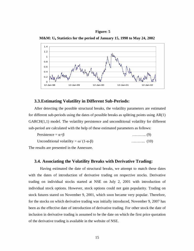
(Panel: 13 and 16). The stocks of M&M (Panel: 14) and SAIL (Panel: 18) do not show

any structural break in proximity of the date of introduction of derivative trading. The

stocks of MTNL (Panel: 15) and Tata Motors (Table: 20) do not show any structural

break in volatility at all during the period covered in this study. Stock of RIL, alike to

ITC, shows a decreased level of volatility persistence and unconditional volatility but an

increased level of adjustment coefficient after the introduction of derivative trading

(Panel: 17). In case of State Bank of India (SBI) the adjustment coefficient of the

volatility and unconditional volatility increase and persistence of volatility decreases after

the introduction of the derivative trading (Panel: 19); while in case of Tata Power (Panel:

21) the unconditional volatility decreases and the volatility persistence as well as the

speed of adjustment of volatility to new information increases.

The results obtained in this study show a mixed picture. Out of the 21 stocks, in

eight stocks no structural break was found within the stipulated time period. Out of

remaining thirteen stocks, which show structural break during the period in proximity of

introduction of derivative trading, the unconditional volatility has decreased in nine

19

stocks while in four stocks it has increased. The volatility persistence has increased in

seven stocks and decreased in six stocks. The rate of adjustment of volatility to new

information has increased in eight stocks, while it has decreased in five stocks. Therefore,

no generalisation can be made about the impact of derivative trading on volatility.

5. Conclusion:In this paper we have made an attempt to identify the structural breaks in the

volatility dynamics of twenty-one stocks using the cumulative-sum-of-squares (CUSUM)

procedure. These dates are compared with the date of introduction of derivative trading in

respective stocks to examine if any structural break is induced by the derivative trading.

If a break is observed in proximity of introduction of derivative trading, the nature of

changes in volatility persistence, rate of adjustment in volatility to news and

unconditional volatility have been analysed. We do not observe any consistent pattern in

the reaction of volatility dynamics towards introduction of derivative trading. Therefore,

it can be concluded on the basis of the results of this study that the introduction of

derivative trading has no definite implication for the volatility of underlying stocks.

Reference:Afsal E. M. and Mallikarjunappa, T. (2007), “Impact of Stock Futures on the Stock

Market Volatility”, The ICFAI Journal of Applied Finance, Vol. 13 No.9, pp.54-75.

Aggarwal, R.; Inclan, C., and Leal, R. (1999), “Volatility in Emerging Stock Markets”,Journal of Financial and Quantitative Analysis, Vol.34, No.1, pp. 33-55.

Aitken, M; Frino, A. and Jarnecic, E. (1994), “Option Listings and the Behaviour ofUnderlying Securities: Australian Evidence”, Securities Industry Research Centreof Asia-Pacific (SIRCA) Working Paper, Vol. 3, pp. 72-76.

Alexakis, P. (2007), “On the Effect of Index Futures Trading on Stock MarketVolatility”, International Research Journal of Finance and Economics, Vol. 11, 7-20.

Andreou, E. and Ghysels, E. (2002), “Detecting Multiple Breaks in Financial MarketVolatility Dynamics”, Journal of Applied Econometrics, Vol.17, No.5, pp. 579-600.

Antoniou, A. and Holmes, P. (1995), “Futures Trading, Information and Spot PriceVolatility: Evidence for the FTSE-100 Stock Index Futures Contract usingGARCH”, Journal of Banking and Finance, Vol. 19(2), pp. 117-129.

20

Bacmann, J. and M. Dubois (2002), "Volatility in Emerging Stock Markets Revisited."http://www.ssrn.com/abstract=313932.

Baillie, R. T.; Bollerslev, T. and Mikkelsen, H. O. (1996), “Fractionally IntegratedGeneralised Autoregressive Conditional Heteroskedasticity”, Journal ofEconometrics, Vol.74, No.1, pp 3-30.

Bandivadekar, S. and Ghosh, S. (2003), “Derivatives and Volatility in Indian StockMarkets”, Reserve Bank of India Occasional Papers, Vol. 24(3), pp. 187-201.

Basal, V. K.; Pruitt, S. W. and Wei, K. C. J. (1989), “An Empirical Re-examination ofthe Impact of COBE Option Initiation on the Volatility and Trading Volume ofUnderlying Equities: 1973-1986”, Financial Review, Vol. 24, pp. 19-29.

Bauer, L. (2006), “Regime Dependent Conditional Volatility in the US Equity Market”,http://papers.ssrn.com/sol3/papers.cfm?abstract_id=927044.

Bessembinder H. and Seguin, P. J. (1992), Futures Trading Activity and Stock PriceVolatility, Journal of Finance, Vol. 47, pp. 2015-2034.

Bollen, N. P.B. (1998), “A Note of the Impact of Options on Stock Return Volatility”,Journal of Banking and Finance, Vol. 22, pp. 1181-1191.

Bollerslev, T.; and Engle, R. F. (1986), “Modelling the Persistence of ConditionalVariance”, Econometric Review, Vol.5, No.1, pp 1-50.

Bollerslev, T.; Chou, R. Y. and Kroner, K. F. (1992), “ARCH Modelling in Finance: AReview of Theory and Empirical Evidence”, Journal of Econometrics, Vol.52, No.(1, 2), pp 5-59.

Brown, R. L., Durbin, J., and Evans, J. M. (1975), “Techniques for Testing the Constancy ofRegression Relationships over Time”, Journal of the Royal Statistical Society, Ser. B,Vol.37, pp 149-163.

Chou, R.Y. (1988), “Volatility Persistence and Stock Valuations: Some EmpiricalEvidence using GARCH”, Journal of Applied Econometrics, Vol.3, No.4, pp 279-294.

Conrad, J. (1989), “The Price Effect of Option Introduction”, Journal of Finance, Vo. 44,pp. 487-498.

Cox, C. C. (1976), “Futures Trading and Market Information”, Journal of PoliticalEconomy, Vol. 84, pp. 1215-37.

Danthine, J. (1978), “Information, Futures Prices and Stabilizing Speculation”, Journal ofEconomic Theory, Vol. 17, pp. 79-98.

21

Darrat, A.F., and Rahman, S. (1995), “Has Futures Trading Activity Caused Stock PriceVolatility?” Journal of Futures Markets, Vol. 15, pp. 537 – 557.

den Haan, W. J. and Levin, A. (1997), “A Practitioner’s Guide to Robust CovarianceMatrices Estimation”, in Handbook of Statistics, Vol. 15, Rao, C. R. and Maddala,G. S. (eds.), 291-341.

Diebold, F. X. (1986), “Modelling the Persistence of Conditional Variances: AComment”, Economic Review, Vol.5, No.1, pp 51-56.

Diedold, F. X. and Inoue, A. (2001), “Long Memory and Structural Change”, Journal ofEconometrics, Vol. 105, pp. 131-159.

Dueker, M. J. (1997), “Market Switching in GARCH Process and Mean Reverting StockMarket Volatility”, Journal of Business and Economic Statistics, Vol.15, No.1,pp26-34.

Edwards, Franklin R., (1988), “Does Futures Trading Increase Stock Market Volatility?”Financial Analyst Journal, Vol. 44, pp. 63-69.

Engle, R. (1982), “Autoregressive Conditional Heteroskedasticity with Estimates of theVariance of UK Inflation”, Econometrica, Vol.50, No.4, pp 987-1008.

Engle R. and Lee, G. J. (1999) “A Permanent and Transitory Component Model of StockReturn Volatility”, in R. Engle and H. White (eds.), Cointegration, Causality, andForecasting: A Festschrift in Honour of Clive W.J. Granger, Oxford UniversityPress, pp 475-497.

French, K. R; Schwert, G. W. and Stambaugh, R. F. (1987), “Expected Stock Returns andVolatility”, Journal of Financial Economics, Vol.19, pp 3-30.

Freund, S. P.; McCann, D. and Webb, G. P. (1994), “A Regression Analysis of the Effectof Option Introduction on Stock Variance”, Journal of Derivatives, Vol. 6, pp. 25-38.

Granger, C.W.J. and Hyung, N. (1999), “Occasional Structural Breaks and LongMemory”, Discussion Paper 99-14, Department of Economics, University ofCalifornia, San Diego.

Gray, S. F. (1996), “Modelling the Conditional Distribution of Interest Rates as RegimeSwitching Process”, Journal of Financial Economics, Vol.42, No.1, pp 27-62.

Gupta O.P., (2002), “Effects of Introduction of Index Futures on Stock Market Volatility:The Indian Evidence“, paper presented at Sixth Capital Market Conference, UTICapital Market, Mumbai.

22

Gulen, H. and Mayhew, S. (2000), “Stock Index Futures Trading and Volatility inInternational Equity Market”, Journal of Futures Markets, Vol. 20, pp. 661-685.

Hamilton, J. D. (1988), “Rational Expectations Econometric Analysis of Changes inRegime: An Investigation of the Term Structure of Interest Rates”, Journal ofEconomic Dynamics and Control, Vol.12 No. (2-3), pp 385-423.

Hamiltom, J. D. and Susmel, R. (1994), “Autoregressive Conditional Heteroskedasticityand Changes in Regime”, Journal of Econometrics, Vol.64, No.12, pp 307-333.

Harries, L.H. (1989), “The October 1987 S&P 500 Stock-Futures Basis”, Journal ofFinance, Vol. 1 (1), pp. 77-99.

Hass, M.; Mittnik, S. and Paolella, M. (2004), “A New Approach to Markov SwitchingGARCH Model”, Journal of Financial Econometrics, Vol.2, No.4, pp 493-530.

Herbst, A. F. and Maberly, E. D. (1992), “The Information Role of End of the DayReturns in Stock Index Futures”, Journal of Futures Markets, Vol. 12, pp. 595-601.

Inclan, C. and Tiao, G. C. (1994), “Use of Cumulative-sum-of-squares for RetrospectiveDetection of Changes of Variance”, Journal of American Statistical Association,Vol.89, No.427, pp 913-923.

Jagadeesh, N. and Subrahmanyam, A. (1993), “Liquidity effect of the Introduction ofS&P 500 Index Futures Contracts on the Underlying Stocks”, Journal of Business,Vol. 66, pp. 171-187.

Kamara, A., Millar, T. and Siegel, A. (1992), “The Effect of Futures Trading on theStability of the S&P 500 Returns”, Journal of Futures Markets, Vol. 12, pp.645-658.

Kim, S.; Cho, S. and Lee, S. (2000), “On the CUSUM Test for Parameter Changes inGARCH (1, 1) Model”, Communications in Statistics: Theory and Methods, Vol.29,No.2, pp 445-462.

Kokoszka, P. and Leipus, R. (2000), “Change-Point Estimation in ARCH Model”,Bernoulli, Vol.6, No.3, pp 513-539.

Kumar, A.; Sarin, A. and Shastri, K. (1995), “The Impact of Listing of Index Options onthe Underlying Stocks”, Pacific-Basin Finance Journal, Vol.3, pp. 303-317.

Lamoureux, C.G. and Lastrapes, W. D. (1990), “Persistence in Variance, StructuralChange and the GARCH Model”, Journal of Business and Economic Statistics,Vol.8, No.2, pp 225-234.

23

Lamoureux, C.G. and Pannikath, S.K. (1994), “Variations in Stock Returns:Asymmetries and Other Patterns”, Working Paper, John M Olin School ofBusiness, St. Louis MO.

Lee, S. and Park, S. (2001), “The CUSUM of Squares Test for Scale Changes in InfiniteOrder Moving Average Process”, Scandinavian Journal of Statistics, Vol.28, No.4,pp 625-644.

Lee, S.; Tokutsu, Y. and Meakawa, K. (), “The Residual Cusum Test for the Consistencyof Parameters in GARCH (1, 1) Models”, Hiroshima University Working Paper.

Ma, C. K. and Rao, R. P. (1988), “Information Asymmetry and Option Trading”,Financial Review, Vol. 23, pp. 39-51.

Mikosch, T. and Starica, C. (2000), “Change in Structure of Financial Time Series, LongRange Dependence and GARCH Model”, Central for Analytical Finance WorkingPaper, University of Aarhus, http://cls.dk/caf/wp/wp-58.pdf.

Narasimhan, J. and Subrahmanyam, A. (1993), “Liquidity Effects of the Introduction ofthe S&P 500 Index Futures and Contracts on the Underlying Stocks”, Journal ofBusiness, Vol. 66, pp. 171-187.

Nath, Golaka C. (2003), “Behaviour of Stock Market Volatility After Derivatives”,NSENEWS, National Stock Exchange of India, November Issue.

Peat, P. and McCorry, M. (1997), “Individual Share Futures Contract: The EconomicImpact of Their Introduction on Underlying Equity Market”, University ofTechnology Sydney, School of Finance and Economics, Working Paper No. 74,http://www.buiness.uts.edu.au./finance/.

Perron, P. (1990), “Testing For Unit Root in a Time Series With a Changing Mean”,Journal of Business and Economic Statistics, 8: pp 153-162.

Poorter M. and Dijk, D. (2004), “Testing for Changes in Volatility in HeteroskedasticityTime Series- A Further Examination”, Economic Institute Report EI 2004-38,Erasmus University Rotterdam.

Raju, M. T. and Karande, K. (2003), “Price Discovery and Volatility on NSE FuturesMarket”, SEBI Bulletin, Vol. 1(3), pp. 5-15.

Robinson, G. (1993), “The Efeect of Futures Trading on Cash Market Volatility”, Bankof England Working Paper No. 19, www.ssrn.com./Abstract id=114759.

Ross, S. A. (1989), “Information and Volatility: The No-Arbitrage Martingale Approachto Timing and Resolution Irrelevancy’, Journal of Finance, Vol. 44, pp. 1-17.

24

Saktival, P. (2007), “The Effect of Futures Trading on the Underlying Volatility:Evidence from the Indian Stock Market”, Paper presented at Fourth NationalConference on Finance & Economics, ICFAI Business School, Bangalore,December 14-15.

Samanta, P. and Samanta, P. K. (2006), “Impact of Index Futures on the Underlying SpotMarket Volatility”, ICFAI Journal of Applied Finance, Vol. 13, No. 10, pp. 52-65.

Sanso, A.; Arago, V. and Carrion, J. L. (2004) ‘Testing for Changes in the UnconditionalVariance of Financial Time Series,’ University of Barcelona Working Paper.

Schwert, G.W. and Seguin, P. J. (1990), “Heteroskedasticity in Stock Returns”, Journalof Finance, Vol.45, No.4, pp 1129-1155.

Shenbagaraman, P. (2003), “Do Futures and Options Trading Increase Stock MarketVolatility”, NSE Research Initiative paper No. 20,http://www.nseindia.com/content/reserch/paper60.pdf.

Spyrou, S. I. (2005), “Index Futures Trading and Spot Price Volatility”, Journal ofEmerging market Finance, Vol. 4, 151-167.

Stein J. C. (1987), “Information Externalities and Welfare Reducing Speculation”,Journal of Political Economy, Vol. 95, pp. 1123-1145.

Thenmozhi, M. (2002), “Futures Trading Information and Spot Price Volatility of NSE -50 Index Futures Contract”, NSE Research Initiative Paper No. 18,http://www.nseindia.com/content/reserch/paper59.pdf.

Thenmozhi, M. and Sony, T. M. (2002), “Impact of Index Derivatives on S&P CNXNifty Volatility: Information Efficiency and Expirations Effects”, ICFAI Journal ofApplied Finance, Vol. 10, pp. 36-55.

Vipul (2006), the Impact of the Introduction of the Derivatives on Underline Volatility:Evidence from India, Applied Financial Economics, Vol. 16, pp.687-694

25

Annexure

1. Volatility Breaks in ACCDate of inclusion in Nifty : before 2002Date of commencement of derivative trading : 02-07-2001

PeriodTotal

Persistence)

UnconditionalVolatility:

/(1- )02-01-1995 to 17-10-1996 2.6722 0.0798 0.7895 0.8692 20.434218-10-1996 to 05-03-2002 5.1401 0.1271 0.7897 0.9168 61.802406-03-2002 to 18-05-2004 2.1123 0.0779 0.8602 0.9381 34.113119-05-2004 to 27-02-2006 0.8276 0.0801 0.8768 0.9569 19.207428-02-2006 to 31-10-2007 3.0037 0.2937 0.5482 0.8419 18.9966

2. Volatility Breaks in Ambuja Cement

3. Volatility Breaks in Bajaj AutoDate of inclusion in Nifty : before 2002Date of commencement of derivative trading : 02-07-2001

PeriodTotal

Persistence)

UnconditionalVolatility:

/(1- )02-01-1995 to 01-10-1996 0.7331 0.1097 0.8375 0.9472 13.896202-10-1996 to13-08-2001 3.2286 0.1169 0.7752 0.8921 29.910714-08-2001 to 18-05-2004 2.6000 0.1957 0.4679 0.6636 7.728619-05-2004 to13-02-2006 1.7387 0.0471 0.8566 0.9037 18.047614-02-2006 to 31-10-2007 3.0684 0.1653 0.5588 0.7241 11.1223

4. Volatility Breaks in BHELDate of inclusion in Nifty : before 2002Date of commencement of derivative trading: 02-07-2001

PeriodTotal

Persistence)

UnconditionalVolatility:

/(1- )02-01-1995 to 28-05-1998 3.5799 0.2556 0.5843 0.8399 22.365929-05-1998 to 07-03-2002 9.1327 0.1149 0.6721 0.7871 42.886408-03-2002 to 31-10-2007 2.0388 0.1575 0.7414 0.8989 20.1737

Date of inclusion in Nifty : before 2002Date of commencement of derivative trading : 20-04-2005

PeriodTotal

Persistence)

UnconditionalVolatility:

/(1- )02-01-1995 to 08-01-1998 1.3858 0.1022 0.8510 0.9621 36.563409-01-1998 to 07-05-2001 6.4163 0.1493 0.6133 0.7626 27.027308-05-2001 to 31-10-2007 1.4357 0.0964 0.8558 0.9522 30.0299

26

5. Volatility Breaks in BPCLDate of inclusion in Nifty : before 2002Date of commencement of derivative trading: 02-07-2001

PeriodTotal

Persistence)

UnconditionalVolatility:

/(1- ) 02-01-1995 to 02-04-1998 3.2272 0.1593 0.4942 0.6535 9.3142 03-04-1998 to 19-04-2001 7.0561 0.1146 0.7911 0.9057 74.8180 20-04-2001 to 02-12-2004 5.0257 0.2000 0.5346 0.7346 18.9364 03-12-2004 to 31-10-2007 2.5205 0.0902 0.7976 0.8878 22.4667

6. Volatility Breaks in CiplaDate of inclusion in Nifty : Before 2002Date of commencement of derivative trading: 02-07-2001

PeriodTotal

Persistence)

UnconditionalVolatility:

/(1- )02-01-1995 to 27-02-1996 5.1531 0.2368 0.50063 0.7375 19.627228-02-1996 to 18-12-1998 3.2377 0.2148 0.51033 0.7251 11.777319-12-1998 to 22-10-2001 3.7717 0.0726 0.89078 0.9634 103.024123-10-2001 to 25-04-2003 1.5358 0.1024 0.50407 0.6065 3.902926-04-2003 to 31-10-2007 3.0240 0.1547 0.55661 0.7113 10.4736

7. Volatility Breaks in Dr. Reddy

8. Volatility Breaks in GlaxoDate of inclusion in Nifty : Before 2002Date of commencement of derivative trading: : 01-07-2005

PeriodTotal

Persistence)

UnconditionalVolatility:

/(1- )02-01-1995 to 11-11-1997 2.8904 0.1777 0.1367 0.3143 4.215512-11-1997 to 17-12-1999 6.0813 0.2566 0.1054 0.3621 9.532617-12-1999 to 05-06-2000 12.0360 0.1773 0.2942 0.4715 22.771806-06-2000 to 21-05-2002 3.6969 0.2771 0.3878 0.6649 11.031422-05-2002 to 31-10-2007 1.5725 0.1276 0.7649 0.8925 14.6324

Date of inclusion in Nifty : Before 2002Date of commencement of derivative trading: 02-07-2001

PeriodTotal

Persistence)

UnconditionalVolatility:

/(1- )02-01-1995 to 17-03-1998 2.1294 0.2210 0.6338 0.8548 14.664618-03-1998 to 21-06-2000 6.5563 0.1287 0.7772 0.9059 69.651722-06-2000 to 31-05-2004 5.1207 0.2005 0.0682 0.2687 7.001901-06-2004 to 31-10-2007 0.8829 0.0318 0.9574 0.9892 81.4470

27

9. Volatility Breaks in GrasimDate of inclusion in Nifty : Before 2002Date of commencement of derivative trading : 02-07-2001

PeriodTotal

Persistence)

UnconditionalVolatility:

/(1- )02-01-1995 to 03-02-1998 2.0851 0.1144 0.3234 0.4378 3.708704-02-1998 to 26-05-2000 6.4494 0.0864 0.8591 0.9455 118.229427-05-2000 to 31-12-2001 5.9509 0.3074 0.2615 0.5690 13.806201-01-2002 to 31-10-2007 1.1593 0.1685 0.7733 0.9419 19.9402

10. Volatility Breaks in HPCLDate of inclusion in Nifty : Before 2002Date of commencement of derivative trading : 02-07-2001

PeriodTotal

Persistence)

UnconditionalVolatility:

/(1- )02-01-1995 to 10-05-1995 6.1886 0.0111 0.8245 0.8356 37.643611-05-1995 to 29-05-1998 1.8622 0.1950 0.4607 0.6557 5.409030-05-1998 to12-01-2001 9.4250 0.3387 0.1072 0.4459 17.009613-01-2001 to 06-08-2002 1.9543 0.0891 0.8883 0.9774 86.513907-08-2002 to 31-10-2007 2.3208 0.1089 0.8484 0.9573 54.3013

11. Volatility Breaks in HULDate of inclusion in Nifty : Before 2002Date of commencement of derivative trading : 02-07-2001

PeriodTotal

Persistence)

UnconditionalVolatility:

/(1- )02-01-1995 to 25-04-1997 0.9545 0.1520 0.6730 0.8250 5.452626-04-1997 to 10-10-2001 2.1280 0.1027 0.8372 0.9399 35.389711-10-2001 to 02-07-2003 0.9774 0.0991 0.8447 0.9437 17.366203-07-2003 to 31-10-2007 2.6968 0.1359 0.6235 0.7594 11.2087

12. Volatility Breaks in ITCDate of inclusion in Nifty : Before 2002Date of commencement of derivative trading : 02-07-2001

PeriodTotal

Persistence)

UnconditionalVolatility:

/(1- )02-01-1995 to 02-11-2001 3.4298 0.0689 0.8795 0.9484 66.418103-11-2001 to 02-09-2005 1.6997 0.1810 0.6055 0.7865 7.961703-09-2005 to 31-10-2007 2.2541 0.0878 0.8126 0.9003 22.6129

28

13. Volatility Breaks in L&TDate of inclusion in Nifty : Before 2002Date of commencement of derivative trading : 02-07-2001

PeriodTotal

Persistence)

UnconditionalVolatility:

/(1- )02-01-1995 to 30-04-1998 2.4064 0.1320 0.7277 0.8597 17.154501-05-1998 to 25-07-2000 7.3246 0.0824 0.8334 0.9159 87.052526-07-2000 to 09-11-2001 5.9836 0.1232 0.6126 0.7358 22.648010-11-2001 to 23-05-2003 0.7583 0.0186 0.9670 0.9856 52.659224-05-2003 to 31-10-2007 1.8871 0.1601 0.7634 0.9235 24.6802

14. Volatility Breaks in M&MDate of inclusion in Nifty : Before 2002Date of commencement of derivative trading : 02-07-2001

PeriodTotal

Persistence)

UnconditionalVolatility:

/(1- )02-01-1995 to 14-01-1998 3.5084 0.1041 0.6018 0.7059 11.928715-01-1998 to 24-05-2002 6.0605 0.1324 0.7527 0.8851 52.736325-05-2002 to 31-10-2007 1.6448 0.0871 0.8717 0.9588 39.9231

15. Volatility Breaks in MTNLDate of inclusion in Nifty : Before 2002Date of commencement of derivative trading : 02-07-2001No structural break in volatility is detected

16. Volatility Breaks in Reliance EnergyDate of inclusion in Nifty : before 2002Date of commencement of derivative trading : 12-03-2004

PeriodTotal

Persistence)

UnconditionalVolatility:

/(1- )02-01-1995 to 01-04-1999 4.6660 0.1367 0.6092 0.7459 18.360802-04-1999 to 30-05-2001 6.3253 0.1646 0.6722 0.8368 38.764931-05-2001 to 06-06-2003 2.0174 0.1347 0.6117 0.7464 7.954707-06-2003 to 18-05-2004 5.9502 0.5140 0.0655 0.4485 10.790019-05-2004 to 31-10-2007 2.1141 0.2109 0.6901 0.9010 21.3477

29

17. Volatility Breaks in RILDate of inclusion in Nifty : before 2002Date of commencement of derivative trading : 29-11-2001

PeriodTotal

Persistence)

UnconditionalVolatility:

/(1- )02-01-1995 to 20-11-2001 3.6022 0.2186 0.6355 0.8541 24.689621-11-2001 to 31-10-2007 2.1473 0.2527 0.4844 0.7371 8.1664

18. Volatility Breaks in SAILDate of inclusion in Nifty : 04-08-2003Date of commencement of derivative trading: 15-09-2006

PeriodTotal

Persistence)

UnconditionalVolatility:

/(1- )02-01-1995 to 24-11-1997 4.2023 0.2113 0.6260 0.8374 5.018625-11-1997 to 05-04-2000 20.2690 0.4358 0.0237 0.4595 35.500506-04-2000 to 09-07-2004 3.2230 0.2363 0.7418 0.9780 3.295510-07-2004 to 31-10-2007 3.1393 0.1815 0.7367 0.9182 3.4191

19. Volatility Breaks in SBIDate of inclusion in Nifty: Before 2002Date of commencement of derivative trading: 02-07-2001

PeriodTotal

Persistence)

UnconditionalVolatility:

/(1- )02-01-1995 to 28-02-2002 0.8837 0.0667 0.8999 0.9666 26.425101-03-2002 to 19-12-2003 2.9875 0.1090 0.8261 0.9351 45.997020-12-2003 to 19-05-2004 6.0329 0.3889 0.2063 0.5952 14.902020-05-2004 to 31-10-2007 1.8995 0.0495 0.9143 0.9637 52.3412

20. Volatility Breaks in Tata MotersDate of inclusion in Nifty : before 2002Date of commencement of derivative trading : 26-12-2003No structural break in volatility is detected

21. Volatility Breaks in Tata PowerDate of inclusion in Nifty : before 2002Date of commencement of derivative trading : 02-07-2001

PeriodTotal

Persistence)

UnconditionalVolatility:

/(1- )02-01-1995 to 26-03-1999 4.1018 0.2074 0.1945 0.4019 6.857927-03-1999 to 04-03-20002 6.9024 0.1175 0.7107 0.8282 40.176905-03-2002 to 31-10-2007 1.4513 0.1572 0.7841 0.9413 24.7026