56
Deriving Priority Areas for Investment A technical report to accompany the Draft NSW Biodiversity Strategy
Deriving Priority Areas for Investment
A technical report to accompany the Draft NSW Biodiversity Strategy
Cover photographs: Main photograph: D. Barnes, Replanting seedlings, © NSW DPI Image Library. Right-hand photographs, from top to bottom: NASA, The Earth seen from Apollo 17, 2005, public domain image NASA, Australia Satellite Plan, taken on 19th May 2005, public domain image DECCW, GIS map of NSW using DECCW data, 2010 DECCW, Satellite imagery of an area in Northern NSW, accessed 2010, © Digital aerial imagery – NSW Land and Property Management Authority, Panorama Avenue, Bathurst.
Published by:
Department of Environment, Climate Change and Water NSW 59–61 Goulburn Street; PO Box A290 Sydney South 1232 Phone: (02) 9995 5000 (switchboard) Phone: 131 555 (environment information and publications requests) Phone: 1300 361 967 (national parks information and publications requests) Fax: (02) 9995 5999 TTY: (02) 9211 4723 Email: [email protected] Website: www.environment.nsw.gov.au
DECCW is pleased to allow this material to be reproduced in whole or in part, provided the meaning is unchanged, and its source, publisher and authorship are acknowledged.
ISBN 978-1-74232-982-6 DECCW 2010/878 November 2010
Printed on recycled paper
Contents
1 Introduction ............................................................................................................... 4
2 Identifying investment priorities .............................................................................. 4
2.1 Criteria for identifying Priority Areas ...........................................................................4
2.2 Features of the Priority Area map ................................................................................5
3 Overview of the methods used to identify Priority Areas ...................................... 7
4 Building a model to locate Priority Areas ............................................................... 9
Step A: Dividing NSW vegetation into grid-cells ...................................................................9
Step B: Forming Vegetation Groups ...................................................................................10
Step C: Calculating condition and connectivity scores .......................................................13
Step D: Calculating the biodiversity index of each Vegetation Group ................................17
Step E: Calculating the total biodiversity index for New South Wales ................................19
Step F: Calculating the marginal biodiversity contribution of Vegetation Groups ...............19
Step G: Calculating the priority scores ................................................................................20
Summary of Steps A to G ....................................................................................................21
5 Creating the initial map showing relative priorities .............................................. 25
5.1 Modifications to the initial map ..................................................................................25
5.2 Ecosystems excluded from the Priority Area map ....................................................26
6 The final Priority Area map..................................................................................... 30
6.1 Viewing the map ........................................................................................................32
7 Relating the Priority Areas to the ecosystems of New South Wales ................... 33
7.1 Further examination of Priority Areas ........................................................................34
8 Clusters of Priority Areas ....................................................................................... 35
9 Assigning responsibilities: who manages the Priority Areas? ........................... 38
10 Using the maps: how to find Priority Areas ‛on the ground’ ............................... 41
10.1 Should all high Priority Areas be actively managed for biodiversity?........................41
10.2 How should the map be used? ..................................................................................42
11 References .............................................................................................................. 43
Appendix 1: Categories of Crown Reserves with a conservation purpose .................. 45
Appendix 2: Aggregating the BDI values for Vegetation Groups into a single BDI for New South Wales ............................................................................. 47
Appendix 3: Calculating the fragmentation level of ecosystem types ........................... 49
Appendix 4: Extent of Priority Areas in each ecosystem type (hectares) by CMA and land tenure .................................................................................................... 52
4 Draft NSW Biodiversity Strategy: Technical Paper
1 Introduction This technical report provides an explanation of the investment priorities identified in the Draft NSW Biodiversity Strategy 2010–2015 (referred to in this report as ‘the Draft Strategy’).
In particular, this report describes:
• the methods used to develop the map of Priority Areas
• the additional steps taken to classify Priority Areas according to their ecosystem type and tenure
• details on how the map of Priority Areas can be used and interpreted.
2 Identifying investment priorities In 2009, the Department of Environment, Climate Change and Water NSW (DECCW) established an internal committee to develop a set of criteria that could be used for identifying Priority Areas at a state scale for investment in biodiversity management.
2.1 Criteria for identifying Priority Areas Using the best available science, it was determined that investment should be directed towards areas with the following characteristics:
Criteria A: Sites that are in ‘good’ condition
Priority Areas for investment are intended to represent the best remaining examples of degraded vegetation communities. With that in mind, the Draft Strategy assigns a higher priority status to sites that are in better condition. However, once other attributes are taken into account in the analysis, Priority Areas can range in condition from ‘moderate’ to ‘very good’.
The biodiversity benefits of investing in vegetation of ‘moderate to very good condition’ are likely to be relatively high, compared with the cost. This is largely because vegetation in moderate to very good condition already has important biodiversity values that can be maintained or enhanced for a modest investment, and management actions to address threats are likely to be more successful than management of areas in low condition.
‘Degraded’ vegetation is not considered a high priority for investment because of the prohibitive costs of management required for the large-scale improvement of this vegetation compared with the likely gain for biodiversity. However, in a small number of cases, degraded areas may be identified on the Priority Area map if they are part of an extremely degraded or over-cleared type of vegetation. Site assessment is vital for identifying sites where investment is appropriate (see section 10 for further discussion).
Deriving Priority Areas for Investment 5
Criteria B: Sites that are ‘well-connected’ with other areas of native vegetation
Science tells us that well-connected landscapes retain more biodiversity over time and are more resilient to threats (such as weed invasion) than fragmented landscapes. Connected landscapes would cope better in a changing climate. Therefore, well-connected vegetation is a priority for investment.
Criteria C: Sites that contain ‘floristically distinctive’ vegetation
Vegetation communities that are particularly ‘distinctive’ in terms of their species composition but are not well-conserved are an obvious priority for maximising biodiversity outcomes. This is particularly true for communities that are highly cleared because the species they contain are not well-conserved in other vegetation communities.
Criteria D: Vegetation communities that have been ‘highly cleared’, ‘degraded’ and/or ‘fragmented’
Some types of vegetation have experienced higher rates of clearing in the past than others. Highly cleared types of vegetation are a priority for investment because:
• further pressure would lead to disproportionately high rates of biodiversity loss
• investment in management would lead to high rates of biodiversity retention
• they are generally located in landscapes also facing greater future pressures.
Criteria A to C relate to the characteristics of native vegetation at the site scale, whereas Criteria D relates to the broader vegetation community type to which a site belongs. In making this distinction, we are targeting sites that are in good condition, well-connected and distinctive but that belong to a vegetation community that has been highly cleared, degraded and/or fragmented in the past.
2.2 Features of the Priority Area map The Priority Area map (Figure 1, Part A of the Draft Strategy) and the model used to derive it have been designed to identify areas that satisfy the four criteria detailed above. The result is a map that identifies the best remaining examples of native vegetation belonging to ecosystems that have experienced high rates of past clearing, degradation and/or fragmentation.
The Priority Area map is not a high conservation value (HCV) map. Many of the ‘best’ areas for biodiversity in New South Wales have not been identified on the Priority Area map because they contain vegetation that is already well-conserved.
The Priority Area map is not a ‘restoration’ map. It does not identify high Priority Areas for revegetation or intensive restoration in sites with very low biodiversity value or in very degraded landscapes. Rather, it identifies areas that have existing value for biodiversity, where management actions will enhance or maintain those values.
6 Draft NSW Biodiversity Strategy: Technical Paper
The Priority Areas identified on the map do not replace but complement priority sites that have been identified in other DECCW programs for threatened species recovery or in threat abatement programs (see Part A of the Draft Strategy). Priority sites in these programs may occur in locations that are different to areas identified as Priority Areas on the Draft Strategy map. It is expected that investment in these priority threat abatement and recovery plan sites will continue. The Draft Strategy includes an action to revise the Priorities Action Statement under the Threatened Species Conservation Act 1995 (TSC Act) to prioritise threatened species. This will inform the allocation of investment in recovery programs and complement the Priority Areas for native vegetation programs.
Priorities for investment in aquatic biodiversity are not mapped in the Draft Strategy (apart from Forested Wetlands; see Part B of the Draft Strategy) and are described in the text. Aquatic Priority Areas have been identified by experts and are based on existing programs of work (see Part B of the Draft Strategy). Developing a spatial prioritisation for aquatic ecosystems is a key action in the Draft Strategy (see Part A of the Draft Strategy).
Similarly, Priority Areas for Arid Shrublands could not be mapped using the standard Biodiversity Forecasting Toolkit (BFT) approach (see section 5 for further discussion). Instead, an estimated 10% of all Arid Shrublands has been given priority status for investment, wherever native vegetation would significantly benefit from reduced total grazing pressure (10% of extant vegetation is the average proportion of all formations that are a priority for investment).
The map is tenure-blind. Priority Areas occur on public and private land and management actions on private land would only occur if the landowner agreed to participate.
A greater extent of Priority Area has been identified on the map than can currently be invested in over the five-year life of the Draft Strategy. The map therefore provides flexibility to land managers and regional planning bodies by presenting a range of options that can be chosen from when investing in Priority Areas. For instance, the map provides a range of Priority Area options for Catchment Management Authorities (CMAs) to use for private land conservation programs.
Climate change: Investing in Priority Areas enhances investment in climate change adaptation
Climate change has the potential to cause a significant loss of biodiversity from New South Wales. This loss can be minimised by improving the connectivity of vegetation to allow species to move along environmental gradients in response to changing climatic conditions. The Priority Areas identified in the Draft Strategy are located within well-connected landscapes. Investing in Priority Areas will improve the adaptability and resilience of these well-connected landscapes and the species they contain, in the face of future climate change impacts.
(continued)
Deriving Priority Areas for Investment 7
The Great Eastern Ranges (GER) initiative is being implemented by a range of partners, including DECCW, as a continental-scale corridor to assist in biodiversity adaptation to climate change. Priority Areas identified in the Draft Strategy overlap closely with the key areas targeted in the GER initiative.
The Draft Strategy maximises ecosystem diversity, and in turn, species diversity, in its choice of Priority Areas. All native species possess traits that help them to respond to changes in the environment, and all ecosystems will respond differently to environmental change. Investing in a greater diversity of species and ecosystems will increase the range of ‘responses’ available to living systems in the event of large-scale changes such as climate change. This is another way that investment in Priority Areas will lead to an improvement in climate change adaptation.
DECCW recently released a plan to address Priorities for Biodiversity Adaptation to Climate Change (DECCW 2010) in response to the listing of ‘Anthropogenic Climate Change’ as a key threatening process under the TSC Act. The plan identifies a range of actions that will be carried out by DECCW between 2010 and 2015 to improve the capacity of ecosystems to adapt to a changing climate. The plan focuses on developing a greater understanding of the likely impacts of climate change on biodiversity and on developing strategies to minimise such impacts. Among these are the identification of ‘refugia’ (important sites for ‘retreating’ species) and important migration corridors, particularly at the state or continent scale. Once this information has been collected, it can be used to further integrate climate change considerations into priorities for biodiversity investment.
As information about the potential impacts of climate change on biodiversity continues to grow, techniques for incorporating climate change into prioritisation processes will also multiply.
3 Overview of the methods used to identify Priority Areas
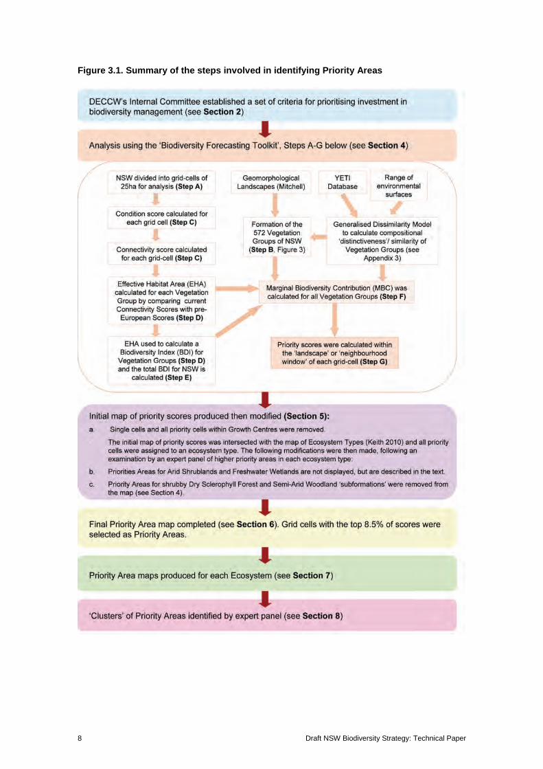
The model used to identify Priority Areas is based on DECCW’s Biodiversity Forecasting Toolkit (BFT) (DEC 2006), a decision-support system that has been developed and refined over a number of years to map biodiversity management priorities in New South Wales. The Priority Area map is based on this BFT model, with a number of additional refinements. Figure 3.1 provides an overview of the steps taken to produce the Priority Area map for the Draft Strategy.
8 Draft NSW Biodiversity Strategy: Technical Paper
Figure 3.1. Summary of the steps involved in identifying Priority Areas
Deriving Priority Areas for Investment 9
4 Building a model to locate Priority Areas
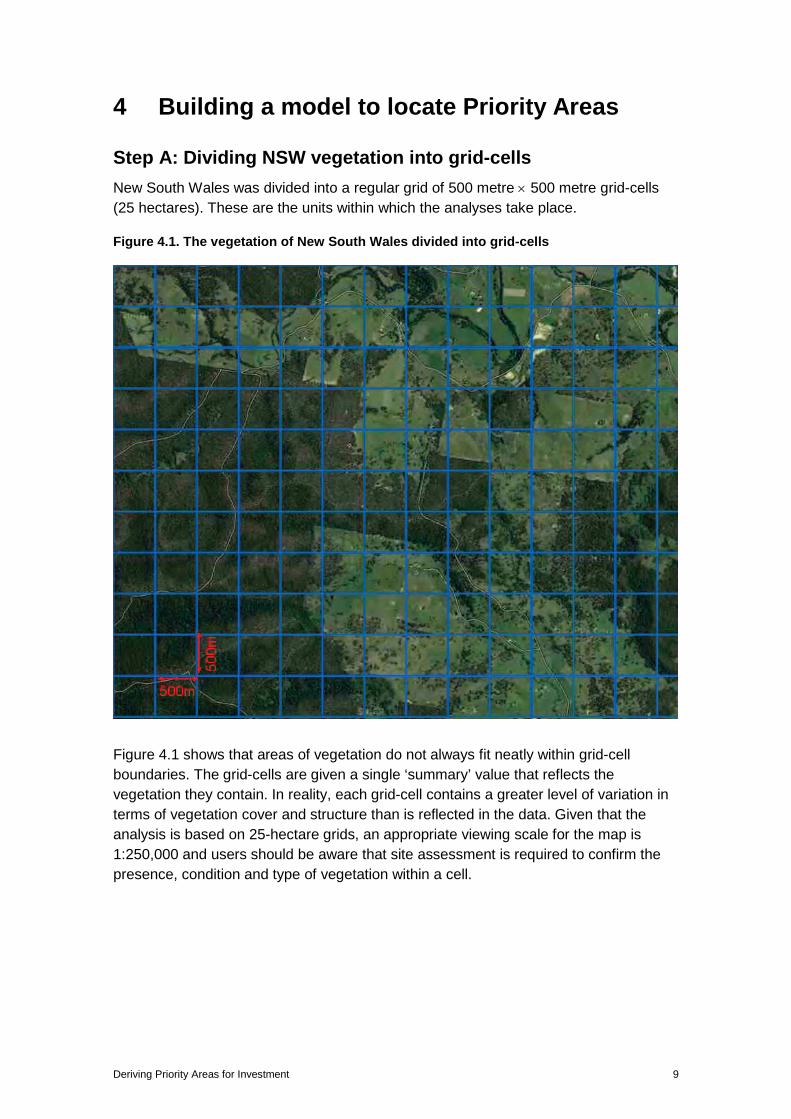
Step A: Dividing NSW vegetation into grid-cells New South Wales was divided into a regular grid of 500 metre × 500 metre grid-cells (25 hectares). These are the units within which the analyses take place.
Figure 4.1. The vegetation of New South Wales divided into grid-cells
Figure 4.1 shows that areas of vegetation do not always fit neatly within grid-cell boundaries. The grid-cells are given a single ‘summary’ value that reflects the vegetation they contain. In reality, each grid-cell contains a greater level of variation in terms of vegetation cover and structure than is reflected in the data. Given that the analysis is based on 25-hectare grids, an appropriate viewing scale for the map is 1:250,000 and users should be aware that site assessment is required to confirm the presence, condition and type of vegetation within a cell.
10 Draft NSW Biodiversity Strategy: Technical Paper
Step B: Forming Vegetation Groups Vegetation Groups were formed from the 572 geomorphology units that have been mapped statewide by Mitchell (2002). Data on plant species composition for each unit was gathered from field data stored in DECCW’s YETI database. Survey data was not available for all grid-cells; therefore, a range of environmental attributes was used to ‘fill in the gaps’ when characterising the floristic composition of different Vegetation Groups (Logan et al. 2009; see Appendix 2 for more details).
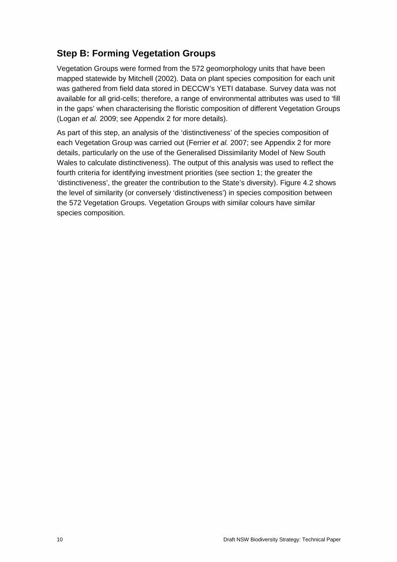
As part of this step, an analysis of the ‘distinctiveness’ of the species composition of each Vegetation Group was carried out (Ferrier et al. 2007; see Appendix 2 for more details, particularly on the use of the Generalised Dissimilarity Model of New South Wales to calculate distinctiveness). The output of this analysis was used to reflect the fourth criteria for identifying investment priorities (see section 1; the greater the ‘distinctiveness’, the greater the contribution to the State’s diversity). Figure 4.2 shows the level of similarity (or conversely ‘distinctiveness’) in species composition between the 572 Vegetation Groups. Vegetation Groups with similar colours have similar species composition.
Deriving Priority Areas for Investment 11
Figure 4.2. Compositional similarity for the 572 Vegetation Groups of New South Wales
(a) Existing vegetation
(b) Modelled pre-European vegetation
12 Draft NSW Biodiversity Strategy: Technical Paper
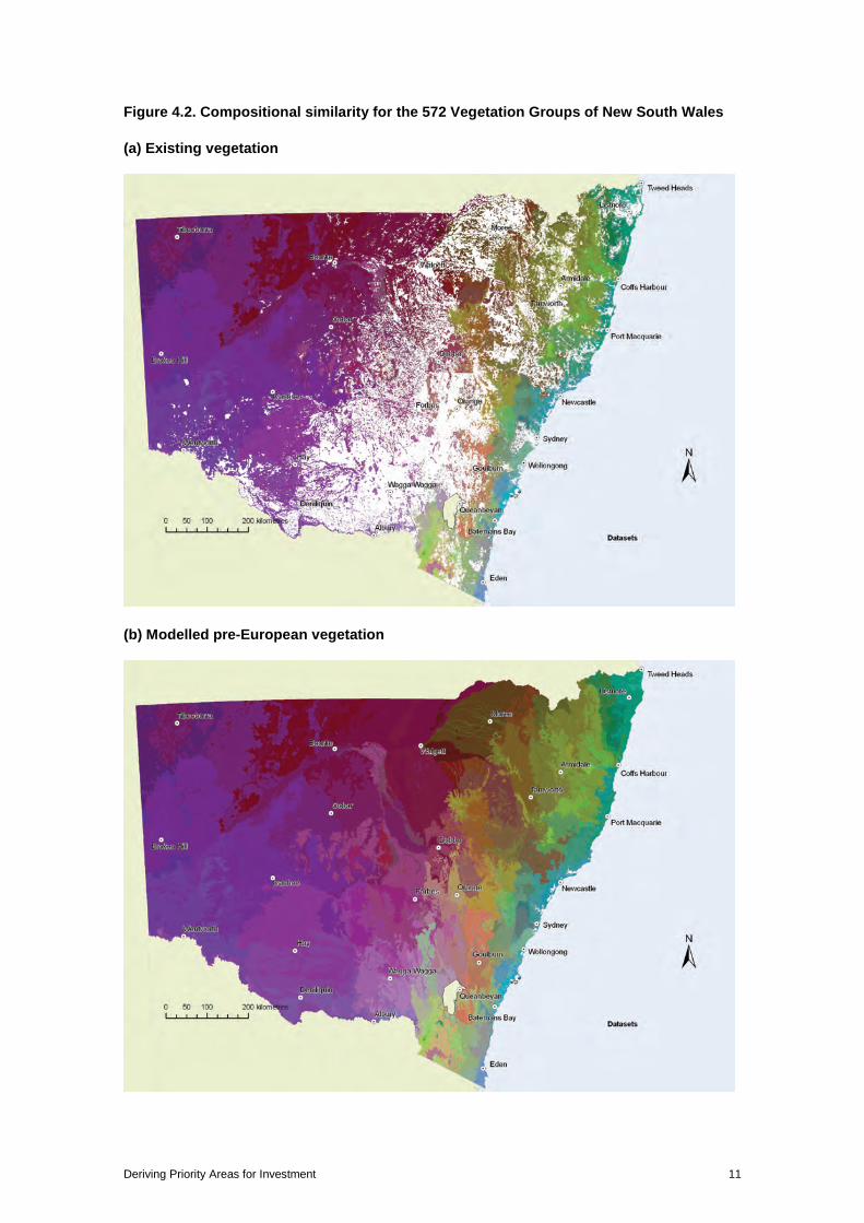
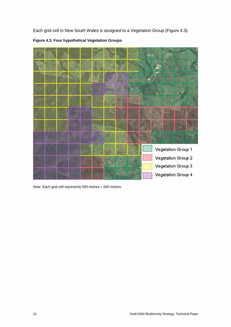
Each grid-cell in New South Wales is assigned to a Vegetation Group (Figure 4.3).
Figure 4.3. Four hypothetical Vegetation Groups
Note: Each grid-cell represents 500 metres × 500 metres.
Deriving Priority Areas for Investment 13
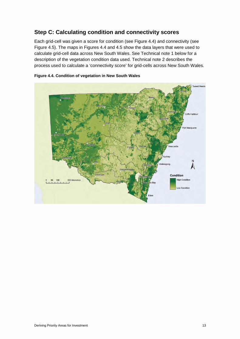
Step C: Calculating condition and connectivity scores Each grid-cell was given a score for condition (see Figure 4.4) and connectivity (see Figure 4.5). The maps in Figures 4.4 and 4.5 show the data layers that were used to calculate grid-cell data across New South Wales. See Technical note 1 below for a description of the vegetation condition data used. Technical note 2 describes the process used to calculate a ‘connectivity score’ for grid-cells across New South Wales.
Figure 4.4. Condition of vegetation in New South Wales
14 Draft NSW Biodiversity Strategy: Technical Paper
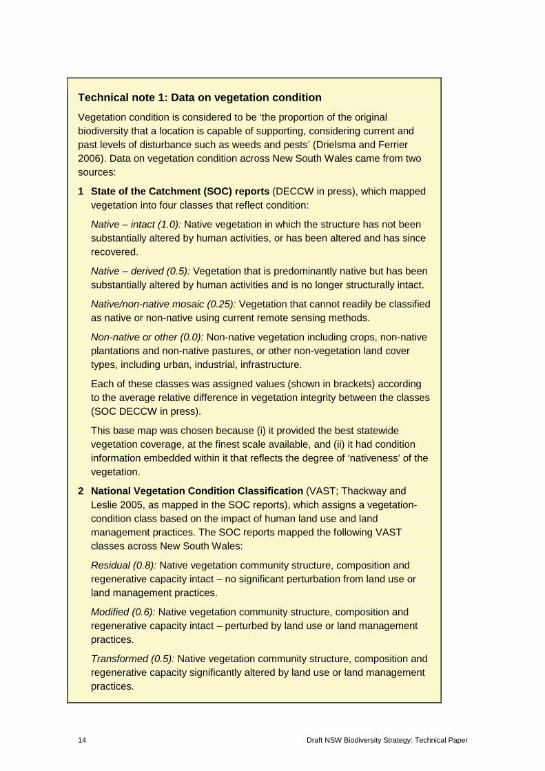
Technical note 1: Data on vegetation condition
Vegetation condition is considered to be ‘the proportion of the original biodiversity that a location is capable of supporting, considering current and past levels of disturbance such as weeds and pests’ (Drielsma and Ferrier 2006). Data on vegetation condition across New South Wales came from two sources:
1 State of the Catchment (SOC) reports (DECCW in press), which mapped vegetation into four classes that reflect condition:
Native – intact (1.0): Native vegetation in which the structure has not been substantially altered by human activities, or has been altered and has since recovered.
Native – derived (0.5): Vegetation that is predominantly native but has been substantially altered by human activities and is no longer structurally intact.
Native/non-native mosaic (0.25): Vegetation that cannot readily be classified as native or non-native using current remote sensing methods.
Non-native or other (0.0): Non-native vegetation including crops, non-native plantations and non-native pastures, or other non-vegetation land cover types, including urban, industrial, infrastructure.
Each of these classes was assigned values (shown in brackets) according to the average relative difference in vegetation integrity between the classes (SOC DECCW in press).
This base map was chosen because (i) it provided the best statewide vegetation coverage, at the finest scale available, and (ii) it had condition information embedded within it that reflects the degree of ‘nativeness’ of the vegetation.
2 National Vegetation Condition Classification (VAST; Thackway and Leslie 2005, as mapped in the SOC reports), which assigns a vegetation-condition class based on the impact of human land use and land management practices. The SOC reports mapped the following VAST classes across New South Wales:
Residual (0.8): Native vegetation community structure, composition and regenerative capacity intact – no significant perturbation from land use or land management practices.
Modified (0.6): Native vegetation community structure, composition and regenerative capacity intact – perturbed by land use or land management practices.
Transformed (0.5): Native vegetation community structure, composition and regenerative capacity significantly altered by land use or land management practices.
Deriving Priority Areas for Investment 15
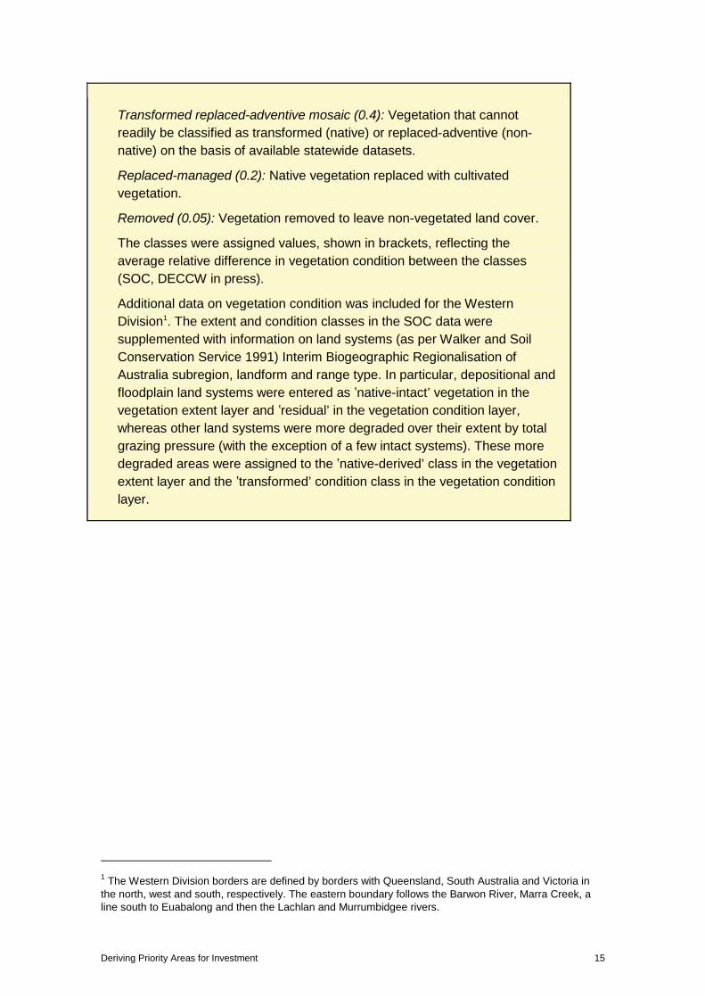
Transformed replaced-adventive mosaic (0.4): Vegetation that cannot readily be classified as transformed (native) or replaced-adventive (non-native) on the basis of available statewide datasets.
Replaced-managed (0.2): Native vegetation replaced with cultivated vegetation.
Removed (0.05): Vegetation removed to leave non-vegetated land cover.
The classes were assigned values, shown in brackets, reflecting the average relative difference in vegetation condition between the classes (SOC, DECCW in press).
Additional data on vegetation condition was included for the Western Division1. The extent and condition classes in the SOC data were supplemented with information on land systems (as per Walker and Soil Conservation Service 1991) Interim Biogeographic Regionalisation of Australia subregion, landform and range type. In particular, depositional and floodplain land systems were entered as ‛native-intact’ vegetation in the vegetation extent layer and ‛residual’ in the vegetation condition layer, whereas other land systems were more degraded over their extent by total grazing pressure (with the exception of a few intact systems). These more degraded areas were assigned to the ‛native-derived’ class in the vegetation extent layer and the ‛transformed’ condition class in the vegetation condition layer.
1 The Western Division borders are defined by borders with Queensland, South Australia and Victoria in the north, west and south, respectively. The eastern boundary follows the Barwon River, Marra Creek, a line south to Euabalong and then the Lachlan and Murrumbidgee rivers.
16 Draft NSW Biodiversity Strategy: Technical Paper
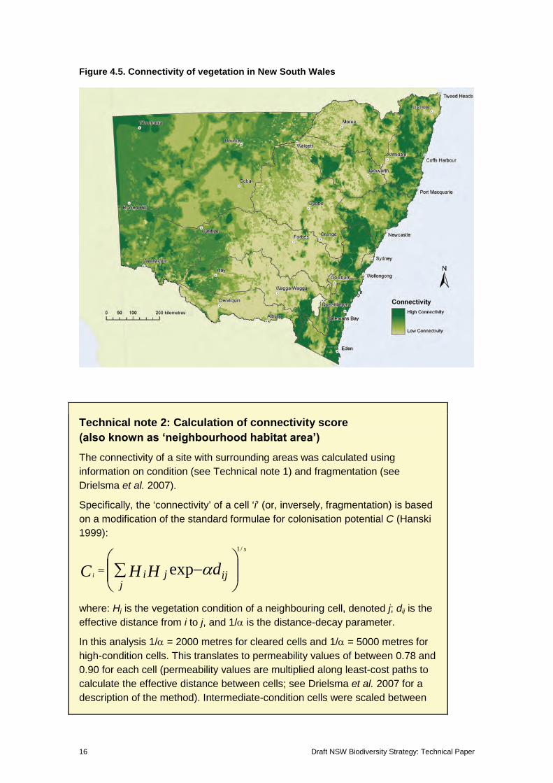
Figure 4.5. Connectivity of vegetation in New South Wales
Technical note 2: Calculation of connectivity score (also known as ‘neighbourhood habitat area’)
The connectivity of a site with surrounding areas was calculated using information on condition (see Technical note 1) and fragmentation (see Drielsma et al. 2007).
Specifically, the ‘connectivity’ of a cell ‘i’ (or, inversely, fragmentation) is based on a modification of the standard formulae for colonisation potential C (Hanski 1999):
−∑= ij
jji dHHC
s
i αexp/1
where: Hj is the vegetation condition of a neighbouring cell, denoted j; dij is the effective distance from i to j, and 1/α is the distance-decay parameter.
In this analysis 1/α = 2000 metres for cleared cells and 1/α = 5000 metres for high-condition cells. This translates to permeability values of between 0.78 and 0.90 for each cell (permeability values are multiplied along least-cost paths to calculate the effective distance between cells; see Drielsma et al. 2007 for a description of the method). Intermediate-condition cells were scaled between
Deriving Priority Areas for Investment 17
these values. The s parameter acts to balance the influence of fragmentation and condition within the BFT. In this analysis, s = 4. This meant that locations supporting over-cleared vegetation were not as ‘penalised’ (given lower priority) for being part of small, isolated or fragmented patches, as would otherwise be the case if s were a lower value.
This connectivity measure incorporates the condition of the ‘focal’ cell of interest, with the amount of vegetation, its condition and the connectivity of habitat within the focal cell’s neighbourhood. The neighbourhood of each cell is defined by a 51 × 51 cell ‛neighbourhood window’ (25.5 kilometres × 25.5 kilometres) (see Technical note 4).
Step D: Calculating the biodiversity index of each Vegetation Group The biodiversity index (BDI) of each Vegetation Group is a function of its remaining extent, condition and fragmentation. Further, it is a measure of the proportion of the original species within the community that is expected to persist, given the relationship that exists between the area of habitat and the number of species that habitat can support.
The steps taken to derive the BDI are:
1 Calculate a condition score for each grid-cell (see Technical note 1)
2 Use the condition score of each grid-cell (from Step 1), combined with data on condition and clearing within the surrounding landscape to calculate a connectivity score for the grid-cell (see Technical note 2).
3 Use the connectivity score (also known as ‘neighbourhood habitat area’, Drielsma et al. 2007) to calculate an effective habitat area (EHA) for each grid-cell. This is calculated as the current connectivity score of the cell divided by its pre-European connectivity score. The EHA of each Vegetation Group is calculated by summing the EHA scores of each grid-cell within that group.
4 Calculate the BDI (see Technical note 3) by comparing existing EHA with pre-European EHA for each Vegetation Group.
Technical note 3: The biodiversity index of each Vegetation Group
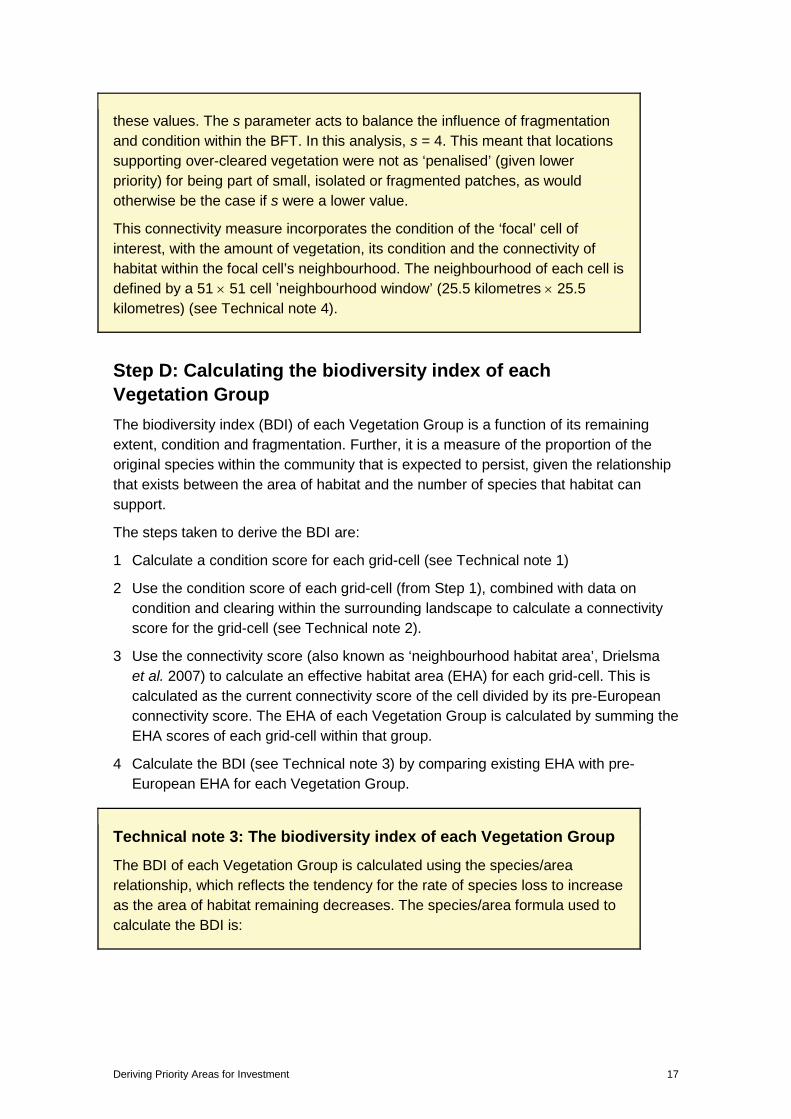
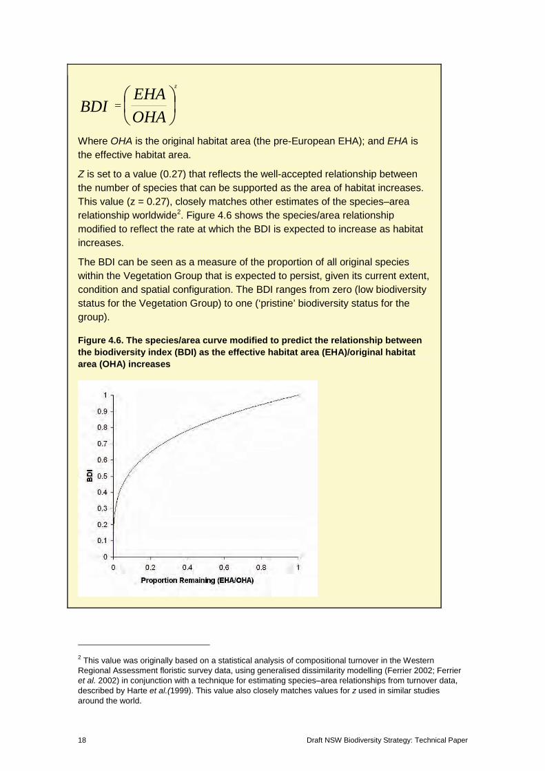
The BDI of each Vegetation Group is calculated using the species/area relationship, which reflects the tendency for the rate of species loss to increase as the area of habitat remaining decreases. The species/area formula used to calculate the BDI is:
18 Draft NSW Biodiversity Strategy: Technical Paper
=OHAEHA
BDIz
Where OHA is the original habitat area (the pre-European EHA); and EHA is the effective habitat area.
Z is set to a value (0.27) that reflects the well-accepted relationship between the number of species that can be supported as the area of habitat increases. This value (z = 0.27), closely matches other estimates of the species–area relationship worldwide2. Figure 4.6 shows the species/area relationship modified to reflect the rate at which the BDI is expected to increase as habitat increases.
The BDI can be seen as a measure of the proportion of all original species within the Vegetation Group that is expected to persist, given its current extent, condition and spatial configuration. The BDI ranges from zero (low biodiversity status for the Vegetation Group) to one (‘pristine’ biodiversity status for the group).
Figure 4.6. The species/area curve modified to predict the relationship between the biodiversity index (BDI) as the effective habitat area (EHA)/original habitat area (OHA) increases
2 This value was originally based on a statistical analysis of compositional turnover in the Western Regional Assessment floristic survey data, using generalised dissimilarity modelling (Ferrier 2002; Ferrier et al. 2002) in conjunction with a technique for estimating species–area relationships from turnover data, described by Harte et al.(1999). This value also closely matches values for z used in similar studies around the world.
Deriving Priority Areas for Investment 19
Step E: Calculating the total biodiversity index for New South Wales The BDI values for each Vegetation Group were aggregated into an overall BDI for New South Wales (the NSW BDI). If each Vegetation Group was completely separate and different from one another, then the values could simply be summed to a maximum value of 572 (i.e. the number of Vegetation Groups in New South Wales). However, given the high degree of overlap in species composition, a more complex analysis of the relative distinctiveness of each group was needed (see Appendix 3). This is because more ‘distinctive’ Vegetation Groups contribute more to the biodiversity of New South Wales.
Step F: Calculating the marginal biodiversity contribution of Vegetation Groups The marginal biodiversity contribution (MBC) score is a measure of the contribution that is made to the NSW BDI by improving the overall biodiversity status of a Vegetation Group. The MBC takes into account the ‘distinctiveness’ of a Vegetation Group compared with other, well-conserved Vegetation Groups. As such, the MBC is a function of the remaining extent, condition, fragmentation and distinctiveness of a Vegetation Group.
The ‘distinctiveness’ of Vegetation Groups is a crucial part of the MBC score. This is because the more distinctive a Vegetation Group in terms of its species composition, the greater the likely overall loss to the NSW BDI if vegetation belonging to that group is cleared. The ‘distinctiveness’ of Vegetation Groups was calculated using a Generalised Dissimilarity Model (GDM) of New South Wales (see Appendix 3 for details).
Marginal biodiversity contribution scores vary across New South Wales according to the map in Figure 4.7 (below).
20 Draft NSW Biodiversity Strategy: Technical Paper
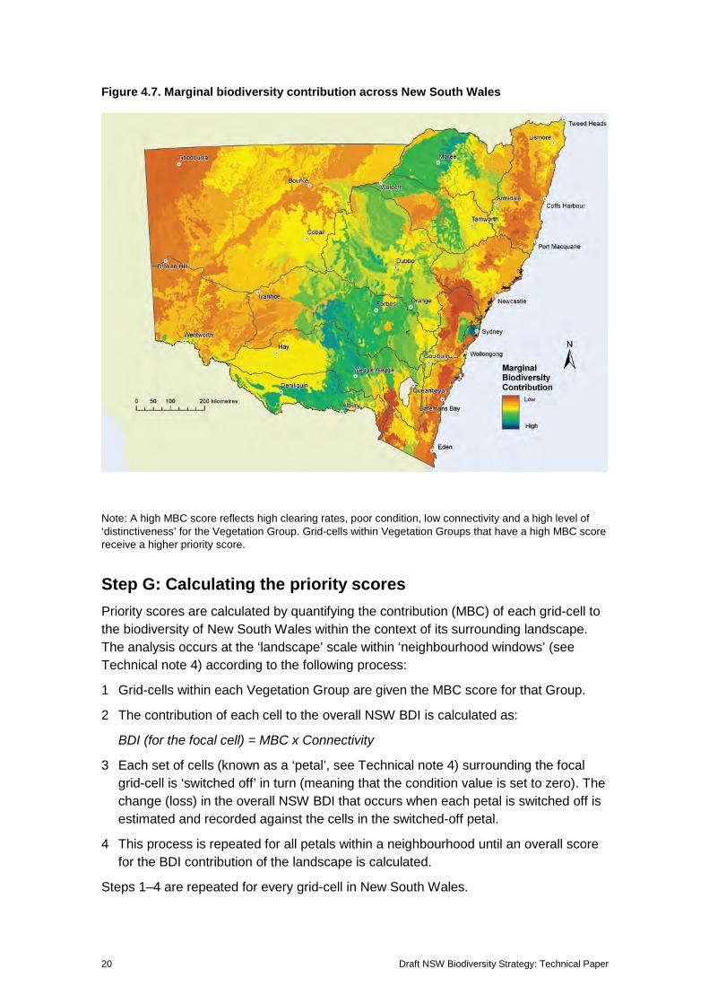
Figure 4.7. Marginal biodiversity contribution across New South Wales
Note: A high MBC score reflects high clearing rates, poor condition, low connectivity and a high level of ‘distinctiveness’ for the Vegetation Group. Grid-cells within Vegetation Groups that have a high MBC score receive a higher priority score.
Step G: Calculating the priority scores Priority scores are calculated by quantifying the contribution (MBC) of each grid-cell to the biodiversity of New South Wales within the context of its surrounding landscape. The analysis occurs at the ‘landscape’ scale within ‘neighbourhood windows’ (see Technical note 4) according to the following process:
1 Grid-cells within each Vegetation Group are given the MBC score for that Group.
2 The contribution of each cell to the overall NSW BDI is calculated as:
BDI (for the focal cell) = MBC x Connectivity
3 Each set of cells (known as a ‘petal’, see Technical note 4) surrounding the focal grid-cell is ‘switched off’ in turn (meaning that the condition value is set to zero). The change (loss) in the overall NSW BDI that occurs when each petal is switched off is estimated and recorded against the cells in the switched-off petal.
4 This process is repeated for all petals within a neighbourhood until an overall score for the BDI contribution of the landscape is calculated.
Steps 1–4 are repeated for every grid-cell in New South Wales.
Deriving Priority Areas for Investment 21
In this way, the overall biodiversity status of the landscape in which each grid-cell is embedded can be assessed, and its contribution to the biodiversity of New South Wales quantified (the NSW BDI score). Through this process, grid-cells that would incur the greatest cost to the biodiversity status of New South Wales (NSW BDI), if they were to be removed, are given the highest priority scores.
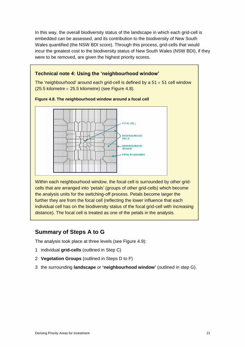
Technical note 4: Using the ‘neighbourhood window’
The ‘neighbourhood’ around each grid-cell is defined by a 51 × 51 cell window (25.5 kilometre × 25.5 kilometre) (see Figure 4.8).
Figure 4.8. The neighbourhood window around a focal cell
Within each neighbourhood window, the focal cell is surrounded by other grid-cells that are arranged into ‘petals’ (groups of other grid-cells) which become the analysis units for the switching-off process. Petals become larger the further they are from the focal cell (reflecting the lower influence that each individual cell has on the biodiversity status of the focal grid-cell with increasing distance). The focal cell is treated as one of the petals in the analysis.
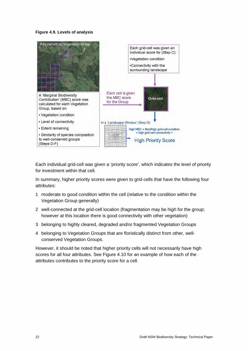
Summary of Steps A to G The analysis took place at three levels (see Figure 4.9):
1 individual grid-cells (outlined in Step C)
2 Vegetation Groups (outlined in Steps D to F)
3 the surrounding landscape or ‘neighbourhood window’ (outlined in step G).
22 Draft NSW Biodiversity Strategy: Technical Paper
Figure 4.9. Levels of analysis
Each individual grid-cell was given a ‘priority score’, which indicates the level of priority for investment within that cell.
In summary, higher priority scores were given to grid-cells that have the following four attributes:
1 moderate to good condition within the cell (relative to the condition within the Vegetation Group generally)
2 well-connected at the grid-cell location (fragmentation may be high for the group; however at this location there is good connectivity with other vegetation)
3 belonging to highly cleared, degraded and/or fragmented Vegetation Groups
4 belonging to Vegetation Groups that are floristically distinct from other, well-conserved Vegetation Groups.
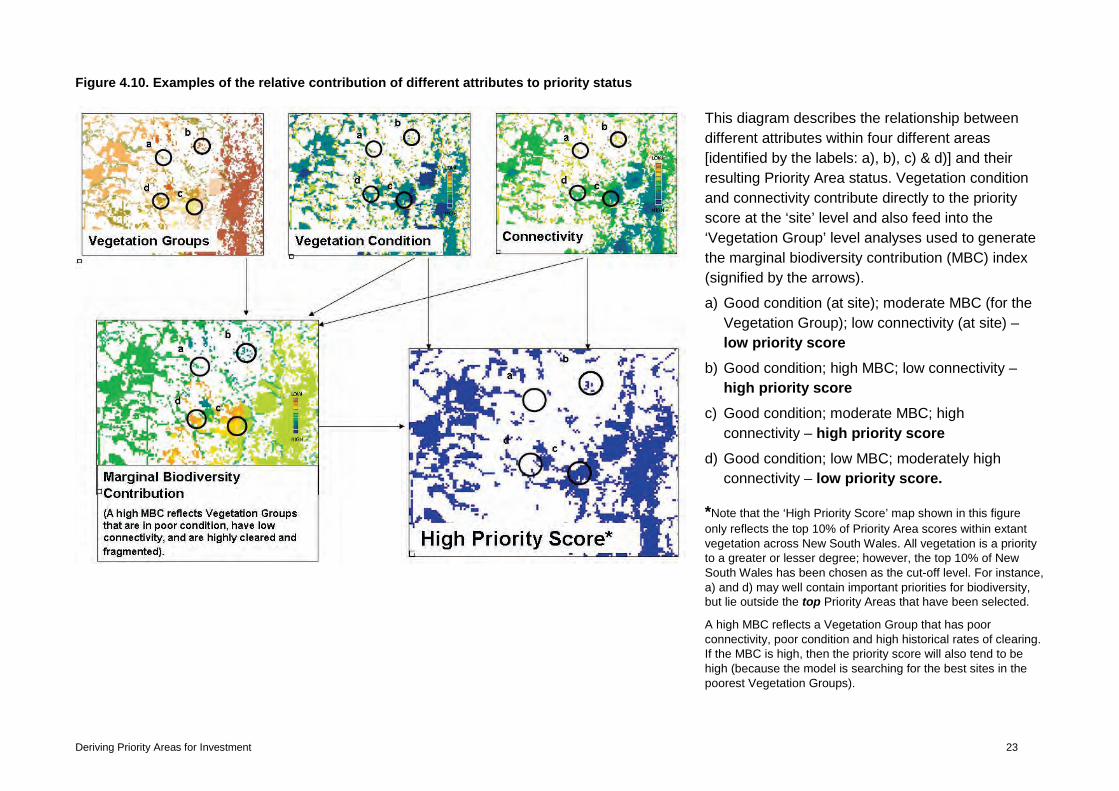
However, it should be noted that higher priority cells will not necessarily have high scores for all four attributes. See Figure 4.10 for an example of how each of the attributes contributes to the priority score for a cell.
Deriving Priority Areas for Investment 23
Figure 4.10. Examples of the relative contribution of different attributes to priority status
This diagram describes the relationship between different attributes within four different areas [identified by the labels: a), b), c) & d)] and their resulting Priority Area status. Vegetation condition and connectivity contribute directly to the priority score at the ‘site’ level and also feed into the ‘Vegetation Group’ level analyses used to generate the marginal biodiversity contribution (MBC) index (signified by the arrows).
a) Good condition (at site); moderate MBC (for the Vegetation Group); low connectivity (at site) – low priority score
b) Good condition; high MBC; low connectivity – high priority score
c) Good condition; moderate MBC; high connectivity – high priority score
d) Good condition; low MBC; moderately high connectivity – low priority score.
*Note that the ‘High Priority Score’ map shown in this figure only reflects the top 10% of Priority Area scores within extant vegetation across New South Wales. All vegetation is a priority to a greater or lesser degree; however, the top 10% of New South Wales has been chosen as the cut-off level. For instance, a) and d) may well contain important priorities for biodiversity, but lie outside the top Priority Areas that have been selected.
A high MBC reflects a Vegetation Group that has poor connectivity, poor condition and high historical rates of clearing. If the MBC is high, then the priority score will also tend to be high (because the model is searching for the best sites in the poorest Vegetation Groups).
24 Draft NSW Biodiversity Strategy: Technical Paper
A real example of priority status
The Upper Castlereagh channels and floodplains between Goonoo and Coolbaggie Nature Reserve have a high priority score. Although the condition of this vegetation is not high, it has been identified as a high priority for investment. The reasons for this are:
1 It most likely contains a native understorey or herb layer with some tree removal.
2 The vegetation in that area is relatively over-cleared, degraded and/or fragmented across its pre-European extent.
3 The area is in close proximity to large patches of intact native vegetation (good connectivity).
Deriving Priority Areas for Investment 25
5 Creating the initial map showing relative priorities
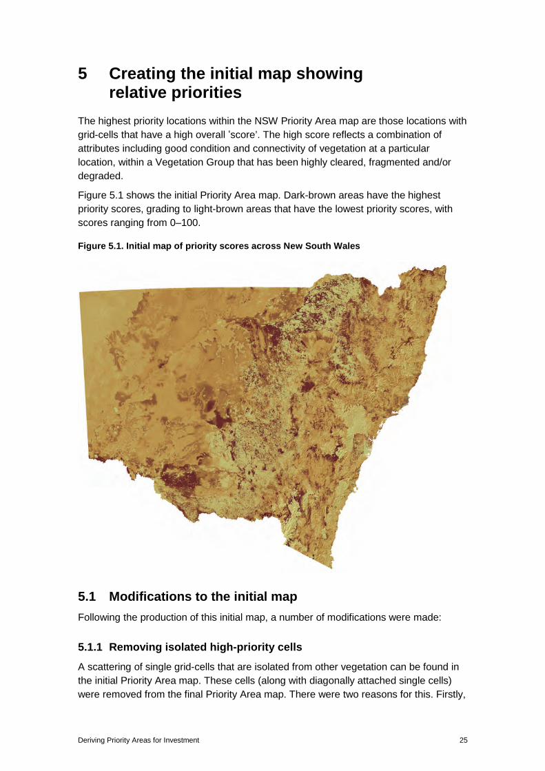
The highest priority locations within the NSW Priority Area map are those locations with grid-cells that have a high overall ‛score’. The high score reflects a combination of attributes including good condition and connectivity of vegetation at a particular location, within a Vegetation Group that has been highly cleared, fragmented and/or degraded.
Figure 5.1 shows the initial Priority Area map. Dark-brown areas have the highest priority scores, grading to light-brown areas that have the lowest priority scores, with scores ranging from 0–100.
Figure 5.1. Initial map of priority scores across New South Wales
5.1 Modifications to the initial map Following the production of this initial map, a number of modifications were made:
5.1.1 Removing isolated high-priority cells
A scattering of single grid-cells that are isolated from other vegetation can be found in the initial Priority Area map. These cells (along with diagonally attached single cells) were removed from the final Priority Area map. There were two reasons for this. Firstly,
26 Draft NSW Biodiversity Strategy: Technical Paper
these cells were removed because they represent remnants of vegetation that are less than 25 hectares in size and are therefore not considered a high priority for investment. Secondly, there is a high degree of error among these single cells, remembering the difficulties of matching individual grid-cells to vegetation ‘on the ground’ at the scale of the map (see Figure 4.1). Viewing these single cells could cause confusion, so they were removed.
5.1.2 Removing high-priority cells from growth centres
The metropolitan and regional strategies developed by the NSW Department of Planning have been used to identify areas known as ‘growth centres’, where new development will be focused to meet the needs of expanding populations. A small proportion of high-priority cells occur in these growth centres. As these areas will be developed it is not appropriate to identify them as high priority for investment in native vegetation and these cells were removed, except for parts of the North West and South West Growth Centres in Western Sydney where native vegetation is to be retained and restored.
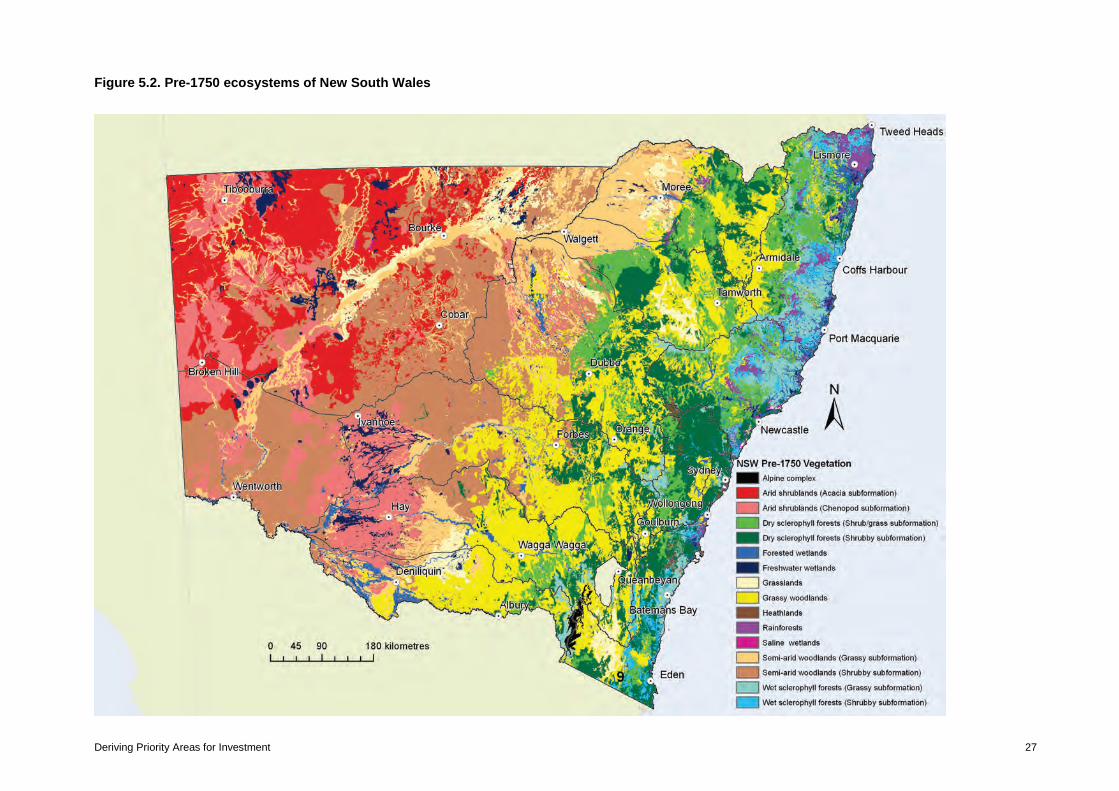
5.2 Ecosystems excluded from the Priority Area map In 2010, DECCW produced a map of the current and modelled pre-1750 distribution of the State’s 12 vegetation formations (hereafter referred to as ‘ecosystems’; Keith and Simpson 2010; see Figure 5.2). These ecosystems are recognisable to most Australians and have been mapped across New South Wales.
The initial map of Priority Areas (Figure 5.1) was intersected with the pre-1750 ecosystems map (Figure 5.2). This allowed the identification of ecosystem types for all Priority Areas.
Deriving Priority Areas for Investment 27
Figure 5.2. Pre-1750 ecosystems of New South Wales
28 Draft NSW Biodiversity Strategy: Technical Paper
A DECCW expert panel reviewed the distribution of the mapped biodiversity Priority Areas for each ecosystem. The panel was made up of DECCW staff with extensive ‘on-ground’ familiarity with the native vegetation of New South Wales. The group decided that the biodiversity priorities map could not be applied to the following three ecosystems for the reasons included.
• Freshwater Wetlands – Vegetation extent and condition has not been mapped adequately in these ecosystems and they cannot be modelled to identify Priority Areas. A set of Freshwater Wetland priorities (including the Macquarie Marshes and the Gwydir Wetlands) have been established, based on existing wetland program priorities and expert opinion. These areas are not indicated on the Priority Area map. Instead, a map showing the location of these important wetlands is included in Part B of the Draft Strategy.
• Arid Shrubland ecosystems – Priorities could not be mapped for the Arid Shrublands of New South Wales for two reasons. Firstly, data on vegetation condition in the Western Division is relatively coarse. Secondly, degradation of Arid Shrublands occurs mostly as a result of total grazing pressure, which is difficult to capture in mapping (compared to ‘clearing’ of woody vegetation, which is easier to identify via satellite imagery). This has made these Arid Shrubland ecosystems difficult to model using the standard BFT approach. Instead, an estimated 10% of the Arid Shrublands has been given priority status for investment, wherever vegetation would significantly benefit from reduced total grazing pressure. These Priority Areas have largely already been identified across much of their range in the Western Catchment Management Area as part of the Western CMA’s Enterprise Based Conservation program. Some particular Priority Areas for Arid Shrublands were identified by an expert panel with local knowledge and these are presented in the Draft Strategy.
• Dry Sclerophyll and Semi-arid Woodland Shrubby subformations – A large area of these subformations was identified on the Priority Area map. Given the large amount of floristic variation across the range of these ecosystems, it is likely that they were assigned a high level of ‘distinctiveness’ compared with other ecosystems. This is likely to have been a key driver of the high-priority status of these ecosystems, at the expense of the core criteria: connectivity, condition and clearing level. The expert panel recommended that they be removed from the Priority Area map because the Grassy subformations are usually of a much higher priority than the Shrubby subformations, given higher past rates of clearing and degradation, lower rates of reservation, and greater likely future land-use pressures.
Freshwater Wetlands, Saline Wetlands and the two Arid Shrubland ecosystems cover approximately 22% of New South Wales. Therefore, 22% of the State was masked from the statewide map because existing information was not suitable for mapping Priority Areas. In contrast, although information is suitable for identifying Priority Areas for Shrubby subformations, the Dry Sclerophyll and Semi-arid Woodland Shrubby subformations, which cover approximately 28% of the State, were masked because these subformations were not considered to be a priority by the expert panel.
Deriving Priority Areas for Investment 29
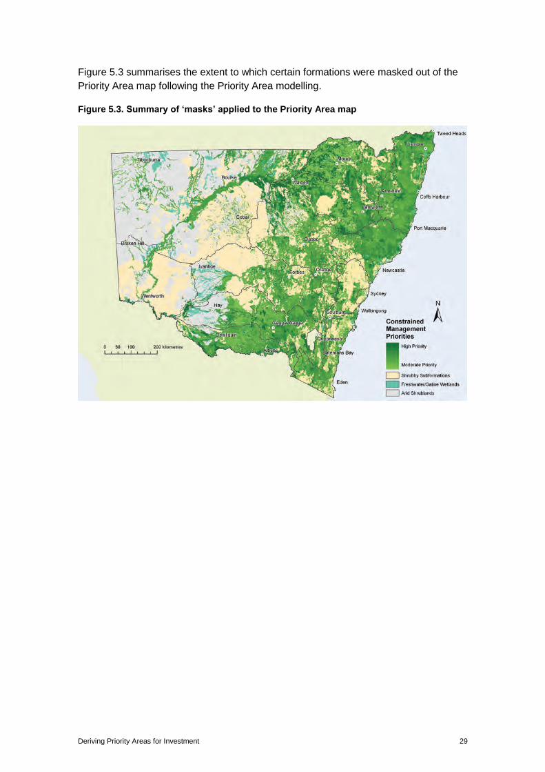
Figure 5.3 summarises the extent to which certain formations were masked out of the Priority Area map following the Priority Area modelling.
Figure 5.3. Summary of ‘masks’ applied to the Priority Area map
30 Draft NSW Biodiversity Strategy: Technical Paper
6 The final Priority Area map A range of potential ‘cut-off’ points were considered when choosing the proportion of extant vegetation to receive priority status. Grid-cells with the top 8.5% of scores (representing 10% of extant native vegetation and 6% of New South Wales as a whole) provided a reasonable balance between identifying a relatively large area, to allow some flexibility for directing investment programs, while still focusing on areas with the greatest potential to contribute to the maintenance and enhancement of biodiversity at a state scale.
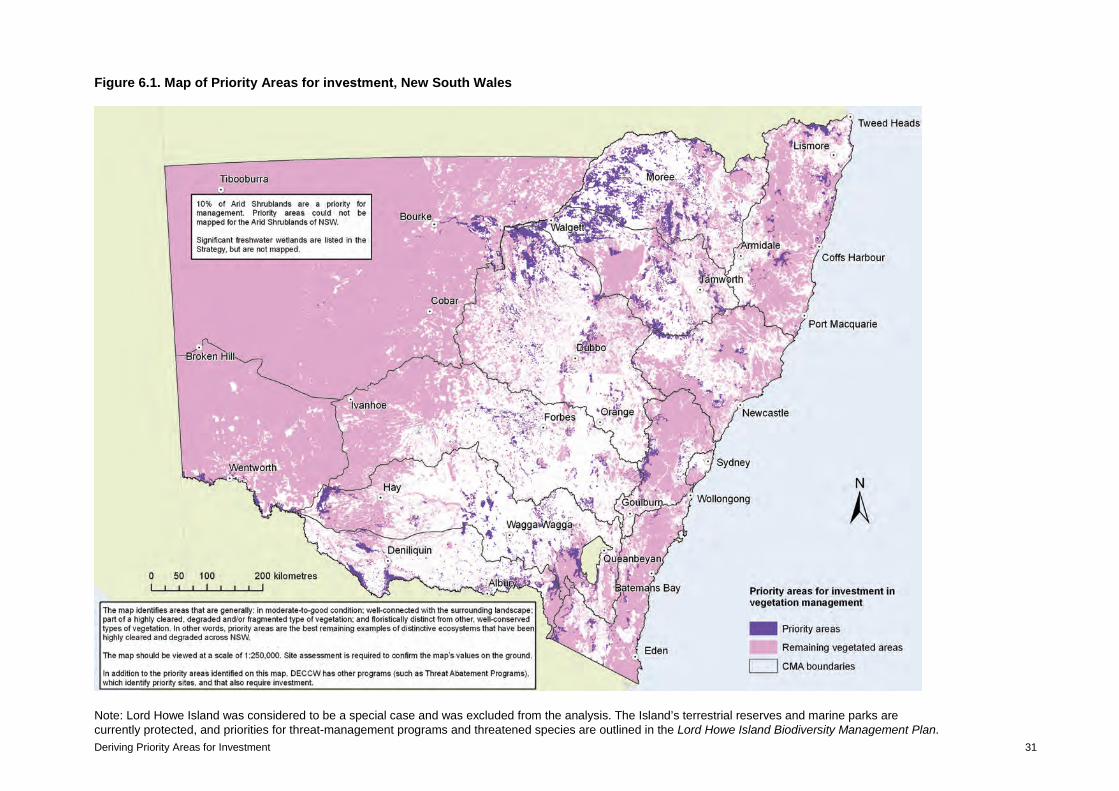
The final Priority Area map is shown below in Figure 6.1. The areas in pink represent extant native vegetation and the areas in purple represent ‘Priority Areas for investment in vegetation management’. This final map is presented as Map 1 in Part A of the Draft Strategy.
The map identifies the best remaining examples of vegetation that are part of highly cleared, degraded and/or fragmented Vegetation Groups. These Priority Areas are generally well-connected and in moderate to good condition. Priority Areas are those areas that are likely to benefit most from investment in management, and where management success is most likely.
The Priority Areas cover approximately 6% of the total area of New South Wales. Two-thirds of the Priority Areas (4% of New South Wales, covering 3.2 million hectares) have been mapped (Figure 6.1), and the remaining one-third (2% of New South Wales, covering 1.6 million hectares) represents Arid Shrubland Priority Areas which could not be mapped.
Deriving Priority Areas for Investment 31
Figure 6.1. Map of Priority Areas for investment, New South Wales
Note: Lord Howe Island was considered to be a special case and was excluded from the analysis. The Island’s terrestrial reserves and marine parks are currently protected, and priorities for threat-management programs and threatened species are outlined in the Lord Howe Island Biodiversity Management Plan.
32 Draft NSW Biodiversity Strategy: Technical Paper
6.1 Viewing the map The map should be viewed at a scale of 1:250,000. Within each 25-hectare (500 metre × 500 metre) grid-cell there is usually a good deal of variation in the vegetation type and structure (see Figure 4.1 for an explanation).
Given the coarse scale of the map, Priority Areas marked are indicative only and site assessment is necessary to confirm Priority Area attributes of sites ‘on the ground’.
Some areas that are classified as ‘cleared’ by Keith (2010) have been identified as Priority Areas on the Priority Area map. These sites may be (i) cleared but incorrectly identified as a Priority Area or (ii) a genuine Priority Area but incorrectly identified as ‘cleared’ by Keith (2010). In reality, given that the mapping is carried out at a coarse scale over a large and complex landscape, both these types of error occur in the priority layer. If Keith’s ‘cleared’ areas were removed from the map, then large areas of genuine priority vegetation would also be removed. If the ‘cleared’ areas were retained, then error will occur because a small proportion of sites that are cleared will appear as Priority Areas on the map. Given that there is error in leaving in or masking out the ‘cleared’ areas, it was decided that the cleared areas should remain, using the rationale that it is better not to exclude potential Priority Areas than it is to include a small proportion of Priority Areas that are actually cleared ‘on the ground’. Therefore, when viewing the map it is important to remember that some grid-cells that have been identified as a priority may be cleared or cropped. Thus, it is essential that site assessment is carried out to verify values on the ground before any investment occurs. Error is highest in more complex landscapes, such as the Darling Riverine Plain, which contains a large number of non-woody ecosystems and a range of land uses that makes interpretation of satellite imagery difficult.
Deriving Priority Areas for Investment 33
7 Relating the Priority Areas to the ecosystems of New South Wales
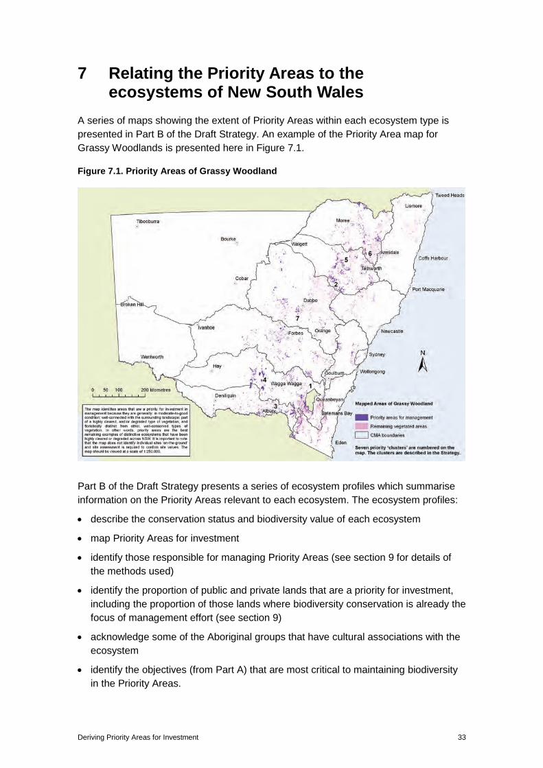
A series of maps showing the extent of Priority Areas within each ecosystem type is presented in Part B of the Draft Strategy. An example of the Priority Area map for Grassy Woodlands is presented here in Figure 7.1.
Figure 7.1. Priority Areas of Grassy Woodland
Part B of the Draft Strategy presents a series of ecosystem profiles which summarise information on the Priority Areas relevant to each ecosystem. The ecosystem profiles:
• describe the conservation status and biodiversity value of each ecosystem
• map Priority Areas for investment
• identify those responsible for managing Priority Areas (see section 9 for details of the methods used)
• identify the proportion of public and private lands that are a priority for investment, including the proportion of those lands where biodiversity conservation is already the focus of management effort (see section 9)
• acknowledge some of the Aboriginal groups that have cultural associations with the ecosystem
• identify the objectives (from Part A) that are most critical to maintaining biodiversity in the Priority Areas.
34 Draft NSW Biodiversity Strategy: Technical Paper
Information on the average level of fragmentation of each ecosystem type is also included in the profiles. Some ecosystem types, such as Dry Sclerophyll Forests are generally distributed within much larger remnants than others, such as Grassy Woodlands. This should be taken into account when deciding whether an area is a Priority Area. For instance, a smaller Grassy Woodland remnant may represent a good investment where a Dry Sclerophyll Forest remnant of the same size may not. See Appendix 3 for a description of the methods used to calculate these figures.
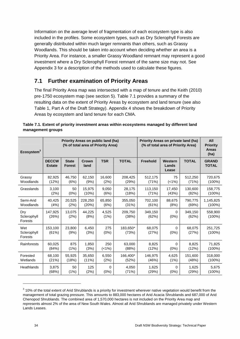
7.1 Further examination of Priority Areas The final Priority Area map was intersected with a map of tenure and the Keith (2010) pre-1750 ecosystem map (see section 5). Table 7.1 provides a summary of the resulting data on the extent of Priority Areas by ecosystem and land tenure (see also Table 1, Part A of the Draft Strategy). Appendix 4 shows the breakdown of Priority Areas by ecosystem and land tenure for each CMA.
Table 7.1. Extent of priority investment areas within ecosystems managed by different land management groups
Ecosystem3
Priority Areas on public land (ha) (% of total area of Priority Area)
Priority Areas on private land (ha) (% of total area of Priority Area)
All Priority Areas (ha)
DECCW Estate
State Forest
Crown land
TSR TOTAL Freehold Western Lands Lease
TOTAL GRAND TOTAL
Grassy Woodlands
82,925 (12%)
46,750 (6%)
62,150 (9%)
16,600 (2%)
208,425 (29%)
512,175 (71%)
75 (<1%)
512,250 (71%)
720,675 (100%)
Grasslands 3,100 (2%)
50 (0%)
15,975 (10%)
9,050 (6%)
28,175 (18%)
113,150 (71%)
17,450 (43%)
130,600 (82%)
158,775 (100%)
Semi-Arid Woodlands
40,425 (4%)
20,525 (2%)
228,250 (20%)
65,850 (6%)
355,050 (31%)
702,100 (61%)
88,675 (8%)
790,775 (69%)
1,145,825 (100%)
Dry Sclerophyll Forests
147,925 (26%)
13,075 (2%)
44,225 (8%)
4,525 (1%)
209,750 (38%)
349,150 (62%)
0 (0%)
349,150 (62%)
558,900 (100%)
Wet Sclerophyll Forests
153,100 (61%)
23,800 (9%)
6,450 (3%)
275 (0%)
183,650* (73%)
68,075 (27%)
0 (0%)
68,075 (27%)
251,725 (100%)
Rainforests 60,025 (84%)
875 (1%)
1,850 (3%)
250 (<1%)
63,000 (88%)
8,825 (12%)
0 (0%)
8,825 (12%)
71,825 (100%)
Forested Wetlands
68,100 (21%)
55,925 (18%)
35,650 (11%)
6,550 (2%)
166,400* (52%)
146,975 (46%)
4,625 (1%)
151,600 (48%)
318,000 (100%)
Heathlands 3,875 (68%)
50 (1%)
125 (2%)
0 (0%)
4,050 (71%)
1,625 (29%)
0 (0%)
1,625 (29%)
5,675 (100%)
3 10% of the total extent of Arid Shrublands is a priority for investment wherever native vegetation would benefit from the management of total grazing pressure. This amounts to 883,000 hectares of Arid Acacia Shrublands and 687,000 of Arid Chenopod Shrublands. The combined area of 1,570,000 hectares is not included on the Priority Area map and represents almost 2% of the area of New South Wales. Almost all Arid Shrublands are managed privately under Western Lands Leases.
Deriving Priority Areas for Investment 35
Ecosystem3
Priority Areas on public land (ha) (% of total area of Priority Area)
Priority Areas on private land (ha) (% of total area of Priority Area)
All Priority Areas (ha)
DECCW Estate
State Forest
Crown land
TSR TOTAL Freehold Western Lands Lease
TOTAL GRAND TOTAL
Alpine Complex
6,850 (100%)
0 (0%)
0 (0%)
0 (0%)
6,850 (100%)
25 (0%)
0 (0%)
25 (<1%)
6,875 (100%)
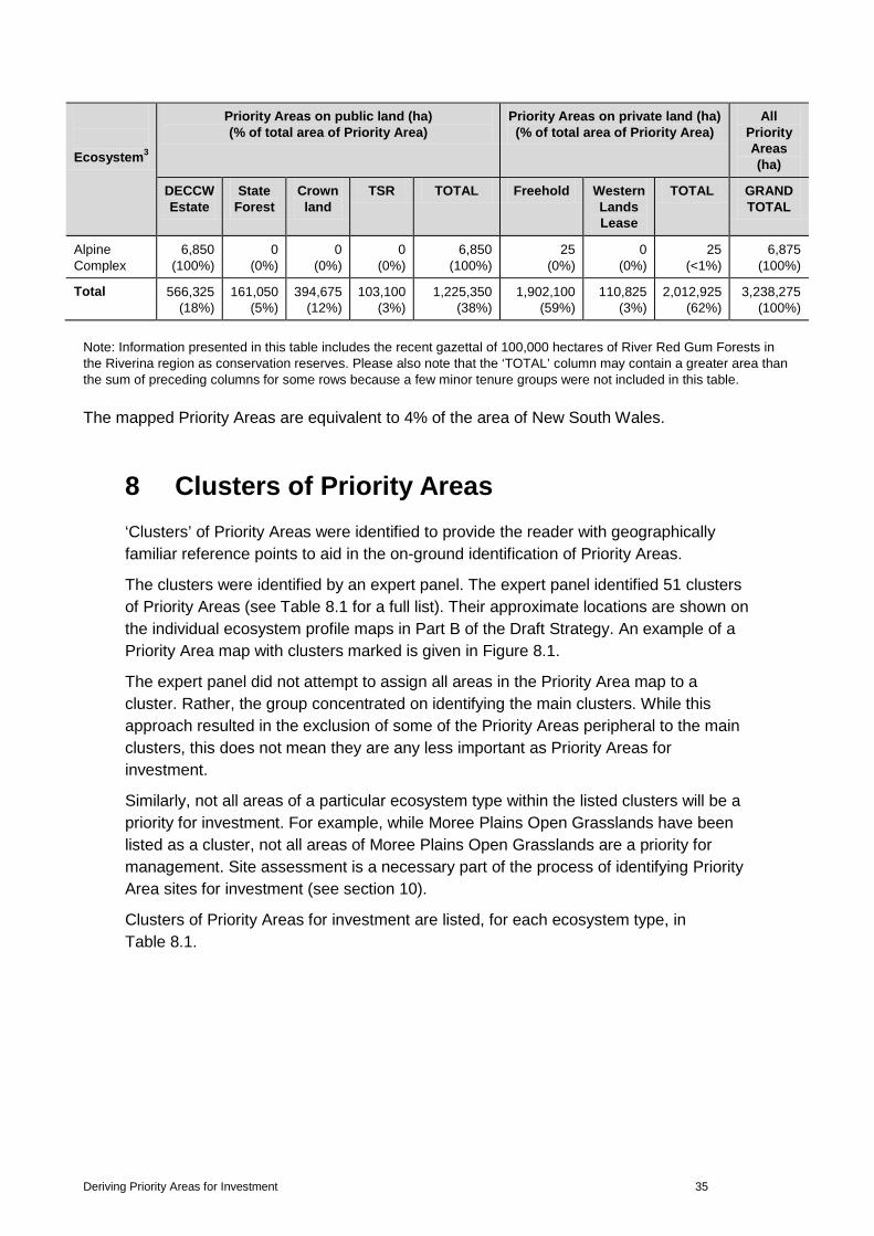
Total 566,325 (18%)
161,050 (5%)
394,675 (12%)
103,100 (3%)
1,225,350 (38%)
1,902,100 (59%)
110,825 (3%)
2,012,925 (62%)
3,238,275 (100%)
Note: Information presented in this table includes the recent gazettal of 100,000 hectares of River Red Gum Forests in the Riverina region as conservation reserves. Please also note that the ‘TOTAL’ column may contain a greater area than the sum of preceding columns for some rows because a few minor tenure groups were not included in this table.
The mapped Priority Areas are equivalent to 4% of the area of New South Wales.
8 Clusters of Priority Areas ‘Clusters’ of Priority Areas were identified to provide the reader with geographically familiar reference points to aid in the on-ground identification of Priority Areas.
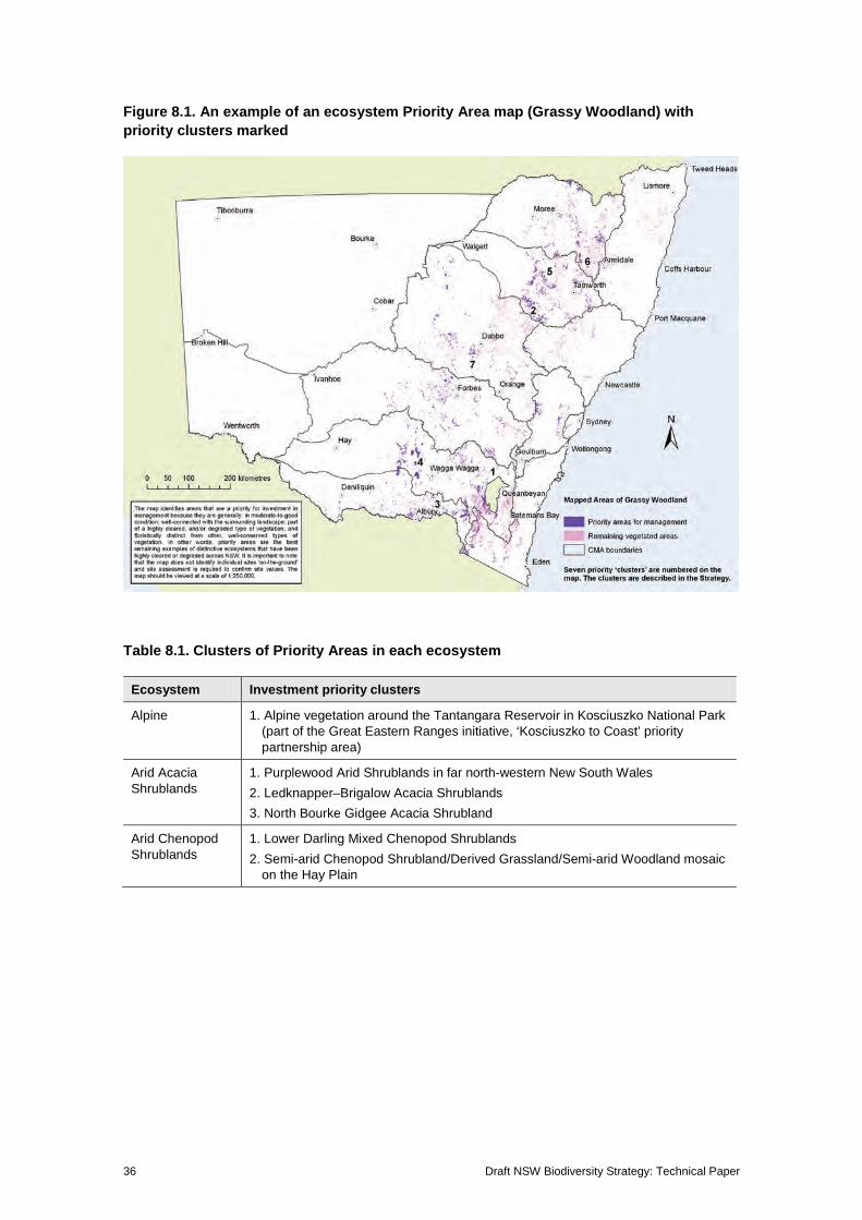
The clusters were identified by an expert panel. The expert panel identified 51 clusters of Priority Areas (see Table 8.1 for a full list). Their approximate locations are shown on the individual ecosystem profile maps in Part B of the Draft Strategy. An example of a Priority Area map with clusters marked is given in Figure 8.1.
The expert panel did not attempt to assign all areas in the Priority Area map to a cluster. Rather, the group concentrated on identifying the main clusters. While this approach resulted in the exclusion of some of the Priority Areas peripheral to the main clusters, this does not mean they are any less important as Priority Areas for investment.
Similarly, not all areas of a particular ecosystem type within the listed clusters will be a priority for investment. For example, while Moree Plains Open Grasslands have been listed as a cluster, not all areas of Moree Plains Open Grasslands are a priority for management. Site assessment is a necessary part of the process of identifying Priority Area sites for investment (see section 10).
Clusters of Priority Areas for investment are listed, for each ecosystem type, in Table 8.1.
36 Draft NSW Biodiversity Strategy: Technical Paper
Figure 8.1. An example of an ecosystem Priority Area map (Grassy Woodland) with priority clusters marked
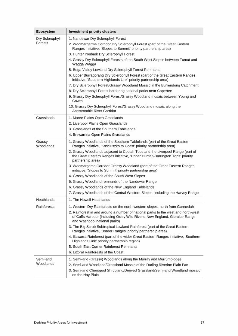
Table 8.1. Clusters of Priority Areas in each ecosystem
Ecosystem Investment priority clusters
Alpine 1. Alpine vegetation around the Tantangara Reservoir in Kosciuszko National Park (part of the Great Eastern Ranges initiative, ‘Kosciuszko to Coast’ priority partnership area)
Arid Acacia Shrublands
1. Purplewood Arid Shrublands in far north-western New South Wales 2. Ledknapper–Brigalow Acacia Shrublands 3. North Bourke Gidgee Acacia Shrubland
Arid Chenopod Shrublands
1. Lower Darling Mixed Chenopod Shrublands 2. Semi-arid Chenopod Shrubland/Derived Grassland/Semi-arid Woodland mosaic
on the Hay Plain
Deriving Priority Areas for Investment 37
Ecosystem Investment priority clusters
Dry Sclerophyll Forests
1. Nandewar Dry Sclerophyll Forest 2. Woomargarma Corridor Dry Sclerophyll Forest (part of the Great Eastern
Ranges initiative, ‘Slopes to Summit’ priority partnership area) 3. Hunter Ironbark Dry Sclerophyll Forest 4. Grassy Dry Sclerophyll Forests of the South West Slopes between Tumut and
Wagga Wagga 5. Bega Valley Lowland Dry Sclerophyll Forest Remnants 6. Upper Burragorang Dry Sclerophyll Forest (part of the Great Eastern Ranges
initiative, ‘Southern Highlands Link’ priority partnership area) 7. Dry Sclerophyll Forest/Grassy Woodland Mosaic in the Burrendong Catchment 8. Dry Sclerophyll Forest bordering national parks near Capertee 9. Grassy Dry Sclerophyll Forest/Grassy Woodland mosaic between Young and
Cowra 10. Grassy Dry Sclerophyll Forest/Grassy Woodland mosaic along the
Abercrombie River Corridor
Grasslands 1. Moree Plains Open Grasslands 2. Liverpool Plains Open Grasslands 3. Grasslands of the Southern Tablelands 4. Brewarrina Open Plains Grasslands
Grassy Woodlands
1. Grassy Woodlands of the Southern Tablelands (part of the Great Eastern Ranges initiative, ‘Kosciuszko to Coast’ priority partnership area)
2. Grassy Woodlands adjacent to Coolah Tops and the Liverpool Range (part of the Great Eastern Ranges initiative, ‘Upper Hunter–Barrington Tops’ priority partnership area)
3. Woomargama Corridor Grassy Woodland (part of the Great Eastern Ranges initiative, ‘Slopes to Summit’ priority partnership area)
4. Grassy Woodlands of the South West Slopes 5. Grassy Woodland remnants of the Nandewar Range 6. Grassy Woodlands of the New England Tablelands 7. Grassy Woodlands of the Central Western Slopes, including the Harvey Range
Heathlands 1. The Howell Heathlands
Rainforests 1. Western Dry Rainforests on the north-western slopes, north from Gunnedah 2. Rainforest in and around a number of national parks to the west and north-west
of Coffs Harbour (including Oxley Wild Rivers, New England, Gibraltar Range and Washpool national parks)
3. The Big Scrub Subtropical Lowland Rainforest (part of the Great Eastern Ranges initiative, ‘Border Ranges’ priority partnership area)
4. Illawarra Rainforest (part of the wider Great Eastern Ranges initiative, ‘Southern Highlands Link’ priority partnership region)
5. South East Corner Rainforest Remnants 6. Littoral Rainforests of the Coast
Semi-arid Woodlands
1. Semi-arid (Grassy) Woodlands along the Murray and Murrumbidgee 2. Semi-arid Woodland/Grassland Mosaic of the Darling Riverine Plain Fan 3. Semi-arid Chenopod Shrubland/Derived Grassland/Semi-arid Woodland mosaic
on the Hay Plain
38 Draft NSW Biodiversity Strategy: Technical Paper
Ecosystem Investment priority clusters
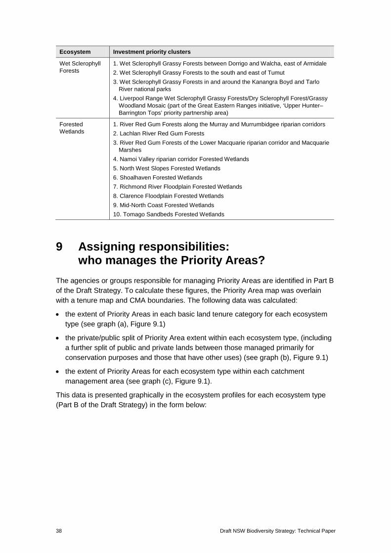
Wet Sclerophyll Forests
1. Wet Sclerophyll Grassy Forests between Dorrigo and Walcha, east of Armidale 2. Wet Sclerophyll Grassy Forests to the south and east of Tumut 3. Wet Sclerophyll Grassy Forests in and around the Kanangra Boyd and Tarlo
River national parks 4. Liverpool Range Wet Sclerophyll Grassy Forests/Dry Sclerophyll Forest/Grassy
Woodland Mosaic (part of the Great Eastern Ranges initiative, ‘Upper Hunter–Barrington Tops’ priority partnership area)
Forested Wetlands
1. River Red Gum Forests along the Murray and Murrumbidgee riparian corridors 2. Lachlan River Red Gum Forests 3. River Red Gum Forests of the Lower Macquarie riparian corridor and Macquarie
Marshes 4. Namoi Valley riparian corridor Forested Wetlands 5. North West Slopes Forested Wetlands 6. Shoalhaven Forested Wetlands 7. Richmond River Floodplain Forested Wetlands 8. Clarence Floodplain Forested Wetlands 9. Mid-North Coast Forested Wetlands 10. Tomago Sandbeds Forested Wetlands
9 Assigning responsibilities: who manages the Priority Areas?
The agencies or groups responsible for managing Priority Areas are identified in Part B of the Draft Strategy. To calculate these figures, the Priority Area map was overlain with a tenure map and CMA boundaries. The following data was calculated:
• the extent of Priority Areas in each basic land tenure category for each ecosystem type (see graph (a), Figure 9.1)
• the private/public split of Priority Area extent within each ecosystem type, (including a further split of public and private lands between those managed primarily for conservation purposes and those that have other uses) (see graph (b), Figure 9.1)
• the extent of Priority Areas for each ecosystem type within each catchment management area (see graph (c), Figure 9.1).
This data is presented graphically in the ecosystem profiles for each ecosystem type (Part B of the Draft Strategy) in the form below:
Deriving Priority Areas for Investment 39
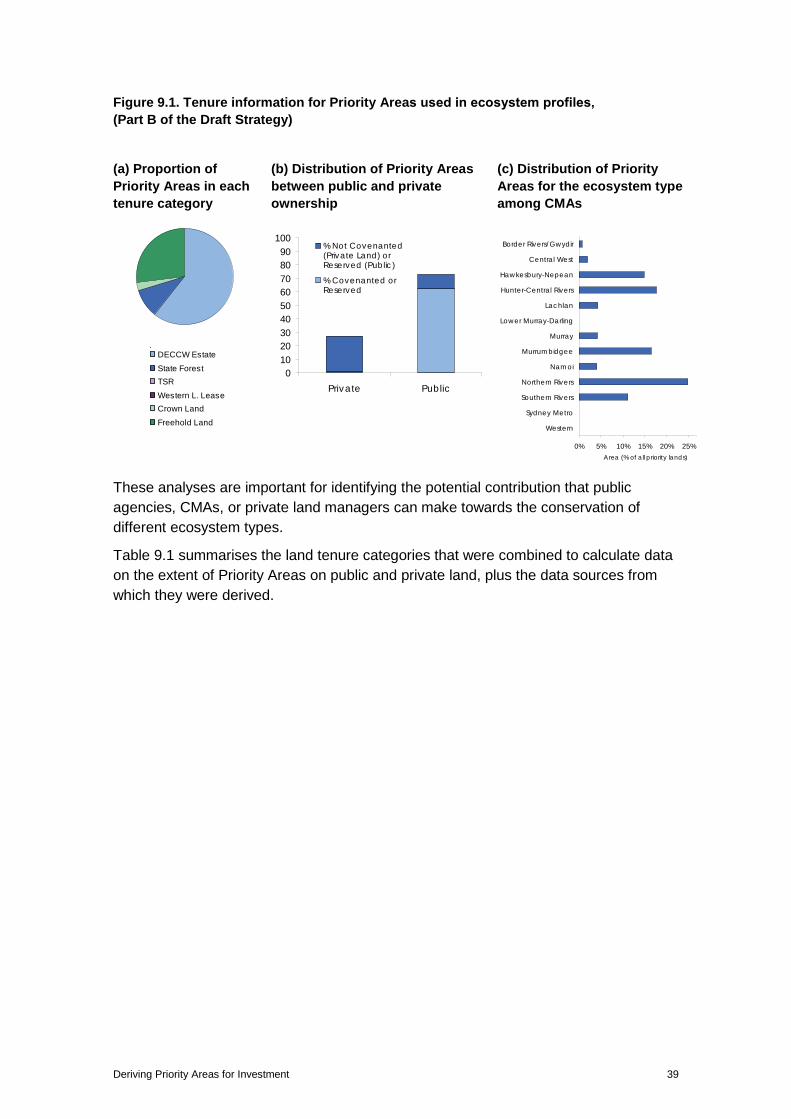
Figure 9.1. Tenure information for Priority Areas used in ecosystem profiles, (Part B of the Draft Strategy)
(a) Proportion of Priority Areas in each tenure category
DECCW Estate
State ForestTSR
Western L. LeaseCrown Land
Freehold Land
(b) Distribution of Priority Areas between public and private ownership
0102030405060708090
100
Private Public
% Not Covenanted(Private Land) orReserved (Public)
% Covenanted orReserved
(c) Distribution of Priority Areas for the ecosystem type among CMAs
0% 5% 10% 15% 20% 25%
Western
Sydney Metro
Southern Rivers
Northern Rivers
Namoi
Murrumbidgee
Murray
Lower Murray-Darling
Lachlan
Hunter-Central Rivers
Hawkesbury-Nepean
Central West
Border Rivers/Gwydir
Area (% of all priority lands)
These analyses are important for identifying the potential contribution that public agencies, CMAs, or private land managers can make towards the conservation of different ecosystem types.
Table 9.1 summarises the land tenure categories that were combined to calculate data on the extent of Priority Areas on public and private land, plus the data sources from which they were derived.
40 Draft NSW Biodiversity Strategy: Technical Paper
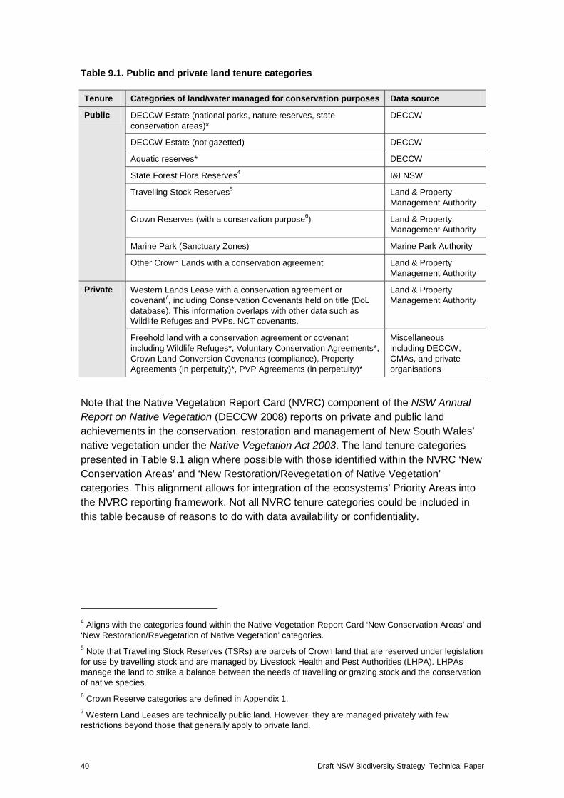
Table 9.1. Public and private land tenure categories
Tenure Categories of land/water managed for conservation purposes Data source
Public DECCW Estate (national parks, nature reserves, state conservation areas)*
DECCW
DECCW Estate (not gazetted) DECCW
Aquatic reserves* DECCW
State Forest Flora Reserves4 I&I NSW
Travelling Stock Reserves5 Land & Property Management Authority
Crown Reserves (with a conservation purpose6) Land & Property Management Authority
Marine Park (Sanctuary Zones) Marine Park Authority
Other Crown Lands with a conservation agreement Land & Property Management Authority
Private Western Lands Lease with a conservation agreement or covenant7, including Conservation Covenants held on title (DoL database). This information overlaps with other data such as Wildlife Refuges and PVPs. NCT covenants.
Land & Property Management Authority
Freehold land with a conservation agreement or covenant including Wildlife Refuges*, Voluntary Conservation Agreements*, Crown Land Conversion Covenants (compliance), Property Agreements (in perpetuity)*, PVP Agreements (in perpetuity)*
Miscellaneous including DECCW, CMAs, and private organisations
Note that the Native Vegetation Report Card (NVRC) component of the NSW Annual Report on Native Vegetation (DECCW 2008) reports on private and public land achievements in the conservation, restoration and management of New South Wales’ native vegetation under the Native Vegetation Act 2003. The land tenure categories presented in Table 9.1 align where possible with those identified within the NVRC ‘New Conservation Areas’ and ‘New Restoration/Revegetation of Native Vegetation’ categories. This alignment allows for integration of the ecosystems’ Priority Areas into the NVRC reporting framework. Not all NVRC tenure categories could be included in this table because of reasons to do with data availability or confidentiality.
4 Aligns with the categories found within the Native Vegetation Report Card ‘New Conservation Areas’ and ‘New Restoration/Revegetation of Native Vegetation’ categories. 5 Note that Travelling Stock Reserves (TSRs) are parcels of Crown land that are reserved under legislation for use by travelling stock and are managed by Livestock Health and Pest Authorities (LHPA). LHPAs manage the land to strike a balance between the needs of travelling or grazing stock and the conservation of native species. 6 Crown Reserve categories are defined in Appendix 1. 7 Western Land Leases are technically public land. However, they are managed privately with few restrictions beyond those that generally apply to private land.
Deriving Priority Areas for Investment 41
10 Using the maps: how to find Priority Areas ‛on the ground’
It is important to remember that the Priority Area map (Figure 6.1, see also Figure 1, Part A of the Draft Strategy) is based on modelling undertaken at a state scale. Site assessment is required to confirm Priority Area status when allocating investment to sites ‘on the ground’.
A site would be considered to be within a Priority Area if it has most of the following attributes:
• good to moderate condition
• well-connected with other vegetation in the surrounding landscape
• part of a type of vegetation that has been highly cleared, degraded and/or fragmented within the region
• within an area identified as a Priority Area or cluster on the Priority Area map
• a particularly distinctive type of vegetation that is not well-conserved in the region
• part of a larger patch-size for that ecosystem (see Appendix 3 for a summary of patch sizes within different ecosystems)
• outside a mapped Priority Area, but satisfying most of the criteria listed above.
In a small number of instances, degraded vegetation may be identified if it scores very high on all other attributes in the BFT model. In addition, there is a small, but measurable level of error in the map, given that it is generated at a state scale. Investment is not appropriate in these cleared or highly degraded areas. Site assessment is essential for locating priority sites for investment, using the Priority Area map as an indicative guide.
Decisions about the particular management actions that are most appropriate at a specific site are best made by individual land managers; supported by CMAs and agency staff.
It should be remembered that different ecosystem types have a different average condition. Decisions about what is a ‘good’ remnant of Grassy Woodland, (which is generally in poor condition and highly fragmented), will be different to a ‘good’ remnant of Dry Sclerophyll Forest. The relative condition of different ecosystem types should be taken into account when deciding whether a site is worthy of investment.
10.1 Should all high Priority Areas be actively managed for biodiversity?
The NSW Priority Area map identifies 6% of terrestrial New South Wales where appropriate investment is expected to yield the greatest improvement to overall biodiversity. This represents a greater area than current resourcing would allow New South Wales to actively manage over the next five years. Therefore not all Priority Areas will be actively managed for biodiversity over the life of the Draft Strategy.
42 Draft NSW Biodiversity Strategy: Technical Paper
Rather, the map provides a range of solid options for agencies, CMAs, landholders and other biodiversity investors to choose from. It also provides a ‘prospectus’ of important areas for investment for funding bodies.
The Priority Area map does not reflect all biodiversity priorities for New South Wales. Priorities for aquatic ecosystems and Arid Shrublands are not mapped but require investment. Some areas (particularly at finer scales) may contain high value biodiversity assets that are currently well-managed for biodiversity, but not identified as Priority Areas. These management programs should continue. Careful consideration should be given before diverting investment from any existing programs, particularly those programs that are achieving success and have a high level of involvement from the community. The Priority Area map presented in this Draft Strategy is static. However, as investment translates into improvements in biodiversity, the priorities will change. The Priority Area map will be updated for the next Biodiversity Strategy to reflect relevant priorities and improved information.
10.2 How should the map be used? The map is designed to be used by both private and public investors to focus investment in priority locations.
CMAs implement a range of native vegetation programs on private and leasehold land, utilising funding from both the NSW and Australian Governments. The Priority Area map identifies key locations that would benefit from CMA investment. The Draft Strategy has set a target of 50% of total CMA investment in native vegetation programs to be spent in Priority Areas.
Deriving Priority Areas for Investment 43
11 References DEC 2006, Decision Support Tools for Biodiversity Conservation: Biodiversity
Forecasting Toolkit, Prepared by DEC for the Comprehensive Coastal Assessment (DoP), Department of Environment and Conservation (NSW), Armidale.
DECCW 2008, NSW Annual Report on Native Vegetation 2008, Department of Environment, Climate Change and Water NSW, Sydney. (http://www.environment.nsw.gov.au/resources/nativeveg/09523arnv08.pdf) Accessed 8/6/2010.
DECCW and Dillon M, McNellie M & Oliver I (in press), Technical Background Report NSW State of the Catchments 2008: Native Vegetation, Scientific Services Division, Department of Environment, Climate Change and Water NSW, Sydney.
Drielsma M J & Ferrier S 2006, ‘Landscape scenario modelling of vegetation condition’, Ecological Management and Restoration, 7: S45–S52.
Drielsma M J, Ferrier S & Manion G 2007, ‘A raster-based technique for analysing habitat configuration: The cost-benefit approach’, Ecological Modelling, 202: 324–332.
Ferrier S 2002, ‘Mapping spatial pattern in biodiversity for regional conservation planning where to from here?’ Systematic Biology, 51: 331–363.
Ferrier S & Drielsma M 2010, ‘Synthesis of pattern and process in biodiversity conservation assessment: a flexible whole-landscape modelling framework’, Diversity and Distributions, 16: 386–402.
Ferrier S, Drielsma M, Manion G & Watson G 2002, ‘Extended statistical approaches to modelling spatial pattern in biodiversity in northeast New South Wales. II. Community-level modelling’, Biodiversity and Conservation, 11: 2309–2338.
Ferrier S, Manion G, Elith J & Richardson K 2007, ‘Using generalized dissimilarity modelling to analyse and predict patterns of beta diversity in regional biodiversity assessment’, Diversity and Distributions, 13: 252–264.
Ferrier S, Powell G V N, Richardson K S, Manion G, Overton J M, Allnutt T F, Cameron S E, Mantle K, Burgess N D, Faith D P, Lamoreux J F, Kier G, Hijmans R J, Funk V A, Cassis G, Fisher B L, Flemons P, Lees D, Lovett J C & Van Rompaey R S A R 2004, ‘Mapping more of terrestrial biodiversity for global conservation assessment’, BioScience, 54: 1101–1109.
Hanski I 1999, ‘Habitat connectivity, habitat continuity, and metapopulations in dynamic landscapes’, Oikos, 87: 209–219.
Harte J, McCarthy S, Taylor K, Kinzig A & Fisher M L 1999, ‘Estimating species-area relationships from plot to landscape scale using spatial-turnover data’, Oikos, 86: 45–54.
Keith D A 2004, Ocean shores to desert dunes, Department of Environment and Conservation (NSW), Hurstville.
Keith D A and Simpson C C 2010, NSW Vegetation Formations (Version 3.0), Report to the NSW Rural Fire Service.
Logan V, Ferrier S & Manion G 2009, ‘Using modelling of continuous gradients of community composition to assess vulnerability of biodiversity to climate change in

44 Draft NSW Biodiversity Strategy: Technical Paper
New South Wales’, Poster presentation at the 10th International Congress of Ecology (INTECOL) 2009 Conference, Brisbane.
Mitchell P B 2002, NSW ecosystems study: background and methodology, Unpublished report to the NSW National Parks and Wildlife Service, Hurstville.
Thackway R & Leslie R 2005, Vegetation, assets, states and transitions: accounting for vegetation condition in the Australian landscape. BRS Technical Report, Bureau of Rural Sciences, Canberra.
Walker P J & Soil Conservation Service of New South Wales 1991, Land systems of western New South Wales, Soil Conservation Service of NSW, Sydney.
Deriving Priority Areas for Investment 45
Appendix 1: Categories of Crown Reserves with a conservation purpose
• Addition~Water Supply
• Camping~Preservation of Water Supply
• Camping~Public Recreation~Water Supply
• Camping~Water Supply
• Catchment Area
• Catchment Area~Soil Conservation
• Coastal Environmental Protection~Public Recreation
• Community Purposes~Environmental Protection
• Community Purposes~Environmental Protection~Heritage Purposes
• Community Purposes~Environmental Protection~Public Recreation
• Conservation of Native Flora~Fauna
• Crossing~Preservation of Native Flora
• Drainage~Environmental Protection~Public Recreation
• Drainage~Preservation of Fauna~Preservation of Native Flora
• Environmental Protection
• Environmental Protection~Future Public Requirements
• Environmental Protection~Future Public Requirements~Public Recreation
• Environmental Protection~Heritage Purposes
• Environmental Protection~Heritage Purposes~Public Recreation
• Environmental Protection~Preservation of Scenery~Public Recreation
• Environmental Protection~Public Recreation
• Environmental Protection~Public Recreation~Rural Services
• Environmental Protection~Public Recreation~Tourist Facilities and Services
• Environmental Protection~Public Recreation~Water
• Environmental Protection~Public Recreation~Water Supply
• Environmental Protection~Rural Services
• Extension~Preservation of Water Supply
• Extension~Water Supply
• Fauna~Preservation of Native Flora
• Future Public Requirements
• Future Public Requirements~Preservation of Fauna~Preservation of Native Flora
• Future Public Requirements~Preservation of Trees
• Heritage Purposes~Public Recreation and Coastal Environmental Protection
• Native Birds~Preservation of Fauna
• Native Fauna~Preservation of Native Flora
• Native Fauna~Preservation of Native Flora~Public Recreation
• Other Public Purposes~Preservation Of Timber~Water Supply
• Other Public Purposes~Preservation of Water Supply
• Other Public Purposes~Water Supply
• Preservation and Growth of Native Flora
• Preservation and Growth of Timber
• Preservation of Aboriginal Carvings and Drawings
• Preservation of Aboriginal Cultural Heritage
• Preservation of Aboriginal Relics~Preservation of Trees
• Preservation of Caves
46 Draft NSW Biodiversity Strategy: Technical Paper
• Preservation of Caves~Preservation of Native Flora and Fauna
• Preservation of Fauna
• Preservation of Fauna~Preservation of Native Flora
• Preservation of Fauna~Preservation of Native Flora~Public Recreation
• Preservation of Fauna~Public Recreation
• Preservation of Native Birds
• Preservation of Native Fauna~Preservation Of Native Flora
• Preservation of Native Fauna~Preservation of Native Flora~Public Recreation
• Preservation of Native Flora And Fauna
• Preservation of Native Flora And Fauna~Preservation Of Timber
• Preservation of Native Flora And Fauna~Preservation Of Trees
• Preservation of Native Flora and Fauna~Public Recreation
• Preservation Of Native Flora and Fauna~Public Recreation~Resting Place
• Preservation of Native Flora~Preservation of Native Flora and Fauna~Public Recreation
• Preservation of Native Flora~Preservation of Scenery
• Preservation of Native Flora~Protection from Sand Drift~Public Recreation
• Preservation of Native Flora~Public Baths~Public Recreation
• Preservation of Native Flora~Public Recreation
• Preservation of Native Flora~Public Recreation~Reservoir
• Preservation of Native Flora~Water Supply
• Preservation of Scenery
• Preservation of Scenery~Public Recreation
• Preservation of Trees~Public Recreation
• Preservation of Trees~Recreation
• Preservation of Trees~Soil Conservation
• Preservation of Water Supply
• Promotion of The Study And Conservation of Native Flora And Fauna
• Promotion of The Study And Preservation of Native Flora
• Promotion of the Study and the Preservation of Native Flora and Fauna
• Promotion of the Study and the Preservation of Native Flora and Fauna~Public Recreation
• Promotion of the Study and the Preservation of Native Flora and Fauna~Public School Purposes
• Protection of Fossil Trees
• Public Purposes~Water Supply
• Public Recreation And Coastal Environmental Protection
• Public Recreation and Coastal Environmental Protection~Tourist Facilities and Services
• Public Recreation and Preservation of Aboriginal Cultural Heritage
• Public Recreation~Water Supply
• Scenic Protection
• Soil Conservation
• Water Supply
Deriving Priority Areas for Investment 47
Appendix 2: Aggregating the BDI values for Vegetation Groups into a single BDI for New South Wales If all Vegetation Groups were considered to have distinct species composition (that is, no species occurring in more than a single Vegetation Group) or if the overarching aim of the analysis was the conservation of groups rather than the species within them, then the Vegetation Group BDI could simply be summed and the possible BDI values would range from 0–572.
In this analysis the compositional overlap was calculated based on a generalised disimilarity model (GDM) of New South Wales.
Generalised Dissimilarity Model (GDM) The Generalised Dissimilarity Model (GDM) (Logan et al. 2009) comprises four environmental surfaces: • AnuClim_01 = mean annual temperature • AnuClim_05 = max. temperature for warmest period • AnuClim_01 = mean annual precipitation • AnuClim_01 = max. precipitation for driest quarter.
The values of each surface have been transformed with a non-linear transformation such that the transformed values represent a linear relationship between the variable and species turnover. The steps are as follows:
1 A set of sites were selected within each geomorphological unit. Where available, the original YETI plot sites were selected. Where insufficient or no YETI sites were available within a unit, sites were randomly generated for that unit.
2 The average dissimilarity between every pair of groups was calculated (using the Bray-Curtis distance measure) based on the GDM environmental attributes at the sites. This resulted in a unit-by-unit dissimilarity matrix.
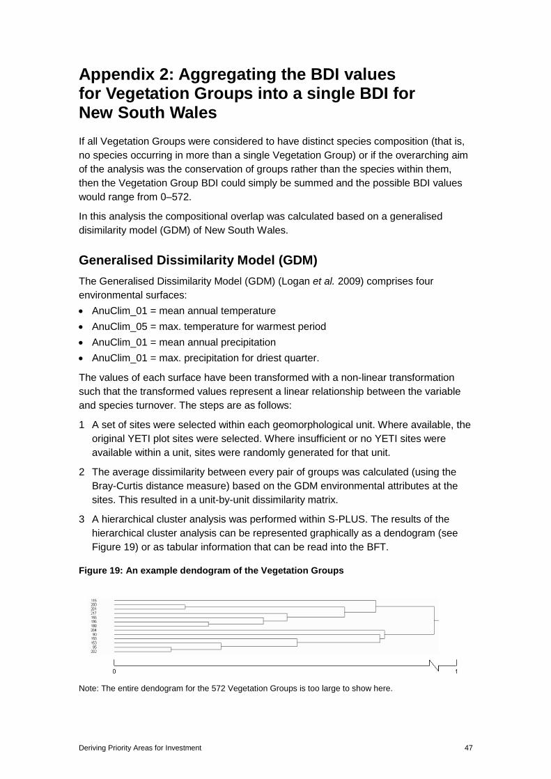
3 A hierarchical cluster analysis was performed within S-PLUS. The results of the hierarchical cluster analysis can be represented graphically as a dendogram (see Figure 19) or as tabular information that can be read into the BFT.
Figure 19: An example dendogram of the Vegetation Groups
Note: The entire dendogram for the 572 Vegetation Groups is too large to show here.
48 Draft NSW Biodiversity Strategy: Technical Paper
The dendogram represents how the groups relate in a hierarchical structure. The horizontal axis represents the biological distance, measured using the Bray-Curtis measure of dissimilarity, between the ‘fused’ pairs. A distance of 0 indicates identical species composition; a distance of 1 indicates no common species.
The method used for aggregating the Vegetation Group BDIs into a NSW BDI involves traversing the ‘tree’ (from left to right in the Figure), calculating the expected species persistence at each lower order join (or fuse) and working successively to higher order joins until the ‘trunk’ of the dendogram is reached.
At each step an interim BDI is calculated between two joining branches, denoted a and b. At the start of the process the EHA of the individual Vegetation Groups is used. The NSW BDI is calculated as:
∑= dSS abbaBDI
The value range for the BDI without compositional overlap considered is between 0 and 572. With compositional overlap considered, the range is 0–396, the reduced maximum reflecting a reduced estimate of the original biodiversity in New South Wales. The current BDI, calculated using the above methods, was 326.
Deriving Priority Areas for Investment 49
Appendix 3: Calculating the fragmentation level of ecosystem types
Biodiversity viability The viability of populations, especially fauna, relies on the amount and spatial configuration of habitat. In general terms, the proportion of original species that are expected to persist will increase as a function of the area of habitat remaining. Also, a higher level of viability is expected when the habitat is arranged across the landscape in ways that provide organisms with access (connectivity) to adequate resources and provide dispersal opportunities to ensure survival of populations.
In many cases habitat is naturally fragmented, i.e. small patches of a species’ preferred habitat are interspersed with other habitat types. Natural fragmentation is ignored in this analysis. In other cases, the original connectivity between locations has been disrupted through the clearing and alteration of native vegetation, leading to reduced viability of populations from the natural state. For example, a site within a naturally small patch (e.g. 2 hectares) of Rainforest surrounded by a large patch (e.g. 600 hectares) of Wet Sclerophyll Forest is considered in this analysis to be contiguous with native vegetation and will therefore fall into the least fragmented class (i.e. the ≥ 500 hectare class in Table A3 below). If the wet sclerophyll forest has been cleared but the rainforest remains, the same location will be considered fragmented (assigned to the 1 – <5 hectare class).
An analysis was undertaken of non-natural fragmentation of each ecosystem in New South Wales as a coarse-scale measure of the viability of the biodiversity contained within or reliant on those habitats. Results are presented within the relevant ecosystem profiles in Part B of the Draft Strategy.
Methods A raster-based neighbourhood habitat area (500 metre x 500 metre grid-cells) assessment of each location in the State was undertaken. This assessment does not recognise actual habitat patches but rather the landscape is treated as a continuum. Each location is examined in terms of its connectivity to its surrounding neighbourhood and allocated to a ‘virtual’ patch-size class. These are aggregated for each ecosystem.
The cut-off values for discriminating between the patch-size classes were calculated by undertaking the assessment of a location at the centre of three ‘ideal’ patches of 25 hectares, 100 hectares and 500 hectares (the 5-hectare cut-off was a special case – see below). The neighbourhood habitat area assessment analytical steps are as follows:
The probability of each vegetation class (Keith 2004) was modelled using a Generalised Dissimilarity Model (Ferrier et al. 2007) of New South Wales. The GDM was derived using a range of environmental and climatic surfaces, and floristic plot sites from DECCW’s YETI database (Logan et al. 2009). The classes were aggregated into probabilities of occurrence for each Keith vegetation ecosystem.
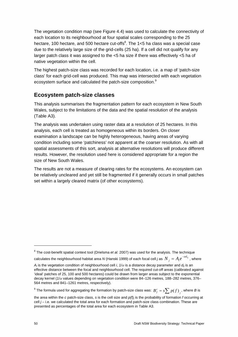
50 Draft NSW Biodiversity Strategy: Technical Paper
The vegetation condition map (see Figure 4.4) was used to calculate the connectivity of each location to its neighbourhood at four spatial scales corresponding to the 25 hectare, 100 hectare, and 500 hectare cut-offs8. The 1<5 ha class was a special case due to the relatively large size of the grid-cells (25 ha). If a cell did not qualify for any larger patch class it was assigned to the <5 ha size if there was effectively <5 ha of native vegetation within the cell.
The highest patch-size class was recorded for each location, i.e. a map of ‘patch-size class’ for each grid-cell was produced. This map was intersected with each vegetation ecosystem surface and calculated the patch-size composition.9
Ecosystem patch-size classes This analysis summarises the fragmentation pattern for each ecosystem in New South Wales, subject to the limitations of the data and the spatial resolution of the analysis (Table A3).
The analysis was undertaken using raster data at a resolution of 25 hectares. In this analysis, each cell is treated as homogeneous within its borders. On closer examination a landscape can be highly heterogeneous, having areas of varying condition including some ‘patchiness’ not apparent at the coarser resolution. As with all spatial assessments of this sort, analysis at alternative resolutions will produce different results. However, the resolution used here is considered appropriate for a region the size of New South Wales.
The results are not a measure of clearing rates for the ecosystems. An ecosystem can be relatively uncleared and yet still be fragmented if it generally occurs in small patches set within a largely cleared matrix (of other ecosystems).
8 The cost-benefit spatial context tool (Drielsma et al. 2007) was used for the analysis. The technique
calculates the neighbourhood habitat area N (Hanski 1999) of each focal cell j as ijdij eAN α−= , where
Ai is the vegetation condition of neighbourhood cell i, 1/α is a distance decay parameter and dij is an effective distance between the focal and neighbourhood cell. The required cut-off areas (calibrated against ‘ideal’ patches of 25, 100 and 500 hectares) could be drawn from larger areas subject to the exponential decay kernel (1/α values depending on vegetation condition were 84–126 metres, 188–282 metres, 376–564 metres and 841–1261 metres, respectively). 9 The formula used for aggregating the formation by patch-size class was:
jcf fpsB ∑= )( , where B is
the area within the c patch-size class, s is the cell size and p(f)j is the probability of formation f occurring at cell j – i.e. we calculated the total area for each formation and patch-size class combination. These are presented as percentages of the total area for each ecosystem in Table A3.
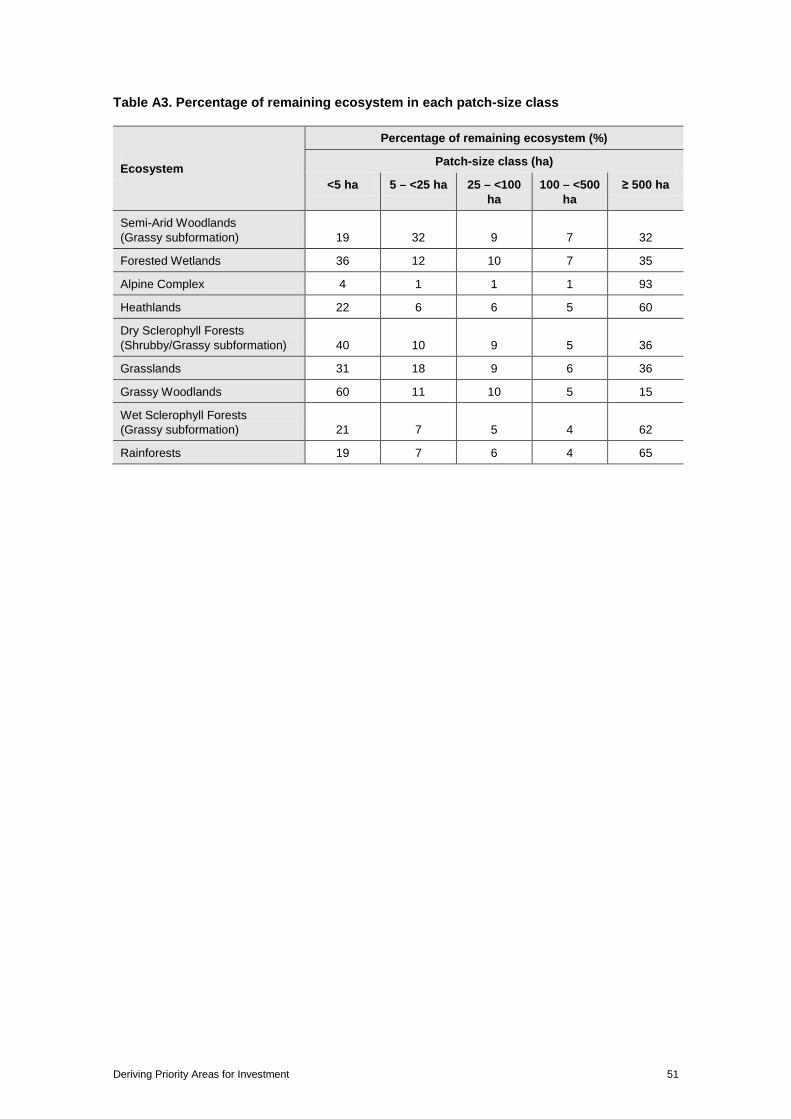
Deriving Priority Areas for Investment 51
Table A3. Percentage of remaining ecosystem in each patch-size class
Ecosystem
Percentage of remaining ecosystem (%)
Patch-size class (ha)
<5 ha 5 – <25 ha 25 – <100 ha
100 – <500 ha
≥ 500 ha
Semi-Arid Woodlands (Grassy subformation) 19 32 9 7 32
Forested Wetlands 36 12 10 7 35
Alpine Complex 4 1 1 1 93
Heathlands 22 6 6 5 60
Dry Sclerophyll Forests (Shrubby/Grassy subformation) 40 10 9 5 36
Grasslands 31 18 9 6 36
Grassy Woodlands 60 11 10 5 15
Wet Sclerophyll Forests (Grassy subformation) 21 7 5 4 62
Rainforests 19 7 6 4 65
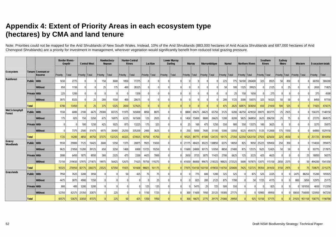
52 Draft NSW Biodiversity Strategy: Technical Paper
Appendix 4: Extent of Priority Areas in each ecosystem type (hectares) by CMA and land tenure Note: Priorities could not be mapped for the Arid Shrublands of New South Wales. Instead, 10% of the Arid Shrublands (883,000 hectares of Arid Acacia Shrublands and 687,000 hectares of Arid Chenopod Shrublands) are a priority for investment in management, wherever vegetation would significantly benefit from reduced total grazing pressure.
Ecosystem
Tenure
Covenant or Reserve
Border Rivers-Gwydir Central West
Hawkesbury-Nepean
Hunter-Central Rivers Lachlan
Lower Murray Darling Murray Murrumbidgee Namoi Northern Rivers
Southern Rivers
Sydney Metro Western Ecosystem totals
Priority Total Priority Total Priority Total Priority Total Priority Total Priority Total Priority Total Priority Total Priority Total Priority Total Priority Total Priority Total Priority Total Priority Total Rainforest Public With 1650 2775 0 0 150 3600 1850 77275 0 0 0 0 0 0 0 0 225 775 56100 206400 325 8925 50 450 0 0 60350 300200
Without 850 1150 0 0 25 175 400 28325 0 0 0 0 0 0 0 0 50 100 1325 39925 0 2125 0 25 0 0 2650 71825
Private With 225 1200 0 0 0 0 0 1350 0 0 0 0 0 0 0 0 0 25 150 1650 0 275 0 0 0 0 375 4500
Without 3975 8325 0 25 200 1550 400 20675 0 0 0 0 0 0 0 0 200 1725 3300 55075 325 10325 50 50 0 0 8450 97750
Total 6700 13450 0 25 375 5325 2650 127625 0 0 0 0 0 0 0 0 475 2625 60875 303050 650 21650 100 525 0 0 71825 474275 Wet Sclerophyll Forest Public With 1550 6000 2100 6675 29300 83725 11975 165000 8050 8875 0 0 8800 69675 24625 65750 3125 6200 46750 429550 20075 303775 25 2925 0 0 156375 1148150
Without 175 825 150 5350 675 16975 6225 161500 125 2925 0 0 1450 15000 8800 26625 1200 8200 5825 360850 2625 206250 25 75 0 0 27275 804575
Private With 0 0 100 1250 425 1025 875 13225 175 325 0 0 25 100 475 1250 550 900 550 13375 100 3625 0 0 0 0 3275 35075
Without 0 7375 2500 31475 6975 30400 25250 335200 2400 3625 0 0 250 5000 7600 31100 5300 12050 9225 459375 5125 112000 175 1550 0 0 64800 1029150
Total 1725 14200 4850 44750 37375 132125 44325 674925 10750 15750 0 0 10525 89775 41500 124725 10175 27350 62350 1263150 27925 625650 225 4550 0 0 251725 3016950 Grassy Woodlands Public With 9550 29000 7125 16425 2600 5350 1375 20875 9925 15650 0 0 21175 40425 30225 138850 6375 14050 825 9050 25225 109450 250 350 0 0 114650 399475
Without 9625 21850 15200 39125 650 3250 1400 6900 13725 19250 0 0 11600 24000 30175 51050 8850 27400 875 12575 1625 12425 50 50 0 0 93775 217875
Private With 2000 6450 1875 8950 300 2325 475 2200 4425 7000 0 0 2650 3725 3075 11425 2700 6625 125 3225 425 4625 0 0 0 25 18050 56575
Without 72150 219650 57975 271875 19975 56425 12675 71625 70750 119275 0 0 41650 86000 99675 218325 98825 272525 5600 107875 12075 115150 2850 2575 0 50 494200 1541350
Total 93325 276950 82175 336375 23525 67350 15925 101600 98825 161175 0 0 77075 154150 163150 419650 116750 320600 7425 132725 39350 241650 3150 2975 0 75 720675 2215275 Grasslands Public With 7950 7625 3200 3950 0 0 50 425 75 75 0 0 0 775 600 1200 325 525 0 875 525 2225 0 0 2475 88250 15200 105925
Without 4475 3075 4900 7350 0 0 0 0 0 25 0 0 0 825 200 2125 875 1700 0 50 1725 4175 0 0 800 5850 12975 25175
Private With 800 400 3200 3200 0 0 0 0 125 125 0 0 0 5475 25 725 500 550 0 0 0 825 0 0 0 101050 4650 112350
Without 52350 42575 21350 32875 0 225 0 0 1150 1725 0 0 300 11600 1950 25125 19300 27175 0 0 10900 49950 0 0 18650 756000 125950 947250
Total 65575 53675 32650 47375 0 225 50 425 1350 1950 0 0 300 18675 2775 29175 21000 29950 0 925 13150 57175 0 0 21925 951150 158775 1190700
Deriving Priority Areas for Investment 53
Ecosystem
Tenure
Covenant or Reserve
Border Rivers-Gwydir Central West
Hawkesbury-Nepean
Hunter-Central Rivers Lachlan
Lower Murray Darling Murray Murrumbidgee Namoi Northern Rivers
Southern Rivers
Sydney Metro Western Ecosystem totals
Priority Total Priority Total Priority Total Priority Total Priority Total Priority Total Priority Total Priority Total Priority Total Priority Total Priority Total Priority Total Priority Total Priority Total Dry Sclerophyll Forest Public With 26875 198400 40100 199550 17700 896075 8575 408725 3850 88900 0 0 19325 69775 13950 180525 27900 318475 8550 435400 3625 562725 0 21150 0 0 170450 3379700
Without 14250 66275 10625 101150 700 69850 1475 70350 1350 31400 0 0 875 6025 2500 40200 5425 277275 1775 228350 325 157300 0 2975 0 0 39300 1051150
Private With 3800 27225 2500 25750 550 11600 650 10825 675 13850 0 0 275 3075 2725 16250 1350 22700 275 22600 150 13625 0 25 0 0 12950 167525
Without 123500 538925 42450 470425 8025 301675 27325 374525 15725 188125 0 0 14800 41850 26850 187575 67725 535675 5100 554075 3775 243075 925 33025 0 0 336200 3468950
Total 168425 830825 95675 796875 26975 1279200 38025 864425 21600 322275 0 0 35275 120725 46025 424550 102400 1154125 15700 1240425 7875 976725 925 57175 0 0 558900 8067325 Heathlands Public With 25 1550 1175 13050 600 33150 150 17000 200 300 0 0 0 0 0 250 75 500 1050 9775 250 47850 350 5700 0 0 3875 129125
Without 25 100 0 4950 0 2150 0 650 25 25 0 0 0 0 0 0 75 225 25 400 25 400 0 0 0 0 175 8900
Private With 0 75 0 275 0 25 0 0 0 125 0 0 0 0 0 0 25 75 0 50 0 200 0 0 0 0 25 825
Without 650 1650 50 6050 0 3250 0 1750 0 50 0 0 0 0 0 0 250 1625 275 2225 225 4925 150 500 0 0 1600 22025
Total 700 3375 1225 24325 600 38575 150 19400 225 500 0 0 0 0 0 250 425 2425 1350 12450 500 53375 500 6200 0 0 5675 160875 Alpine complex Public With 0 0 0 0 0 0 0 0 0 0 0 0 800 39150 5775 49950 0 0 0 0 275 56800 0 0 0 0 6850 145900
Without 0 0 0 0 0 0 0 0 0 0 0 0 0 0 0 0 0 0 0 0 0 750 0 0 0 0 0 750
Private With 0 0 0 0 0 0 0 0 0 0 0 0 0 0 0 0 0 0 0 0 0 0 0 0 0 0 0 0
Without 0 0 0 0 0 0 0 0 0 0 0 0 0 50 0 25 0 0 0 0 25 1250 0 0 0 0 25 1325
Total 0 0 0 0 0 0 0 0 0 0 0 0 800 39200 5775 49975 0 0 0 0 300 58800 0 0 0 0 6875 147975 Semi-arid Woodland Public With 47900 53575 35300 159825 0 0 0 0 1375 339775 14925 360950 5175 9450 20375 39625 39250 38925 0 0 0 0 0 0 8200 783250 172500 1785375
Without 62525 60150 44200 319250 0 0 0 0 1475 106725 17000 58425 7450 14625 5525 35000 42975 29275 0 0 0 0 0 0 1400 93625 182550 717075
Private With 16550 10275 2425 41725 0 0 0 0 1225 36650 0 299900 425 5975 575 9075 2550 3200 0 0 0 0 0 0 0 514525 23750 921325
Without 266300 250175 196100 847700 0 0 0 0 17250 1236400 17850 2807250 23350 84400 26650 195600 138950 115900 0 0 0 0 0 0 80575 7138525 767025 12675950
Total 393275 374175 278025 1368500 0 0 0 0 21325 1719550 49775 3526525 36400 114450 53125 279300 223725 187300 0 0 0 0 0 0 90175 8529925 1145825 16099725 Forested Wetlands Public With 2050 4475 2400 11325 525 2800 1100 22600 1725 6550 4450 10200 32975 49250 18875 31550 1325 6325 12800 54150 850 7425 0 25 25 175 79100 206850
Without 2800 7825 3850 18100 175 1400 525 7200 3125 9125 13400 19450 39200 58575 10275 15125 2050 5750 11125 30950 725 10675 50 100 0 50 87300 184325
Private With 175 400 425 3050 75 175 25 325 1975 4350 25 425 425 12825 1750 2700 300 725 950 2175 0 800 0 0 0 0 6125 27950
Without 9150 23400 10275 59100 2575 7825 3125 43275 19200 59300 12650 40250 24950 100200 23125 51325 9750 18775 28125 95775 2025 17650 525 625 0 650 145475 518150
Total 14175 36100 16950 91575 3350 12200 4775 73400 26025 79325 30525 70325 97550 220850 54025 100700 13425 31575 53000 183050 3600 36550 575 750 25 875 318000 937275
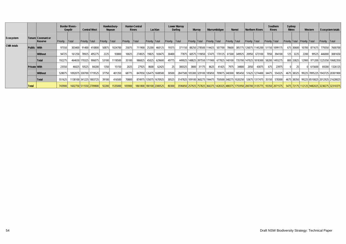
54 Draft NSW Biodiversity Strategy: Technical Paper
Ecosystem
Tenure
Covenant or Reserve
Border Rivers-Gwydir Central West
Hawkesbury-Nepean
Hunter-Central Rivers Lachlan
Lower Murray Darling Murray Murrumbidgee Namoi Northern Rivers
Southern Rivers
Sydney Metro Western Ecosystem totals
Priority Total Priority Total Priority Total Priority Total Priority Total Priority Total Priority Total Priority Total Priority Total Priority Total Priority Total Priority Total Priority Total Priority Total CMA totals Public With 97550 303400 91400 410800 50875 1024700 25075 711900 25200 460125 19375 371150 88250 278500 114425 507700 78600 385775 126075 1145200 51150 1099175 675 30600 10700 871675 779350 7600700
Without 94725 161250 78925 495275 2225 93800 10025 274925 19825 169475 30400 77875 60575 119050 57475 170125 61500 349925 20950 673100 7050 394100 125 3225 2200 99525 446000 3081650
Total 192275 464650 170325 906075 53100 1118500 35100 986825 45025 629600 49775 449025 148825 397550 171900 677825 140100 735700 147025 1818300 58200 1493275 800 33825 12900 971200 1225350 10682350
Private With 23550 46025 10525 84200 1350 15150 2025 27925 8600 62425 25 300325 3800 31175 8625 41425 7975 34800 2050 43075 675 23975 0 25 0 615600 69200 1326125
Without 528075 1092075 330700 1719525 37750 401350 68775 847050 126475 1608500 30500 2847500 105300 329100 185850 709075 340300 985450 51625 1274400 34475 554325 4675 38325 99225 7895225 1943725 20301900
Total 551625 1138100 341225 1803725 39100 416500 70800 874975 135075 1670925 30525 3147825 109100 360275 194475 750500 348275 1020250 53675 1317475 35150 578300 4675 38350 99225 8510825 2012925 21628025
Total 743900 1602750 511550 2709800 92200 1535000 105900 1861800 180100 2300525 80300 3596850 257925 757825 366375 1428325 488375 1755950 200700 3135775 93350 2071575 5475 72175 112125 9482025 3238275 32310375


www.environment.nsw.gov.au


