PROTEINS Structure, Function, and Genetics 6:46-60 (1989) Describing Protein Structure: A General Algorithm Yielding Complete Helicoidal Parameters and a Unique Overall Axis Heinz Sklenar,' Catherine Etchebest? and Richard Lavery2 'Central Institute of Molecular Biology, Academy of Sciences of the GDR, Robert Rossle Strasse 10, DDR -1 115 Berlin Buch, German Democratic Republic, and 'Institut de Biologie Physico-Chimique, 13 rue Pierre et Marie Curie, Paris 75005, France ABSTRACT We present a general and mathematically rigorous algorithm which al- lows the helicoidal structure of a protein to be calculated starting from the atomic coordinates of its peptide backbone. This algorithm yields a unique curved axis which quantifies the folding of the backbone and a full set of helicoidal pa- rameters describing the location of each pep- tide unit. The parameters obtained form a com- plete and independent set and can therefore be used for analyzing, comparing, or reconstruct- ing protein backbone geometry. This algorithm has been implemented in a computer program named P-Curve. Several examples of its possi- ble applications are discussed. Key words: macromolecular conformation, protein folding, helical axis, sec- ondary structure INTRODUCTION The increasing number of well-resolved protein structures available today poses the problem of how the conformations of these often very complex mac- romolecules can best be described. The simplest and most common solution to this problem is based on the calculation of the backbone and side chain tor- sion angles. In the case of the backbone, a Rama- chandran plot' of +I$ torsions can subsequently in- dicate roughly the zones involved in recognizable secondary structure motifs such as a-helices or p- sheets. However, this approach cannot easily de- scribe the folding of the protein backbone and is not very useful for finer studies such as the comparison of homologous structures, the description of turns, or the exact delimitation of secondary structures and detection of their internal distortions. A number of partial solutions to these different problems have been but no completely satisfactory description of protein backbone struc- ture has yet been put forward. One attempt at an overall description has been made by Rackovsky and Scheraga7-' using differential geometry to obtain a continuous space curve based on the positions of suc- cessive C-a backbone atoms. This description, how- 0 1989 ALAN R. LISS, INC. ever, cannot be considered an ideal representation of folding since it remains curved and twisted even within secondary structure zones and thus renders the identification of real backbone kinks or turns difficult. Moreover, the resolution of the method for detecting secondary structures is limited by the fact that a minimum of four a carbons is necessary to obtain the parameters describing the form of the space curve. The only way to overcome these difficulties ap- pears to be the description of the protein backbone in terms of a rigorous definition of a generalized helical axis. This solution has the advantage of leading to a very simple and clear description of folding, since the backbones of all secondary structure zones will be reduced to more or less straight lines and true kinks or turns will be clearly visualized. Moreover, this approach, which must be based on the spacial location of successive peptides in the protein back- bone, will enable a complete parameter set to be obtained for each monomeric unit. Two attempts to obtain at least approximate he- lical axes for proteins or protein fragments have al- ready been made.l0-l2 These approaches are both based on the least-squares fitting of short probe he- lices to successive groups of backbone atoms within the proteins studied. In the work of Barlow and Thornton" an approximate overall helical axis is then defined by linking together successive loca- tions on the probe axes. The disadvantage of this work is first, its approximate nature, the results ob- tained depending on both the length and the confor- mation of the probe helix employed. In addition, while regular secondary structure zones can be treated with this technique, extension of the analy- sis to irregular coil regions or sharp turns is much less obvious. This situation clearly hinders a deeper under- Received February 2, 1989; revision accepted May 30, 1989. Address reprint requests to R. Lavery, Institut de Biologie Physico-Chimique, 13 rue Pierre et Marie Curie, Paris 75005, France.
Transcript
PROTEINS Structure, Function, and Genetics 6:46-60 (1989)
Describing Protein Structure: A General Algorithm Yielding Complete Helicoidal Parameters and a Unique Overall Axis Heinz Sklenar,' Catherine Etchebest? and Richard Lavery2 'Central Institute of Molecular Biology, Academy of Sciences of the GDR, Robert Rossle Strasse 10, DDR -1 115 Berlin Buch, German Democratic Republic, and 'Institut de Biologie Physico-Chimique, 13 rue Pierre et Marie Curie, Paris 75005, France
ABSTRACT We present a general and mathematically rigorous algorithm which al- lows the helicoidal structure of a protein to be calculated starting from the atomic coordinates of its peptide backbone. This algorithm yields a unique curved axis which quantifies the folding of the backbone and a full set of helicoidal pa- rameters describing the location of each pep- tide unit. The parameters obtained form a com- plete and independent set and can therefore be used for analyzing, comparing, or reconstruct- ing protein backbone geometry. This algorithm has been implemented in a computer program named P-Curve. Several examples of its possi- ble applications are discussed.
The increasing number of well-resolved protein structures available today poses the problem of how the conformations of these often very complex mac- romolecules can best be described. The simplest and most common solution to this problem is based on the calculation of the backbone and side chain tor- sion angles. In the case of the backbone, a Rama- chandran plot' of +I$ torsions can subsequently in- dicate roughly the zones involved in recognizable secondary structure motifs such as a-helices or p- sheets. However, this approach cannot easily de- scribe the folding of the protein backbone and is not very useful for finer studies such as the comparison of homologous structures, the description of turns, or the exact delimitation of secondary structures and detection of their internal distortions.
A number of partial solutions to these different problems have been but no completely satisfactory description of protein backbone struc- ture has yet been put forward. One attempt at an overall description has been made by Rackovsky and Scheraga7-' using differential geometry t o obtain a continuous space curve based on the positions of suc- cessive C-a backbone atoms. This description, how-
0 1989 ALAN R. LISS, INC.
ever, cannot be considered an ideal representation of folding since it remains curved and twisted even within secondary structure zones and thus renders the identification of real backbone kinks or turns difficult. Moreover, the resolution of the method for detecting secondary structures is limited by the fact that a minimum of four a carbons is necessary to obtain the parameters describing the form of the space curve.
The only way to overcome these difficulties ap- pears t o be the description of the protein backbone in terms of a rigorous definition of a generalized helical axis. This solution has the advantage of leading to a very simple and clear description of folding, since the backbones of all secondary structure zones will be reduced to more or less straight lines and true kinks or turns will be clearly visualized. Moreover, this approach, which must be based on the spacial location of successive peptides in the protein back- bone, will enable a complete parameter set to be obtained for each monomeric unit.
Two attempts to obtain at least approximate he- lical axes for proteins or protein fragments have al- ready been made.l0-l2 These approaches are both based on the least-squares fitting of short probe he- lices to successive groups of backbone atoms within the proteins studied. In the work of Barlow and Thornton" an approximate overall helical axis is then defined by linking together successive loca- tions on the probe axes. The disadvantage of this work is first, its approximate nature, the results ob- tained depending on both the length and the confor- mation of the probe helix employed. In addition, while regular secondary structure zones can be treated with this technique, extension of the analy- sis to irregular coil regions or sharp turns is much less obvious.
This situation clearly hinders a deeper under-
Received February 2, 1989; revision accepted May 30, 1989. Address reprint requests to R. Lavery, Institut de Biologie
Physico-Chimique, 13 rue Pierre et Marie Curie, Paris 75005, France.
AN ALGORITHM FOR DESCRIBING PROTEIN STRUCTURE
I N terrninol I f-
H
\
I ,N"-l
I I
Fig. 1. Division of the polypeptide backbone for helical analysis. The mth unit is indicated by the dotted lines and comprises the peptide plane defined by C;, and Nm+,
47
Fig. 2. Definition of the peptide fixed axis system j K i . €is the mid-point of the peptide bond and the plane shown corresponds to the mean plane of the peptide group.
Fig. 4. Construction of the mean plane used for calculating interpeptide parameters.
- Pi
Fig. 3. Definition of the helicoidal parameters (X displace- ment, Y displacement, inclination. and tip) which re!a!e_the peptide axis system JKL to the local helical axis system VWU
standing of protein folding and limits the amount of data which can easily be extracted from data banks of protein structure. We would like to propose a pos- sible solution to this problem by describing a gen- eral algorithm which can be used to obtain a com- plete and unique helicoidal description of any protein backbone. The algorithm we will describe is an adaption of the approach we have recently devel- oped for describing nucleic acid s t r ~ c t u r e . ' ~ , ~ ~ It leads to a unique curved helicoidal axis and a full set of helicoidal parameters which locate each peptide unit with respect to this axis and with respect to its neighbors.
Our method is a natural extension of the defini- tions used in helical descriptions of regular poly- mers to the case of irregular systems. The basis of this approach is the definition of a function which
f a .-
AN ALGORITHM FOR DESCRIBING PROTEIN STRUCTURE 49
describes departure from perfect helical symmetry in terms of the curvature of the axis describing the polymer and in terms of changes in the position of successive monomers with respect to this axis. Min- imization of this geometric function yields the gen- erally curved axis of the polymer and provides a unique helical description where both types of irreg- ularity have been "smoothed" in an optimal least- squares sense. Since the function is constructed so as to take into account simultaneously the position of all the monomeric units making up the polymer, the final description of any one of these units thus de- pends on the position of its neighbors. This leads to a much more coherent view of the overall conforma- tion than that obtained with any purely local pa- rameters such as the backbone torsion angles.
Once the analysis has been performed for a given protein, a great deal of information on its conforma- tion can be obtained. It now becomes possible to rig- orously define the location of secondary structures
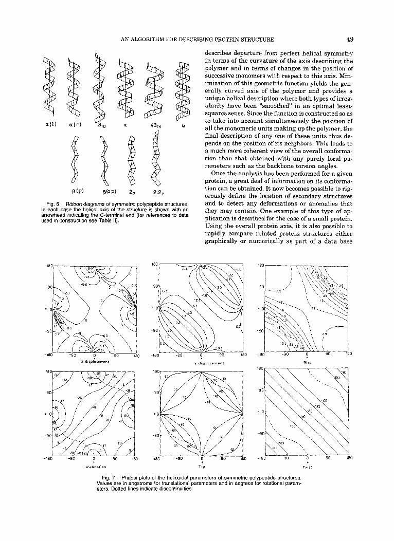
Fio. 6. Ribbon diaorams of svmmetric oolvoeotide structures. and to detect any deformations or anomalies that In each case the helGal axis Oi the strudtur;?' is' shown with an they may contain. One example of this type of ap- arrowhead indicating the C-terminal end (for references to data used in construction see Table 11). plication is described for the case of a small protein.
Using the overall protein axis, it is also possible to rapidly compare related protein structures either graphically or numerically as part of a data base
180 180
90 90
-90 - 90
-90 90 0 0, I80 -180
Y disolocement x displocement
+ b + I " C i i " O l l 0 " Tip Tnisl
Fig. 7. Phi/psi plots of the helicoidal parameters of symmetric polypeptide structures. Values are in angstroms for translational parameters and in degrees for rotational param- eters. Dotted lines indicate discontinuities.
50 H. SKLENAR E T AL.
Fig. 8. Stereodiagrams of the helical axis alone (above) and of the backbone ribbon and the helical axis (below) resulting from the analysis of crarnbin (coordinates from ref. 19).
search program. Moreover, since this axis is a well- defined and concise alternative to the C-a backbone curve for describing the path of the polymer chain, the apparatus of differential geometry can be used to describe its shape in the same way as proposed by Rackovsky and S ~ h e r a g a . ~ We will not make such an analysis presently, but will consider this possi- bility in our forthcoming studies.
MATERIALS AND METHODS The first step in defining the helicoidal structure of
a polymer is to choose the structural repeating ele- ment to be used. For a protein the most natural choice seems to be the successive peptide groups. For the purposes of our analysis we will consequently divide the protein chain as shown in Figure 1. We must
subsequently associate a fixed axis system with each repeating element, which will serve to define its po- sition in space. This axis system is shown in Figure 2 . It is centered on the middle of the peptide bond @I and defined by three mutually perpendicular unit vectors (J ,KL) . The first of these vectors, J , is simply the peptide bond vector in the direction N-C’. L lies in the mean plane of the peptide group and points toward the side carrying the carbonyl group. K is perpendicular to the mean peptide plane, and is de- fined by the vector product L x 3.
Next, it is necessary to define the position of each repeating element with respect to a local helical axis system. This requires four variables, two transla- tions and two rotations. These variables are shown in Figure 3. The helical axis system is centered at point
AN ALGORITHM FOR DESCRIBING PROTEIN STRUCTURE 51
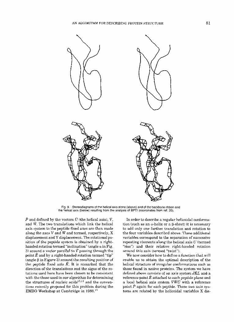
Fig. g.-Stereodiagrarns of the helical axis alone (above) and of the backbone ribbon and the helical axis (below) resulting from the analysis of BPTl (coordinates from ref. 20).
P and defined by the vectors U (the helical axis), V, and W. The two translations which link the helical axis system to the peptide fixed axes are then made along the axes V and W and termed, respectively, X displacement and Y displacement. The rotational po- sition of the peptide system is obtained by a right- handed rotation termed “inclination” (angle a in Fig. 3) around a vector parallel to V passing through the point E and by a right-handed rotation termed “tip” (angle P in Figure 3) around the resulting position of the peptide fixed axis K. It is remarked that the direction of the translations and the signs of the ro- tations used here have been chosen to be consistent with the those used in our algorithm for determining the structures of nucleic a c i d ~ l ~ , ’ ~ and the conven- tions recently proposed for this problem during the EMBO Workshop a t Cambridge in 1988.15
In order to describe a regular helicoidal conforma- tion (such as an a-helix or a P-sheet) it is necessary to add only one further translation and rotation to the four variables described above. These additional variables correspond to the separation of successive repeating elements along the helical axis U (termed “rise”) and their relative right-handed rotation around this axis (termed “twist”).
We now consider how to define a function that will enable us to obtain the optimal description of the helical structure of irregular conformations such as those found in native proteins. The system we have defined above consists of an axis system JKL and a reference point E attached to each peptide plane and a local helical axis system VWU with a reference point P again for each peptide. These two axis sys- tems are related by the helicoidal variables X dis-
_ _ _
52 H. SKLENAR ET AL.
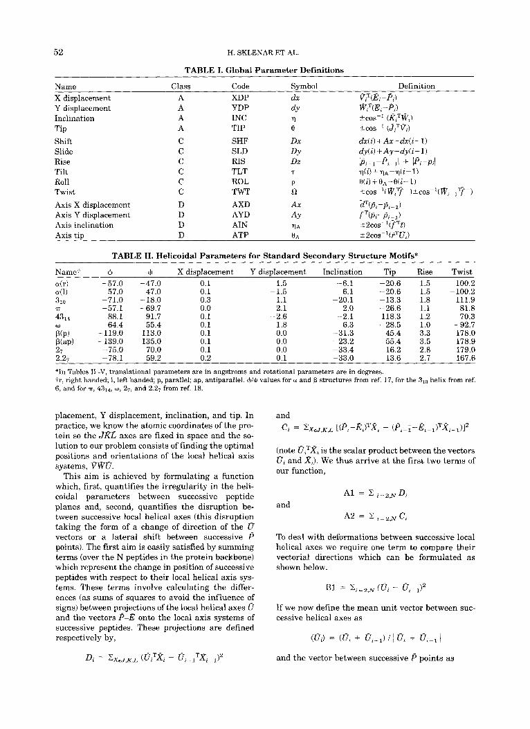
TABLE I. Global Parameter Definitions
Name Class Code Symbol Definition X displacement A XDP dx V',T(EL -P;) Y displacement A YDP dY W m ? , - P J Inclination A INC rl kcOs-1 (KiTWL)
Tip A TIP 0 2 cos-1 (J,TVJ
Rise C RIS Dz bi-l-Pz-ll + /P,-P,I Tilt C TLT 7 V ( i ) +.Yl-rl(i-l) Roll C ROL P O ( i ) +0,-B(i- l )
Axis X displacement D AXD A x Z(Pz-P;-J Axis Y displacement D AYD AY fT(PL-Pj- 1) Axis inclination D AIN YA 42cos-'(fTt) Axis tip D ATP HA 2 2cos-l(T=TU,)
Shift C SHF D x dx( i )+Ax-dx( i - l ) Slide C SLD DY dy(i) + Ay-dy( i- 1)
C TWT 0 +cos-l - (Wj - T- f + )kcos-l(WL-lTf-) Twist
TABLE 11. Helicoidal Parameters for Standard Secondary Structure Motifs*
Name: + JI X displacement Y displacement Inclination Tip Rise Twist a(r) -57.0 -47.0 0.1 1.5 -6.1 -20.6 1.5 100.2 ail) 57.0 47.0 0.1 310 -71.0 -18.0 0.3 7T -57.1 -69.7 0.0 4314 88.1 91.7 0.1 w 64.4 55.4 0.1 P(P) -119.0 113.0 0.1 P b P ) -139.0 135.0 0.1 27 -75.0 70.0 0.1 2.Z7 -78.1 59.2 0.2
*In Tables 11-V, translational parameters are in angstroms and rotational parameters are in degrees. t r , right handed; 1, left handed; p, parallel; ap, antiparallel. $J/$ values for oi and p structures from ref. 17, for the 310 helix from ref. 6, and for 7, 4314, to, 27, and 2.27 from ref. 18.
placement, Y displacement, inclination, and tip. In practice, we know the atomic coordinates of the pro- tein so the JKL axes are fixed in space and the so- lution to our problem consists of finding the optimal positions and orientations of the local helical axis systems, VWU.
This aim is achieved by formulating a function which, first, quantifies the irregularity in the heli- coidal parameters between successive peptide planes and, second, quantifies the disruption be- tween successive local helical axes (this disruption taking the form of a change of direction of the U vectors or a lateral shift between successive P points). The first aim is easily satisfied by summing terms (over the N peptides in the protein backbone) which represent the change in position of successive peptides with respect to their local helical axis sys- tems. These terms involve calculating the differ- ences (as sums of squares to avoid the influence of signs) between projections of the local helical axes 0 and the vectors P-E onto the local axis systems of successive peptides. These projections are defined respectively by,
(note UiTXi is the scalar product between the vectors U i and X i ) . We thus arrive a t the first two terms of our function.
To deal with deformations between successive local helical axes we require one term to compare their vectorial directions which can be formulated as shown below.
If we now define the mean unit vector between suc- cessive helical axes as
(U,) = (0, + ui-l) I ~ 0, + Oipl ~
and the vector between successive P points as
AN ALGORITHM FOR DESCRIBING PROTEIN STRUCTURE 53
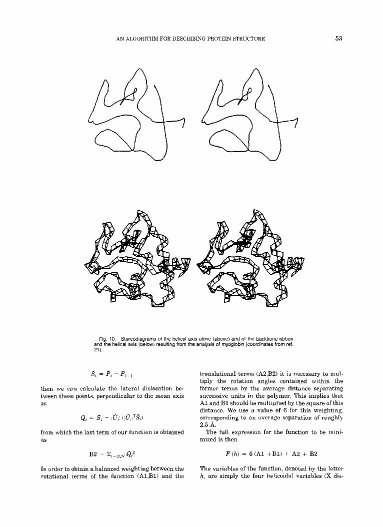
Fig. 10. Stereodiagrams of the helical axis alone (above) and of the backbone ribbon and the helical axis (below) resulting from the analysis of myoglobin (coordinates from ref. 21).
s, = Pi - P,&l
then we can calculate the lateral dislocation be- tween these points, perpendicular to the mean axis as
from which the last term of our function is obtained as
In order to obtain a balanced weighting between the rotational terms of the function (A1,Bl) and the
translational terms (A2,B2) it is necessary t o mul- tiply the rotation angles contained within the former terms by the average distance separating successive units in the polymer. This implies that A1 and B1 should be multiplied by the square of this distance. We use a value of 6 for this weighting, corresponding to an average separation of roughly 2.5 A.
The full expression for the function to be mini- mized is then
F ( h ) = 6 (A1 +B1) + A2 + B2
The variables of the function, denoted by the letter h, are simply the four helicoidal variables (X dis-
54 H. SKLENAR ET AL
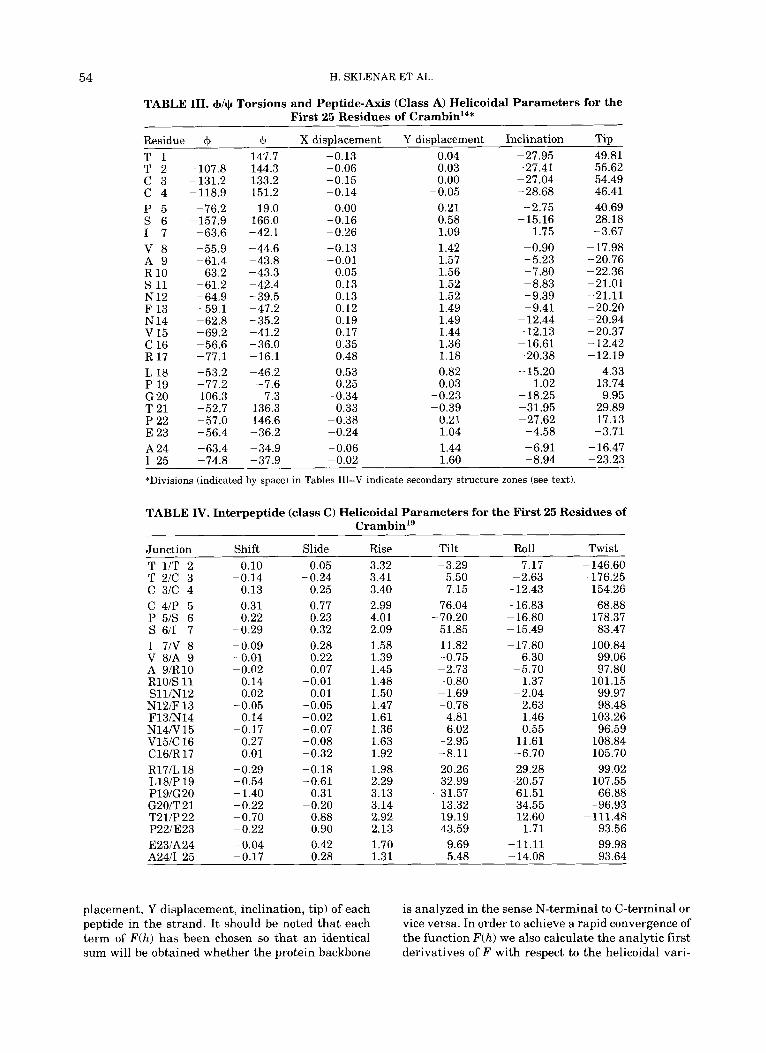
TABLE 111. +/+ Torsions and Peptide-Axis (Class A) Helicoidal Parameters for the First 25 Residues of CrambinI4*
T 1 T 2 c 3 c 4 P 5 S 6 I 7 V 8 A 9 R 10 s 11 N 12 F 13 N 14 V 15 C 16 R 17 L 18 P 19 G 20 T 21 P 22 E 23 A24 I 25
placement, Y displacement, inclination, tip) of each peptide in the strand. It should be noted that each term of F(h) has been chosen so that an identical sum will be obtained whether the protein backbone
is analyzed in the sense N-terminal to C-terminal or vice versa. In order to achieve a rapid convergence of the function F(h) we also calculate the analytic first derivatives of F with respect to the helicoidal vari-
AN ALGORITHM FOR DESCRIBING PROTEIN STRUCTURE
TABLE V. Interaxis (Class D) Helicoidal Parameters for the First 25 Residues of CrambinIg
55
Junction Ax AY Ainc Atip Adis Bend T llT 2 0.03 0.06 -3.84 1.35 0.07 4.07 T 21C 3 c 3lC 4 c 41P 5 P 51s 6 S 611 7 I 71V 8 V 81A 9 A 9lR10 RlOlS 11 Sll/N12 Nl2iF 13 F13lN14 N14lV15 V15IC 16 C16lR17 R17IL 18 L18/P 19 P19lG20 G20lT21 T21lP 22 P22lE 23 E23lA24 A2411 25
ables of each peptide. The development of these de- rivatives has been fully described in our previous p~bl icat ion '~ and is not repeated here.
Finally, we must consider the definition of the in- terpeptide parameters in the general case where the local helical axes are not aligned. In this event, the simple definitions of rise and twist given earlier no longer apply and we must also be able to describe the relative position of the two helical axes in space. This is done using a mean axis system (ri,d,fcen- tered a t point 8) as shown in Figure 4. This system is defined by the equations below.
f = , x d
The intersection of the U vectors with the mean plane (perpendicular to A) are then
We can now derive expressions for parameters de- scribing the relative position of the helical axis sys-
tems a t this junction. Two translations along the d and f axes are defined as
Axis X displacement = 2 T(pl - P 1 - l )
Axis Y displacement = f T (p , -
Similarly, two rotations, analogous to inclination and tip, are defined as
axis inclination = 2 c0s-l (f' t), + positive if$ gcx i ) > O
axis tip = 2 c0s-l (F'U,), positive if F(i. x U,) > o
where f = (u, x d)/ U, x dl and i = (d x A/ Id x il.
It is also possible to derive three subsidiary parameters which can be useful. These para- meters measure the net angle formed between successive helical axis vectors [axis bend, Ab = ~ o s - ~ ( U , - , ~ ~ , ) ] , the net lateral dislocation between successive P points [axis dislocation, Ad = d m , and the distance between suc- cessive P points (path length, path = ~ P , - PC-, I 1.
Lastly, we can define the general parameters for the interpeptide junction by three translations:
shift = d3c (i) + Ax - dx (i-1)
56 H. SKLENAR ET AL.
Residue
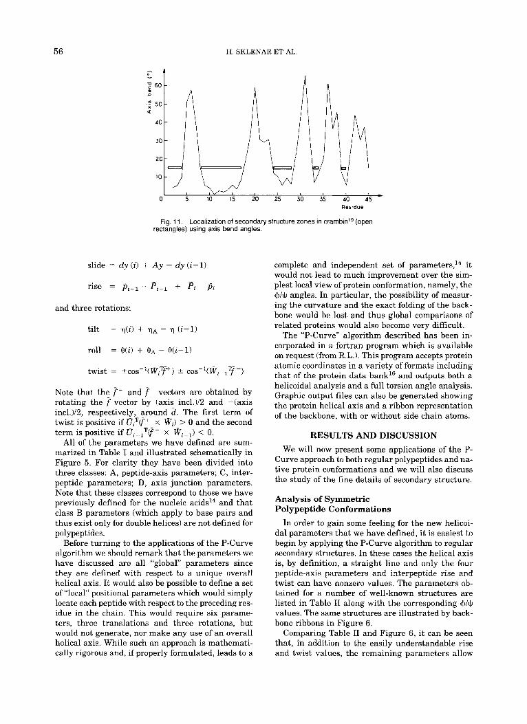
Fig. 11. Localization of secondary structure zones in ~ ra rnb in ’~ (open rectangles) using axis bend angles.
slide = d y ( i ) + A y - dy(i-1)
and three rotations:
roll = O(i) + OA - O(i-1)
Note that the f + and f - vectors are obtained by rotating the f vector by (axis incl.)/2 and -(axis incl.)/2, respectively, around d . The first term of twist is positive if O?(f+ x W J > 0 and the second term is positive if O,-lT(f- x Wz-l) < 0.
All of the parameters we have defined are sum- marized in Table I and illustrated schematically in Figure 5 . For clarity they have been divided into three classes: A, peptide-axis parameters; C, inter- peptide parameters; D, axis junction parameters. Note that these classes correspond to those we have previously defined for the nucleic acidsI4 and that class B parameters (which apply to base pairs and thus exist only for double helices) are not defined for polypeptides.
Before turning to the applications of the P-Curve algorithm we should remark that the parameters we have discussed are all “global” parameters since they are defined with respect to a unique overall helical axis. It would also be possible to define a set of “local” positional parameters which would simply locate each peptide with respect to the preceding res- idue in the chain. This would require six parame- ters, three translations and three rotations, but would not generate, nor make any use of an overall helical axis. While such an approach is mathemati- cally rigorous and, if properly formulated, leads to a
complete and independent set of parameters,’* it would not lead to much improvement over the sim- plest local view of protein conformation, namely, the +/+ angles. In particular, the possibility of measur- ing the curvature and the exact folding of the back- bone would be lost and thus global comparisons of related proteins would also become very difficult.
The “P-Curve” algorithm described has been in- corporated in a fortran program which is available on request (from R.L.). This program accepts protein atomic coordinates in a variety of formats including that of the protein data bank16 and outputs both a helicoidal analysis and a full torsion angle analysis. Graphic output files can also be generated showing the protein helical axis and a ribbon representation of the backbone, with or without side chain atoms.
RESULTS AND DISCUSSION We will now present some applications of the P-
Curve approach to both regular polypeptides and na- tive protein conformations and we will also discuss the study of the fine details of secondary structure.
Analysis of Symmetric Polypeptide Conformations
In order to gain some feeling for the new helicoi- dal parameters that we have defined, it is easiest to begin by applying the P-Curve algorithm to regular secondary structures. In these cases the helical axis is, by definition, a straight line and only the four peptide-axis parameters and interpeptide rise and twist can have nonzero values. The parameters ob- tained for a number of well-known structures are listed in Table I1 along with the corresponding I$/$ values. The same structures are illustrated by back- bone ribbons in Figure 6.
Comparing Table I1 and Figure 6, it can be seen that, in addition to the easily understandable rise and twist values, the remaining parameters allow
AN ALGORITHM FOR DESCRIBING PROTEIN STRUCTURE 57
o.4\ 12
- 1 i
- O . ’ t I -o,2t I
/-
Fig. 12. Variation of the helicoidal parameters of the terminal residue of an a-helix (residues 58-77) extracted from oxymyoglobin2’ as a function of the limit of the P-Curve analysis in the C-terminal direction.
us to judge the radius of the helical structure (al- most directly equal Y displacement, since X dis- placement values tend to be very small) and also of the orientation of the peptide plane with respect to the helical axis, through the inclination and tip val- ues.
Since regular structures naturally lead to regular helicoidal parameters it is also possible to make +/+ plots of these parameters for the full range of the backbone torsion angles. The results of such a study are presented in Figure 7. From these data it is pos- sible to see immediately what type of structure will result for any given +I$ combination and to deter- mine the correlations which exist between the dif- ferent helicoidal parameters.
It should be mentioned at this point that we have not assumed anything about the nature of the link- ages within the peptide backbone and thus six pa- rameters are necessary to define the position of suc- cessive peptides in space. In fact the chemical bonding within a polypeptide means that there are only two single bond torsions between any two pep- tides and thus we can expect quite strong correla- tions between our six helicoidal parameters. How- ever, in any real protein structure, variations in the peptide bond torsion (0) and in valence angles or bond lengths will mean that these correlations can be only approximate. Thus, a rigorous geometrical description of a protein must nevertheless conserve the full number of variables that we have defined.
It should further be stressed that the unique rela- tionship between the backbone torsions 4 4 and the
helicoidal parameters illustrated by Figure 7 is true only for regular structures. In real proteins the con- formational environment of any given peptide unit (that is to say, the structure adopted by the residues preceding and following the peptide unit considered) will influence the position of its local helical axis, during minimization of the function F(h), and con- sequently its helicoidal parameters. Therefore it is clear that no simple relationship between these pa- rameters and the +/$ values of the peptide can exist. We will return to this point shortly.
Analysis of Native Protein Conformations
We now apply the P-Curve algorithm to protein conformation analysis. Three proteins have been chosen as examples to illustrate the nature of the data which can be obtained: crambin,lg bovine pan- creatic trypsin inhibitor,20 and sperm whale oxy- myoglobin.21 The graphic data resulting from the analysis of these proteins are presented in Figures 8-10 by stereodiagrams of the protein backbone rib- bon with the calculated helical axis and of the heli- cal axis alone. Note that the smooth curve presented for the helical axis is generated by a cubic spline fit to the Pi,oi data obtained from P-Curve.
Figures 8-10 show the visual nature of the results obtained from our algorithm. For any protein, re- gions with regular secondary structures (most com- monly, a-helices and p-sheets) are easily visible as straight portions of the axis. These segments are linked by curved zones corresponding to irregular conformations of the polypeptide backbone. On a
58 H. SKLENAR ET AL
c 0.3-
( a ) ( b l
Fig. 13. Variation of the helicoidal parameters of the terminal residue of a @-sheet (residues 29-35) extracted from BPTIzo as a function of the limit of the P-Curve analysis in the C-terminal direction.
graphics system it is possible to color the axis fol- lowing the type of secondary structure detected and thus to obtain a very simple, but nevertheless rig- orous, description of the folding of the polypeptide chain.
In addition to the graphical data, the P-Curve analysis also lists all the helicoidal parameters de- scribed previously. For reasons of space we can present only a part of these data here. We have cho- sen to discuss the first 25 residues of the smallest protein treated, crambin. The parameters obtained for these residues are listed in Tables 111-V. These results will serve to illustrate how our analysis dif- fers from simple +/$torsion angle or hydrogen bond- ing data.
In order to get a quick idea of the localization of regular secondary structures, the three-dimensional helical axis of crambin shown in Figure 8 can be simplified to two dimensions by plotting the bending angle at each junction of the helical axis. This is shown in Figure 11. Secondary structures are now easily distinguished from irregular zones by the low values of their axis bends. If we place a bar a t 15" bending, we immediately detect five relatively straight zones: 1-4, 8-17, 24-28, 33-34, and 39- 40. (Note from Fig. 1 that the division of the peptide chain we have adopted implies that if an interpep- tide junction i-j is bent, then the peptidej should be included in the irregular zone.)
Looking at the data in Tables 111-V and compar- ing it with the standard structures in Table 11, we can rapidly identify the first three zones as a @-sheet followed by two a-helices (the remaining two zones, not shown in the tables, are again @-sheets). The most useful values for this identification are Y dis- placement, tip, rise, and twist, which all distinguish clearly between a and @ sbructures. Regular zones
may also be detected through the small values of the interpeptide parameters shift, slide, tilt, and roll. However, it should be noted that none of the second- ary structures is quantitatively regular and we will return to the description of distortion within these segments in the following section.
If we compare our findings with those listed by the author of the crystallographic study of crambinlg within the corresponding protein data bank entry, several differences can be found. The original as- signments for secondary structure zones were lim- ited to four segments: 1-4 (@), 7-19 (a), 23-30 (a), and 32-35 (PI. All but the first of these zones is wider than our findings and the last P-sheet we have located was not seen. It is interesting t o look in de- tail at the assignment of the first a-helix with the help of the parameters in Tables 111-V. From these data it would seem the residues 7, 18, and 19 cannot easily be classed as belonging to the helix. All these residues have tip values far from those of the a-helix and Y displacement for 18 and 19 is too small. More- over, the junctions 6-7, 17-18, and 18-19 are all distinctly bent and associated with important tilt and roll values.
Looking at the +/+ values in Table I11 it is easy to see that, in the case of a folded polypeptide chain, there is no longer any precise correlation between the backbone torsions and our helicoidal parame- ters. When the F(h) function of the P-Curve algo- rithm is minimized, the residues preceding and fol- lowing any given peptide group influence its helicoidal parameters. Thus, while at least peptides 7 and 18 can be classed as a-helical on the basis of their +/$ values, they cannot in terms of their heli- coidal parameters.
The effect of neighboring residues in our analysis can be shown clearly if we look at other examples of
AN ALGORITHM FOR DESCRIBING PROTEIN STRUCTURE 59
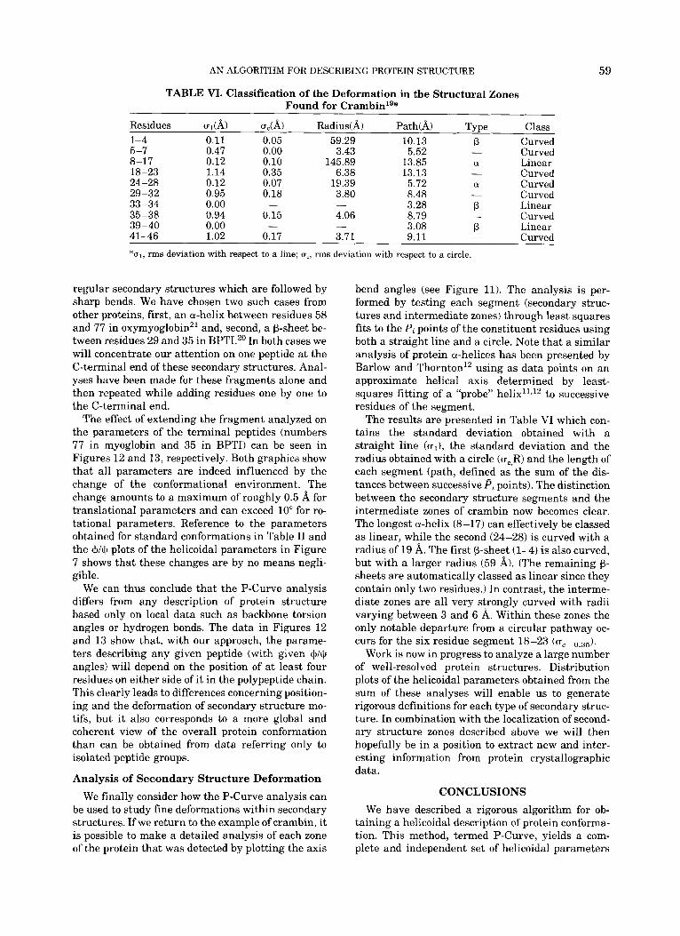
TABLE VI. Classification of the Deformation in the Structural Zones Found for Crambin"*
Residues Ul(A) U,(A) Radius(& Path(& Type Class Curved Curved 5 -7 0.47 0.00 3.43 5.52 -
8-17 0.12 0.10 145.89 13.85 a Linear 18-23 1.14 0.35 6.38 13.13 - Curved 24-28 0.12 0.07 19.39 5.72 a Curved 29-32 0.95 0.18 3.80 8.48 - Curved
Linear Curved
3.28 P 33-34 0.00 - - 35-38 0.94 0.15 4.06 8.79 -
- 3.08 P Linear 39-40 0.00 - 41-46 1.02 0.17 3.71 9.11 - Curved *ul, rms deviation with respect to a line; uc, rms deviation with respect to a circle.
1-4 0.11 0.05 59.29 10.13 P
regular secondary structures which are followed by sharp bends. We have chosen two such cases from other proteins, first, an a-helix between residues 58 and 77 in oxymyoglobinZ1 and, second, a P-sheet be- tween residues 29 and 35 in BPTI.20 In both cases we will concentrate our attention on one peptide at the C-terminal end of these secondary structures. Anal- yses have been made for these fragments alone and then repeated while adding residues one by one to the C-terminal end.
The effect of extending the fragment analyzed on the parameters of the terminal peptides (numbers 77 in myoglobin and 35 in BPTI) can be seen in Figures 12 and 13, respectively. Both graphics show that all parameters are indeed influenced by the change of the conformational environment. The change amounts to a maximum of roughly 0.5 A for translational parameters and can exceed 10" for ro- tational parameters. Reference to the parameters obtained for standard conformations in Table I1 and the +/$ plots of the helicoidal parameters in Figure 7 shows that these changes are by no means negli- gible.
We can thus conclude that the P-Curve analysis differs from any description of protein structure based only on local data such as backbone torsion angles or hydrogen bonds. The data in Figures 12 and 13 show that, with our approach, the parame- ters describing any given peptide (with given +/ti( angles) will depend on the position of at least four residues on either side of it in the polypeptide chain. This clearly leads to differences concerning position- ing and the deformation of secondary structure mo- tifs, but it also corresponds to a more global and coherent view of the overall protein conformation than can be obtained from data referring only to isolated peptide groups.
Analysis of Secondary Structure Deformation We finally consider how the P-Curve analysis can
be used to study fine deformations within secondary structures. If we return to the example of crambin, it is possible to make a detailed analysis of each zone of the protein that was detected by plotting the axis
bend angles (see Figure 11). The analysis is per- formed by testing each segment (secondary struc- tures and intermediate zones) through least squares fits to the P , points of the constituent residues using both a straight line and a circle. Note that a similar analysis of protein a-helices has been presented by Barlow and Thornton12 using as data points on an approximate helical axis determined by least- squares fitting of a "probe" helix11J2 to successive residues of the segment.
The results are presented in Table VI which con- tains the standard deviation obtained with a straight line ((T~), the standard deviation and the radius obtained with a circle (u,,R) and the length of each segment (path, defined as the sum of the dis- tances between successive P i points). The distinction between the secondary structure segments and the intermediate zones of crambin now becomes clear. The longest a-helix (8-17) can effectively be classed as linear, while the second (24-28) is curved with a radius of 19 A. The first P-sheet (1-4) is also curved, but with a larger radius (59 A). (The remaining P- sheets are automatically classed as linear since they contain only two residues.) In contrast, the interme- diate zones are all very strongly curved with radii varying between 3 and 6 A. Within these zones the only notable departure from a circular pathway oc- curs for the six residue segment 18-23 ( I J = ~ . ~ ~ ) .
Work is now in progress to analyze a large number of well-resolved protein structures. Distribution plots of the helicoidal parameters obtained from the sum of these analyses will enable us to generate rigorous definitions for each type of secondary struc- ture. In combination with the localization of second- ary structure zones described above we will then hopefully be in a position to extract new and inter- esting information from protein crystallographic data.
CONCLUSIONS We have described a rigorous algorithm for ob-
taining a helicoidal description of protein conforma- tion. This method, termed P-Curve, yields a com- plete and independent set of helicoidal parameters
60 H. SKLENAR ET AL.
and a unique overall helical axis for any protein whose backbone atomic coordinates are known. The approach makes use of an extended least-squares minimization procedure to yield an optimal helical description where structural irregularities are dis- tributed between changes in the orientation of suc- cessive peptide groups and curvature of the overall helical axis. Using the P-Curve algorithm has two fundamental advantages. First, the algorithm gives a coherent overall view of the entire protein confor- mation and also allows detailed information of the positioning of individual peptides to be extracted. Second, the location of secondary structures and measures of the deformation of these segments or intermediate zones of the backbone can be obtained automatically.
The P-Curve algorithm has obvious applications for describing protein folding patterns and for the automatic comparison of related proteins or searches of chosen conformational fragments within data banks of protein structure. It may also be of considerable interest in analyzing the data from mo- lecular dynamics studies of proteins where the ex- traction of easily readable information is often a ma- jor problem (for a similar application to a nucleic acid oligomer see ref. 22).
1.
2.
3.
4.
5.
6.
7.
REFERENCES Ramakrishnan, C., Ramachandran, G.N. Stereochemical criteria for polypeptide and protein chain conformations 11. Allowed conformations for a pair of peptide units. Biophys. J. 5909-933, 1965. Richardson, J.S. The anatomy and taxonomy of protein structure. Adv. Protein Chem. 34:167-339, 1981. Lifson, S., Sander, C. Specific recognition in the tertiary structure of P-sheets of proteins. J. Mol. Biol. 139:627-639, 1980. Levitt, M., Greer, J . Automatic identification of secondary structure in globular proteins. J . Mol. Biol. 114:181-239, 1977. Kabsch, W., Sander, C . Dictionary of protein secondary structure: Pattern recognition of hydrogen-bonded and geometrical features. Biopolymers 22:2577-2637, 1983. Rose, G.D., Gierasch, L.M., Smith, J.A. Turns in peptides and proteins. Adv. Protein Chem. 37:l-109, 1985. Rackovsky, S., Scheraga, H.A. Differential geometry and
polymer conformation. I. Comparison of protein conforma- tions. Macromolecules 11:1168-1174, 1978.
8. Rackovsky, S., Scheraga, H.A. Differential geometry and polymer conformation. 11. Development of a conforma- tional distance function. Macromolecules 13:1440-1453, 1980.
9. Rackovsky, S., Scheraga, H.A. Differential geometry and polymer conformation. 111. Single-site and nearest- neighbor distributions and nucleation of protein folding. Macromolecules 14:1259-1269, 1981.
11. Blundell, T., Barlow, D., Borakoti, N., Thornton, J. Sol- vent-induced distortions and the curvature of a-helices. Nature (London) 306:281-283, 1983.
12. Barlow, D.J., Thornton, J.M. Helix geometry in proteins. J. Mol. Biol. 201:601-619, 1988.
13. Lavery, R., Sklenar, H. The definition of generalized heli- coidal parameters and of axis curvature for irregular nu- cleic acids. J. Biomol. Struct. Dynam. 663-91, 1988.
14. Lavery, R., Sklenar, H. Defining the structure of irregular nucleic acids: Conventions and principles. J . Biomol. Struct. Dynam. 6:655-667, 1989.
15. Dickerson, R.E., Bansal, M., Calladine, C.R., Diekmann, S., Hunter, W.N., Kennard, O., Lavery, R., Nelson, H.C.M., Olson, W.K., Saenger, W., Shakked, Z., Sklenar, H., Soumpasis, D.M., Tung, C-S., von Kitzing, E., Wang, A.H-J., Zhurkin, V.B. Definitions and nomenclature of nu- cleic acid structure parameters. EMBO J. 8:l-4, 1989; J. Biomol. Struct. Dynam. 6527-634, 1989; J. Mol. Biol. 205: 787-791, 1989.
16. Bernstein, F.C., Koetzle, T.F., Williams, G.J.B., Meyer, E.F., Brice, M.D., Rogers, J.R., Kennard, O., Shimanouchi, T., Tasumi, M. The protein data bank: A computer-based archival file for macromolecular structures. J . Mol. Biol. 112535542, 1977.
17. IUPAC-IUB Commission on biochemical nomenclature. Abbreviations and symbols for the description of the con- formation of polypeptide chains. Biochemistry 9:3471- 3479, 1970 and references therein.
18. Ramachandran, G.N., Sasisekharan, V. Conformation of polypeptides and proteins. Adv. Protein Chem. 23:283- 437, 1983.
19. Teeter, M.M. Water structure of a hydrophobic protein at atomic resolution. Pentagon rings of water molecules in the crystals of crambin. Proc. Natl. Acad. Sci. U.S.A. 81: 6014-6018, 1984.
20. Walter, J., Huber, R. Pancreatic trypsin inhibitor. A new crystal form and its analysis. J . Mol. Biol. 167:911-917, 1983.
21. Phillips, S.E.V. Structure and refinement of oxymyoglobin at 1.6A resolution. J . Mol. Biol. 142:531-554, 1980.
22. Ravishankar, G., Swaminathan, S., Beveridge, D.L., La- very, R., Sklenar, H. Conformational and helicoidal anal- ysis of 30ps of molecular dynamics on the d(CGCGAAT- TCGCG) double helix: “Curves”, Dials and Windows. J . Biomol. Struct. Dynam. 6:669-699, 1989.