Describing Relationships:

Scatterplots and CorrelationChapter 14

May 8, 2013

Relationships Among Variables

Scatter plots

Pearson’s Correlation r

Examples

Ecological Correlations

1.0 Relationships Among Variables

Two quantitative variables X and Y .

Data displays: scatter plots.

Numerical summaries: correlationI concept, calculation, interpretation, cautions

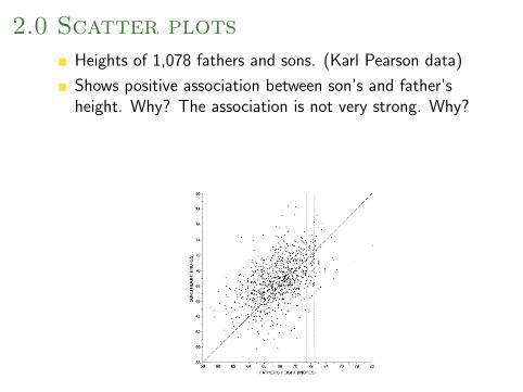
2.0 Scatter plots

Heights of 1,078 fathers and sons. (Karl Pearson data)

Shows positive association between son’s and father’sheight. Why? The association is not very strong. Why?

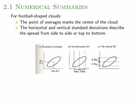
2.1 Numerical Summaries

For football-shaped clouds:

The point of averages marks the center of the cloud.The horizontal and vertical standard deviations describethe spread from side to side or top to bottom.

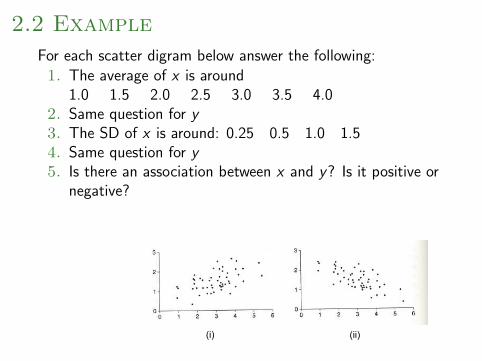
2.2 Example

For each scatter digram below answer the following:1. The average of x is around

1.0 1.5 2.0 2.5 3.0 3.5 4.02. Same question for y3. The SD of x is around: 0.25 0.5 1.0 1.54. Same question for y5. Is there an association between x and y? Is it positive or

negative?

(i) (ii)

3.0 Pearson’s Correlation r

Pearson’s correlation coefficient takes a value between -1and +1.

A positive correlation means the cloud slopes up.

A negative correlation means the cloud slopes down.

A large correlation (close to ± 1) means the pointscluster more tightly around a line.

A small correlation (close to 0) means the cloud isform-less and looks more circular.

3.1 Example

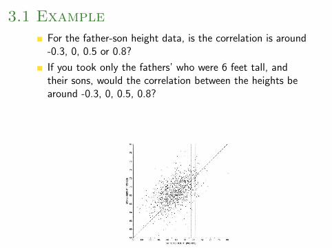
For the father-son height data, is the correlation is around-0.3, 0, 0.5 or 0.8?

If you took only the fathers’ who were 6 feet tall, andtheir sons, would the correlation between the heights bearound -0.3, 0, 0.5, 0.8?

3.2 Calculating r

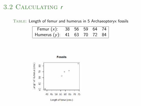
Table: Length of femur and humerus in 5 Archaeopteryx fossils

Femur (x): 38 56 59 64 74Humerus (y): 41 63 70 72 84

3.2 Calculating r

Step 1: Calculate the mean and S.D. for x and y .

Step 2: Calculate standard scores for x and y .

Step 3: Average the products of these standard scores.Divide by n − 1 instead of n.

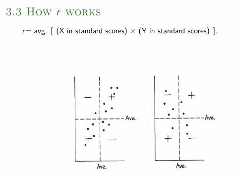
3.3 How r works

r= avg. [ (X in standard scores) × (Y in standard scores) ].

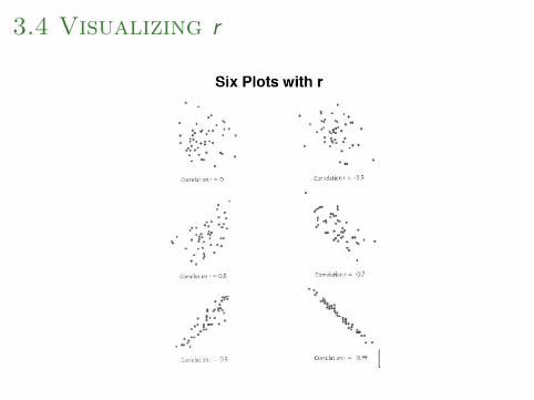
3.4 Visualizing r

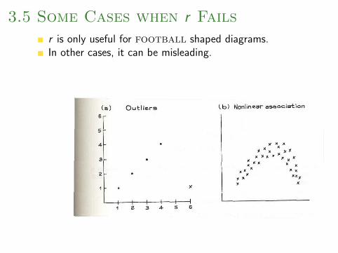
3.5 Some Cases when r Fails

r is only useful for football shaped diagrams.In other cases, it can be misleading.

4.0 Example

The correlation between height and weight among men age18-74 in the U.S. is about 0.40. Say whether each of theseconclusions follows.

Taller men tend to be heavier.

The correlation between weight and height for men age18-74 is also about 0.4.

Heavier men tend to be taller.

If someone eats more and puts on 10 pounds, he is likelyto get somewhat taller.

4.1 Example

For women age 25 and over in the U.S. in 2005, therelationship between age and education level (years ofschooling completed) can be summarized as follows.

average age ≈ 50 years, S.D. ≈ 16 years,average ed. level ≈ 13.2 years, S.D. ≈ 3.0 years, r ≈ -0.2.

True or false: as you get older, you become less educated.Explain.

4.2 Example

A sociologist is studying the relationship between suicide andliteracy in 19th century Italy. He has data for each province,showing the % of literates and the suicide rate in thatprovince. The correlation is 0.6.

1. Provinces with higher literacy rates tend to have highersuicide rates. True or false?

2. Individuals with higher literacy rates tend to commitsuicide more often? True or false?

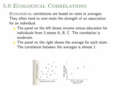
5.0 Ecological Correlations

Ecological correlations are based on rates or averages.They often tend to over-state the strength of an associationfor an individual.

The panel on the left shows income versus education forindividuals from 3 states A, B, C. The correlation ismoderate.The panel on the right shows the average for each state.The correlation between the averages is almost 1.