104
Descriptive Statistics-II Mahmoud Alhussami, MPH, DSc., PhD.

Descriptive Statistics-II
Mahmoud Alhussami, MPH, DSc., PhD.
Shapes of Distribution
A third important property of data – after location and dispersion - is its shape
Distributions of quantitative variables can be described in terms of a number of features, many of which are related to the distributions‟ physical appearance or shape when presented graphically. modality
Symmetry and skewness
Degree of skewness
Kurtosis

Modality
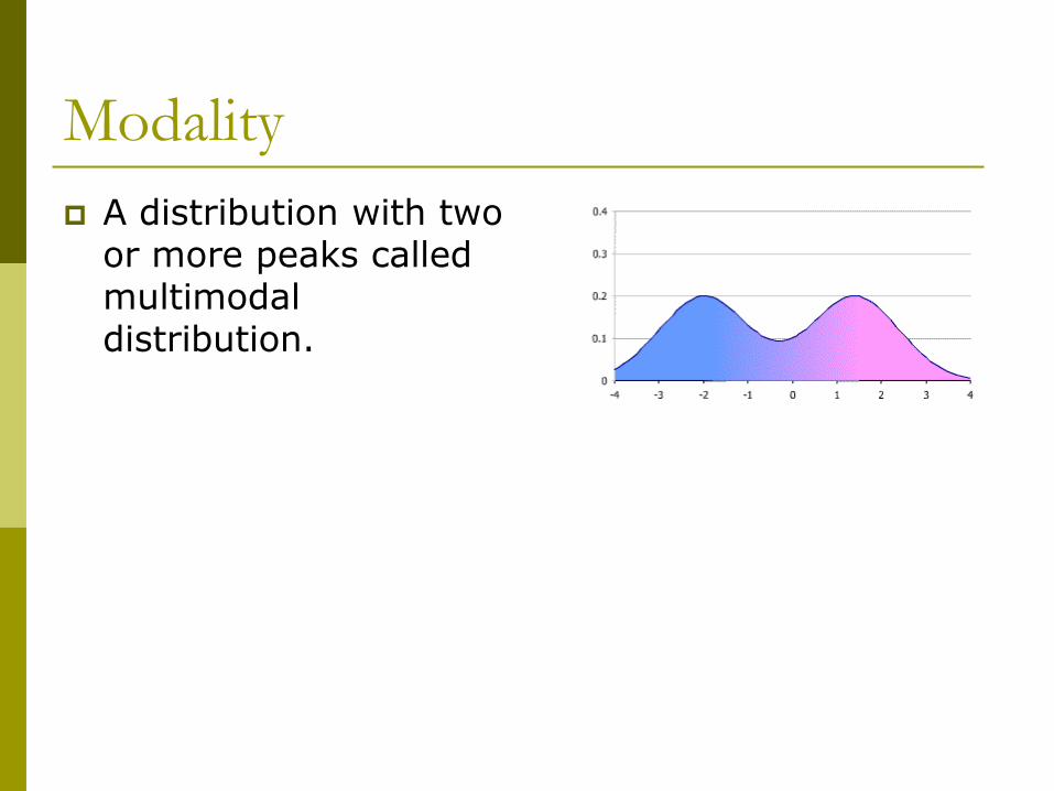
The modality of a distribution concerns how many peaks or high points there are.
A distribution with a single peak, one value a high frequency is a unimodal distribution.
Modality
A distribution with two or more peaks called multimodal distribution.

Symmetry and Skewness
A distribution is symmetric if the distribution could be split down the middle to form two haves that are mirror images of one another.
In asymmetric distributions, the peaks are off center, with a bull of scores clustering at one end, and a tail trailing off at the other end. Such distributions are often describes as skewed. When the longer tail trails off to the right this is a positively
skewed distribution. E.g. annual income.
When the longer tail trails off to the left this is called negatively skewed distribution. E.g. age at death.
Symmetry and Skewness
Shape can be described by degree of asymmetry (i.e., skewness). mean > median positive or right-skewness mean = median symmetric or zero-skewness mean < median negative or left-skewness
Positive skewness can arise when the mean is increased by some unusually high values.
Negative skewness can arise when the mean is decreased by some unusually low values.

Left skewed:
Right skewed:
Symmetric:
7

9 March 2014 8
Shapes of the Distribution
Three common shapes of frequency distributions:
Symmetrical
and bell
shaped
Positively
skewed or
skewed to
the right
Negatively
skewed or
skewed to
the left
A B C

9 March 2014 9
Shapes of the Distribution
Three less common shapes of frequency distributions:
Bimodal Reverse
J-shaped
Uniform
A B C

10
This guy took a VERY long time!
Degree of Skewness
A skewness index can readily be calculated most statistical computer program in conjunction with frequency distributions
The index has a value of 0 for perfectly symmetric distribution.
A positive value if there is a positive skew, and negative value if there is a negative skew.
A skewness index that is more than twice the value of its standard error can be interpreted as a departure from symmetry.

Measures of Skewness or Symmetry
Pearson‟s skewness coefficient
It is nonalgebraic and easily calculated. Also it is useful for quick estimates of symmetry .
It is defined as:
skewness = mean-median/SD
Fisher‟s measure of skewness.
It is based on deviations from the mean to the third power.
Pearson‟s skewness coefficient
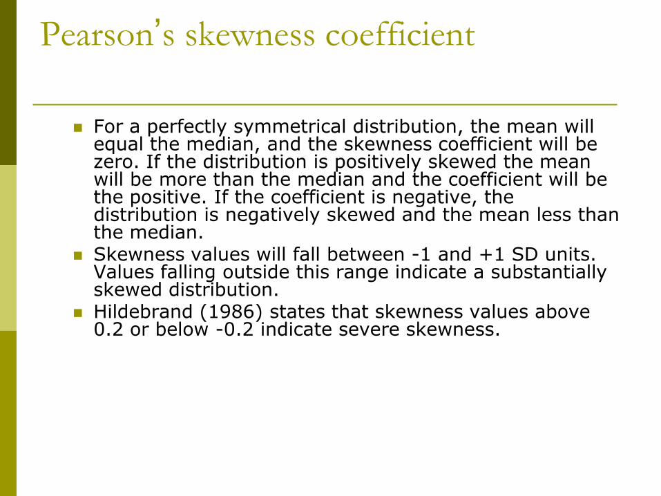
For a perfectly symmetrical distribution, the mean will equal the median, and the skewness coefficient will be zero. If the distribution is positively skewed the mean will be more than the median and the coefficient will be the positive. If the coefficient is negative, the distribution is negatively skewed and the mean less than the median.
Skewness values will fall between -1 and +1 SD units. Values falling outside this range indicate a substantially skewed distribution.
Hildebrand (1986) states that skewness values above 0.2 or below -0.2 indicate severe skewness.
Fisher‟s Measure of Skewness
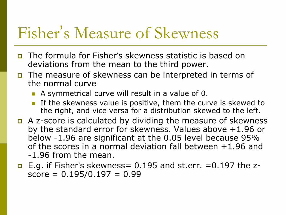
The formula for Fisher‟s skewness statistic is based on deviations from the mean to the third power.
The measure of skewness can be interpreted in terms of the normal curve A symmetrical curve will result in a value of 0.
If the skewness value is positive, them the curve is skewed to the right, and vice versa for a distribution skewed to the left.
A z-score is calculated by dividing the measure of skewness by the standard error for skewness. Values above +1.96 or below -1.96 are significant at the 0.05 level because 95% of the scores in a normal deviation fall between +1.96 and -1.96 from the mean.
E.g. if Fisher‟s skewness= 0.195 and st.err. =0.197 the z-score = 0.195/0.197 = 0.99

Kurtosis
The distribution‟s kurtosis is concerns how
pointed or flat its peak.
Two types:
Leptokurtic distribution (mean thin).
Platykurtic distribution (means flat).

Kurtosis
There is a statistical index of kurtosis that can be
computed when computer programs are instructed to produce a frequency distribution
For kurtosis index, a value of zero indicates a shape that is neither flat nor pointed.
Positive values on the kurtosis statistics indicate greater peakedness, and negative values indicate greater flatness.

Fishers‟ measure of Kurtosis
Fisher‟s measure is based on deviation
from the mean to the fourth power.
A z-score is calculated by dividing the measure of kurtosis by the standard error for kurtosis.

Normal Distribution
Also called belt shaped curve, normal curve, or Gaussian distribution.
A normal distribution is one that is unimodal, symmetric, and not too peaked or flat.
Given its name by the French mathematician Quetelet who, in the early 19th century noted that many human attributes, e.g. height, weight, intelligence appeared to be distributed normally.

9 March 2014 19
Normal Distribution
The normal curve is unimodal and symmetric about its mean ().
In this distribution the mean, median and mode are all identical.
The standard deviation () specifies the amount of dispersion around the mean.
The two parameters and completely define a normal curve.
Also called a Probability density function. The probability is interpreted as "area under the curve.“
The area under the whole curve = 1

Sampling Distribution A sample statistic is often unequal to the value of the
corresponding population parameter because of sampling error.
Sampling error reflects the tendency for statistics to fluctuate from one sample to another.
The amount of sampling error is the difference between the obtained sample value and the population parameter.
Inferential statistics allow researchers to estimate how close to the population value the calculated statistics is likely to be.
The concept of sampling, which are actually probability distributions, is central to estimates of sampling error.

Characteristics of Sampling Distribution
Sampling error= sample mean-population mean. Every sample size has a different sampling distribution of
the mean. Sampling distributions are theoretical, because in practice,
no one draws an infinite number of samples from a population.
Their characteristics can be modeled mathematically and have determined by a formulation known as the central limit theorem.
This theorem stipulates that the mean of the sampling distribution is identical to the population mean.
A consequence of Central Limit Theorem is that if we average measurements of a particular quantity, the distribution of our average tends toward a normal one.
The average sampling error-the mean of the (mean-μ)sample would always equal zero.

Standard Error of the Mean
The standard deviation of a sampling distribution of the mean has a special name: the standard error of the mean (SEM).
The smaller the SEM, the more accurate are the sample means as estimates of the population value.

Central Limit Theorem
describes the characteristics of the "population of the means" which has been created from the means of an infinite number of random population samples of size (N), all of them drawn from a given "parent population".
It predicts that regardless of the distribution of the parent population: The mean of the population of means is always equal to the
mean of the parent population from which the population samples were drawn.
The standard deviation of the population of means is always equal to the standard deviation of the parent population divided by the square root of the sample size (N).
The distribution of means will increasingly approximate a normal distribution as the size N of samples increases.

9 March 2014 24
Standard Normal Variable
It is customary to call a standard normal random variable Z.
The outcomes of the random variable Z are denoted by z.
The table in the coming slide give the area under the curve (probabilities) between the mean and z.
The probabilities in the table refer to the likelihood that a randomly selected value Z is equal to or less than a given value of z and greater than 0 (the mean of the standard normal).

25
Source: Levine et al, Business Statistics, Pearson.

9 March 2014 26
The 68-95-99.7 Rule for the Normal
Distribution 68% of the observations fall within one
standard deviation of the mean
95% of the observations fall within two standard deviations of the mean
99.7% of the observations fall within three standard deviations of the mean
When applied to „real data‟, these
estimates are considered approximate!
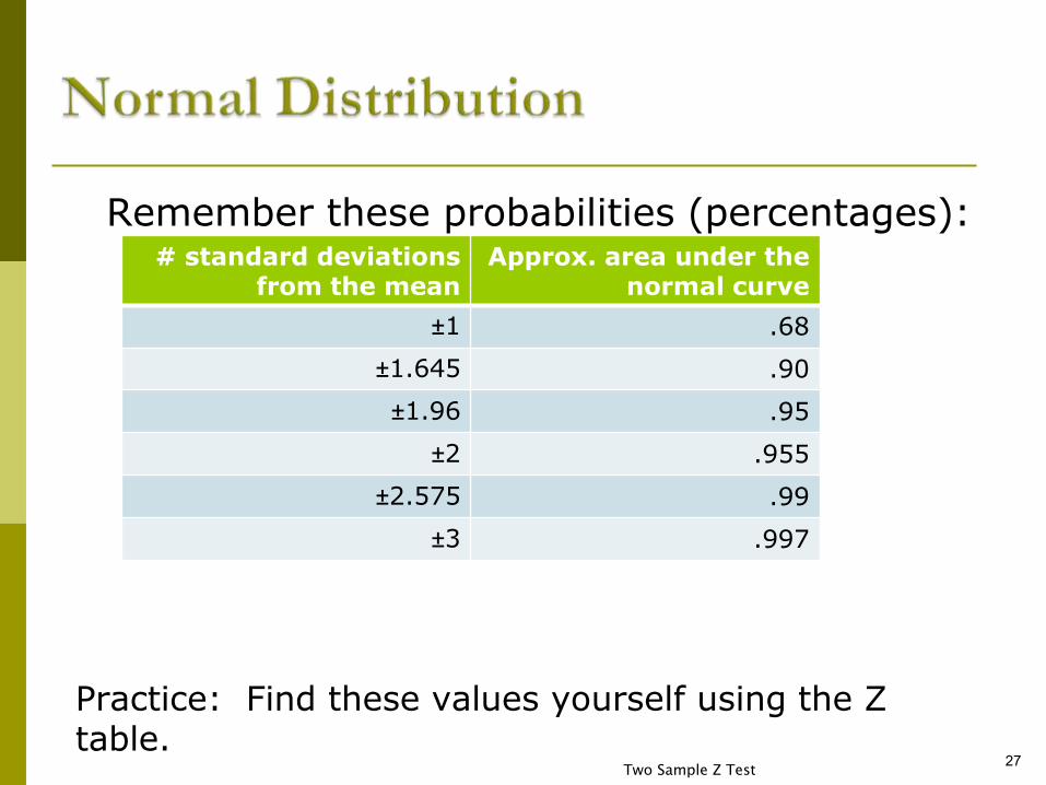
Remember these probabilities (percentages):
Practice: Find these values yourself using the Z table.
Two Sample Z Test27
# standard deviations from the mean
Approx. area under the normal curve
±1 .68
±1.645 .90
±1.96 .95
±2 .955
±2.575 .99
±3 .997

9 March 2014 28
Standard Normal Curve

9 March 2014 29
Standard Normal Distribution
50% of probability in
here–probability=0.5
50% of probability in
here –probability=0.5

9 March 2014 30
Standard Normal Distribution
2.5% of
probability in here
2.5% of probability
in here
95% of
probability
in here
Standard Normal
Distribution with 95% area
marked

9 March 2014 31
Calculating Probabilities
Probability calculations are always concerned with finding the probability that the variable assumes any value in an interval between two specific points a andb.
The probability that a continuous variable assumes the a value between a and b is the area under the graph of the density between a and b.
Normal Distribution 32
If the weight of males is N.D. with μ=150 and σ=10, what is the probability that a randomly selected male will weigh between 140 lbs and
155 lbs?

Solution:
Z = (140 – 150)/ 10 = -1.00 s.d. from mean
Area under the curve = .3413 (from Z table)
Z = (155 – 150) / 10 =+.50 s.d. from mean
Area under the curve = .1915 (from Z table)
Answer: .3413 + .1915 = .5328
33
150 155
X
Z 0.5 -1 0
140

If IQ is ND with a mean of 100 and a S.D. of 10, what percentage of the population will have (a)IQs ranging from 90 to 110? (b)IQs ranging from 80 to 120?Solution: Z = (90 – 100)/10 = -1.00Z = (110 -100)/ 10 = +1.00 Area between 0 and 1.00 in the Z-table is .3413; Area between 0 and -1.00 is also .3413 (Z-distribution is symmetric). Answer to part (a) is .3413 + .3413 = .6826.
34

(b) IQs ranging from 80 to 120?
Solution:
Z = (80 – 100)/10 = -2.00
Z = (120 -100)/ 10 = +2.00
Area between =0 and 2.00 in the Z-table is .4772; Area between 0 and -2.00 is
also .4772 (Z-distribution is symmetric).
Answer is .4772 + .4772 = .9544.
35

Suppose that the average salary of college graduates is N.D. with μ=$40,000 and σ=$10,000.
(a) What proportion of college graduates will earn $24,800 or less?
(b) What proportion of college graduates will earn $53,500 or more?
(c) What proportion of college graduates will earn between $45,000 and $57,000?
(d) Calculate the 80th percentile.
(e) Calculate the 27th percentile.
36

(a) What proportion of college graduates will earn $24,800 or less?
Solution:
Convert the $24,800 to a Z-score: Z = ($24,800 - $40,000)/$10,000 = -1.52.
Always DRAW a picture of the distribution to help you solve these problems.
37

First Find the area between 0 and -1.52 in the Z-table. From the Z table, that area is .4357. Then, the area from -1.52 to - ∞ is .5000 - .4357 = .0643.Answer: 6.43% of college graduates will earn less than $24,800.
38
$24,800 $40,000
-1.52 0
.4357
X
Z

(b) What proportion of college graduates will earn $53,500 or more?Solution: Convert the $53,500 to a Z-score.Z = ($53,500 - $40,000)/$10,000 = +1.35. Find the area between 0 and +1.35 in the Z-table: .4115 is the table value.When you DRAW A PICTURE (above) you see that you need the area in the tail: .5 - .4115 -.0885.Answer: .0885. Thus, 8.85% of college graduates will earn $53,500 or more.
39
$40,000 $53,500
Z0 +1.35
.4115
.0885

(c) What proportion of college graduates will earn between $45,000 and $57,000?
Z = $45,000 – $40,000 / $10,000 = .50Z = $57,000 – $40,000 / $10,000 = 1.70
From the table, we can get the area under the curve between the mean (0) and .5; we can get the area between 0 and 1.7. From the picture we see that neither one is what we need.What do we do here? Subtract the small piece from the big piece to get exactly what we need.Answer: .4554 − .1915 = .2639
40
$40k
Z0 1.7
$45k $57k
.5
.1915

Parts (d) and (e) of this example ask you to compute percentiles. Every Z-score is associated with a percentile. A Z-score of 0 is the 50th percentile. This means that if you take any test that is normally distributed (e.g., the SAT exam), and your Z-score on the test is 0, this means you scored at the 50th percentile. In fact, your score is the mean, median, and mode.
41
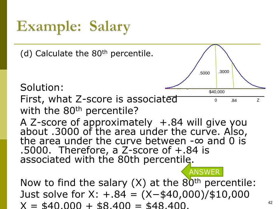
(d) Calculate the 80th percentile.
Solution:First, what Z-score is associated with the 80th percentile? A Z-score of approximately +.84 will give you about .3000 of the area under the curve. Also, the area under the curve between -∞ and 0 is .5000. Therefore, a Z-score of +.84 is associated with the 80th percentile.
Now to find the salary (X) at the 80th percentile: Just solve for X: +.84 = (X−$40,000)/$10,000 X = $40,000 + $8,400 = $48,400.
42
$40,000
Z0 .84
.3000.5000
ANSWER

(e) Calculate the 27th percentile.
Solution: First, what Z-score is associated with the 27th percentile? A Z-score of approximately -.61will give you about .2300 of the area under the curve, with .2700 in the tail. (The area under the curve between 0 and -.61 is .2291 which we are rounding to .2300). Also, the area under the curve between 0 and ∞ is .5000. Therefore, a Z-score of -.61 is associated with the 27th percentile.
Now to find the salary (X) at the 27th percentile: Just solve for X: -0.61 =(X−$40,000)/$10,000 X = $40,000 - $6,100 = $33,900
43
$40,000
Z0-.61
.5000.2300
ANSWER
.2700

9 March 2014 44
Graphical Methods
Frequency Distribution
Histogram
Frequency Polygon
Cumulative Frequency Graph
Pie Chart.

Presenting Data
Table
Condenses data into a form that can make them easier to understand;
Shows many details in summary fashion;
BUT
Since table shows only numbers, it may not be readily understood without comparing it to other values.

Principles of Table Construction
Don‟t try to do too much in a table
Us white space effectively to make table layout pleasing to the eye.
Make sure tables & test refer to each other.
Use some aspect of the table to order & group rows & columns.

Principles of Table Construction
If appropriate, frame table with summary statistics in rows & columns to provide a standard of comparison.
Round numbers in table to one or two decimal places to make them easily understood.
When creating tables for publication in a manuscript, double-space them unless contraindicated by journal.
9 March 2014 48
Frequency Distributions
A useful way to present data when you have a large data set is the formation of a frequency table or frequency distribution.
Frequency – the number of observations
that fall within a certain range of the data.

49
Frequency Table
Age Number of Deaths
<1 564
1-4 86
5-14 127
15-24 490
25-34 66
35-44 806
45-54 1,425
55-64 3,511
65-74 6,932
75-84 10,101
85+ 9825
Total 34,524

Presenting Data
Chart
Visual representation of a frequency distribution that helps to gain insight about what the data mean.
Built with lines, area & text: bar
charts, pie chart

Bar Chart
Simplest form of chart
Used to display nominal or ordinal data
ETHICAL ISSUES SCALE
ITEM 8
ACTING AGAINST YOUR OWN PERSONAL/RELIGIOUS VIEWS
FrequentlySomet imesSeldomNever
PE
RC
EN
T
60
50
40
30
20
10
0
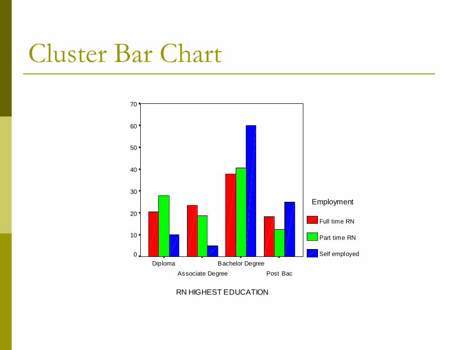
Cluster Bar Chart
RN HIGHEST EDUCATION
Post Bac
Bachelor Degree
Associate Degree
Diploma
PE
RC
EN
T
70
60
50
40
30
20
10
0
Employment
Full time RN
Part time RN
Self employed
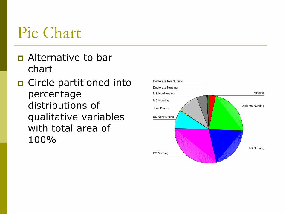
Pie Chart
Alternative to bar chart
Circle partitioned into percentage distributions of qualitative variables with total area of 100%
Doctorate NonNursing
Doctorate Nursing
MS NonNursing
MS Nursing
Juris Doctor
BS NonNursing
BS Nursing
AD Nursing
Diploma-Nursing
Missing

Histogram
Appropriate for interval, ratio and sometimes ordinal data
Similar to bar charts but bars are placed side by side
Often used to represent both frequencies and percentages
Most histograms have from 5 to 20 bars

Histogram
SF-36 VITALITY SCORES
100.0
90.0
80.0
70.0
60.0
50.0
40.0
30.0
20.0
10.0
0.0
FR
EQ
UE
NC
Y
80
60
40
20
0
Std. Dev = 22.17
Mean = 61.6
N = 439.00

9 March 2014 56
Pictures of Data: Histograms
Blood pressure data on a sample of 113 men
Histogram of the Systolic Blood Pressure for 113 men. Each bar
spans a width of 5 mmHg on the horizontal axis. The height of each
bar represents the number of individuals with SBP in that range.
05
10
15
20
Num
ber
of M
en
80 100 120 140 160
Systolic BP (mmHg)

9 March 2014 57
Frequency Polygon
•First place a dot at the
midpoint of the upper base of
each rectangular bar.
•The points are connected with
straight lines.
•At the ends, the points are
connected to the midpoints of
the previous and succeeding
intervals (these intervals have
zero frequency).
Frequency Polygon
0
2
4
6
8
10
12
14
16
18
20
4.5 14.5 24.5 34.5 44.5 54.5 64.5 74.5 84.5
Childrens w eights

Hallmarks of a Good Chart
Simple & easy to read
Placed correctly within text
Use color only when it has a purpose, not solely for decoration
Make sure others can understand chart; try it out on somebody first
Remember: A poor chart is worse than no chart at all.

9 March 2014 59
Coefficient of Correlation
Measure of linear association between 2 continuous variables.
Setting:
two measurements are made for each observation.
Sample consists of pairs of values and you want to determine the association between the variables.

9 March 2014 60
Association Examples
Example 1: Association between a mother‟s
weight and the birth weight of her child
2 measurements: mother‟s weight and baby‟s weight
Both continuous measures
Example 2: Association between a risk factor and a disease
2 measurements: disease status and risk factor status
Both dichotomous measurements

9 March 2014 61
Correlation Analysis
When you have 2 continuous measurements you use correlation analysis to determine the relationship between the variables.
Through correlation analysis you can calculate a number that relates to the strength of the linear association.

9 March 2014 62
Scatter Plots and Association
You can plot the 2 variables in a scatter plot (one of the types of charts in SPSS/Excel).
The pattern of the “dots” in the plot indicate the statistical relationship between the variables (the strength and the direction). Positive relationship – pattern goes from lower left to
upper right.
Negative relationship – pattern goes from upper left to lower right.
The more the dots cluster around a straight line the stronger the linear relationship.

63
Birth Weight Data
x (oz) y(%)
112 63
111 66
107 72
119 52
92 75
80 118
81 120
84 114
118 42
106 72
103 90
94 91
x – birth weight in ounces
y – increase in weight between
70th and 100th days of life,
expressed as a percentage of
birth weight

9 March 2014 64
Pearson Correlation Coefficient
Birth Weight Data
40
50
60
70
80
90
100
110
120
70 80 90 100 110 120 130 140
Birth Weight (in ounces)
Incre
ase i
n B
irth
Weig
ht
(%)

9 March 2014 65
Calculations of Correlation
Coefficient In SPSS:
Go to TOOLS menu and select DATA ANALYSIS.
Highlight CORRELATION and click “ok”
Enter INPUT RANGE (2 columns of data that contain “x” and “y”)
Click “ok” (cells where you want the answer to
be placed.

9 March 2014 66
Pearson Correlation Results
x (oz) y(%)
x (oz) 1
y(%) -0.94629 1
Pearson Correlation Coefficient = -0.946
Interpretation:
- values near 1 indicate strong positive linear relationship
- values near –1 indicate strong negative linear relationship
- values near 0 indicate a weak linear association

9 March 2014 67
CAUTION!!!!
Interpreting the correlation coefficient should be done cautiously!
A result of 0 does not mean there is NO relationship …. It means there is no
linear association.
There may be a perfect non-linear association.

The Uses of Frequency Distributions
Becoming familiar with dataset.
Cleaning the data. Outliers-values that lie outside the normal range of values for
other cases.
Inspecting the data for missing values.
Testing assumptions for statistical tests. Assumption is a condition that is presumed to be true and
when ignored or violated can lead to misleading or invalid results.
When DV is not normally distributed researchers have to choose between three options: Select a statistical test that does not assume a normal distribution.
Ignore the violation of the assumption.
Transform the variable to better approximate a distribution that is normal. Please consult the various data transformation.

The Uses of Frequency Distributions
Obtaining information about sample characteristics.
Directing answering research questions.

Outliers
Are values that are extreme relative to the bulk of scores in the distribution.
They appear to be inconsistent with the rest of the data.
Advantages:
They may indicate characteristics of the population that would not be known in the normal course of analysis.
Disadvantages:
They do not represent the population
Run counter to the objectives of the analysis
Can distort statistical tests.

Sources of Outliers
An error in the recording of the data.
A failure of data collection, such as not following sample criteria (e.g. inadvertently admitting a disoriented patient into a study), a subject not following instructions on a questionnaire, or equipment failure.
An actual extreme value from an unusual subjects.

Missing Data
Any systematic event external to the respondent (such as data entry errors or data collection problems) or action on the part of the respondent (such as refusal to answer) that leads to missing data.
It means that analyses are based on fewer study participants than were in the full study sample. This, in turn, means less statistical power, which can undermine statistical conclusion validity-the degree to which the statistical results are accurate.
Missing data can also affect internal validity-the degree to which inferences about the causal effect of the dependent variable on the dependent variable are warranted, and also affect the external validity-generalizability.
Strategies to avoid Missing Data
Persistent follow-up
Flexibility in scheduling appointments
Paying incentives.
Using well-proven methods to track people who have moved.
Performing a thorough review of completed data forms prior to excusing participants.
Techniques for Handling Missing Data
Deletion techniques. Involve excluding subjects with missing data from statistical calculation.
Imputation techniques. Involve calculating an estimate of each missing value and replacing, or imputing, each value by its respective estimate.
Note: techniques for handling missing data often vary in the degree to which they affect the amount of dispersion around true scores, and the degree of bias in the final results. Therefore, the selection of a data handling technique should be carefully considered.

Deletion Techniques
Deletion methods involve removal of cases or variables with missing data.
Listwise deletion. Also called complete case analysis. It is simply the analysis of those cases for which there are no missing data. It eliminates an entire case when any of its items/variables has a missing data point, whether or not that data point is part of the analysis. It is the default of the SPSS.
Pairwise deletion. Called the available case analysis (unwise deletion). Involves omitting cases from the analysis on a variable-by-variable basis. It eliminates a case only when that case has missing data for variables or items under analysis.

Imputation Techniques
Imputation is the process of estimating missing data based on valid values of other variables or cases in the sample.
The goal of imputation is to use known relationship that can be identified in the valid values of the sample to help estimate the missing data

Types of Imputation Techniques
Using prior knowledge.
Inserting mean values.
Using regression

Prior Knowledge
Involves replacing a missing value with a value based on an educational guess.
It is a reasonable method if the researcher has a good working knowledge of the research domain, the sample is large, and the number of missing values is small.

Mean Replacement
Also called median replacement for skewed distribution.
Involves calculating mean values from a available data on that variable and using them to replace missing values before analysis.
It is a conservative procedure because the distribution mean as a whole does not change and the researcher does not have to guess at missing values.
Mean Replacement
Advantages: Easily implemented and provides all cases with complete
data.
A compromise procedure is to insert a group mean for the missing values.
Disadvantages: It invalidates the variance estimates derived from the
standard variance formulas by understanding the data‟s true variance.
It distorts the actual distribution of values.
It depresses the observed correlation that this variable will have with other variables because all missing data have a single constant value, thus reducing the variance.
Using Regression
Involves using other variables in the dataset as independent variables to develop a regression equation for the variable with missing data serving as the dependent variable.
Cases with complete data are used to generate the regression equation.
The equation is then used to predict missing values for incomplete cases.
More regressions are computed, using the predicted values from the previous regression to develop the next equation, until the predicted values from one step to the next are comparable.
Prediction from the last regression are the ones used to replace missing values.

Using Regression
Advantages: It is more objective than the researcher‟s guess but not
as blind as simply using the overall mean.
Disadvantages: It reinforces the relationships already in the data,
resulting in less generalizability.
The variance of the distribution is reduced because the estimate is probably too close to the mean.
It assumes that the variable with missing data is correlated substantially with missing data is correlated substantially with the other variables in the dataset.
The regression procedure is not constrained in the estimates it makes.

9 March 2014 83
Categorical Data
Data that can be classified as belonging to a distinct number of categories.
Binary – data can be classified into one of 2 possible categories (yes/no, positive/negative)
Ordinal – data that can be classified into categories that have a natural ordering (i.e.. Levels of pain: none, moderate, intense)
Nominal- data can be classified into >2 categories (i.e.. Race: Arab, African, and other)
9 March 2014 84
Proportions
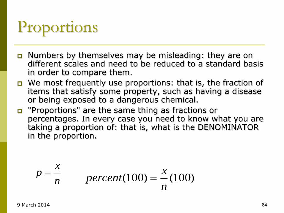
Numbers by themselves may be misleading: they are on different scales and need to be reduced to a standard basis in order to compare them.
We most frequently use proportions: that is, the fraction of items that satisfy some property, such as having a disease or being exposed to a dangerous chemical.
"Proportions" are the same thing as fractions or percentages. In every case you need to know what you are taking a proportion of: that is, what is the DENOMINATOR in the proportion.
n
xp
)100()100(n
xpercent

9 March 2014 85
Proportions and Probabilities
We often interpret proportions as probabilities. If the proportion with a disease is 1/10 then we also say that theprobability of getting the disease is 1/10, or 1 in 10.
Proportions are usually quoted for samples.
Probabilities are almost always quoted for populations.

9 March 2014 86
Workers Example
For the cases:
Proportion of exposure=84/397=0.212 or 21.2%
For the controls:
Proportion of exposure=45/315=0.143 or 14.3%
Smoking Workers Cases Controls
No Yes 11 35
No 50 203
Yes Yes 84 45
No 313 270

9 March 2014 87
Prevalence
Disease Prevalence = the proportion of people with a given disease at a given time.
disease prevalence =
Prevalence is usually quoted as per 100,000 people so the above proportion should be multiplied by 100,000.
Number of diseased persons at a given time
Total number of persons examined at that time

Interpretation
9 March 2014 88
Total
newoldCases
evalence
)(
Pr
Problem of exposure, consequently
Not comparable measurement
Old = duration of the disease
New = speed of the disease
At time t
9 March 2014 89
Screening Tests
Through screening tests people are classified as healthy or as falling into one or more disease categories.
These tests are not 100% accurate and therefore misclassification is unavoidable.
There are 2 proportions that are used to evaluate these types of diagnostic procedures.
9 March 2014 90
Sensitivity and Specificity
Sensitivity and specificity are terms used to describe the effectiveness of screening tests. They describe how good a test is in two ways - finding false positives and finding false negatives
Sensitivity is the Proportion of diseased who screen positive for the disease
Specificity is the Proportion of healthy who screen healthy

Sensitivity and Specificity
Condition Present Condition Absent
……………………………………………………………………………………………
Test Positive True Positive (TP) False Positive (FP)
Test Negative False Negative (FN) True Negative (TN)
……………………………………………………………………………………………
Test Sensitivity (Sn) is defined as the probability that the test is positive when given to a group of patients who have the disease.
Sn= (TP/(TP+FN))x100.
It can be viewed as, 1-the false negative rate.
The Specificity (Sp) of a screening test is defined as the probability that the test will be negative among patients who do not have the disease.
Sp = (TN/(TN+FP))X100.
It can be understood as 1-the false positive rate.

Positive & Negative Predictive Values
The positive predictive value (PPV) of a test is the probability that a patient who tested positive for the disease actually has the disease. PPV = (TP/(TP+FP))X 100.
The negative predictive value (NPV) of a test is the probability that a patent who tested negative for a disease will not have the disease. NPV = (TN/(TN+FN))X100.

The Efficiency
The efficiency (EFF) of a test is the probability that the test result and the diagnosis agree.
It is calculated as:
EFF = ((TP+TN)/(TP+TN+FP+FN)) X 100

9 March 2014 94
Example
A cytological test was undertaken to screen women for cervical cancer.
Sensitivity =?
Specificity = ?
Test Positive Test Negative Total
Actually Positive 154 (TP) 225 (FP) 379
Actually Negative 362 (FN)
516 (TP+FN)
23,362 (TN)
23587(FP+TN)
23,724

9 March 2014 95
Relative Risk
Relative risks are the ratio of risks for two different populations (ratio=a/b).
If the risk (or proportion) of having the outcome is 1/10 in one population and 2/10 in a second population, then the relative risk is: (2/10) / (1/10) = 2.0
A relative risk >1 indicates increased risk for the group in the numerator and a relative risk <1 indicates decreased risk for the group in the numerator.
2 group in incidence disease
1 group in incidence diseaseRisk Relative

9 March 2014 96
Relative Risk
Relative risk – the chance that a member of a group receiving some exposure will develop a disease relative to the chance that a member of an unexposed group will develop the same disease.
Recall: a RR of 1.0 indicates that the probabilities of disease in the exposed and unexposed groups are identical – an association between exposure and disease does not exist.
unexposed) |P(disease
exposed)|P(diseaseRR

Odds Ratio
Odds ratio (OR) is how strongly quantify the presence or absence of property A associated with the presence or absence of property B in a given population. It is a measure of association between an exposure and an outcome.
The OR represents the odds that an outcome will occur given a particular exposure, compared to the odds of the outcome occurring in the absence of that exposure.
The odds ratio is the ratio of the odds of the outcome in the two groups. OR=1 Exposure does not affect odds of outcome
OR>1 Exposure associated with higher odds of outcome
OR<1 Exposure associated with lower odds of outcome

When is it used?
Odds ratios are used to compare the relative odds of the occurrence of the outcome of interest (disease or disorder), given exposure to the variable of interest (health characteristic). The odds ratio can also be used to determine whether a particular exposure is a risk factor for a particular outcome, and to compare the magnitude of various risk factors for that outcome.
Odd‟s Ratio= A/B divided by C/D = AD/BC
9 March 2014 99
Odd‟s Ratio and Relative Risk
Odds ratios are better to use in case-control studies (cases and controls are selected and level of exposure is determined retrospectively)
Relative risks are better for cohort studies (exposed and unexposed subjects are chosen and are followed to determine disease status - prospective)

9 March 2014 100
Odd‟s Ratio and Relative Risk
When we have a two-way classification of exposure and disease we can approximate the relative risk by the odds ratio
Relative Risk=A/(A+B) divided by C/(C+D)
Odd‟s Ratio= A/B divided by C/D = AD/BC
Exposure
Disease
Yes No
Yes A B A+B
No C D C+D

9 March 2014 101
Case Control Study Example
Disease: Pancreatic Cancer
Exposure: Cigarette Smoking
Exposure
Disease
Yes No
Yes 38 81 119
No 2 56 58
9 March 2014 102
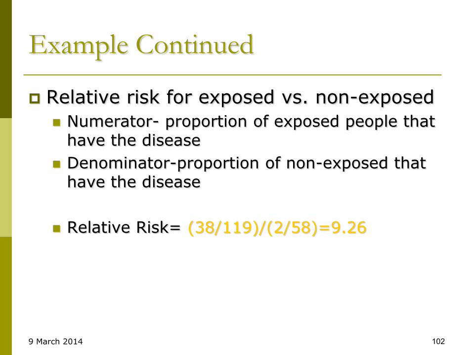
Example Continued
Relative risk for exposed vs. non-exposed
Numerator- proportion of exposed people that have the disease
Denominator-proportion of non-exposed that have the disease
Relative Risk= (38/119)/(2/58)=9.26

9 March 2014 103
Example Continued
Odd‟s Ratio for exposed vs. non-exposed
Numerator- ratio of diseased vs. non-diseased in the exposed group
Denominator- ratio of diseased vs. non-diseased in the non-exposed group
Odd‟s Ratio= (38/81)/(2/56)=(38*56)/(2*81)
=13.14


