Design and Analysis of Algorithms – Chapter 3 1 Brute Force * Dr. Ying Lu [email protected]RAIK 283: Data Structures & RAIK 283: Data Structures & Algorithms Algorithms *slides referred to http://www.aw-bc.com/info/levitin http://www.aw-bc.com/info/levitin September 20, 2012
RAIK 283: Data Structures & RAIK 283: Data Structures & AlgorithmsAlgorithms
*slides referred to http://www.aw-bc.com/info/levitinhttp://www.aw-bc.com/info/levitin
September 20, 2012
Design and Analysis of Algorithms – Chapter 3 2
Brute forceBrute force
A straightforward approach usually based on problem A straightforward approach usually based on problem statement and definitionsstatement and definitions
Many problems in A.I. and operations research require the Many problems in A.I. and operations research require the systematic processing of vertices and edges of graphssystematic processing of vertices and edges of graphs
Graph representations using data Graph representations using data structuresstructures
Adjacency Matrix RepresentationAdjacency Matrix Representation• Let G = (Let G = (VV, , EE), ), nn = | = |VV|, |, mm = | = |EE|, |, VV = { = {vv1, 1, vv2, …, 2, …, vnvn))
• GG can be represented by an can be represented by an nn nn matrix C matrix C
Design and Analysis of Algorithms – Chapter 4 5
Adjacency list representationAdjacency list representation
Design and Analysis of Algorithms – Chapter 4 6
Traversing graphsTraversing graphs
Depth-First Search (DFS) and Breadth-First Depth-First Search (DFS) and Breadth-First Search (BFS)Search (BFS)• Two elementary traversal strategies Two elementary traversal strategies
• Both provide efficient ways to “visit” each vertex and Both provide efficient ways to “visit” each vertex and edge of a graphedge of a graph
• Both work on directed and undirected graphsBoth work on directed and undirected graphs
• They differ in the order of “visiting” verticesThey differ in the order of “visiting” vertices
Design and Analysis of Algorithms – Chapter 4 7
Depth-first searchDepth-first search
Explore graph always moving away from last visited Explore graph always moving away from last visited vertexvertex
Pseudocode for Depth-first-search of graph G=(V,E)Pseudocode for Depth-first-search of graph G=(V,E)
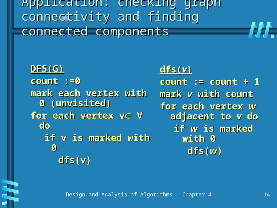
dfs(dfs(vv))count := count + 1count := count + 1mark mark vv with count with countfor each vertex for each vertex ww adjacent to adjacent to
vv dodoif if ww is marked with 0 is marked with 0
dfs(dfs(ww))
DFS(G)DFS(G)count :=0count :=0mark each vertex with 0 mark each vertex with 0
(unvisited)(unvisited)for each vertex vfor each vertex v V doV do
if v is marked with 0 if v is marked with 0 dfs(v)dfs(v)
Design and Analysis of Algorithms – Chapter 4 8
Example – undirected graphExample – undirected graph
Depth-first traversal:Depth-first traversal:
a b
e f
c d
g h
dfs(dfs(vv))count := count + 1count := count + 1mark mark vv with count with countfor each vertex for each vertex ww adjacent to adjacent to
vv dodoif if ww is marked with 0 is marked with 0
dfs(dfs(ww))
Design and Analysis of Algorithms – Chapter 4 9
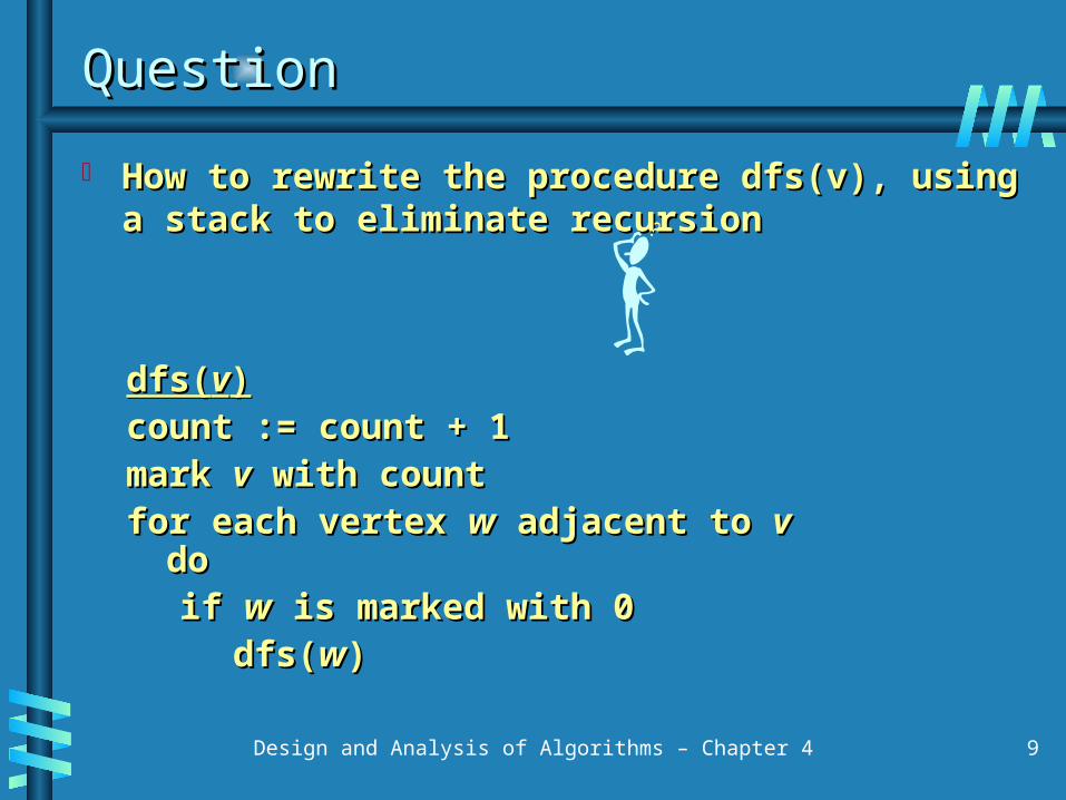
QuestionQuestion
How to rewrite the procedure dfs(v), using a stack to How to rewrite the procedure dfs(v), using a stack to eliminate recursioneliminate recursion
dfs(dfs(vv))count := count + 1count := count + 1mark mark vv with count with countfor each vertex for each vertex ww adjacent to adjacent to vv dodo
if if ww is marked with 0 is marked with 0 dfs(dfs(ww))
Design and Analysis of Algorithms – Chapter 4 10
Non-recursive version of DFS Non-recursive version of DFS algorithmalgorithm
Algorithm dfs(v)s.createStack();s.push(v);count := count + 1mark v with countwhile (!s.isEmpty()) {
let x be the node on the top of the stack s;if (no unvisited nodes are adjacent to x)
s.pop(); // backtrackelse {
select an unvisited node u adjacent to x;s.push(u);count := count + 1mark u with count
}}
Design and Analysis of Algorithms – Chapter 4 11
Time efficiency analysisTime efficiency analysis
DFS can be implemented with graphs represented as:DFS can be implemented with graphs represented as:• Adjacency matrices:Adjacency matrices:
dfs(dfs(vv))count := count + 1count := count + 1mark mark vv with count with countfor each vertex for each vertex ww adjacent to adjacent to
vv dodoif if ww is marked with 0 is marked with 0
dfs(dfs(ww))
DFS(G)DFS(G)count :=0count :=0mark each vertex with 0 mark each vertex with 0
(unvisited)(unvisited)for each vertex vfor each vertex v V doV do
if v is marked with 0 if v is marked with 0 dfs(v)dfs(v)
Design and Analysis of Algorithms – Chapter 4 12
Time efficiency analysisTime efficiency analysis
DFS can be implemented with graphs represented as:DFS can be implemented with graphs represented as:• Adjacency linked lists:Adjacency linked lists:
dfs(dfs(vv))count := count + 1count := count + 1mark mark vv with count with countfor each vertex for each vertex ww adjacent to adjacent to
vv dodoif if ww is marked with 0 is marked with 0
dfs(dfs(ww))
DFS(G)DFS(G)count :=0count :=0mark each vertex with 0 mark each vertex with 0
(unvisited)(unvisited)for each vertex vfor each vertex v V doV do
if v is marked with 0 if v is marked with 0 dfs(v)dfs(v)
Design and Analysis of Algorithms – Chapter 4 13
Time efficiency analysisTime efficiency analysis
DFS can be implemented with graphs represented as:DFS can be implemented with graphs represented as:• Adjacency matrices: Adjacency matrices: ΘΘ((VV22))
dfs(dfs(vv))count := count + 1count := count + 1mark mark vv with count with countfor each vertex for each vertex ww adjacent to adjacent to
vv dodoif if ww is marked with 0 is marked with 0
dfs(dfs(ww))
DFS(G)DFS(G)count :=0count :=0mark each vertex with 0 mark each vertex with 0
(unvisited)(unvisited)for each vertex vfor each vertex v V doV do
if v is marked with 0 if v is marked with 0 dfs(v)dfs(v)
Design and Analysis of Algorithms – Chapter 4 16
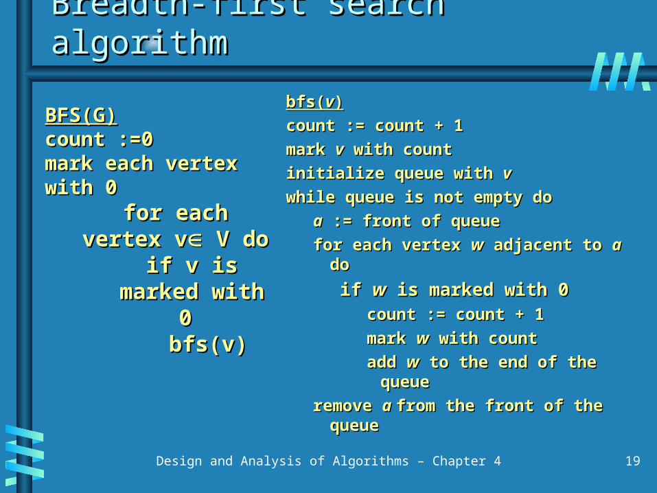
Breadth-first searchBreadth-first search
Explore graph moving across to all the neighbors of last Explore graph moving across to all the neighbors of last visited vertexvisited vertex
Similar to level-by-level tree traversals Similar to level-by-level tree traversals
Applications: same as DFS, but can also find paths from a Applications: same as DFS, but can also find paths from a vertex to all other vertices with the smallest number of vertex to all other vertices with the smallest number of edgesedges
Design and Analysis of Algorithms – Chapter 4 17
Example – undirected graphExample – undirected graph
Breadth-first traversal:Breadth-first traversal:
a b
e f
c d
g h
Design and Analysis of Algorithms – Chapter 4 18
Example – undirected graphExample – undirected graph
Depth-first search could be implemented on a stackDepth-first search could be implemented on a stack How about breadth-first searchHow about breadth-first search
BFS has same efficiency as DFS and can be BFS has same efficiency as DFS and can be implemented with graphs represented as:implemented with graphs represented as:• Adjacency matrices: Adjacency matrices: ΘΘ((VV22))• Adjacency linked lists: Adjacency linked lists: ΘΘ((VV+E)+E)
In-class exerciseIn-class exercise
Exercise 3.2.3 Gadget testingExercise 3.2.3 Gadget testing• A firm wants to determine the highest floor of A firm wants to determine the highest floor of
its n-story headquarters from which a gadget its n-story headquarters from which a gadget can fall with no impact on the gadgetcan fall with no impact on the gadget’’s s functionality. The firm has two identical gadgets functionality. The firm has two identical gadgets to experiment with. Design an algorithm in the to experiment with. Design an algorithm in the best efficiency class you can to solve this best efficiency class you can to solve this problem. problem.
Design and Analysis of Algorithms – Chapter 3 21
Design and Analysis of Algorithms – Chapter 3 22
Brute force polynomial Brute force polynomial evaluationevaluation
Problem: Find the value of polynomial Problem: Find the value of polynomial pp((xx) = ) = aannxxnn + + aann-1-1xxnn-1 -1 +… ++… + a a11xx1 1 + + aa0 0
at a point at a point xx = = xx00
Design and Analysis of Algorithms – Chapter 3 23
Brute force polynomial Brute force polynomial evaluationevaluation
Problem: Find the value of polynomial Problem: Find the value of polynomial pp((xx) = ) = aannxxnn + + aann-1-1xxnn-1 -1 +… ++… + a a11xx1 1 + + aa0 0
at a point at a point xx = = xx00
Algorithm: Algorithm: x := xx := x00
pp := 0.0 := 0.0for for ii := := nn down to 0 do down to 0 do power := 1power := 1 for for jj := 1 to := 1 to ii do do power := power *power := power * x x pp := := p p + + aa[[ii] * power ] * power return return pp
Efficiency:Efficiency:
Design and Analysis of Algorithms – Chapter 3 24
Brute force polynomial Brute force polynomial evaluationevaluation
Problem: Find the value of polynomial Problem: Find the value of polynomial pp((xx) = ) = aannxxnn + + aann-1-1xxnn-1 -1 +… ++… + a a11xx1 1 + + aa0 0
at a point at a point xx = = xx00
Algorithm: Algorithm: x := xx := x00
pp := 0.0 := 0.0for for ii := := nn down to 0 do down to 0 do power := 1power := 1 for for jj := 1 to := 1 to ii do do power := power *power := power * x x pp := := p p + + aa[[ii] * power ] * power return return pp
Efficiency: Efficiency: (n(n22))
Design and Analysis of Algorithms – Chapter 3 25
Brute force polynomial Brute force polynomial evaluationevaluation
Problem: Find the value of polynomial Problem: Find the value of polynomial pp((xx) = ) = aannxxnn + + aann-1-1xxnn-1 -1 +… ++… + a a11xx1 1 + + aa0 0
at a point at a point xx = = xx00
Algorithm: Algorithm: x := xx := x00
pp := 0.0 := 0.0for for ii := := nn down to 0 do down to 0 do power := 1power := 1 for for jj := 1 to := 1 to ii do do power := power *power := power * x x pp := := p p + + aa[[ii] * power ] * power return return pp
Efficiency: Efficiency: (n(n22)) Can we design a linear algorithm for this problemCan we design a linear algorithm for this problem
We can do better by evaluating from right to left: We can do better by evaluating from right to left: pp((xx) = ) = aannxxnn + + aann-1-1xxnn-1 -1 +… +…
++ a a11xx1 1 + + aa0 0 at a point at a point xx = = xx00
Algorithm: Algorithm:
x := xx := x00
pp := := aa[0][0]power := 1power := 1for for ii := 1 to := 1 to nn do do
power := power *power := power * x x pp := := p p + + aa[[ii] * power ] * power
return return pp Efficiency: Efficiency: (n)(n) Can we design a better than linear algorithm for this Can we design a better than linear algorithm for this
problemproblem
Design and Analysis of Algorithms – Chapter 3 28
Brute force closest-pair Brute force closest-pair algorithmalgorithm
Closest pairClosest pair• ProblemProblem: find the closest pair among : find the closest pair among n n points in points in kk-dimensional -dimensional
spacespace
Design and Analysis of Algorithms – Chapter 3 29
Brute force closest-pair Brute force closest-pair algorithmalgorithm
Closest pairClosest pair
• ProblemProblem: find the closest pair among : find the closest pair among n n points in points in kk-dimensional -dimensional spacespace
• AlgorithmAlgorithm: Compute distance between each pair of points and : Compute distance between each pair of points and identify the pair resulting in the shortest distanceidentify the pair resulting in the shortest distance
• What is (or should be) the basic operation of the algorithm?What is (or should be) the basic operation of the algorithm?
Design and Analysis of Algorithms – Chapter 3 30
Brute force closest-pair Brute force closest-pair algorithmalgorithm
Closest pairClosest pair• ProblemProblem: find the closest pair among : find the closest pair among n n points in points in kk-dimensional -dimensional
spacespace• AlgorithmAlgorithm: Compute distance between each pair of points : Compute distance between each pair of points and and
identify the pair resulting in the shortest distanceidentify the pair resulting in the shortest distance
Brute force closest-pair Brute force closest-pair algorithmalgorithm
Closest pairClosest pair• ProblemProblem: : find the closest pair among find the closest pair among n n points in points in kk-dimensional space-dimensional space
• AlgorithmAlgorithm: Compute distance between each pair of points : Compute distance between each pair of points and and identify the pair resulting in the shortest distanceidentify the pair resulting in the shortest distance
• Basic operation:Basic operation:
• How many different pairs of points?How many different pairs of points?
k
iii
k
iii
yxd
yxd
1
22
1
2
)(
)(
Principle of counting: Product Principle of counting: Product RuleRule
The Product RuleThe Product Rule• Suppose that a procedure can be broken down into a sequence of Suppose that a procedure can be broken down into a sequence of
two tasks. If there are ntwo tasks. If there are n11 ways to do the first task and for each of ways to do the first task and for each of
these ways of doing the first task, there are nthese ways of doing the first task, there are n22 ways to do the second ways to do the second
task, then there are ntask, then there are n11nn22 ways to do the procedure. ways to do the procedure.
Design and Analysis of Algorithms – Chapter 3 32
Principle of counting: Product Principle of counting: Product RuleRule
The Product RuleThe Product Rule• Suppose that a procedure can be broken down into a sequence of Suppose that a procedure can be broken down into a sequence of
two tasks. If there are ntwo tasks. If there are n11 ways to do the first task and for each of ways to do the first task and for each of
these ways of doing the first task, there are nthese ways of doing the first task, there are n22 ways to do the second ways to do the second
task, then there are ntask, then there are n11nn22 ways to do the procedure. ways to do the procedure.
CalculationCalculation• Applying the product rule, there are n*(n-1) pairs among n points Applying the product rule, there are n*(n-1) pairs among n points
• Considering (a, b) and (b, a) as the same, we divide the above Considering (a, b) and (b, a) as the same, we divide the above number by 2 and thus, there are n*(n-1)/2 different pairs of pointsnumber by 2 and thus, there are n*(n-1)/2 different pairs of points
Design and Analysis of Algorithms – Chapter 3 33
Design and Analysis of Algorithms – Chapter 3 34
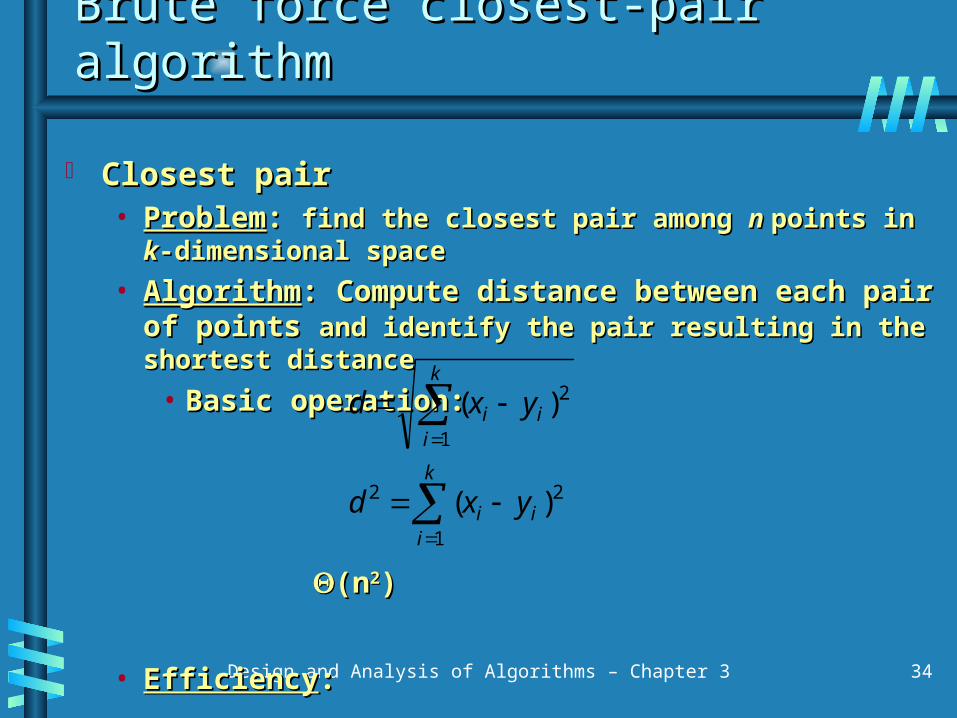
Brute force closest-pair Brute force closest-pair algorithmalgorithm
Closest pairClosest pair• ProblemProblem: : find the closest pair among find the closest pair among n n points in points in kk-dimensional space-dimensional space
• AlgorithmAlgorithm: Compute distance between each pair of points : Compute distance between each pair of points and and identify the pair resulting in the shortest distanceidentify the pair resulting in the shortest distance
• Basic operation:Basic operation:
• EfficiencyEfficiency: :
k
iii
k
iii
yxd
yxd
1
22
1
2
)(
)(
(n(n22))
Design and Analysis of Algorithms – Chapter 3 35
In-class exerciseIn-class exercise
Can you design a faster algorithm than the one based on Can you design a faster algorithm than the one based on the brute-force strategy to solve the closest-pair problem the brute-force strategy to solve the closest-pair problem for n points xfor n points x11, x, x22, … , x, … , xnn on the real line? on the real line?
What is the time efficiency of your algorithm? What is the time efficiency of your algorithm?
Design and Analysis of Algorithms – Chapter 3 36
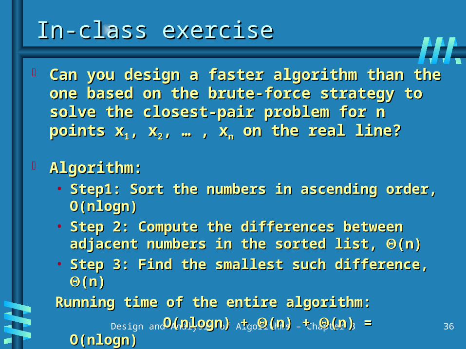
In-class exerciseIn-class exercise
Can you design a faster algorithm than the one based on Can you design a faster algorithm than the one based on the brute-force strategy to solve the closest-pair problem the brute-force strategy to solve the closest-pair problem for n points xfor n points x11, x, x22, … , x, … , xnn on the real line? on the real line?
Algorithm: Algorithm: • Step1: Sort the numbers in ascending order, O(nlogn)Step1: Sort the numbers in ascending order, O(nlogn)
• Step 2: Compute the differences between adjacent numbers in Step 2: Compute the differences between adjacent numbers in the sorted list, the sorted list, (n)(n)
• Step 3: Find the smallest such difference, Step 3: Find the smallest such difference, (n)(n)
Running time of the entire algorithm: Running time of the entire algorithm:
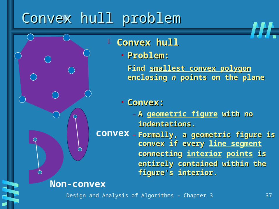
Find Find smallest convex polygonsmallest convex polygon enclosing enclosing nn points on the plane points on the plane
• Convex:Convex:– A A geometric figure with no with no
indentations. indentations. – Formally, a geometric figure is Formally, a geometric figure is
convex if every convex if every line segment connecting connecting interior points is entirely is entirely contained within the figure's interior.contained within the figure's interior.
Computer visualization, ray tracingComputer visualization, ray tracing• (e.g. video games, replacement of bounding boxes)(e.g. video games, replacement of bounding boxes)
Path findingPath finding• (e.g. embedded AI of Mars mission rovers)(e.g. embedded AI of Mars mission rovers)
Geographical Information Systems (GIS)Geographical Information Systems (GIS)• (e.g. computing accessibility maps)(e.g. computing accessibility maps)
Visual pattern matchingVisual pattern matching• (e.g. detecting car license plates)(e.g. detecting car license plates)
Verification methodsVerification methods• (e.g. bounding of Number Decision Diagrams)(e.g. bounding of Number Decision Diagrams)
*slide refer to *slide refer to http://www.montefiore.ulg.ac.be/~briquet/algo3-chull-20070206.pdfhttp://www.montefiore.ulg.ac.be/~briquet/algo3-chull-20070206.pdf
Design and Analysis of Algorithms – Chapter 3 39
Design and Analysis of Algorithms – Chapter 3 40
Convex hull brute force Convex hull brute force algorithmalgorithm
Extreme pointsExtreme points of the of the convex polygonconvex polygon• Consider all the points in the Consider all the points in the
polygon as a set. An polygon as a set. An extreme extreme pointpoint is a point of the set that is a point of the set that is not a middle point of any is not a middle point of any line segment with end points line segment with end points in the set. in the set.
p9
p2
p8
p6
p5
p4
p11
p1
p7p3
p10
Design and Analysis of Algorithms – Chapter 3 41
Convex hull brute force Convex hull brute force algorithmalgorithm
Extreme pointsExtreme points of the of the convex polygonconvex polygon• Consider all the points in the Consider all the points in the
polygon as a set. An polygon as a set. An extreme extreme pointpoint is a point of the set that is a point of the set that is not a middle point of any is not a middle point of any line segment with end points line segment with end points in the set. in the set.
p9
p2
p8
p6
p5
p4
p11
p1
p7p3
p10
Which pairs of extreme points need to be connected Which pairs of extreme points need to be connected to form the boundary of the convex hull?to form the boundary of the convex hull?
Design and Analysis of Algorithms – Chapter 3 42
Convex hull brute force Convex hull brute force algorithmalgorithm
A line segment connecting two points PA line segment connecting two points Pii and P and Pj j of a of a
set of n points is a part of its convex hull’s set of n points is a part of its convex hull’s boundary if and only if all the other points of the boundary if and only if all the other points of the set lies on the same side of the straight line through set lies on the same side of the straight line through these two points.these two points.
Design and Analysis of Algorithms – Chapter 3 43
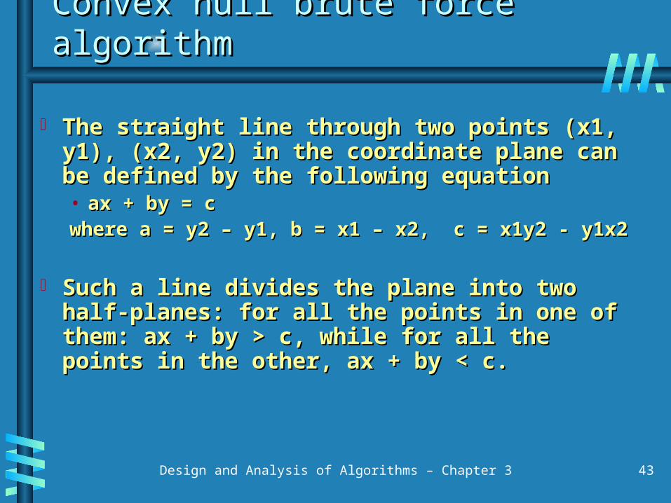
Convex hull brute force Convex hull brute force algorithmalgorithm
The straight line through two points (x1, y1), (x2, The straight line through two points (x1, y1), (x2, y2) in the coordinate plane can be defined by the y2) in the coordinate plane can be defined by the following equationfollowing equation• ax + by = cax + by = cwhere a = y2 – y1, b = x1 – x2, c = x1y2 - y1x2 where a = y2 – y1, b = x1 – x2, c = x1y2 - y1x2
Such a line divides the plane into two half-planes: Such a line divides the plane into two half-planes: for all the points in one of them: ax + by > c, while for all the points in one of them: ax + by > c, while for all the points in the other, ax + by < c. for all the points in the other, ax + by < c.
Design and Analysis of Algorithms – Chapter 3 44
Convex hull brute force Convex hull brute force algorithmalgorithm
AlgorithmAlgorithm: For each pair of points : For each pair of points pp11 and and pp22
determine whether all other points lie to the same determine whether all other points lie to the same side of the straight line through side of the straight line through pp11 and and pp2,2, i.e. whether i.e. whether
ax+by-c all have the same signax+by-c all have the same sign
EfficiencyEfficiency: :
Design and Analysis of Algorithms – Chapter 3 45
Convex hull brute force Convex hull brute force algorithmalgorithm
AlgorithmAlgorithm: For each pair of points : For each pair of points pp11 and and pp22
determine whether all other points lie to the same determine whether all other points lie to the same side of the straight line through side of the straight line through pp11 and and pp2,2, i.e. i.e.
whether ax+by-c all have the same signwhether ax+by-c all have the same sign
A brute force solution to a problem involving A brute force solution to a problem involving search for an element with a special property, search for an element with a special property, usually among combinatorial objects such as a usually among combinatorial objects such as a permutations, combinations, or subsets of a set.permutations, combinations, or subsets of a set.
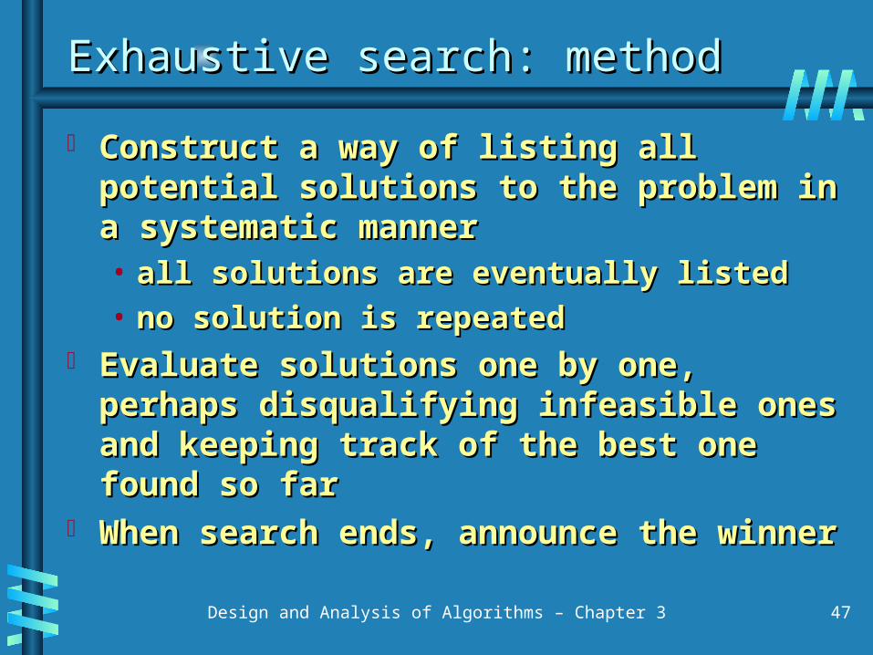
Construct a way of listing all potential solutions to Construct a way of listing all potential solutions to the problem in a systematic mannerthe problem in a systematic manner• all solutions are eventually listedall solutions are eventually listed
• no solution is repeatedno solution is repeated Evaluate solutions one by one, perhaps Evaluate solutions one by one, perhaps
disqualifying infeasible ones and keeping track of disqualifying infeasible ones and keeping track of the best one found so farthe best one found so far
When search ends, announce the winnerWhen search ends, announce the winner
Design and Analysis of Algorithms – Chapter 3 48
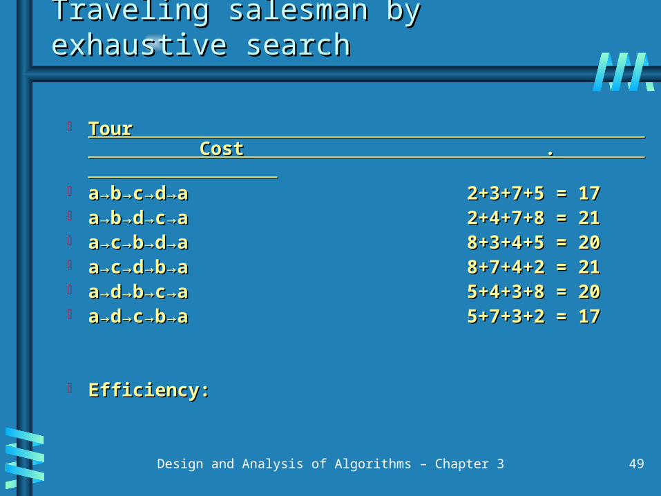
Example 1: Traveling salesman Example 1: Traveling salesman problemproblem
Given Given nn cities with known distances between each cities with known distances between each pair, find the shortest tour that passes through all pair, find the shortest tour that passes through all the cities exactly once before returning to the the cities exactly once before returning to the starting city.starting city.
Alternatively: Find shortest Alternatively: Find shortest Hamiltonian circuitHamiltonian circuit in in a weighted connected graph. a weighted connected graph.
Example:Example:a b
c d
8
2
7
5 34
Design and Analysis of Algorithms – Chapter 3 49
Traveling salesman by exhaustive Traveling salesman by exhaustive searchsearch
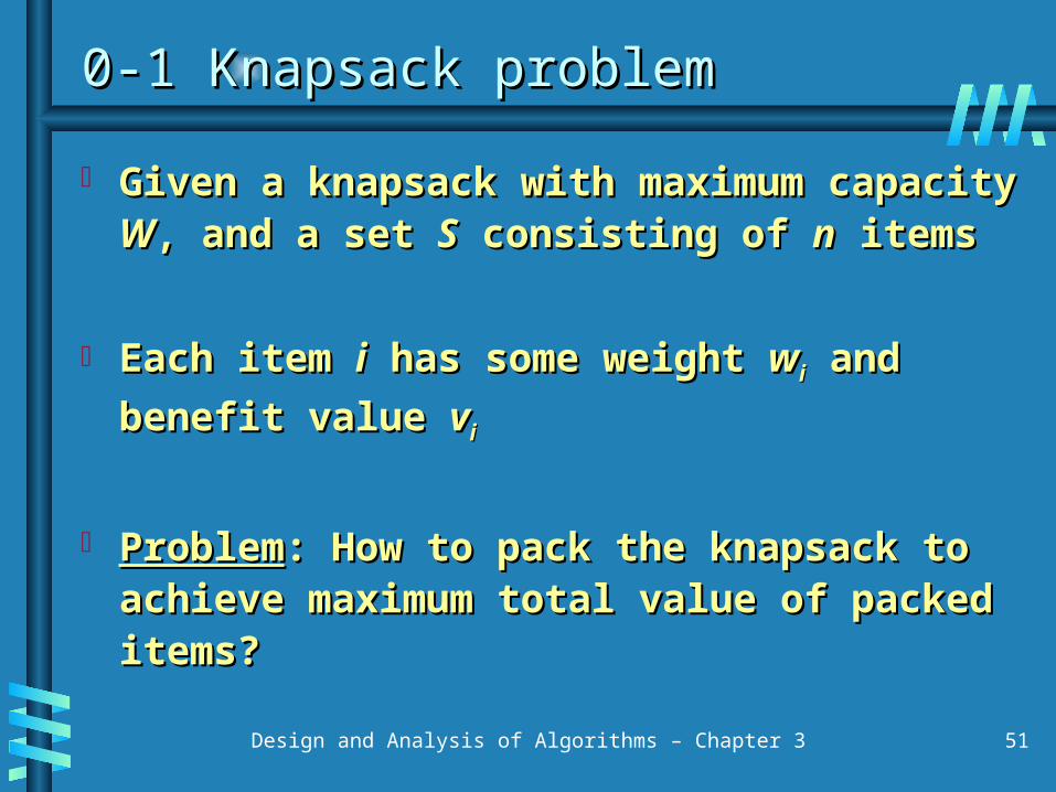
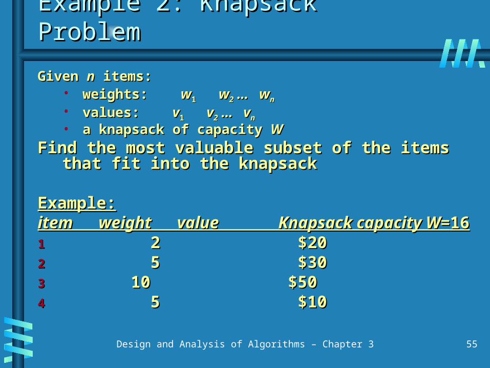
Given a knapsack with maximum capacity Given a knapsack with maximum capacity WW, and , and a set a set SS consisting of consisting of nn items items
Each item Each item ii has some weight has some weight wwii and benefit value and benefit value vvii
ProblemProblem: How to pack the knapsack to achieve : How to pack the knapsack to achieve maximum total value of packed items?maximum total value of packed items?
0-1 Knapsack problem0-1 Knapsack problem
Design and Analysis of Algorithms – Chapter 3 52
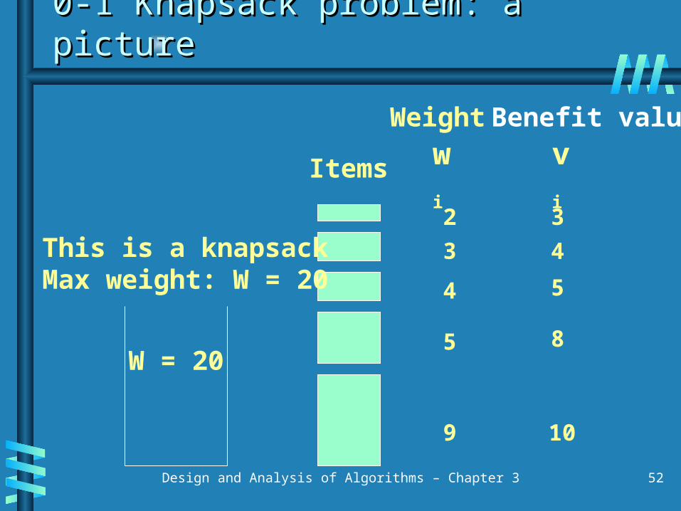
W = 20
wi vi
109
85
54
43
32
Weight Benefit value
This is a knapsackMax weight: W = 20
Items
0-1 Knapsack problem: a 0-1 Knapsack problem: a picturepicture
Design and Analysis of Algorithms – Chapter 3 53
Problem, in other words, is to findProblem, in other words, is to find
Ti
iTi
i Wwv subject to max
0-1 Knapsack problem0-1 Knapsack problem
The problem is called a “The problem is called a “0-10-1” problem, ” problem, because each item must be entirely accepted or because each item must be entirely accepted or rejected.rejected.
In the “In the “Fractional Knapsack ProblemFractional Knapsack Problem,” we can ,” we can take fractions of items. take fractions of items.
Design and Analysis of Algorithms – Chapter 3 54
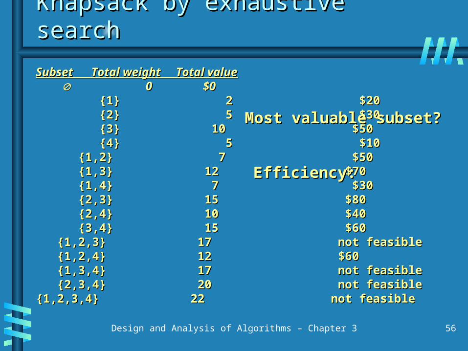
Let’s first solve this problem with a Let’s first solve this problem with a straightforward algorithmstraightforward algorithm
We go through all combinations (subsets) and We go through all combinations (subsets) and find the one with maximum value and with find the one with maximum value and with total weight less or equal to total weight less or equal to WW
• yields reasonable algorithms for some important problemsyields reasonable algorithms for some important problems– sorting; matrix multiplication; closest-pair; convex-hullsorting; matrix multiplication; closest-pair; convex-hull
• yields standard algorithms for simple computational tasks yields standard algorithms for simple computational tasks and graph traversal problemsand graph traversal problems
Design and Analysis of Algorithms – Chapter 3 59
Brute force strengths and Brute force strengths and weaknessesweaknesses
• some brute force algorithms unacceptably slow some brute force algorithms unacceptably slow – e.g., the recursive algorithm for computing Fibonacci numberse.g., the recursive algorithm for computing Fibonacci numbers
• not as constructive/creative as some other design techniquesnot as constructive/creative as some other design techniques