42
Design and analysis of clinical trials MULTIPLE COMPARISONS
| Date post: | 17-Dec-2015 |
| Category: |
Documents |
| Upload: | dylan-elwin-lewis |
| View: | 217 times |
| Download: | 0 times |
Design and analysis of clinical trials
MULTIPLE COMPARISONS
Set area descriptor | Sub level 1
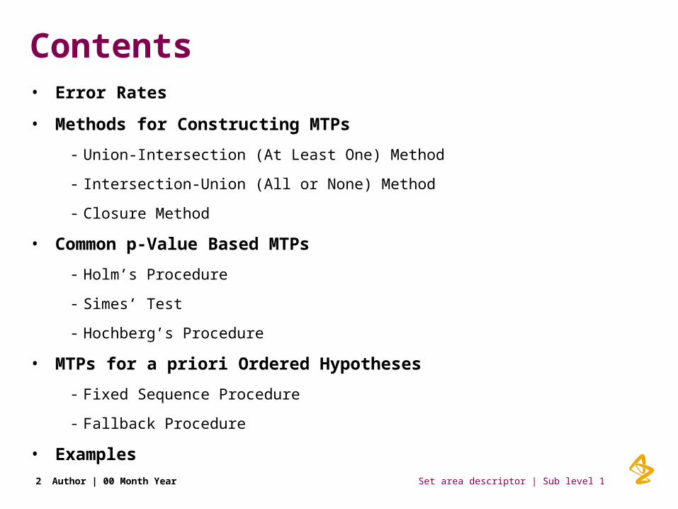
Contents• Error Rates
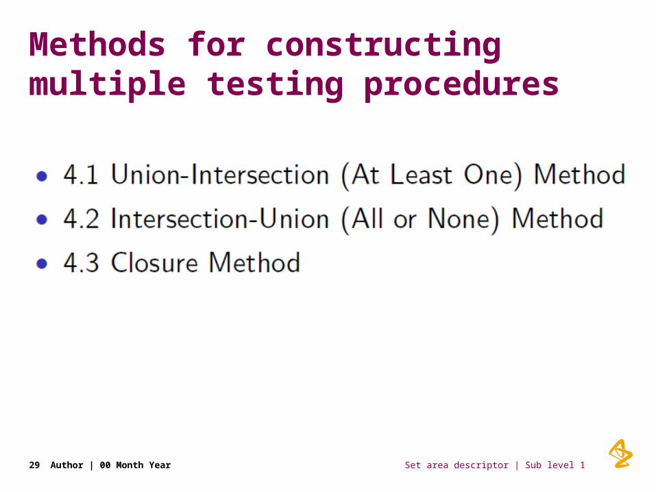
• Methods for Constructing MTPs
- Union-Intersection (At Least One) Method
- Intersection-Union (All or None) Method
- Closure Method
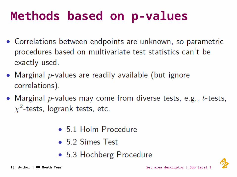
• Common p-Value Based MTPs
- Holm’s Procedure
- Simes’ Test
- Hochberg’s Procedure
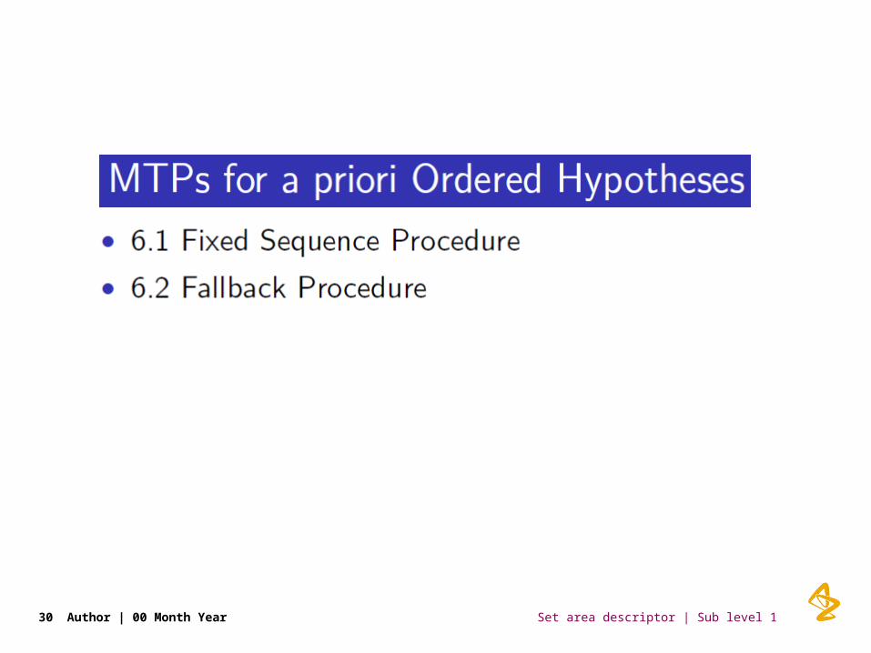
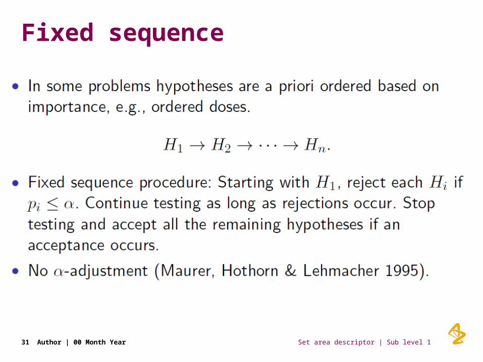
• MTPs for a priori Ordered Hypotheses
- Fixed Sequence Procedure
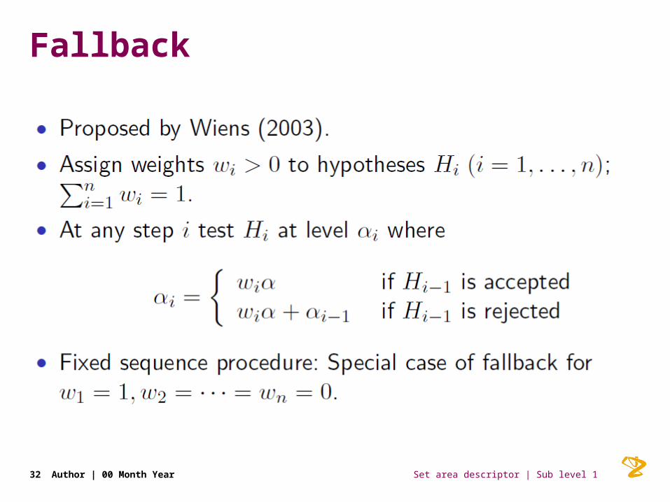
- Fallback Procedure
• Examples2 Author | 00 Month Year
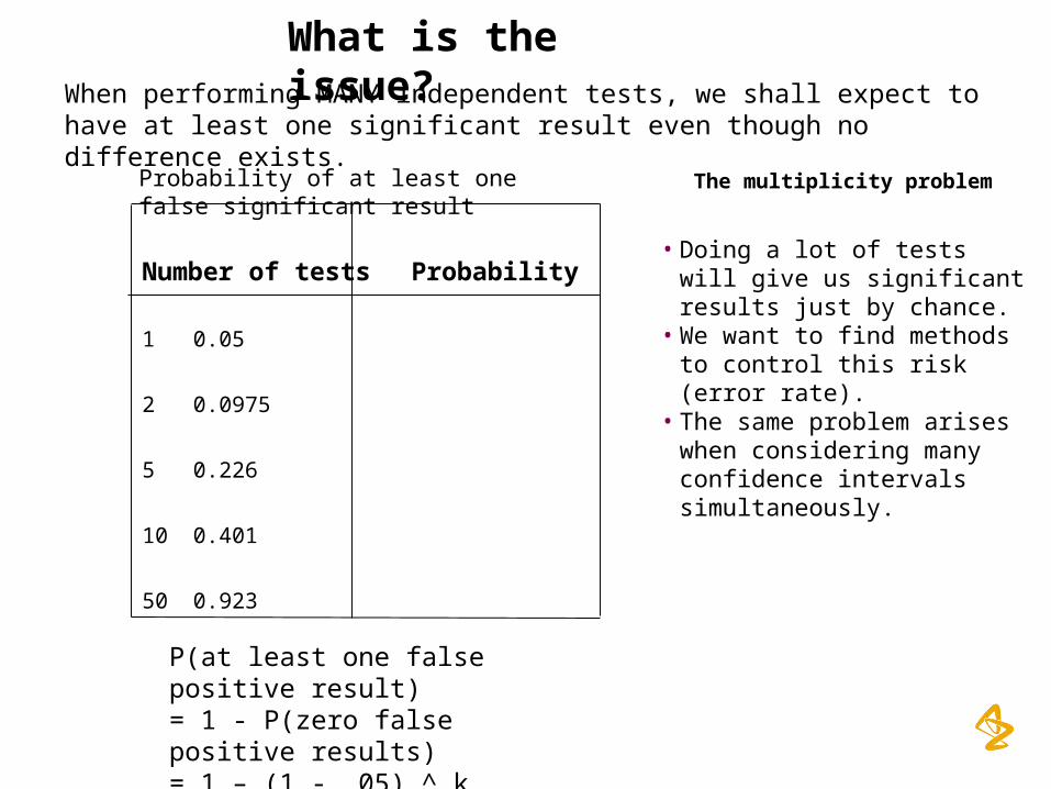
When performing MANY independent tests, we shall expect to have at least one significant result even though no difference exists.
Number of tests Probability
1 0.05
2 0.0975
5 0.226
10 0.401
50 0.923
P(at least one false positive result) = 1 - P(zero false positive results)= 1 – (1 - .05) ^ k
Probability of at least one false significant result
• Doing a lot of tests will give us significant results just by chance.
• We want to find methods to control this risk (error rate).
• The same problem arises when considering many confidence intervals simultaneously.
The multiplicity problem
What is the issue?
Set area descriptor | Sub level 1
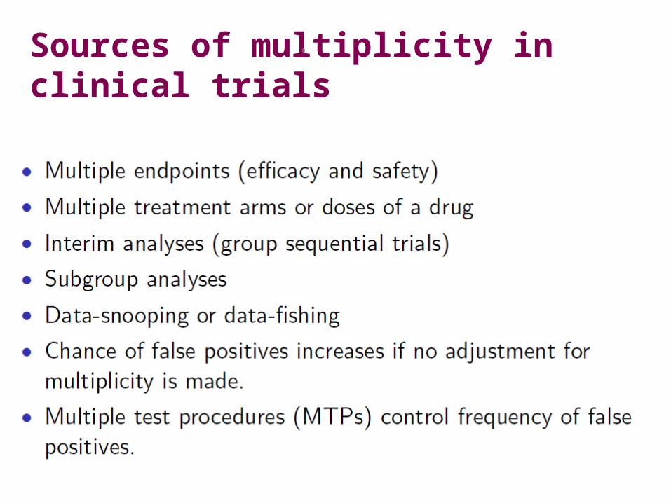
Sources of multiplicity in clinical trials
4 Author | 00 Month Year
8
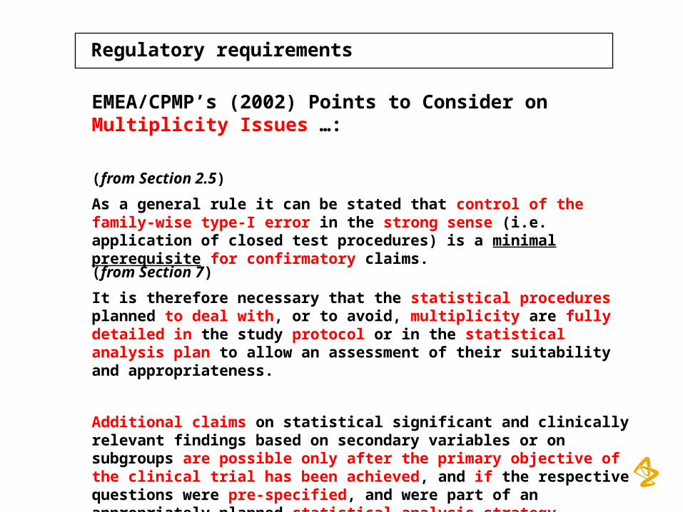
Regulatory requirements
EMEA/CPMP’s (2002) Points to Consider on Multiplicity Issues …:
(from Section 2.5)
As a general rule it can be stated that control of the family-wise type-I error in the strong sense (i.e. application of closed test procedures) is a minimal prerequisite for confirmatory claims.
(from Section 7)
It is therefore necessary that the statistical procedures planned to deal with, or to avoid, multiplicity are fully detailed in the study protocol or in the statistical analysis plan to allow an assessment of their suitability and appropriateness.
Additional claims on statistical significant and clinically relevant findings based on secondary variables or on subgroups are possible only after the primary objective of the clinical trial has been achieved, and if the respective questions were pre-specified, and were part of an appropriately planned statistical analysis strategy
General rulesA. Multiple treatments
• Arrange the treatment comparisons in order of importance• Decide which comparisons should belong to the confirmatory
analysis• Decide a way to control the error of false significances for
these comparisons

General rulesB. Multiple variables
• Find out which variables are needed to answer the primary objective of the study
• Look for possibilities to combine the variables, e.g. composite endpoints, global measures (QoL, AUC etc.)
• Decide a way to control the error of false significances for these variables
General rulesC. Multiple time points
• Find out which time points are the most relevant for the treatment comparison
• If no single time point is most important, look for possibilities to combine the time points, e.g. average over time (AUC etc.)
• Decide a way to control the error of false significances if more than one important time point
General rulesD. Interim analyses
• Decide if the study should stop for safety and/or efficacy reasons• Decide the number of interim analyses• To control the error of a false significance (stopping the study), decide how to
spend the total significance level on the interim and final analysis
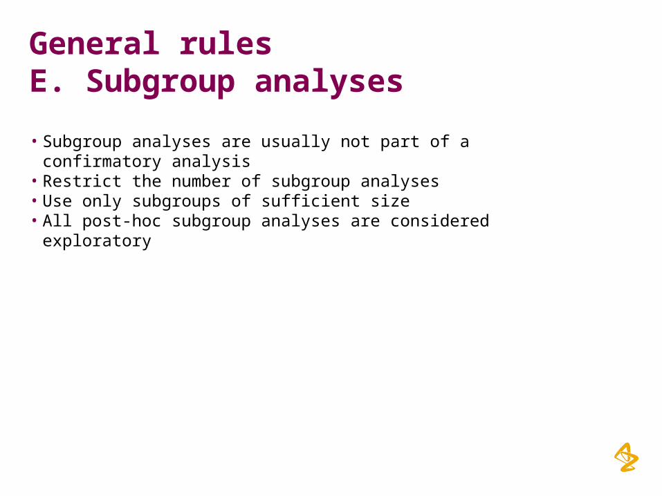
General rulesE. Subgroup analyses
• Subgroup analyses are usually not part of a confirmatory analysis
• Restrict the number of subgroup analyses• Use only subgroups of sufficient size• All post-hoc subgroup analyses are considered exploratory
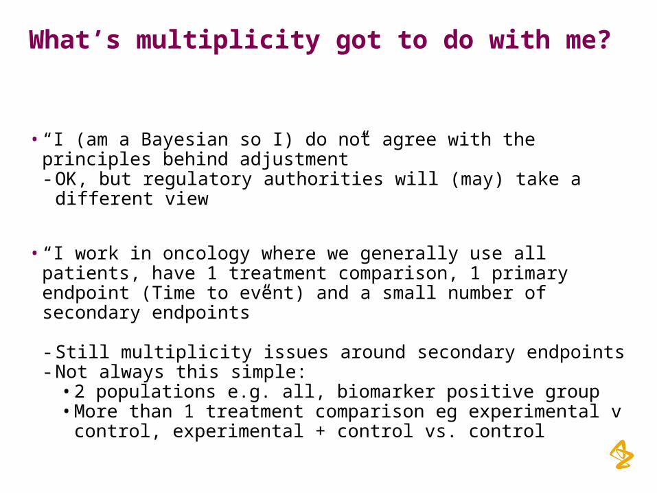
What’s multiplicity got to do with me?
• “I (am a Bayesian so I) do not agree with the principles behind adjustment”- OK, but regulatory authorities will (may) take a different view
• “I work in oncology where we generally use all patients, have 1 treatment comparison, 1 primary endpoint (Time to event) and a small number of secondary endpoints”
- Still multiplicity issues around secondary endpoints- Not always this simple:
• 2 populations e.g. all, biomarker positive group• More than 1 treatment comparison eg experimental v control,
experimental + control vs. control
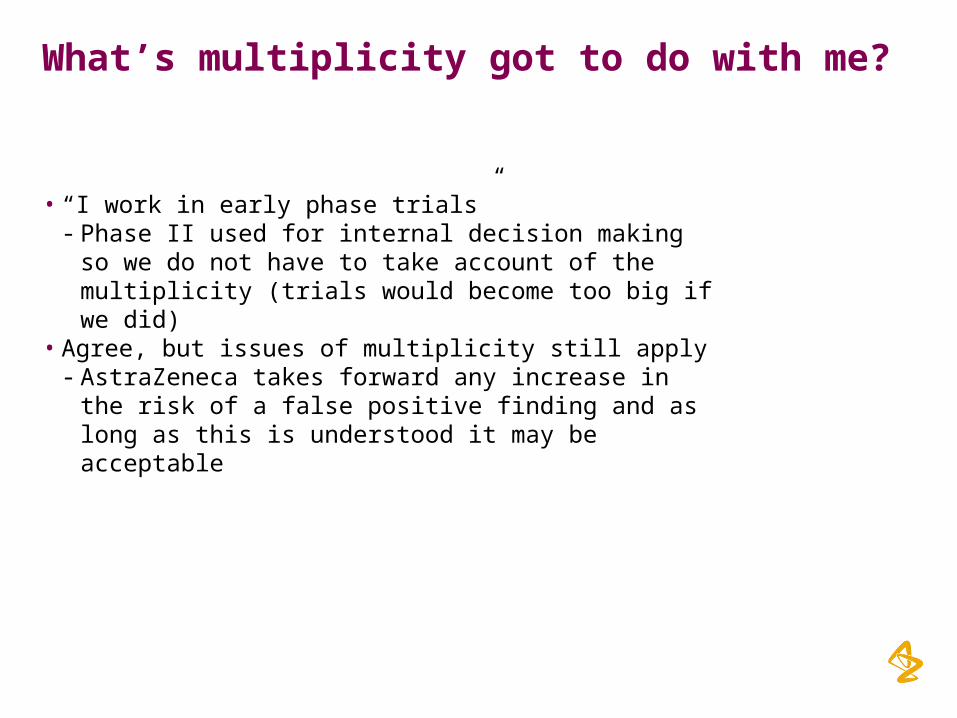
What’s multiplicity got to do with me?
• “I work in early phase trials”- Phase II used for internal decision making so we do not have
to take account of the multiplicity (trials would become too big if we did)
• Agree, but issues of multiplicity still apply- AstraZeneca takes forward any increase in the risk of a false
positive finding and as long as this is understood it may be acceptable
Set area descriptor | Sub level 1
Methods based on p-values
13 Author | 00 Month Year

Bonferroni
• N different null hypotheses H1, … HN
• Calculate corresponding p-values p1, … pN
• Reject Hk if and only if pk < a/N
Variation: The limits may be unequal as long as they sum up to aConservative
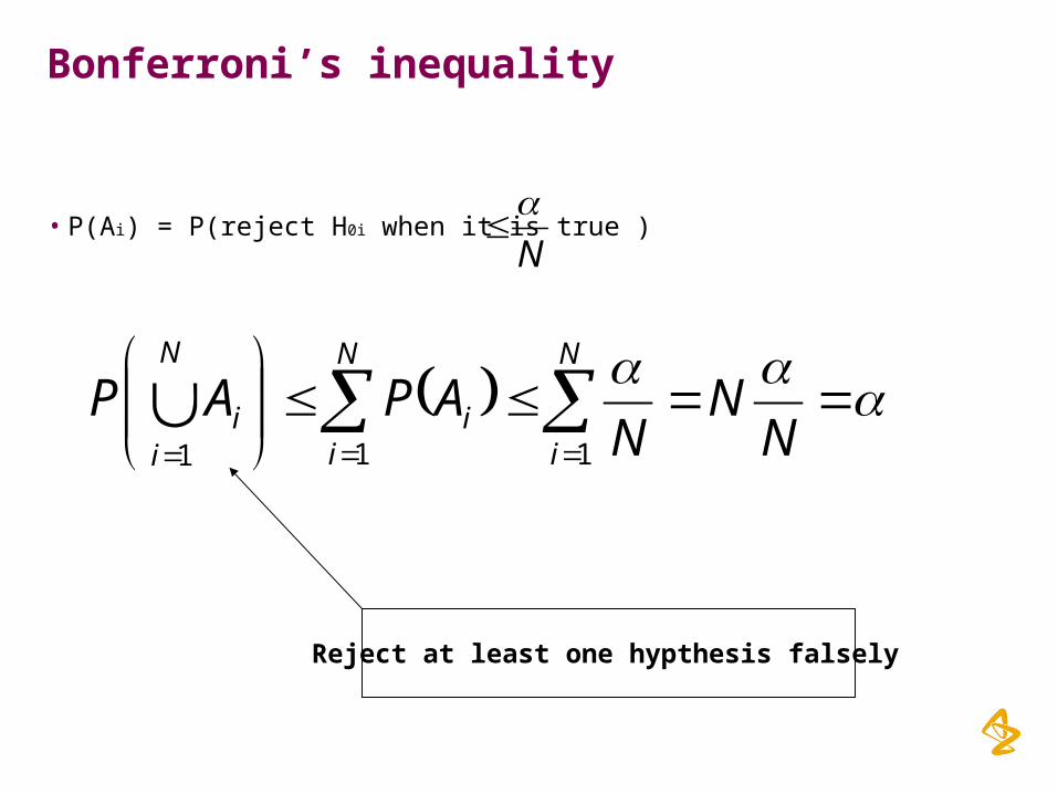
Bonferroni’s inequality
• P(Ai) = P(reject H0i when it is true )
N
NN
APAPN
i
N
ii
N
ii
111
Reject at least one hypthesis falsely
N
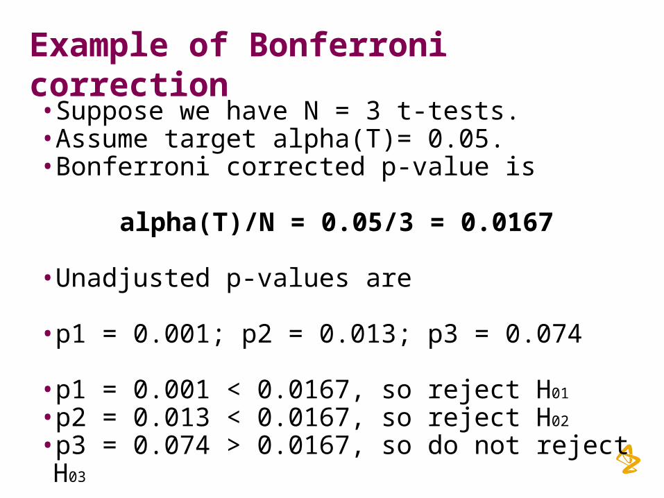
Example of Bonferroni correction
• Suppose we have N = 3 t-tests. • Assume target alpha(T)= 0.05.• Bonferroni corrected p-value is
alpha(T)/N = 0.05/3 = 0.0167
• Unadjusted p-values are
• p1 = 0.001; p2 = 0.013; p3 = 0.074
• p1 = 0.001 < 0.0167, so reject H01
• p2 = 0.013 < 0.0167, so reject H02 • p3 = 0.074 > 0.0167, so do not reject H03
Set area descriptor | Sub level 1
Holm
17 Author | 00 Month Year
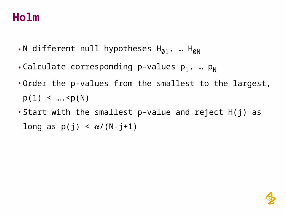
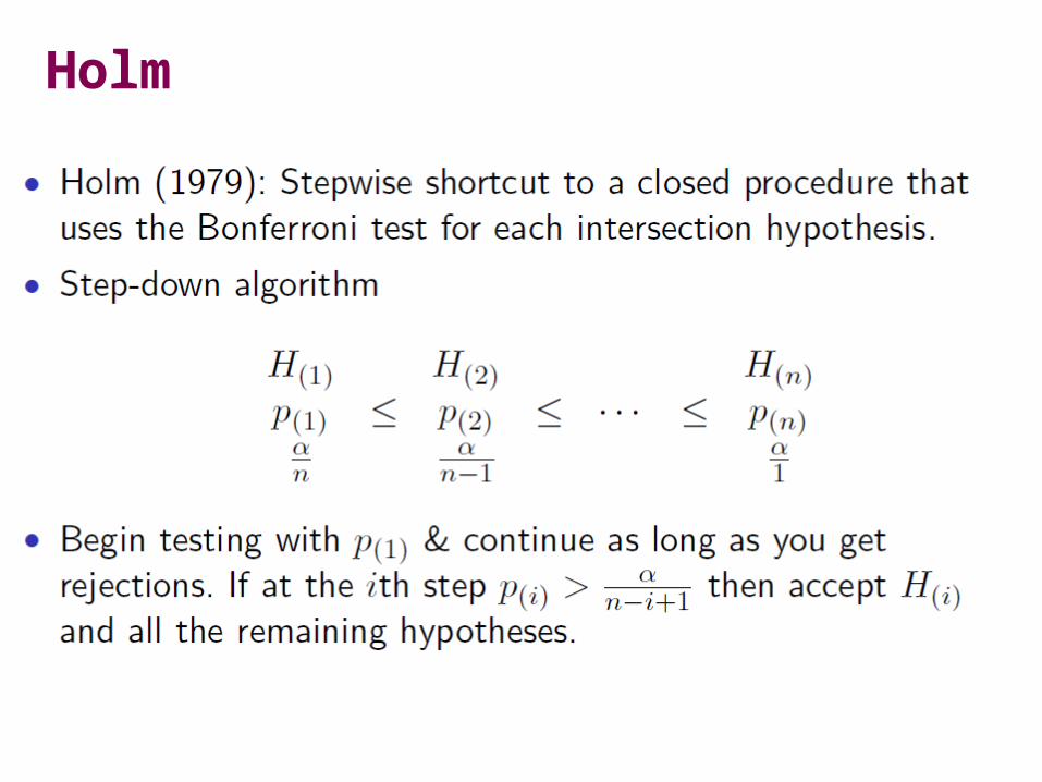
Holm
• N different null hypotheses H01, … H0N
• Calculate corresponding p-values p1, … pN
• Order the p-values from the smallest to the largest, p(1) < ….<p(N)
• Start with the smallest p-value and reject H(j) as long as p(j) < a/(N-j+1)
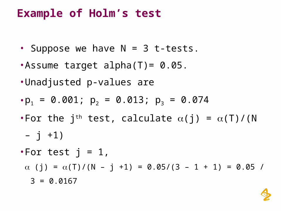
Example of Holm’s test
• Suppose we have N = 3 t-tests.
• Assume target alpha(T)= 0.05.
• Unadjusted p-values are
• p1 = 0.001; p2 = 0.013; p3 = 0.074
• For the jth test, calculate a(j) = a(T)/(N – j +1)
• For test j = 1,
a (j) = a(T)/(N – j +1) = 0.05/(3 – 1 + 1) = 0.05 / 3 = 0.0167
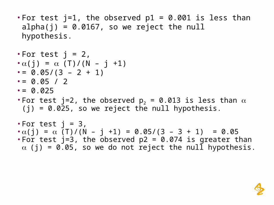
• For test j=1, the observed p1 = 0.001 is less than alpha(j) = 0.0167, so we reject the null hypothesis.
• For test j = 2, • a(j) = a (T)/(N – j +1)• = 0.05/(3 – 2 + 1) • = 0.05 / 2• = 0.025
• For test j=2, the observed p2 = 0.013 is less than a (j) = 0.025, so we reject the null hypothesis.
• For test j = 3, • a(j) = a (T)/(N – j +1) = 0.05/(3 – 3 + 1) = 0.05 • For test j=3, the observed p2 = 0.074 is greater than a (j) = 0.05, so
we do not reject the null hypothesis.
Set area descriptor | Sub level 1
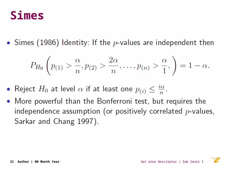
Simes
21 Author | 00 Month Year
Set area descriptor | Sub level 1
Hochberg
22 Author | 00 Month Year
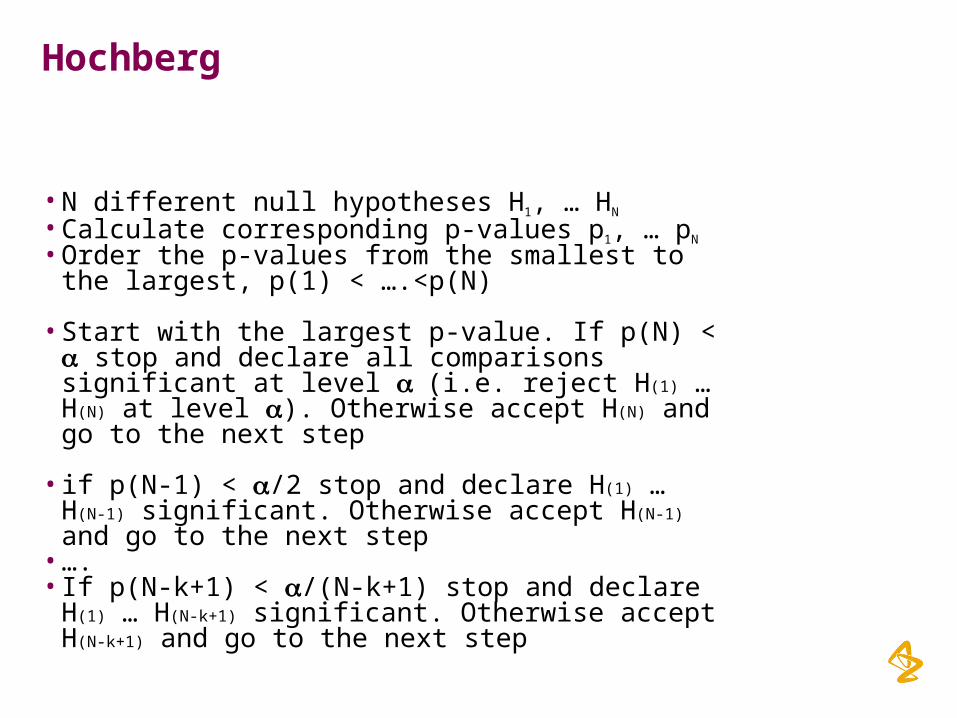
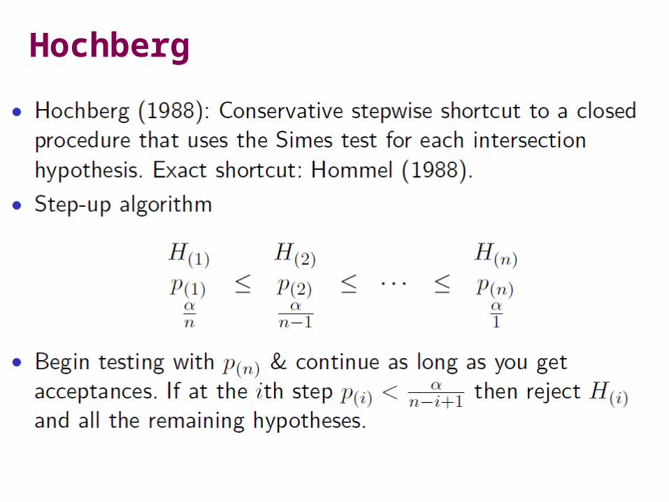
Hochberg
• N different null hypotheses H1, … HN
• Calculate corresponding p-values p1, … pN
• Order the p-values from the smallest to the largest, p(1) < ….<p(N)
• Start with the largest p-value. If p(N) < a stop and declare all comparisons significant at level a (i.e. reject H(1) … H(N) at level a). Otherwise accept H(N) and go to the next step
• if p(N-1) < a/2 stop and declare H(1) … H(N-1) significant. Otherwise accept H(N-1) and go to the next step
• ….• If p(N-k+1) < a/(N-k+1) stop and declare H(1) … H(N-k+1)
significant. Otherwise accept H(N-k+1) and go to the next step
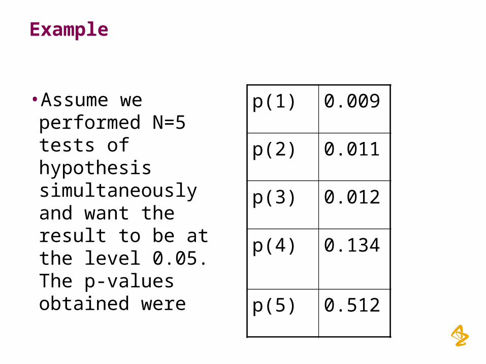
Example
• Assume we performed N=5 tests of hypothesis simultaneously and want the result to be at the level 0.05. The p-values obtained were
p(1) 0.009
p(2) 0.011
p(3) 0.012
p(4) 0.134
p(5) 0.512
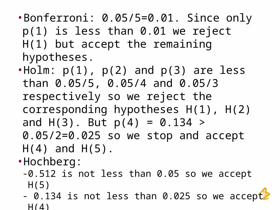
• Bonferroni: 0.05/5=0.01. Since only p(1) is less than 0.01 we reject H(1) but accept the remaining hypotheses.
• Holm: p(1), p(2) and p(3) are less than 0.05/5, 0.05/4 and 0.05/3 respectively so we reject the corresponding hypotheses H(1), H(2) and H(3). But p(4) = 0.134 > 0.05/2=0.025 so we stop and accept H(4) and H(5).
• Hochberg: - 0.512 is not less than 0.05 so we accept H(5)- 0.134 is not less than 0.025 so we accept H(4)- 0.012 is less than 0.0153 so we reject H(1),H(2) and
H(3)
Set area descriptor | Sub level 1
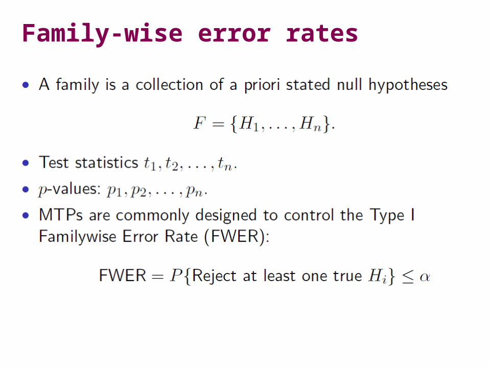
Family-wise error rates
26 Author | 00 Month Year
Set area descriptor | Sub level 1
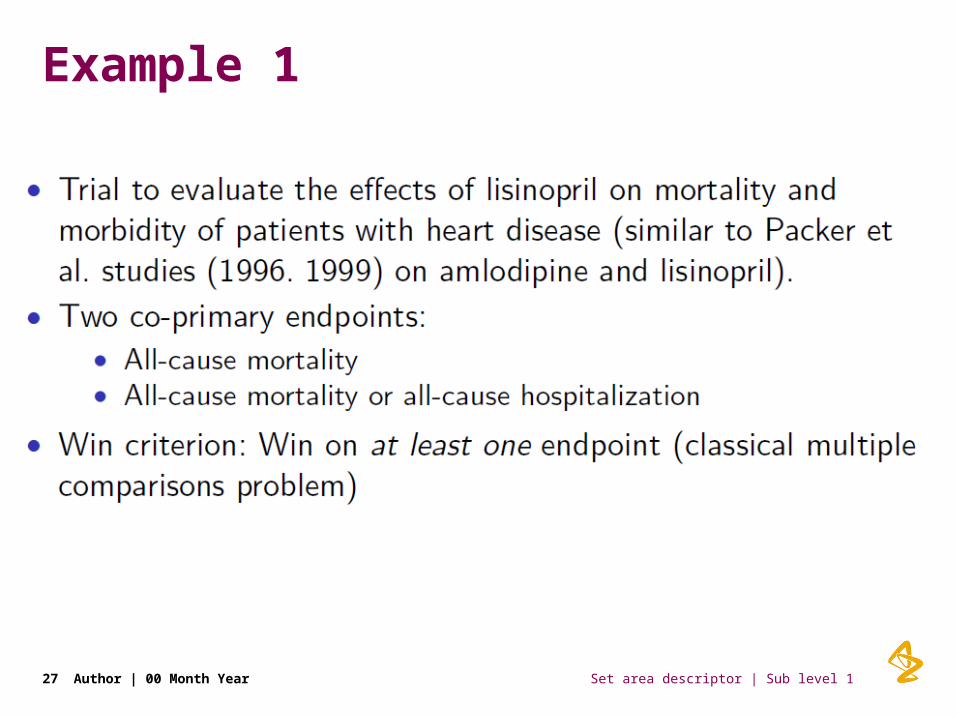
Example 1
27 Author | 00 Month Year
Set area descriptor | Sub level 1
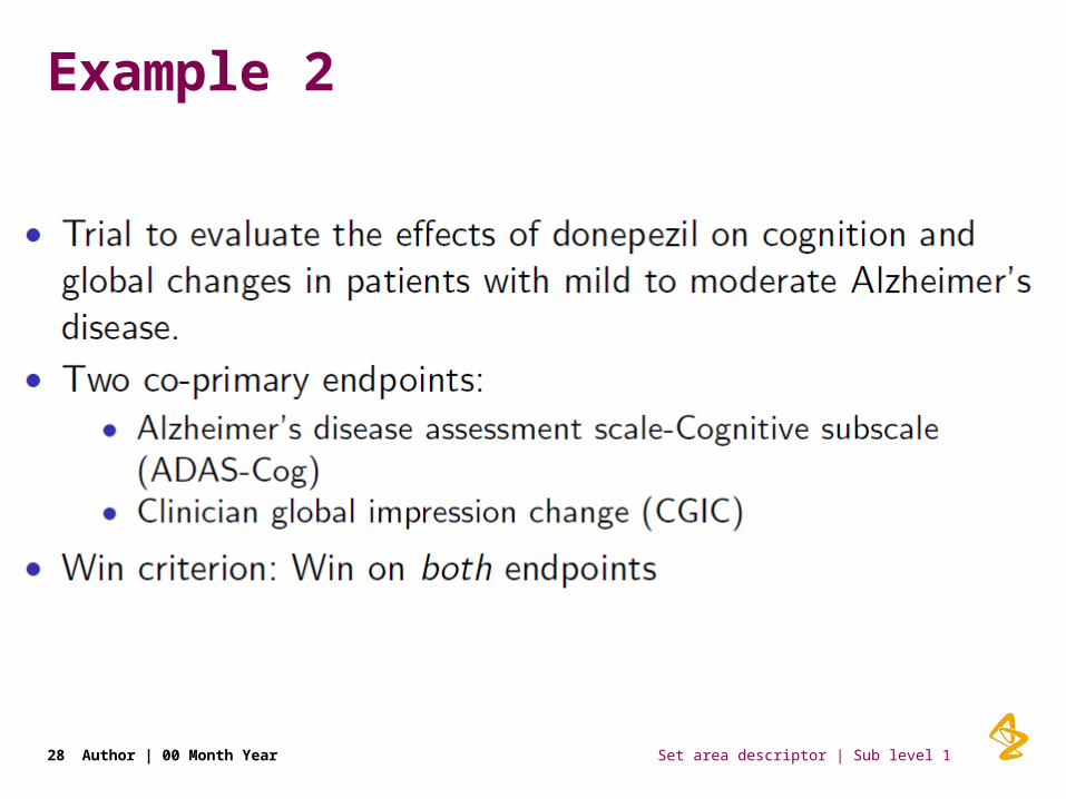
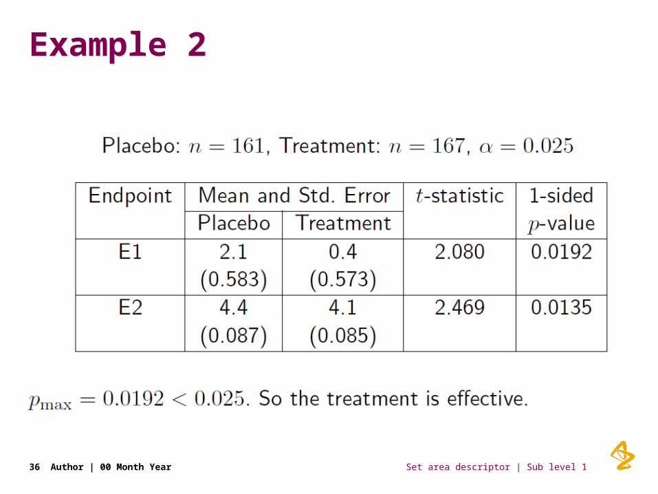
Example 2
28 Author | 00 Month Year
Set area descriptor | Sub level 1
Methods for constructing multiple testing procedures
29 Author | 00 Month Year
Set area descriptor | Sub level 130 Author | 00 Month Year
Set area descriptor | Sub level 1
Fixed sequence
31 Author | 00 Month Year
Set area descriptor | Sub level 1
Fallback
32 Author | 00 Month Year
Set area descriptor | Sub level 1
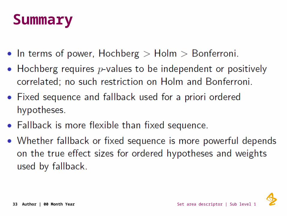
Summary
33 Author | 00 Month Year
Set area descriptor | Sub level 1
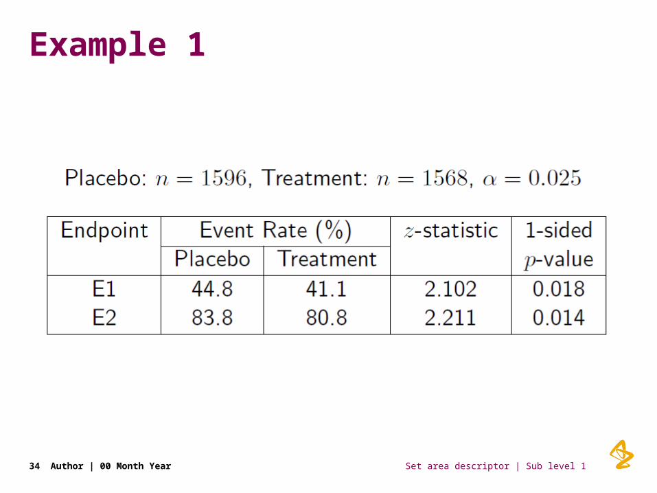
Example 1
34 Author | 00 Month Year

Set area descriptor | Sub level 135 Author | 00 Month Year
Set area descriptor | Sub level 1
Example 2
36 Author | 00 Month Year
Example. Two tests.
•In a heart failure study, two tests were to be performed in a confirmatory analysis. One for testing a treatment effect on death and one to test symptomatic relief using a questionnaire (Quest).
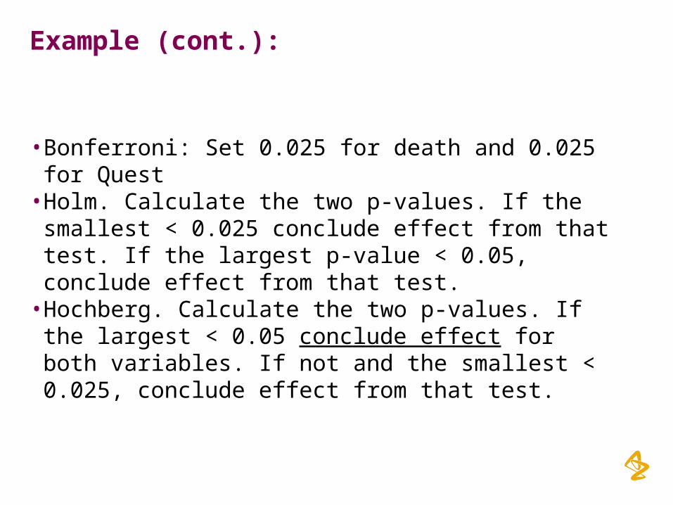
Example (cont.):
• Bonferroni: Set 0.025 for death and 0.025 for Quest• Holm. Calculate the two p-values. If the smallest < 0.025
conclude effect from that test. If the largest p-value < 0.05, conclude effect from that test.
• Hochberg. Calculate the two p-values. If the largest < 0.05 conclude effect for both variables. If not and the smallest < 0.025, conclude effect from that test.

Example (cont.):
• Closed test procedure. Choose one of the variables to test first (must be pre-specified). Calculate the two p-values. If the p-value for the first variable is < 0.05, conclude significance and test the second variable. If this p-value is also < 0.05, then conclude significance also for this variable. If the first p-value > 0.05 then none of the variables are significant.
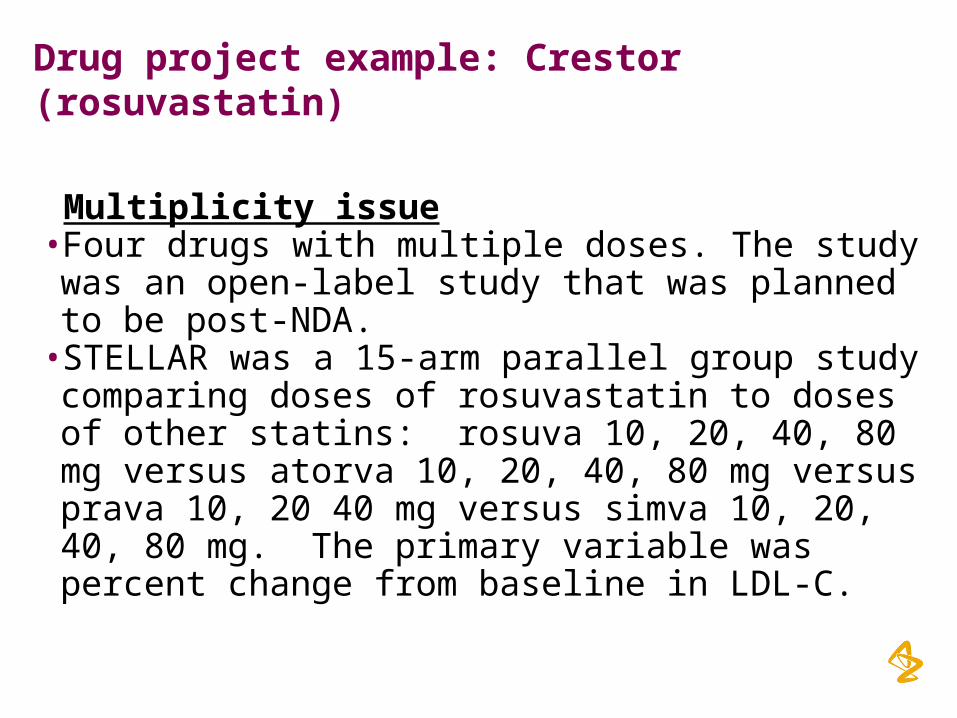
Drug project example: Crestor (rosuvastatin)
Multiplicity issue• Four drugs with multiple doses. The study was an open-label study that was planned to be post-NDA.
• STELLAR was a 15-arm parallel group study comparing doses of rosuvastatin to doses of other statins: rosuva 10, 20, 40, 80 mg versus atorva 10, 20, 40, 80 mg versus prava 10, 20 40 mg versus simva 10, 20, 40, 80 mg. The primary variable was percent change from baseline in LDL-C.
• A commercial request was to compare rosuvastatin to other statins dose-to-dose.
• To address this objective, 25 pairwise comparisons of interest were specified.
• A Bonferroni correction was used to account for multiple comparisons.
• The sample size was estimated considering the Bonferroni correction. It was a large study, with about n=150 per arm.
• Choice of the conservative Bonferroni correction was influenced by the fact that a competitor received a warning letter from the FDA for dose-to-dose promotion from a study that was not designed to do dose-to-dose comparisons.
• There was no discussion with the FDA about correction for multiplicity in STELLAR. Results are considered robust, and they appear in the Crestor label.
References1. Jones PH et al. Comparison of the efficacy
and safety of rosuvastatin versus atorvastatin, simvastatin, and pravastatin across doses (STELLAR trial). Am J Cardiol 2003;92:152-160.
2. McKenney JM et al. Comparison of the efficacy of rosuvastatin versus atorvastatin, simvastatin, and pravastatin in achieving lipid goals: results from the STELLAR trial. Current Medical Research and Opinion 2003;19(8):689-698.


