DESIGN AND ANALYSIS OF IMPELLER BLADE FOR …ijerms.com/DOC/Isues pdf/Archive-2015/May-2015/1_DESIGN...

[Manjunath, 2(5), May 2015] ISSN: 2394-7659 Impact Factor: 2.187 (PIF)

International Journal of Engineering Researches and Management Studies

©International Journal of Engineering Researches and Management Studies http://www.ijerms.com

[1]

DESIGN AND ANALYSIS OF IMPELLER BLADE FOR AXIAL FLOW PUMPS Manjunatha*, Nataraj J R Department of Mechanical Engineering, RVCE, Bengaluru.

ABSTRACT Flows in hydro pumps are three-dimensional, complex and unsteady. Several flow phenomena dominate the

performance, efficiency, noise and vibrations of these machines, and as a result must be accurately predicted. Flow

analyzer are used to give a deeper insight into the underlying physics and enables one to identify and understand the

predominant dynamic mechanisms, both steady and unsteady, which must be controlled and manipulated to enhance

the performance design. In an analysis, an accurate description of both the local spatial and temporal organization of

the flow is essential. Computational Fluid Dynamics (CFD) in industry has come to play a crucial role in predicting

and analyzing fluid flows. This development has been driven by the availability of robust in-house and commercial

CFD codes and by the massive increase in affordable computer speed and memory. This leads to a steady reduction

in the costs of simulations compared to prototyping and model experiments.

A design of axial pump is carried out and analyzed to get the best performance point. The design and performance

analysis of axial pump are chosen because it is the most useful mechanical rotodynamic machine in fluid works

which widely used in domestic, irrigation, industry, large plants and river water pumping system.

In this paper, the pump the head and flow rate of this pump are 8 m and 1000 m3/hour and the speed is 1400 rpm.

The performance analysis of axial pump is carried out after designing the dimensions of axial pump. So, impeller

friction losses, disk friction losses and recirculation losses of centrifugal pump are also considered in performance

analysis of axial pump. The Predicted Head and efficiency is compared with analytical results and it shows the good

agreement.

KEYWORDS: Hydro Pump, CFD, Head And Flow Rate, Losses.

INTRODUCTION Pumps are used in a wide range of industrial and residential applications. Pumping equipment is extremely diverse,

varying in type, size, and materials of construction. There have been significant new developments in the area of

pumping equipment. They are used to transfer liquids from low-pressure to high pressure in this system, the liquid

would move in the opposite direction because of the pressure difference.

OVERVIEW Flows in hydro pumps are three-dimensional, complex and unsteady. Several flow phenomena dominate the

performance, efficiency, noise and vibrations of these machines, and as a result must be accurately predicted. Flow

analyzers are used to give a deeper insight into the underlying physics and enable one to identify and understand the

predominant dynamic mechanisms, both steady and unsteady, which must be controlled and manipulated to enhance

the performance design. In an analysis, an accurate description of both the local spatial and temporal organization of

the flow is essential. Numerical simulation techniques for studying flow phenomena have been evolved from the so-called one-

dimensional (main line or critical path line) calculations and the basic two- and three-dimensional methods (Quasi

3D flow calculations) to the advanced (viscous) 3D Computational Fluid Dynamics. In CFD, the continuity and

Navier-Stokes equations, which describe the motion of a fluid flow, are solved numerically. When predicting flow

fields, CFD simulations provide a fast and cheap way of gaining insight on the distribution of local variables, such

as pressure and velocity, at different operating conditions. Knowledge about local variables, which depend on the

geometrical layout and the initial configuration, allows for predicting integral variables such as pressure rise and

efficiency. This information is of great importance for engineers in design situations with the goal to produce a safe,

reliable, efficient and economically competitive system that meets design point pressure ratio and flows with

adequate stall margin and good efficiency potential.

http://www.ijerms.com/




[2]

Computational Fluid Dynamics (CFD) in industry has come to play a crucial role in predicting and analyzing fluid

flows. This development has been driven by the availability of robust in-house and commercial CFD codes and by

the massive increase in affordable computer speed and memory. This leads to a steady reduction in the costs of

simulations compared to prototyping and model experiments.

The challenge of CFD is thus to accurately predict the flow yield so that the testing of a new design can be done

numerically and hence to minimize experimental testing. This reduces development time and costs considerably.

The fundamental problem of CFD is that the accuracy of the solution depends on the assumptions made when

modeling physical phenomena such as turbulence and unsteady phenomena. For modeling turbulence, most CFD

codes are based on the RANS family (Reynolds Averaged Navier-Stokes). Through a time averaging of the Navier-

Stokes equations, a statistical description of the evolution of the mean quantities is given and a model is applied in

order to take into account the effect of the temporal variations due to turbulence. A wide range of such turbulence

models is available, ranging from simple algebraic models (e.g. Baldwin-Lomax) to two equations models (k-ε and

k-ω models) and more expensive algebraic or full Reynolds stress models. Due to the statistical approach the

standard turbulence models also lack the ability to describe accurately the temporal variation of the flow, especially

if the times scales of the unsteadiness is not much larger than that of the turbulence-scales. These are all phenomena

characterizing flows in turbomachinery. Despite the inadequacy of current turbulence models, designers are

becoming increasingly dependent on (un)steady viscous three-dimensional CFD methods for the design of the

machines. In order to extend the range of confidence in these numerical codes, some means of validation by

comparing the numerical results with data from well-controlled experiments have to be performed. These data will

not only improve the accuracy of the numerical simulations, but also the understanding of the complex physics of

flows in hydropumps. These subjects will be handled in this thesis.

CFD OF HYDRO PUMPS Flows in axial flow pumps are three-dimensional, complex and unsteady. These flow phenomena dominate the

performance, efficiency, noise and vibrations of these machines. In the design phase of axial flow pumps, the

performance requirements are often expressed in terms of pressure rise, efficiency and power consumption and must

be accurately predicted. Before the advent of CFD analysis methods for turbulent flows, designers were able to

achieve high efficiency levels using experimental, empirical, and semi-empirical methods. Drawings were

handmade and the design consisted of long series of operations with long loops of experimentation/redesign.

Nowadays, the drawing board has been replaced by 3D CAD, which leads to great improvements in cost, quality and

delay, allowing quick prototyping and numerical plants definition. Quickly generated grids of axial flow pumps are

used with increasingly predictive CFD codes, with three main objectives:

Comparison between different technical solutions or concepts for product optimization. Some experimentation work

for validation is sometimes necessary in this case.

Advanced understanding of some key physical and technological topics in complex systems. As the results are

usually not sufficiently predictive, the computation is then done in parallel with experimental work, which can be

considered as a complementary tool to computation.

The high levels of performance that have always been economically important for practically all turbomachinery

applications.

The numerical simulations techniques for studying these phenomena have found widespread use, the state of the art

with a perspective to hydromachinery, and more general to turbomachinery, has been reviewed at regular intervals,

for example by Japikse (1976), McNally and Sockol (1985), Lakshminarayana (1991), Hirsch (1994), and by

Denton and Dawes (1999). Further discussions of the different mathematical models applicable to the calculation of

the flow in axial flow pumps, spanning the range of dynamic levels of approximations from the full time-dependent

Navier- Stokes equations to linearized potential flow models and singularity methods, can be found in Cumpsty

(1989). A more comprehensive discussion of flow models is given by Hirsch (1988). Denton (1985), in an

introduction to the application of the Euler equations to turbomachinery flows, gives a concise but very clear





[3]

summary of the classical flow models and solution methods (streamlines curvature, stream function and potential

flow), discussing the properties, advantages, drawbacks, and limitations of each (as applied to 2D flow). Even the first important application of CFD methods around fifteen years ago, the efficiency has increased further

by 1% to 2%. Nevertheless, such small steps in efficiency represent quite large reductions in the remaining sources

of loss. It is probable that unsteady 3D CFD methods with more accurate turbulence models suitable for the flow

structures found in the turbomachinery flows will be essential to make these next small steps. The Computational

Fluid Dynamics (CFD) in industry has become to play a crucial role in predicting and analysing fluid flows. This

development has been driven by the availability of robust in-house and commercial

CFD codes and by the massive increase in affordable computer speed and memory leading to a steady reduction in

the costs of simulations compared to prototyping and model experiments. The challenge of CFD is thus to accurately

predict the flow yield so that the testing of a new design can be done numerically and hence minimize experimental

testing. This reduces development time and costs considerably. The inclusion of numerical testing makes the design

process more cost-efficient and is thus an essential competition parameter.

FLOW ANALYSIS OF AXIAL FLOW PUMP In order to introduce the subject of pump analysis, this chapter emphasizes the numerical approach towards the

prediction of the flow field in pumps. To understand the importance of employing advanced numerical methods for

analysing pump flows a thorough discussion of the general characteristics of the flow field is provided Two-

dimensional Analysis

In principle an axial flow pump is a relatively simple machine consisting of a rotating impeller with a set of stator

blades enclosed within a stationary housing (see figure)

Fig.1. 1 Axial flow pump

In an axial flow pump, the impeller pushes the liquid in a direction parallel to the pump shaft and adds momentum to

the fluid flow through the unit by transfer of energy between the fluid and the rotating propeller blades. It results in a total pressure increases. Axial flow pumps are sometimes called propeller pumps, because they operate essentially

the same as the propeller of a ship. Though simple in concept, axial pumps are very complicated due to the complex

geometry. In order to make an analytical approach to predict the pump flows, the flow field in an axial pump can be

approximated as quasi two-dimensional with streamlines following the geometrical layout of the hub, shroud and

impeller blades. The energy exchange over the impeller can be estimated from a so-called one-dimensional approach

analysing the idealized velocity polygons at the entry and exit of the impeller. The simplest approach to the study of

axial flow compressors is to assume that the flow conditions prevailing at the mean radius fully represent the flow at

all other radii. This two-dimensional analysis at the pitch line can provide a reasonable approximation to the actual

flow, if the ratio of blade height to mean radius is small. When this ratio is large, however, as in the first stage of a

compressor, a three-dimensional analysis is required. Some important aspects of three-dimensional flows in axial





[4]

flow pumps are discussed later. Two further assumptions are that radial velocities are zero, and that the flow is

invariant along the circumferential direction (i.e. there are no “blade-to blade” flow variations).

Figure 1.2 shows a single stage axial-flow. The fluid essentially passes almost axially through a row of moving rotor

blades and a row of fixed stator blades. The incompressible flow assumption is used because the pressure rise of the

stage is usually small. The simplified vector diagram analysis assumes that the flow is one dimensional and leaves

each blade row at relative velocity exactly parallel to the exit blade angle. The velocity diagram of the axial

propeller pump comprises a rotor row followed by a stator row, as shown in figure 1.1. Fluid enters the rotor with

absolute velocity v_1 at angle α_1 (Fig. 1.2). All angles are measured from the axial direction. The sign convention

is such that the angles and velocities as drawn in figure 1.2 will be taken as positive throughout this chapter. The

result of vectorially subtracting the blade speed U with the inlet velocity v_1 is the inlet relative velocity w_1 at

angle〖 β〗_1, which ideally should be parallel to the rotor leading edge (the axial direction is the datum for all

angles). Relative to the blades of the rotor, the flow is turned to the directionβ_2at the outlet with a relative

velocityw_1. Clearly, by adding vectorially the blade speed U onto w_2 gives the absolute velocity from the rotor

v_2 at angle〖 α〗_2. The stator blades deflect the flow towards the axis and the exit velocity is v_3 at angle 〖

α〗_3.

Since there is no radial flow, the inlet and exit rotor speeds are equal, and the one dimensional continuity equation

for uniform, steady flow requires that the axial velocity

Component remains constant. The mass flow Q through the duct is described by ρAiviz , where ρ is the density of

water, Ai is the cross-sectional area of fluid flow cross section i and viz is the absolute axial flow velocity through

the cross-section.

ρA_1 v_1z=ρ A_2 v_2z= ρA_3 v_3z=Q=cte 1.1

Fig.1. 2 Velocity diagrams for a compressor stage

From the geometry of the velocity diagram, the normal velocity (or volume flow) can be directly related to the blade

rotational speed u:

u = ω.r =V_1z.(tgα_1+tgβ_1) = V_2z.( tgα_2+tgβ_2) 1.2

Thus the flow rate can be predicted from the rotational speed ω and the blade angles (β_1, β_2).

P = ω. C = ω. d/dt ((r ) ̅×mv ̅) = ρ. Q. (u_2 v_2t-u_1 v_1t) 1.3

or

H_ideal = P/ρgQ = 1/g (u_2 v_2t-u_1 v_1t) = u/g (∆v_t) 1.4

Applying the angular momentum theorem to the axial flow pump, the power P delivered to the fluid is thus:





[5]

Where m is the mass, ω is the angular velocity, C is the torque, r is the radius from the axis of rotation and is the

absolute velocity vector, v_1t is the velocity component mutually perpendicular to both the rotation axis and the

radius vector, H_ideal is the total head and g is the gravity acceleration.

This is the Euler’s turbomachine equation, showing that the torque C, power P and total head H_ideal are functions

only of the rotor velocities u_1,2and the absolute fluid tangential velocities V_(1t,2t)independent of the axial

velocities through the machine.

Meanwhile, since

u = w_1t v_1t and u =w_(2t ) v_2t, Euler’s relation for the pump head becomes

g H_ideal = u.∆(w_t) 1.5

Strictly speaking, equation 1.5 applies only to a single stream tube of radius r, but it is a good approximation for

very short blades if r denotes the average radius.

THREE-DIMENSIONAL ANALYSIS In the previous paragraph, the fluid motion through the blade row of axial flow pumps was assumed to be two-

dimensional in the sense that radial (i.e. spanwise) velocities did not exist. The flow in the meridional plane was

essentially two-dimensional, and that the effects of the velocities (and the gradients in the velocity or pressure)

normal to the meridional surface were negligible. Moreover, it was tacitly assumed that the flow in a real axial flow

pump could be calculated using a series of two-dimensional solutions for each radius. In doing so it is implicitly

assumed that each annulus corresponds to a stream tube such as depicted in figure 1.3 and that the geometric

relations between the inlet location, r_1, and thickness, dr_1, and the discharge thickness, d_n, and location, r_2, are

known a priori.

Fig.1. 3 Geometry of a meridional stream tube in a pump impeller (Brennen)

In practice this is not the case and quasi-three-dimensional methods have been developed in order to determine the

geometrical relation, r_2 (r_1)These methods continue to assume that the stream surfaces are axisymmetric, and,

therefore, neglect the more complicated three-dimensional aspects of the flow (secondary flows) as will be discussed

below (section 1.5.3: Secondary Flow in Axial Flow Pumps). Nevertheless, these methods allow the calculation of

useful axial flow pump performance characteristics, particularly under circumstances in which the complex

secondary flows are of less importance, such as close to the design condition. When the axial flow pump is operating

far from the design condition, the flow within a blade= passage may have stream surfaces that are far from

axisymmetric. This two-dimensional supposition, in the sense that radial (spanwise) velocities did not exists, is also

not an unreasonable assumption for axial flow pumps of high hub tip ratio. However, with hub-tip ratio less than

about 4/5, radial velocities through a blade row may become appreciable, the consequent redistribution of mass flow

with respect to radius) seriously affecting the outlet velocity profile (and flow angle distribution).

CHARACTERISTICS OF THE 3D FLOW FIELD The flow in an axial flow pump is three-dimensional and should be treated as such in order to achieve a solid

knowledge of the flow field and understand the mechanisms causing the performance do diverge from the ideal case.





[6]

An insight into the physics of the flow can be derived through a discussion with special attention to secondary and

partial load phenomena. When looking into the flow pattern in axial pump impel it is essential first to understand the

influence of the forces acting upon the flow.

FORCES ACTIVE ON THE FLOW The Navier-Stokes equation written in the rotating frame of reference is given by:

(∂W ̅)/∂t + W ̅ W ̅ = - 2ω ̅×W ̅- ω ̅ (ω ̅×r ̅) - ∇^2(W ̅) 1.6

Where 2ω ̅×W ̅ is the Coriolis acceleration and ω ̅ (ω ̅×r ̅) is the centripetal acceleration vector, which is exerted on

the particle because of the rotation of the relative system. In contrast to most other applications the Coriolis

acceleration, is of prime important in the field of hydro machinery. In a rotor, ω ̅×W ̅is zero only if ω and W are

parallel. However, if the relative velocities are everywhere parallel with the axis the corresponding rotor will not be

able to change the energy level of the fluid. The existence of Coriolis acceleration is necessary for producing energy

changes in rotors; in fact, large energy changes require large Coriolis accelerations. These accelerations are also

responsible for the fundamentally different flow patterns in rotor and stator.

The inertia forces (centrifugal and Coriolis forces) have a significant influence on the flow field. The most obvious

effect is the setting up of a radial pressure field due to the centrifugal force acting on the rotating fluid. As indicated

implicitly in the name, this is the main source of the pressure rise obtained in centrifugal pumps. The Coriolis force

is perpendicular to the flow acting from suction to pressure side and causes a buildup of pressure at the pressure side

of the impeller blade making a transfer of torque possible.

PREROTATION Perhaps no aspect of hydro machinery flow is more misrepresented and misunderstood than the phenomenon of

“prerotation”. While this belongs within the larger category of secondary flows (dealt in the section), it is

appropriate to address the issue of prerotation separately, not only because of its importance for the hydraulic

performance, but also because of its interaction with cavitation and stall.

It is first essential to distinguish between two separate phenomena, which both lead to a swirling flow entering the

pump. These two phenomena have very different fluid mechanical origins. Here, we shall distinguish them by the

separate terms, “backflow induced swirl” and “inlet prerotation”. Both imply a swirl component of the flow entering

the pump. Improper entrance conditions and inadequate suction approach shapes may cause the flow in the suction

pipe to spiral from some distance ahead of the actual impeller entrance. This phenomenon is called prerotation, and

it is attributed to various operational and design factors. The flow has axial vorticity (if the axis of rotation is parallel

with the axis of the inlet duct) with a magnitude equal to twice the rate of angular rotation of the swirl motion.

Moreover, there are some basic properties of such swirling flows that are important to the understanding of

prerotation. These are derived from the vorticity transport theorem. In the context of the steady flow in an inlet duct,

this theorem tells us that the vorticity will only change with axial location for two reasons: (a) because vorticity is

diffused into the flow by the action of viscosity, or (b) because the flow is accelerated or decelerated as a result of a

change in the cross-sectional area of the flow. The second mechanism results in an increase in the swirl velocity due

to the stretching of the vortex line, and is similar to the increase in rotation experienced by figure skaters when they

draw their arms closer to their body. When the moment of inertia is decreased, conservation of angular momentum

results in an increase in the rotation rate. Thus, for example, a nozzle in the inlet line would increase the magnitude

of any pre-existing swirl. The backflow is caused by the leakage flow between the tip of the blades of an impeller

and the pump casing. The circumstances are depicted in figure 1.4. Below a certain critical flow coefficient, the

pressure difference driving the leakage flow becomes sufficiently large that the tip leakage jet penetrates upstream

of the inlet plane of the impeller, and thus forms an annular region of “backflow” in the inlet duct (Predin, 2003).

After penetrating upstream a certain distance, the fluid of this jet is then entrained back into the main inlet flow. The

upstream penetration distance increases with decreasing flow coefficient, and can reach many diameters upstream of

the inlet plane.





[7]

Fig.1. 4 Lateral view of impeller inlet flow showing tip leakage flow leading to backflow (Brenne)

Obviously the backflow has a high swirl velocity imparted to it by the impeller blades. But what is also remarkable

is that this vorticity is rapidly spread to the core of the main inlet flow, so that almost the entire inlet flow has a

nonzero swirl velocity. The rapidity with which the swirl vorticity is diffused to the core of the incoming flow

remains something of a mystery, for it is much too rapid to be caused by normal viscous diffusion. It seems likely

that the inherent unsteadiness of the backflow (with a strong blade passing frequency component) creates extensive

mixing which effects this rapid diffusion. However it is clear that this “backflow-induced swirl”, or “prerotation”,

will affect the incidence angles and, therefore, the performance of the pump.

SECONDARY FLOW IN AXIAL FLOW PUMPS The flow in the close vicinity of the blade-tip region of ducted propellers and similar axial flow pumps can be quite

complex due to the presence and dynamic interactions of the tip-leakage vortex, the blade trailing edge vortex, the

gap shear flow, the wall (casing) boundary layer, and the wake from the blade boundary layer. This tip region flow

is important as it has the potential to contribute to a substantial loss in total efficiency and pumping head.

Denton (1993) gave an extensive review of the loss generating mechanisms in turbo machinery. The losses in the

propeller pump can be mainly classified as

1. Profile losses due to blade boundary layers and their separations, possibly including shock/boundary layer

interaction in high speed condition, and wake mixing

2. Endwall boundary layer losses, including secondary flow losses and tip clearance losses

3. Mixing losses due to the mixing of various secondary flows, such as the passage secondary flow (passage vortex)

with leakage flow (or tip leakage vortex)

Secondary flows in the propeller pump are defined normally as the difference between the real flow (including

small-scale turbulent fluctuations) and a primary flow. The primary flow can be referred to, for example, as

idealized axisymmetric flow or midspan flow. The secondary flow arises from the presence of endwall boundary

layer and depends mainly on blade to blade and radial pressure gradients, centrifugal force effects, blade tip

clearance, and the relative motion between the blade ends and the annulus walls. Although the secondary flow

structure in a blade passage has a strong dependence on the incidence angle or flow inlet angle, Reynolds number

and blade profile, their qualitative features are quite general. Normally, the secondary flow relates directly to the

generation and evolution of various concentrated vortices, such as passage vortex, leading edge horseshoe vortex,

corner vortex, tip leading vortex, scraping vortex in an unshrouded rotor, blade trailing edge vortex filament and

shed vortex inside wakes. Hence the following reviews are sectioned in the vortex terminology.

Secondary flow pattern have been presented by many authors in the literature, Hawthorne (1955), Vavra (1960),

Lakshminarayana and Horlock (1963), Salvage (1974), Inoue and Kuroumarou (1984), Kang and Hirsch (1993) and

Zierke et al. (1994). In this review, only the models given by Hawthorne (1955), Lakshminarayana and Horlock

(1963) and Inoue and Kuroumarou (1984) are shown in Figs. 1.5, 1.6 and 1.7.





[8]

Fig.1. 5 Secondary low pattern, after Hawthorne (1955)

Hawthorne’s model describes the classical secondary flow vortex system for the first time (see figure 1.5). This

system presents the components of the vortices in the flow direction when a flow with inlet velocity is deflected

through a cascade. The passage vortex represents the distribution of secondary circulation. The vortex sheet at the

trailing edge is composed of the trailing filament vortices and the trailing shed vorticity.

Fig.1. 6 Secondary flow patterns, after Lakshminarayana and Horlock (1963). In the model of Lakshminarayana and Horlock (1963), figure 1.6, tip leakage flow and relative motion influence are

presented with the tip leakage vortex and scraping vortex. The concentration of the trailing vortex filament is

described. Based on the measurement behind a rotor blade row, Inoue and Kuroumarou (1984), figure 1.7, proposed

a three-dimensional structure of the vortices inside and behind a compressor rotor passage. In the following, losses

in boundary layers and all the secondary flow phenomena will be described one by one.

Fig.1. 7 Secondary flow patterns, after Inoue and Kuroumarou (1984)





[9]

LOSSES IN BOUNDARY LAYERS The efficiency of turbo machine bladings and consequently the overall performance of the machine are strongly

dependent on the boundary layer development on the blades and their separations (if there is any), tip clearance

flows and wakes, which are responsible for energy losses existing in blade passage. For these reasons the knowledge

of the boundary layer and its development plays an important role for the better understanding and further

improvement of axial flow pumps. The flow in axial flow pumps is highly unsteady and turbulent because of the

interaction between the rotor and the stator blade rows due to the wakes and the effect of the potential flow yield. In

particular the periodic influence of the passing wakes plays an important role for the unsteady boundary layer

development on the blades. Generally, there are three fundamental modes for the boundary layer transition from the

laminar to the turbulent state:

The first one is denoted as “natural” transition. It is observed for low levels of free stream turbulence. The transition

process starts with a weak instability in the laminar boundary layer, which develops through various stages to a fully

turbulent boundary layer.

The second mode is known as the “bypass” transition. In this case transition is initiated by disturbances in external

flow (e.g. high free stream turbulence, wakes) and bypasses the “natural” transition. This is the predominated route

of transition in axial flow pumps, where the natural transition process is periodically disturbed by the incoming

wakes (“wake-induced transition”).

A third node occurs if the boundary layer separates. It is therefore known as “separated flow” transition and can be

found in compressors and low-pressure turbines.

There are several parameters influencing the boundary layer development on the blades. These are the properties of

the incoming wakes; free stream turbulence, blade loading, Reynolds number, the profile pressure distribution and

others. Depending on these parameter and as a result of the periodic wake influence, unsteady, highly complex

boundary layer behavior can be observed, where a combination of different forms of transition can be found

(“multimode transition”). Numerous investigations of the boundary layer for steady and unsteady incoming flow is

known from literature.

UNSTEADY PHENOMENA While it is true that cavitation introduces a special set of fluid-structure interaction issues, it is also true that there are

many such unsteady flow problems, which can arise even in the absence of cavitation. One reason these issues may

be more critical in a liquid hydropump is that the large density of a liquid implies much larger fluid dynamic forces.

Typically, fluid dynamic forces scale like ρω2 D4 where ρ is the fluid density, and ω and D are the typical frequency

of rotation and the typical length, such as the span or chord of the impeller blades or the diameter of the impeller.

These forces are applied to blades whose typical thickness is denoted by τ. It follows that the typical structural

stresses in the blades are given by ρω2 D4/τ2, and, to minimize structural problems, this quantity will have an upper

bound, which will depend on the material. Clearly this limit will be more stringent when the density of the fluid is

larger. In many pumps and liquid turbines it requires thicker blades (larger τ) than would be advisable from a purely

hydrodynamic point of view.

LITERATURE REVIEW CFD analysis is very useful for predicting pump performance at various mass-flow rates. For designers, prediction

of operating characteristics curve is most important. All theoretical methods for prediction of efficiency merely give

a value; but one is unable to determine the root cause for the poor performance. Due to the development of CFD

code, one can get the efficiency value as well as observe actual.

〖 LIU Houlin 〗^1 The blade number of impeller is an important design parameter of pumps, which affects the

characteristics of pump heavily. At present, the investigation focuses mostly on the performance characteristics of

axis flow pumps, the influence of blade number on inner flow filed and characteristics of centrifugal pump has not

been understood completely. Therefore, the methods of numerical simulation and experimental verification are used

to investigate the effects of blade number on flow field and characteristics of a centrifugal pump. The model pump





[10]

has a design specific speed of 92.7 and an impeller with 5 blades. The blade number is varied to 4, 6, 7 with the

casing and other geometric parameters keep constant. The inner flow fields and characteristics of the centrifugal

pumps with different blade number are simulated and predicted in non cavitations and cavitations conditions by

using commercial code FLUENT. The impellers with different blade number are made by using rapid prototyping, and their characteristics are tested in an open loop. The comparison between prediction values and experimental

results indicates that the prediction results are satisfied. The maximum discrepancy of prediction results for head,

efficiency and required net positive suction head are 4.83%, 3.9% and 0.36 m, respectively. The flow analysis

displays that blade number change has an important effect on the area of low pressure region behind the blade inlet

and jetwake structure in impellers. With the increase of blade number, the head of the model pumps increases too,

the variable regulation of efficiency and cavitations characteristics are complicated, but there are optimum values of

blade number for each one. The research results are helpful for hydraulic design of centrifugal pump.

〖ANATOLIY A.YEVTUSHENKO et al 〗^2 the article describes research of fluid flow inside an axial-flow pump

that includes guide vanes, impeller and discharge diffuser. Three impellers with different hub ratio were researched.

The article presents the performance curves and velocity distributions behind each of the impeller obtained by

computational and experimental ways at six different capacities. The velocity distributions behind the detached

guide vanes of different hub ratio are also presented. The computational results were obtained using the software

tools CFX-BladeGenPlus and CFXTASCflow. The experimental performance curves were obtained using the

standard procedure. The experimental velocity distributions were obtained by probing of the flow. Good

correspondence of results, both for performance curves and velocity distributions, was obtained for most of the

considered cases. As it was demonstrated, the performance curves of the pump depend essentially on the impeller

hub ratio. Velocity distributions behind the impeller depend strongly on the impeller hub ratio and capacity.

Conclusions concerning these dependencies are drawn.

〖S.Jung,W.H.Jung,S.H.Baek,S.Kang 〗^3 This paper describes the shape optimization of impeller blades for a

anti-heeling bidirectional axial flow pump used in ships. In general, a bidirectional axial pump has efficiency much

lower than the classical unidirectional pump because of the symmetry of the blade type. In this paper, by focusing on

a pump impeller, the shape of blades is redesigned to reach a higher efficiency in a bidirectional axial pump.

〖S Kim,Y S Choi et al 〗^4 In this paper, the interaction of the impeller and guide vane in a series-designed axial-

flow pump was examined through the implementation of a commercial CFD code. The impeller series design refers

to the general design procedure of the base impeller shape which must satisfy the various flow rate and head

requirements by changing the impeller setting angle and number of blades of the base impeller. An arc type

meridional shape was used to keep the meridional shape of the hub and shroud with various impeller setting angles.

The blade angle and the thickness distribution of the impeller were designed as an NACA airfoil type. In the design

of the guide vane, it was necessary to consider the outlet flow condition of the impeller with the given setting angle.

The meridional shape of the guide vane were designed taking into consideration the setting angle of the impeller,

and the blade angle distribution of the guide vane was determined with a traditional design method using vane plane

development. In order to achieve the optimum impeller design and guide vane, three-dimensional computational

fluid dynamics and the DOE method were applied. The interaction between the impeller and guide vane with

different combination set of impeller setting angles and number of impeller blades was addressed by analyzing the

flow field of the computational results.

PROPOSED METHODOLOGY

PRELIMNARY DESIGN OF CENTRIFUGAL PUMP Design method of centrifugal pump are largely based on the application of empirical and semi-empirical rules along

with the use of available information in the form of different types of charts and graphs in the existing literature. The

program developed is best suitable for low specific speed centrifugal pump. Same program is also suitable for the

design of high specific speed and multistage centrifugal pump with few modifications. As the design of centrifugal





[11]

pump involve a large number of interdependent variables, several other alternative designs are possible for same

duty. Hence theoretical investigation supported by accurate experimental studies of the flow through the pump. Impeller as it is the element which transfers energy to the fluid stream influences the performance of the pump.

Different authors have suggested different design procedure, Method of calculation.

The problem of calculation of the dimension of an impeller and hence of the whole pump for given total head may

have several solutions but they are not likely to be of equal merit, when considered from the point of view of

efficiency and production cost.

Each design parameter has been calculated using above procedures and an appropriate value adapt for present

carefully analyzing the calculated values.

DESIGN FACTORS OF THE PUMP The factors which affect the performance of the pump are:

1)Hub ratio 2) Number of vanes 3) Vane thickness 4) Setting of vanes to the hub 5) Pump casing

Impeller Hub ratio:- This is the most important design factor controlling specific speed of an impeller. It is the ratio of hub diameter (at

exit) to the outer diameter of the vane (at entrance) i.e. D_2i/D_1 for axial flow pumps above n_s=180

Fig 3.1 : Hub ratio

Number of vanes:- Experimental results obtained by many researchers confirm that with minimum number of vanes the efficiency is

maximum. More of vanes will restrict the free area of flow causing reduction in capacity and decreases in efficiency.

However in practice 2 to 5 vanes are generally provided.

The chord spacing ratio l/t is another factor linked with number of vanes needs proper selection as it varies along the

radius, increasing towards the hub for mechanical reasons.

Fig 3.2: Chord spacing of vanes





[12]

Specific speed:- Pump specific speed is the speed of an impeller in revolutions per minute at which a geometrically similar impeller

would run if it were of such a size as to discharge one gallon per minute against one foot head square.

Ns = (N√Q)/H^(3/4)

Where

Ns : specific speed in rpm

Q: Flow rate in m^3/hour

H: Head in m

DESIGN PROCEDURE FOR AN AXIAL FLOW IMPELLER Knowledge of the theory of impeller vane action and the relationship among several design elements is essential in

the selection of the design constants necessary to achieve the desired performance with best possible efficiency. The

design procedure involves the following steps

To meet a given set of head capacity requirements, the speed (r.p.m) is selected. Thus the specific speed of the

impeller is fixed. Due consideration should be given to the head range the proposed pump should cover in future

application under the most adverse suction consideration.

The speed constants and capacity constants are chosen next. These constants having been established, the meridional

velocity and impeller diameter calculated and the impeller profile can be drawn.

The impeller vane profile, both vane curvature and vane twist, are drawn after the entrance and discharge vane

angles for several streamlines are established from Euler’s entrance and exit velocity triangles.

The design pump is one horse power motor drive single-stage centrifugal pump. Impeller is designed on the basic of

design flow rate, pump head and pump specific speed. So, the design data are required to design the centrifugal

pump. For design calculation, the design parameters are taken as follows:

Flow rate, Q = 1000 m3/hour

Head, H = 8 m

Pump speed, n = 1400 rpm

Gravitational acceleration, g = 9.81 m/s2

Density of water, ρ= 1000 kg/m3

DESIGN OF IMPELLER

1. Specific speed:- Specific speed of the pump is computed based on the power as well as discharge; different authors expressed the

design parameter as function of specific speed

N_s= (N√Q)/H ^ (3/4) 2.1

N_s=155.117 rpm

Where N = speed at pump shaft rotated.

Q = discharge in m3 / sec

H = net head in m.

For given data N= 155.117 RPM

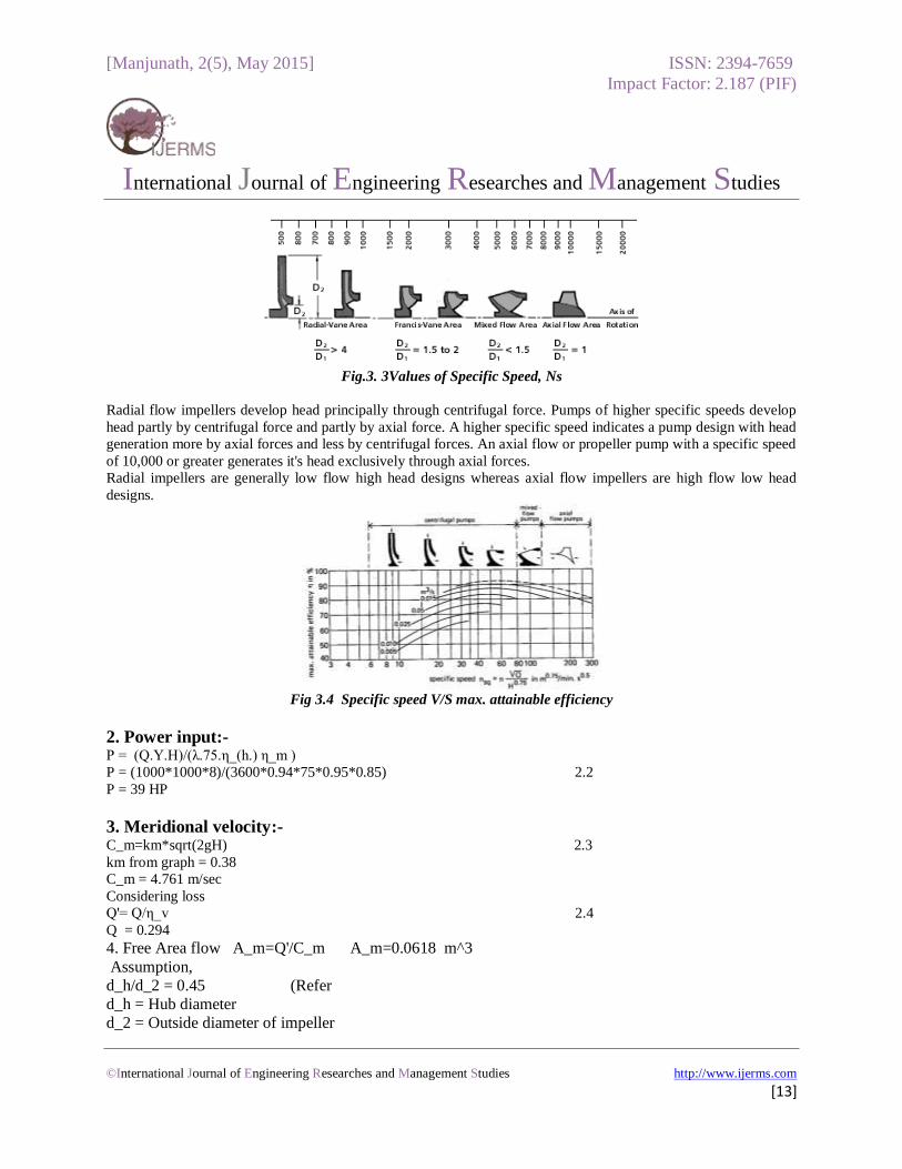
The specific speed determines the general shape or class of the impeller as depicted in Fig. 3. As the specific speed

increases, the ratio of the impeller outlet diameter, D2, to the inlet or eye diameter, Di, decreases. This ratio becomes

1.0 for a true axial flow impeller.





[13]

Fig.3. 3Values of Specific Speed, Ns

Radial flow impellers develop head principally through centrifugal force. Pumps of higher specific speeds develop

head partly by centrifugal force and partly by axial force. A higher specific speed indicates a pump design with head

generation more by axial forces and less by centrifugal forces. An axial flow or propeller pump with a specific speed

of 10,000 or greater generates it's head exclusively through axial forces.

Radial impellers are generally low flow high head designs whereas axial flow impellers are high flow low head

designs.

Fig 3.4 Specific speed V/S max. attainable efficiency

2. Power input:- P = (Q.Y.H)/(λ.75.η_(h.) η_m )

P = (1000*1000*8)/(3600*0.94*75*0.95*0.85) 2.2

P = 39 HP

3. Meridional velocity:- C_m=km*sqrt(2gH) 2.3 km from graph = 0.38

C_m = 4.761 m/sec

Considering loss

Q'= Q/η_v 2.4

Q = 0.294

4. Free Area flow A_m=Q'/C_m A_m=0.0618 m^3

Assumption,

d_h/d_2 = 0.45 (Refer

d_h = Hub diameter

d_2 = Outside diameter of impeller





[14]

d_h = 0.314 m

d_2 = 0.141m

Axial pump -no inlet guide vane producing pre-whirl α_1=90 C_u1=0

5. Effective impeller diameter:- D_m=〖〖√D〗_2〗^"2" +〖 D_h〗^2/2 2.5

D_m= 0.54 m

6. Streamlines:- Average velocity = Q/Area 2.6

= 3.66 m/sec

7. Blade angle:- Inlet angle: Fluid at inlet assumed no pressure whirl

Tanβ_1= C_m/u_1 2.7

(a)Tanβ_(1_A1A2 )= C_m/u_1A = 4.7/10.26 (b) Tanβ_(1_B1B2 )= C_m/u_1B

β_(1_A1A2 )= 24.6 ̊ β_(1_B1B2 )= 18.2 ̊

(c)Tanβ_(1_C1C2 ) = C_m/u_1C (d) Tanβ_(1_D1D2 )= C_m/u_1D

〖 β〗_(1_C1C2 )= 14.95⁰ β_(1_D1D2 ) = 12.98⁰ (e)Tanβ_(1_E1E2 ) = C_m/u_1E

β_(1_E1E2 ) =11.68⁰

Figure 3.5 Inlet Velocity Triangles

8. Relative velocity:-

W_1 = C_m1/〖Sinβ〗_1 2.8

(a)W_1A = C_m1/〖Sinβ〗_1A = 4.7/Sin〖(〖24.6〗^0)〗 = 11.30

(b)〖 W〗_1B= C_m1/〖Sinβ〗_1B = 4.7/(Sin (〖18.2〗^0)) = 15.17

(c)W_1C = C_m1/〖Sinβ〗_1c = 4.7/Sin〖(〖14.95〗^0)〗 = 18.21

(d)W_1D = C_m1/〖Sinβ〗_1D = 4.7/Sin〖(〖12.98〗^0)〗 = 20.92

(e)W_1E = C_m1/〖Sinβ〗_1E = 4.7/Sin〖(〖11.68〗^0)〗 = 23.21

9. Outlet angle:- we assume C_m1 = C_m2

C_u3= (gH_th)/u_2 2.9





[15]

The value of β_3 is calculated from the formula tanβ_3 = C_m2/(u_2-C_u3 )

2.10

tanβ_3A = C_m2/(u_2-C_u3 ) = 4.7/(22.72-4.14) = 14.19⁰ In order to establish the constructional angle we require the ratio

C_u2/C_u3 = 1+ C_p = H_th∞/H_th 2.11

C_u2= C_u3 (1+C_p)

〖 C〗_p= Ψ' r/ze where e – axial length of blade 2.12

e = (d_2-d_h)/4 = 170/4 = 42.5 2.13

Ψ' = 2 assumed

C_u2= C_u3 (1+C_p) 2.14

C_p= Ψ' r/ze = (2×112.5)/(3×42.5) = 1.76

Therefore C_u2= C_u3 (1+C_p) 2.15

(a)C_(〖u2〗_A1A2 )= 9.18(1+1.76) (b) C_(〖u2〗_B1B2 )= 6.55(1+1.76)

C_(〖u2〗_A1A2 ) =25.33 C_(〖u2〗_B1B2 ) =18.078

(c) C_(〖u2〗_C1C2 )= 5.35(1+1.76) (d) C_(〖u2〗_D1D2 )= 4.62(1+1.76)

C_(〖u2〗_C1C2 )=14.76 C_(〖u2〗_D1D2 )= 12.75

(e) C_(〖u2〗_E1E2 )= 4.14(1+1.76)

C_(〖u2〗_E1E2 ) =11.42

Outlet angle:- tanβ_2=C_m2/(u_2-C_u2 ) = 4.7/(17.60-14.76) =58.85⁰ 2.16

〖 W〗_2= Cm2/sinβ2 = 4.7/sin〖58.85⁰〗 = 5.49 2.17

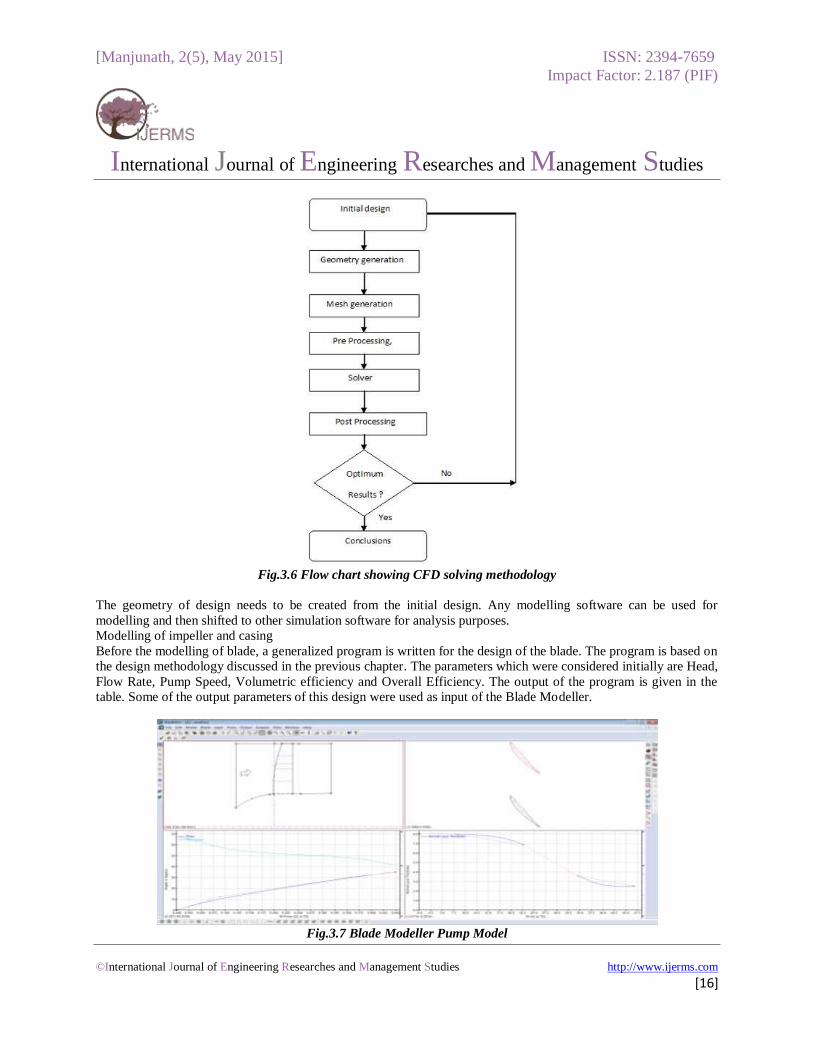
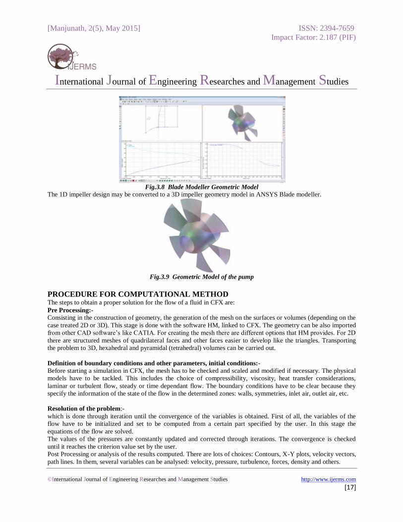
GEOMETRIC MODELLING OF PUMP In order to obtain better design in CFD, following procedure is applied so that fluid flow can easily be modelled.

Initial design of the model is a planning decision and the geometry is generated depending on these initial design

considerations, using either CFD modelling tools or other Design tools. The first task to accomplish in a numerical

flow simulation is the definition of the geometry, followed by the grid generation. This step is the most important step for the study of an isolated impeller assuming an axis symmetric flow simplifies the domain to a single blade

passage.





[16]

Fig.3.6 Flow chart showing CFD solving methodology

The geometry of design needs to be created from the initial design. Any modelling software can be used for

modelling and then shifted to other simulation software for analysis purposes.

Modelling of impeller and casing

Before the modelling of blade, a generalized program is written for the design of the blade. The program is based on

the design methodology discussed in the previous chapter. The parameters which were considered initially are Head,

Flow Rate, Pump Speed, Volumetric efficiency and Overall Efficiency. The output of the program is given in the

table. Some of the output parameters of this design were used as input of the Blade Modeller.

Fig.3.7 Blade Modeller Pump Model





[17]

Fig.3.8 Blade Modeller Geometric Model

The 1D impeller design may be converted to a 3D impeller geometry model in ANSYS Blade modeller.

Fig.3.9 Geometric Model of the pump

PROCEDURE FOR COMPUTATIONAL METHOD The steps to obtain a proper solution for the flow of a fluid in CFX are:

Pre Processing:-

Consisting in the construction of geometry, the generation of the mesh on the surfaces or volumes (depending on the

case treated 2D or 3D). This stage is done with the software HM, linked to CFX. The geometry can be also imported

from other CAD software’s like CATIA. For creating the mesh there are different options that HM provides. For 2D

there are structured meshes of quadrilateral faces and other faces easier to develop like the triangles. Transporting

the problem to 3D, hexahedral and pyramidal (tetrahedral) volumes can be carried out.

Definition of boundary conditions and other parameters, initial conditions:-

Before starting a simulation in CFX, the mesh has to be checked and scaled and modified if necessary. The physical

models have to be tackled. This includes the choice of compressibility, viscosity, heat transfer considerations,

laminar or turbulent flow, steady or time dependant flow. The boundary conditions have to be clear because they

specify the information of the state of the flow in the determined zones: walls, symmetries, inlet air, outlet air, etc.

Resolution of the problem:-

which is done through iteration until the convergence of the variables is obtained. First of all, the variables of the

flow have to be initialized and set to be computed from a certain part specified by the user. In this stage the

equations of the flow are solved.

The values of the pressures are constantly updated and corrected through iterations. The convergence is checked

until it reaches the criterion value set by the user.

Post Processing or analysis of the results computed. There are lots of choices: Contours, X-Y plots, velocity vectors,

path lines. In them, several variables can be analysed: velocity, pressure, turbulence, forces, density and others.





[18]

MESHING GENERATION Mesh generation (Girding) is the process of subdividing a region to be modelled into a setoff small control volumes.

Associated with each control volume there will be one or more values of the dependent flow variables (e.g.,

velocity, pressure, temperature, etc.) Usually these represent some type of locally averaged values. Numerical

algorithms representing approximations to the conservation laws of mass, momentum and energy are then used to

compute these variables in each control volume.

Meshing is a method to define and break up the model into small elements. In general, a finite element model is

defined by a mesh network, which is made up of the geometric arrangement of elements and nodes. Nodes represent

points at which features such as displacements are calculated. Elements are bounded by sets of nodes, and define

localized mass and stiffness properties of the model. Elements are also defined by mesh numbers, which allow

references to be made to corresponding deflections, stresses, pressures, temperatures at specific model locations.

The traditional method of mesh generation is block-structure (multi-block) mesh generation. The block-structure

approach is simple and efficient technique of mesh generation The topology is a structure of blocks that acts as a framework for positioning mesh elements. Topology blocks

represent sections of the mesh that contain a regular pattern of hexahedral (hex) elements. They are laid out adjacent

to each other without overlap or gaps, with shared edges and corners between adjacent blocks, such that the entire

domain is filled. By using topology blocks to control the placement of hex elements, a valid hexmesh can be

generated to fill a domain of arbitrary shape. The topology is invariant from hub to shroud and is viewed/edited on

2-D layers which are located at various spanwise stations. The topology blocks can be arranged in a regular

(structured) pattern, an irregular (unstructured) pattern, or in a pattern consisting of structured patches and

unstructured patches. The choice of which approach should be followed should be based on whichever method

minimizes the maximum skew of the topology blocks, since the skew in the hex elements of the mesh is directly

related. The topology should then be investigated at various layers (especially the hub and shroud layers) to check its

quality since the mesh quality is directly dependent on topology. Topology blocks generally contain the same

number of mesh elements along each side. The mesh elements vary in size across topology blocks in a way that produces a smooth transition within and between blocks. This is accomplished by shifting the nodes toward, or away

from, certain block edges.

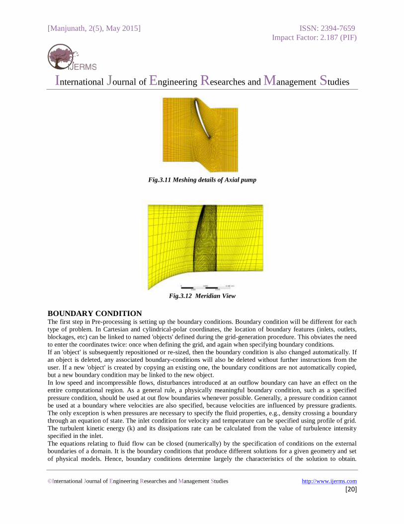
A 3D hexahedral mesh is generated using Hyper Mesh pre-processor.

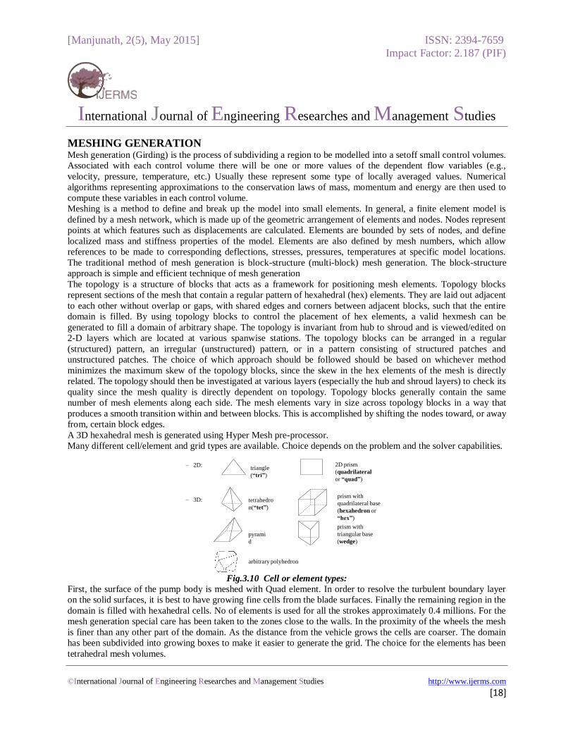
Many different cell/element and grid types are available. Choice depends on the problem and the solver capabilities.

Fig.3.10 Cell or element types:

First, the surface of the pump body is meshed with Quad element. In order to resolve the turbulent boundary layer

on the solid surfaces, it is best to have growing fine cells from the blade surfaces. Finally the remaining region in the

domain is filled with hexahedral cells. No of elements is used for all the strokes approximately 0.4 millions. For the

mesh generation special care has been taken to the zones close to the walls. In the proximity of the wheels the mesh

is finer than any other part of the domain. As the distance from the vehicle grows the cells are coarser. The domain

has been subdivided into growing boxes to make it easier to generate the grid. The choice for the elements has been

tetrahedral mesh volumes.

• Many different cell/element and grid types are available. Choice depends on the problem

and the solver capabilities.

• Cell or element types:

– 2D:

– 3D:

triangle

(“tri”)

2D prism

(quadrilateral

or “quad”)

tetrahedro

n(“tet”)

pyrami

d

prism with

quadrilateral base

(hexahedron or

“hex”)

prism with

triangular base

(wedge)

arbitrary polyhedron





[19]

Representations of the different surface meshes that take part in the study are depicted in the following detailed

figures

CFX-TURBO GRID CFX-TurboGrid enables to generate computational grids quickly through the automatic management of grid

topology, periodic boundaries, and grid attachment.

Grid topology is managed through the selection of a pre-defined template. Templates are available allowing for

optimal meshing of most turbomachines. Suitable templates are provided for low- and high-solidity axial, radial,

[14] and mixed-flow blade geometries. Templates are also provided for multi-bladed (split) flow passages and for

blade tip clearance.

Periodic boundaries are managed ensuring both physical and topological periodicity. Physical periodicity is

maintained through the use of a ``master-slave'' relationship between opposing periodic control points. If a control

point on the periodic boundary is moved, the corresponding control point on the opposite periodic boundary is

moved by the same amount. The number of grid elements along two related curves on the periodic boundaries is

always kept equal. If grid elements are added to a control curve on a periodic boundary, the opposing periodic

control curve receives the same increment in grid element count. Grid attachment between the sub-grids of a multi-block domain and between corresponding periodic boundaries is

automatically performed during mesh creation for all connections

CFX-TurboGrid requires the input of three data files (Profile, Hub, and Shroud) to define the flow path and blade

geometry

The ``Profile'' data file contains the blade ``profile'' or ``rib'' curves in Cartesian or Cylindrical form. The profile

points are listed, line-by-line, in free-format ASCII style in a closed-loop surrounding the blade.

The hub and shroud curve runs upstream to downstream and must extend upstream of the blade leading edge and

downstream of the blade trailing edge

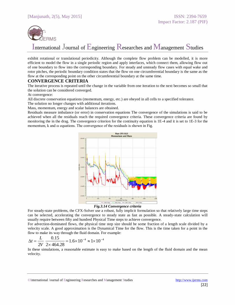
COMPUTATIONAL GRID In RANS simulations, the choice of mesh type is of critical importance. In this study, the widely used structured

body-fitted curvilinear meshes are chosen rather than unstructured tetrahedral meshes. Body-fitted structured meshes

are well suited for viscous flow because they can be easily compressed near all solid surfaces. Using a multiblock

approach, they are also convenient for discretizing the flow passages in turbomachinery flows with rather

straightforward geometries, which includes blade tip clearances and relative motion.

The grid used for the present study is shown in Figure 7.1 with the meridional view and Figure 7.2 with the blade-to-

blade view. The grid for the axial pump consists of 68308 rotors.

In addition, single passage of Rotor consists of 69 mesh points in the stream-wise direction, 44 points in the blade-

to-blade direction, and 26 points in the span-wise direction. A total of 6 points are used in the span-wise direction to

describe the tip-clearance between the rotor blades and the casing.





[20]

Fig.3.11 Meshing details of Axial pump

Fig.3.12 Meridian View

BOUNDARY CONDITION The first step in Pre-processing is setting up the boundary conditions. Boundary condition will be different for each

type of problem. In Cartesian and cylindrical-polar coordinates, the location of boundary features (inlets, outlets,

blockages, etc) can be linked to named 'objects' defined during the grid-generation procedure. This obviates the need

to enter the coordinates twice: once when defining the grid, and again when specifying boundary conditions.

If an 'object' is subsequently repositioned or re-sized, then the boundary condition is also changed automatically. If

an object is deleted, any associated boundary-conditions will also be deleted without further instructions from the

user. If a new 'object' is created by copying an existing one, the boundary conditions are not automatically copied,

but a new boundary condition may be linked to the new object.

In low speed and incompressible flows, disturbances introduced at an outflow boundary can have an effect on the

entire computational region. As a general rule, a physically meaningful boundary condition, such as a specified

pressure condition, should be used at out flow boundaries whenever possible. Generally, a pressure condition cannot

be used at a boundary where velocities are also specified, because velocities are influenced by pressure gradients.

The only exception is when pressures are necessary to specify the fluid properties, e.g., density crossing a boundary

through an equation of state. The inlet condition for velocity and temperature can be specified using profile of grid.

The turbulent kinetic energy (k) and its dissipations rate can be calculated from the value of turbulence intensity

specified in the inlet.

The equations relating to fluid flow can be closed (numerically) by the specification of conditions on the external

boundaries of a domain. It is the boundary conditions that produce different solutions for a given geometry and set

of physical models. Hence, boundary conditions determine largely the characteristics of the solution to obtain.





[21]

Therefore, it is important to set boundary conditions that accurately reflect the real situation to obtain accurate

results. The different types of boundary conditions as shown in Fig

SOLID WALL At a solid wall, the analytic boundary condition that the wall is adiabatic and there is zero normal component of the

relative velocity is used. In addition, the tangent component of the relative velocity is zero for a viscous flow.

Computationally, this is implemented by simply allowing no mass flux through the solid wall faces and setting the

velocity in the cells such that flow tangency is enforced on the solid wall for inviscid cases or zero tangent velocity

for viscous cases.

INLET AND EXIT Five independent variables must be given at each inlet and exit boundary to solve the flow governing equations in

three-dimensions. The number and type of conditions that need to be specified from information extended to the

flow, as well as that which must be calculated from information from the interior flow itself can be determined from

an examination of the characteristic paths bringing information to each boundary cell.

At the inlet boundary, four of the five independent flow variables must be specified for axially subsonic inlet flows.

Similarly, to actual experimental setups, total pressure and total temperature are fixed. The other flow variable must

be extrapolated from the interior flow field according to a characteristic analysis.

Fig 3.13 Boundary conditions

On the other hand, only the pressure is specified at the exit boundary for subsonic flows. The other variables on the

cells adjacent to the exit boundary are determined by simple extrapolation of density and three components of

velocity from the interior cells adjacent to the boundary for the Navier-Stokes equations. For supersonic outlet

flows, all variables are extrapolated from the interior flow.

PERIODIC BOUNDARY In many practical situations, a portion of the flow field is repeated in many identical regions. The flow around a

single turbine blade in a rotating machine, or heat exchanger fin is such examples. These problems are said to





[22]

exhibit rotational or translational periodicity. Although the complete flow problem can be modelled, it is more

efficient to model the flow in a single periodic region and apply interfaces, which connect them, allowing flow out

of one boundary to flow into the corresponding boundary. For steady and unsteady flow cases with equal wake and

rotor pitches, the periodic boundary condition states that the flow on one circumferential boundary is the same as the

flow at the corresponding point on the other circumferential boundary at the same time.

CONVERGENCE CRITERIA The iterative process is repeated until the change in the variable from one iteration to the next becomes so small that

the solution can be considered converged.

At convergence:

All discrete conservation equations (momentum, energy, etc.) are obeyed in all cells to a specified tolerance.

The solution no longer changes with additional iterations.

Mass, momentum, energy and scalar balances are obtained.

Residuals measure imbalance (or error) in conservation equations The convergence of the simulations is said to be

achieved when all the residuals reach the required convergence criteria. These convergence criteria are found by

monitoring the in the drag. The convergence criterion for the continuity equation is 1E-4 and it is set to 1E-3 for the

momentum, k and ω equations. The convergence of the residuals is shown in Fig.

Fig.3.14 Convergence criteria

For steady-state problems, the CFX-Solver use a robust, fully implicit formulation so that relatively large time steps

can be selected, accelerating the convergence to steady state as fast as possible. A steady-state calculation will

usually require between fifty and hundred Physical Time steps to achieve convergence.

For advection-dominated flows, the physical time step size should be some fraction of a length scale divided by a

velocity scale. A good approximation is the Dynamical Time for the flow. This is the time taken for a point in the

flow to make its way through the fluid domain. For example:

V

Lt

2 44 101106.1

28.4642

15.0

In these simulations, a reasonable estimate is easy to make based on the length of the fluid domain and the mean

velocity.





[23]

RESULTS AND DISCUSSIONS

Flow distribution in impeller at different span

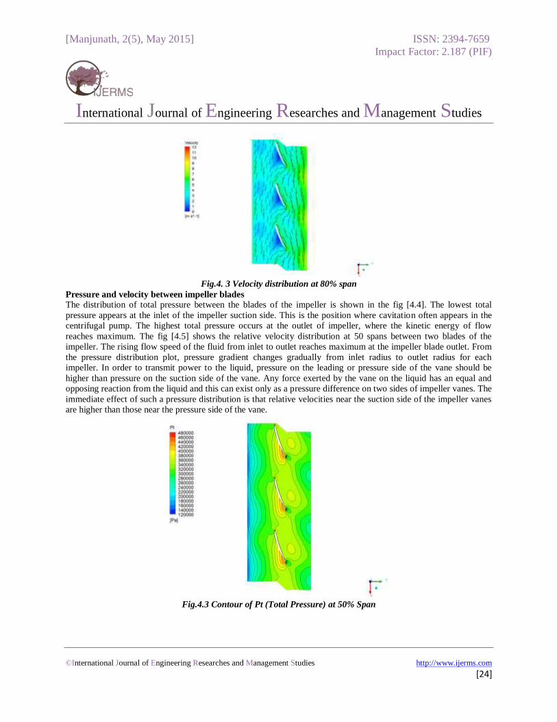
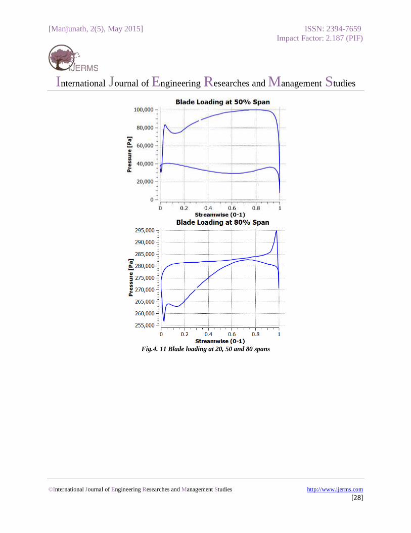
The pressure increases gradually along stream wise direction within rotor passage and has higher pressure in

pressure side than suction side of the impeller blade. However, the pressure developed inside the impeller is not so uniform. The isobar lines are not all perpendicular to the pressure side of the blade inside the impeller passage; this

indicated that there could be a flow separation because of the pressure gradient effect. The fig [4.1 and 4.2] shows

the pressure distribution within the impeller at 50 %.

Fig.4. 1 Pressure distribution at 50 % span

Velocity also increases gradually along stream wise direction within the impeller passage. As the flow enters the

impeller eye, it is diverted to the blade-to-blade passage. The flow at the entrance is not shockless because of the

unsteady flow entering the impeller passage. The separation of flow can be seen at the blade leading edge. Since, the

flow at the inlet of impeller is not tangential to the blade, the flow along the blade is not uniform and hence the

separation of flow takes place along the surface of blade. Here it can be seen that flow separation is taking place on

both side of the blade, ie, pressure and suction side as shown in fig [4.2 and 4.3].

Fig.4. 2 Velocity distribution at 20, 50 % span





[24]

Fig.4. 3 Velocity distribution at 80% span

Pressure and velocity between impeller blades

The distribution of total pressure between the blades of the impeller is shown in the fig [4.4]. The lowest total

pressure appears at the inlet of the impeller suction side. This is the position where cavitation often appears in the

centrifugal pump. The highest total pressure occurs at the outlet of impeller, where the kinetic energy of flow

reaches maximum. The fig [4.5] shows the relative velocity distribution at 50 spans between two blades of the

impeller. The rising flow speed of the fluid from inlet to outlet reaches maximum at the impeller blade outlet. From

the pressure distribution plot, pressure gradient changes gradually from inlet radius to outlet radius for each

impeller. In order to transmit power to the liquid, pressure on the leading or pressure side of the vane should be

higher than pressure on the suction side of the vane. Any force exerted by the vane on the liquid has an equal and

opposing reaction from the liquid and this can exist only as a pressure difference on two sides of impeller vanes. The

immediate effect of such a pressure distribution is that relative velocities near the suction side of the impeller vanes

are higher than those near the pressure side of the vane.

Fig.4.3 Contour of Pt (Total Pressure) at 50% Span





[25]

Fig.4.4 Contour of W at 50% Span

Flow pattern at leading and trailing edges

The effects on the flow at the leading and trailing edge are shown in the following figures. Minimum pressure is

observed at the suction side of the leading edge. Pressure is higher towards the pressure side and it decreases

towards the suction side of the impeller as shown if fig [4.6]. This is because the flow separation takes place at the

inlet towards the suction side of the blade. There is large variation in the values of relative velocities at the leading

edge shown in fig [4.7]. This is also because of the flow separation which is taking place at the leading edge towards

the suction side of the impeller. Similarly, the fig [4.8] and fig [4.9] shows the variations at the trailing edge. Fig

[4.10] shows the velocity streamlines at the trailing edge which shows that how the flow leaves the blades of the

impeller.

Fig.4. 6 Contour of Pt at Blade LE





[26]

Fig.4. 7 Contour of W at Blade LE

Fig.4. 8 Contour of Pt at Blade TE

Fig.4. 9 Contour of W at Blade TE





[27]

Fig.4. 10 Velocity Streamlines at Blade TE

Blade loading at pressure and suction side

The blade loading of pressure and suction side are drawn at three different locations on the blade at the span of 20,

50 and 80 from hub towards the shroud. The pressure loading on the impeller blade is shown in fig [4.11]. Pressure

load on the impeller blade is plot along the stream wise direction. The pressure difference on the pressure and

suction sides of the blade suggests that the flow inside the impeller experiences the shearing effects due to the

pressure difference on blade-to-blade passage wall.





[28]

Fig.4. 11 Blade loading at 20, 50 and 80 spans





[29]

Fig.4. 12 Stream Wise plots Pressure

Stream wise plots

The effects of flow rate on the pressure inside the impeller passage along the streamwise direction are shown in Fig

[4.13] shows the flow rate effects on the pressure distribution on the impeller blade. The pressure for the minimum

flow rate is found maximum at the outlet of the impeller and wise versa. Similarly relative velocity is shown in 4.18.

Fig.4. 13 Stream Wise plots Relative velocity

Performance Curves

Variation of performance with flow rate for water:-

The fig [4.14] shows the head-flow curve for water as fluid in the impeller flows at different flow rates. It is found

that the head of pump decreases gradually as the flow rate in the pump increases. The variation of efficiency with

changing flow rate of water as fluid in the pump impeller is also shown in the fig [4.15].





[30]

Fig 4.14 Head- flow curve

Fig 4.15 Flow rate v/s Efficiency

CONCLUSION A numerical model of an impeller has been successfully generated and the complex internal flow fields are

investigated by using the Ansys-CFX code. Simulation results are obtained at different flow rates, speeds and

concentrations. The internal flow is not quite smooth in the suction and pressure side of the blade due to non

tangential inflow conditions which results in the flow separation at the leading edge. The pressure increases

gradually along the streamwise direction. The regions in the impeller experiencing the largest pressure were located

at the outlet. At low flow rates strong recirculation of flow takes place in suction side of the blade, whereas the flow

in pressure side is smooth. But as the flow rate increases the flow separation along the pressure side of the impeller

blade takes place, which results in the recirculation of flow in the pressure side. The recirculation in the suction side

of the impeller blade decreases as the flow rate increases. Increased flow velocity can be observed at the blade inlet

due to the blockage of the flow towards the suction side of the impeller blade. It further increases with increase in

the flow rate of the impeller passage in the pump.

The performance results show that total static head is the function of the mass flow rate with constant operating

speed. Numerical performance results compared with the experimental results at the same operating conditions.

FUTURE SCOPES 1. Pressure and velocity distribution for pump impeller and casing can be calculated for slurries.

2. Effect on performance of pump by changing inlet and outlet vane angle can be studied.

3. Similar computational simulation models can also be used for analyzing the pressure, velocity and stress

distribution of the turbines, compressor, fan and blower.

Further work can be taken up to see the effect of variation in clearance gaps like side spacing between impeller and

casing, volute tongue clearance etc. on performance and wear characteristics of slurry pumps

0

1

2

3

4

5

6

7

8

9

0 200 400 600 800 1000 1200 1400 1600

He

ad m

Flow Rate m3/hr

0

10

20

30

40

50

60

70

0 200 400 600 800 1000 1200 1400 1600

Effi

cie

ncy

%

Flow Rate m3/hr





[31]

REFERENCES 1. LIU Houlin Effects of Blade Number on Characteristics of Centrifugal Pumps Vol. 23,aNo. *,a2010

Research Center of Fluid Machinery Engineering and Technology, Jiangsu University, Zhenjiang 212013

2. ANATOLIY A. YEVTUSHENKO “INVESTIGATION OF FLOW INSIDE AN AXIAL-FLOW PUMP

OF “GV – IMP” TYPE” Department of Applied Fluid Mechanics, Sumy State University, Rimsky-

Korsakov str., 2, 40007, Sumy, Ukraine

3. I. S. Jung, W. H. Jung, S. H. Baek, S. Kang “Shape Optimization of Impeller Blades for a Bidirectional

Axial Flow Pump using Polynomial Surrogate Model” World Academy of Science, Engineering and

Technology 66 2012

4. S Kim , Y S Chois, K Y Lee and J H Kim “Interaction of impeller and guide vane in a series-designed

axial-flow pump” 26th IAHR Symposium on Hydraulic Machinery and Systems

5. V. P. Vasandhani, D. S. Hira, ( “Influence Of Volute Tongue Length and Angle on the Pump Performance”

IE Journal-ME Volume 56, July 1975.

6. Jaroslaw Mikielewicz, David Gardon Wilson, Tak-Chee Chan and Albert L. Goldfinch, (1978), “ A

Method for Correlating the Characteristics of Centrifugal Pumps in Two-Phase Flow” Journal of fluids

Engineering, December 1978, Vol 10.

7. J.W Crisswell, ‘‘Practical Problems Associated With Selection and Operation of Slurry Pumps’’

Proc.Hydrotransport-8, Paper H1, BHRA Fluid Engineering, pp 317-338

8. J. Remisz, Dr. eng. “Slurry Pumps: Transformation Of Characteristics And Design” Eithth Conference of

British Pump Manufacturers Association©BHRA Fluid Engineering 1983.

9. Koji Kikuyama ,Murakami M,Asakuru E,Osuka T,Jinsheng, ‘‘Velocity Distribution In The Impeller

Passages of Centrifugal Pumps’’,Bulletin of JSME,Vol 28,No. 243,September 1985.

10. Mez, W. ‘‘The Influence of Solid Concentration, Solid Density and Grain Size Distribution on the

Working Behavior of Centrifugal Pumps,’’ Proc.Hydrotransport-9, Paper H1, BHRA Fluid Engineering,

pp. 345–358.

11. Walker, C. I., and Goulas, A., ‘‘Performance Characteristics of Centrifugal Pumps When Handling Non-

Newtonian Homogeneous Slurries,’’ Proc. Instn.Mech. Engrs., 198A, pp. 41–49.

12. Sheth, K. K., Morrison, G. L., and Peng, W. W.‘‘Slip Factors of Centrifugal Slurry Pumps,’’ ASME J.

Fluids Eng., 109, pp. 313–318.

13. M A Rayan, M Shawky, Evaluation Of Wear In a Centrifugal Slurry Pump’’ Proc Instn Mech Engrs Vol

203

14. Dong, R., Chu, S., and Katz, J, ‘‘Quantitative Visualization of the Flow within the Volute of a Centrifugal

Pump. Part A: Technique,’’ASME J. Fluids Eng., 114 pp. 390–395

15. Cader, T., Masbernat, O., and Roco, M.C, ‘‘LDV Measurements in a Centrifugal Slurry Pump: Water and

Dilute Slurry Flow,’’ ASME J. Fluids Eng., 114, pp. 606–615.

16. Gahlot, V. K., Seshadri, V., and Malhotra, R. C. ‘‘Effect of Density, Size Distribution, and Concentration

of Solid on the Characteristics of Centrifugal Pumps.’’ J. Fluids Eng., ASME Vol 114, 386–389.

17. Cader, T., Masbernet, O., and Roco, M. C., ‘‘Two-Phase Velocity Distributions And Overall Performance

of a Centrifugal Slurry Pump,’’ ASME J.Fluids Engineering Conf., Washington, DC, June 20–24. 116, pp.

176–186.


Date post:	02-Apr-2018
Category:	Documents
Upload:	phamnhu
View:	216 times
Download:	2 times

DESIGN AND ANALYSIS OF IMPELLER BLADE FOR …ijerms.com/DOC/Isues pdf/Archive-2015/May-2015/1_DESIGN...

Documents