Thesis submitted to the faculty of the Virginia Polytechnic Institute and State University in partial fulfillment of the requirements for the degree of
Master of Science
In Mechanical Engineering
Pinhas Ben-Tzvi, Chair Lei Zuo
Alfred L. Wicks
December 11, 2017 Blacksburg, Virginia
Keywords: robot dynamics; mobile robots; modeling; force control
Design and Control of a Cable-Driven Articulated Modular Snake Robot
Peter Racioppo
ABSTRACT
This thesis presents the design and control of a cable-actuated mobile snake robot. The
goal of this research is to reduce the size of snake robots and improve their locomotive
efficiency by simultaneously actuating groups of links to fit optimized curvature profiles.
The basic functional unit of the snake is a four-link, single degree of freedom module that
bends using an antagonistic cable-routing scheme. Elastic elements in series with the cables
and the coupled nature of the mechanism allow each module to detect and automatically
respond to obstacles. The mechanical and electrical designs of the bending module are
presented, with emphasis on the cable-routing scheme, key optimizations, and the use of
series elastic actuation. An approximate expression for the propulsive force generated by a
snake as a function of its articulation (i.e. the number of links it contains divided by its
body length) is derived and a closed-form approximation for the optimal phase offset
between joints to maximize the speed of a snake is obtained by simplifying a previous
result. A simplified model of serpentine locomotion that considers the forces acting on a
single link as it traverses a sinusoid is presented and compared to a detailed multibody
dynamic model. Control strategies for snake robots with coupled joints are developed,
along with a feedback linearization of the joint dynamics. Experimental studies of force
control, locomotion, and adaptation to obstacles using a fully integrated prototype are
presented and compared with simulated results.
Design and Control of a Cable-Driven Articulated Modular Snake Robot
Peter Racioppo
GENERAL AUDIENCE ABSTRACT
This thesis presents the development of a cable-driven snake robot, with the goal of
decreasing the size and mass of these devices and increasing their efficiency. Snake robots
have potential applications in exploration and manipulation in cluttered or confined
environments. The cable transmission system presented in this thesis allows for multiple
links in a snake robot to be actuated simultaneously, allowing for increased articulation in
a robot of fixed size and mass. Serpentine locomotion, in which a sinusoidal wave is
propagated down the robot’s length, is a silent and energy-efficient mode of transportation,
widely employed in the animal kingdom. Snake robots achieve serpentine locomotion by
driving their joints sinusoidally, with adjacent joints moving asynchronously, with the time
lag between joints set by the value of a phase offset. An expression for the optimal phase
offset to maximize forward velocity is derived by simplifying a previous result from the
literature. An approximation of the dynamics of serpentine locomotion for a snake traveling
at constant velocity is then derived, and this model is used to obtain an approximate limiting
expression for the propulsive force generated per link as a function of the number of links
in the snake. Methods to control a snake composed of coupled linkages are explored and
the mechatronic design of a fully integrated prototype is presented. Experiments on force
control, locomotion and turning, and detection and interaction with obstacles using the
prototype are then described.
iv
Design and Control of a Cable-Driven Articulated Modular Snake Robot Peter Racioppo
Thesis Research Committee: Pinhas Ben-Tzvi, Associate Professor of Mechanical Engineering, Associate Professor of Electrical and Computer Engineering, Virginia Polytechnic Institute and State University, Committee Chair Lei Zuo, Professor of Mechanical Engineering, Virginia Polytechnic Institute and State University, Committee Member Alfred L. Wicks, Associate Professor of Mechanical Engineering, Associate Professor of Electrical and Computer Engineering, Virginia Polytechnic Institute and State University, Committee Member
v
ACKNOWLEDGEMENTS
First of all, I want to thank my parents for always being there for me. I faced many
unforeseen difficulties over the last two years, and I couldn’t have done it without them.
I would also like to thank my advisor, Professor Ben-Tzvi, for motivating me to push
myself in research and for encouraging me to pursue my own topics of interest. Thanks to
him and the other members of the Robotics and Mechatronics Lab, I have become a better
researcher and gained a new outlook on how to direct my future efforts. I want to thank the
members of the lab who lent a hand with my project at one point or another. In particular,
thanks to Prashant Kumar and Adam Williams for discussions on control, electronics, and
more or less every aspect of my research. Thanks also to Vinaykarthik Kamidi for tips on
design and other subjects, and Eric Refour and Hailin Ren for help with the electronics.
vi
TABLE OF CONTENTS
ACKNOWLEDGEMENTS ............................................................................................... iv
TABLE OF CONTENTS ................................................................................................... vi
LIST OF FIGURES ......................................................................................................... viii
LITERATURE REVIEW ................................................................................................... 6
2.1. Snake Robot Designs .......................................................................................... 6 2.2. Modeling and Control of Snake Robots .............................................................. 9
PROBLEM STATEMENT AND PROPOSED SOLUTION ........................................... 11
3.1. Motivations and Analysis of Related Research Problems ................................ 11 3.2. Research Objectives and Hypothesis ................................................................ 11
DYNAMICS OF SERPENTINE LOCOMOTION .......................................................... 34
5.1. Lateral Undulation ............................................................................................ 34 5.2. Derivation of an Approximation for the Optimal Joint Phase Offset ............... 34 5.3. Multibody Dynamic Model ............................................................................... 41
vii
5.4. Single Link Model of Lateral Undulation ......................................................... 46 5.5. Bounds on Approximations by Discrete Linkages ........................................... 50 5.6. Online Estimates of Friction Coefficients ......................................................... 51
Fig. 32. Trajectories of the back link of the snake robot during interaction with a circular
obstacle. Initial position is denoted by two concentric circles at (0,0). ............................ 79
1
CHAPTER 1
INTRODUCTION
1.1 Background
Snake robots, like their biological counterparts, consist of serial-linkages of segments,
and locomote primarily by pushing against external objects using undulatory waves [1].
These mechanisms are typically highly articulated, allowing them to change their body
shape to manipulate external objects and operate in a wide variety of environments [2]. The
lateral undulation gait, more commonly called serpentine or slithering locomotion, allows
a snake to generate propulsive forces by propagating sinusoidal waves along its length,
provided that it makes anisotropic frictional contact with the ground, with higher
coefficients of friction normal to its body length than along it body length [3],[4]. Unlike
wheeled or legged robots, a snake robot may thus engage any part of its body to locomote,
making it well suited to cluttered or confined spaces likely to be encountered in e.g. search
and rescue missions or inspection tasks [5]. Undulatory locomotion is also a notably
energy-efficient and silent means of transportation, and is thus appropriate for use in a
variety of prolonged or low-speed activities [4]. Snake-like robots have also found use as
manipulators, including in surgical settings, where their ability to conform to narrow
channels such as the throat, the ear canal, and difficult-to-reach spaces behind internal
organs may make them key surgical instruments [6],[7].
Modern mobile snake robots typically feature about an order of magnitude less
articulation per length than biological snakes [8], and rely on individual motors to drive
each joint, as opposed to the complex, interwoven web of musculature used in nature.
2
Direct drive mechanisms have been used in a wide variety of these robots, including the
first snake robot ACM III [9]; the robots developed at CMU by Choset et al, which
demonstrated pole climbing and obstacle traversal [10]–[12]; snakes with active wheels or
treads such as the ACM-R4 and OmniTread OT-8, [13],[14]; the modular self-
reconfigurable MTRAN and PolyBot robots [15],[16]; and the ACM R5 [17], which
demonstrated locomotion in water. With fewer joints per length than biological snakes,
robotic snakes must drive their joints at greater amplitude to approximate a given curvature
profile, and are limited by the mass and cross-sectional area requirements of their actuators.
Snake-like manipulators have achieved smaller cross-section than mobile snake robots
through the use of axially routed cables, which allow actuators to be located away from the
joints of the end-effector. Notable examples include the CardioARM robot, intended for
heart surgery, which features cylindrical links of only 10 mm diameter actuated by
internally routed cables [6], and the continuum manipulator of Ouyang et al, which consists
of a three-segment, super-elastic nitinol rod backbone actuated by axial cables [18]. These
systems achieve extremely small scale and high articulation, but require external pulleys
and actuators, and thus are not suited for use in mobile robots. To address these issues, we
have developed a multi-link bending module that can simultaneously actuate a group of
four links using agonist-antagonist cable pairs routed around a multi-radius pulley. This
modular design is intended to support two design paradigms, either (1) serving as the basic
functional unit in a highly articulated snake robot or (2) allowing snake robots with fewer
degrees of freedom (DOFs) to respond passively to obstacles, using inbuilt properties of
the mechanism.
3
1.2 Contributions
This thesis makes the following contributions to the snake robot literature:
• Design and integration of the first cable-driven mobile snake robot.
• Simplification of a previous expression for the optimal joint-angle phase offset to
maximize the speed of a snake robot.
• Development of a simplified dynamic model of serpentine locomotion.
• An analysis of how the propulsive force produced by a snake robot depends on its level
of articulation (i.e. how many links it contains per body length).
• Simulation experiments on serpentine locomotion using a detailed multibody dynamic
model.
• Development of control strategies for a snake robot with kinematically coupled joints.
• Analyses of a novel cable-actuated mechanism, including computations of cable
displacements and work on design synthesis, comparative analysis of related
mechanisms, and initial work on the use of this module as a self-reconfigurable robotic
platform.
• A partially linearizing feedback controller for this mechanism that accounts for cable
dynamics.
• Modifications to a path following algorithm for a snake robot.
• A method for online measurement of friction coefficients during slithering.
4
1.3 Thesis Structure
The thesis is organized as follows: Chapter 2 reviews previous designs of mobile snake
robots and snake-like manipulators, as well major developments in the modeling and
control of these systems. Chapter 3 outlines outstanding problems in the field and proposes
a novel design paradigm to address these issues. Chapter 4 presents the mechanical and
electrical design of the cable-driven snake robot developed in this thesis. The cable routing
scheme of the present design is also explored and compared with alternative mechanisms.
Chapter 5 presents a simplification of a previous expression for the optimal joint phase
offset to maximize the speed of a snake robot and discusses a simplified “single-link
model” of lateral undulation, intended to capture the central features of this locomotion
style. A detailed dynamic model is also developed in this section, and compared with the
simplified model. Chapter 6 develops a control scheme for the robot and includes
discussions of feedback linearization, path following, and obstacle interaction. Additional
uses of the module as a modular self-reconfigurable robotic platform are discussed in
Chapter 7. Chapter 8 presents experiments on locomotion and obstacle interaction using a
two-module prototype. Concluding remarks and plans for future work are discussed in
Chapter 9.
5
Disclosure: The material contained in this thesis resulted in the following publications.
1.4 Publications
P. Racioppo, W. Saab, and P. Ben-Tzvi, “Design and analysis of a reduced degree of freedom modular snake robot,” International Design Engineering Technical Conferences & Computers and Information in Engineering Conference, vol. 5B, pp. V05BT08A009, 2017. P. Racioppo and P. Ben-Tzvi, “Modeling and control of a cable driven modular snake robot,” IEEE Conference on Control Technology and Applications, pp. 468 – 473, 2017. 1.5 Papers under Review
P. Racioppo and P. Ben-Tzvi, “Design and Control of an Articulated Modular Snake Robot,” Transactions on Mechatronics. Submitted Dec. 10, 2017. W. Saab, P. Racioppo, A. Kumar, and P. Ben-Tzvi, “Design of a Miniature Modular Inchworm Robot with an Anisotropic Friction Skin,” Submitted to Robotica, Nov. 17, 2017.
6
CHAPTER 2
LITERATURE REVIEW
This section provides an overview of prior research into the design of snake-like
mechanisms, and empirical studies of locomotion in biological snakes. Essential properties
of snake robots are described, including friction characteristics, types of hyperredundant
structures, the use of direct-drive versus cable-actuated systems, and compliance. The
design motivation for the bending mechanism and general requirements for its operation
are then discussed.
2.1. Snake Robot Designs
Early observational studies of serpentine motion in snakes, such as those of W.
Mosauer and J. Gray, provided foundational insight into the basic mechanism by which
ground friction in the transverse and lateral directions of a snake’s body propels it forward,
and the importance of the snake’s curvature profile for locomotion [19],[3]. Curvature in
biological snakes is controlled by an intricately arranged web of axial muscles, which, as
shown by J. Gasc, produce angular displacements between adjacent vertebrae in the range
of 10 to 20 degrees [20]. Significant angular displacements in biological snakes thus must
involve underactuated groups of vertebrae.
Work on snake robots was initiated by S. Hirose’s development of ACM III, which
demonstrated serpentine motion on a flat plane [21]. Hirose’s design employed passive
wheels to produce the anisotropic ground friction characteristics necessary for forward
locomotion. Passive wheels are a common means of producing anisotropic ground friction
7
in snake robots, but may fail to make effective contact in cluttered or irregular
environments. In biological snakes, anisotropic friction is instead produced by the
geometrical and mechanical properties of scales [22]. B. Jayne studied the mechanical
properties of the skins of six snake species and noted correlations between skin
characteristics and locomotion style [23]. Marvi et al., studied active control of scales in
corn snakes and developed the two-link inchworm robot ScalyBot, to study the effects of
actively adjusted scales on locomotion, on flat and inclined planes [24]. Grooves, static
scales, and friction skins have also been widely used to incorporate the desired friction
characteristics directly into the construction of a snake robot’s outer shell, as in the 3D
printed scales employed by the Scaled Snake Robot, or the bristle-covered fabric used in
the MMIR robot [25],[26].
The cyclical curving motion executed during serpentine motion may be achieved
mechanically using either serpentine or continuum type mechanisms. Serpentine designs,
which are defined by their serial chain of rigid links, may closely approximate continuous
curves, provided a sufficient level of articulation, with the benefit of robust sub-structures
convenient for housing actuation. Continuum designs, which make use of a compliant
backbone to achieve continuous bending, eliminate the need for discrete joints, and are
thus well suited to small-scale applications. However, continuum mechanisms exhibit
problematic sagging under loading and pose difficulties to conventional means of modeling
and sensing. Hybrid approaches include the use of multiple backbones [18], interleaved
flexible and rigid links [27], and spherical joints situated around an elastic core [28].
The majority of snake robots in the literature are serpentine type mechanisms and
employ direct drive at each link to maximize joint torque and drive stiffness. This design
8
choice is incorporated by a wide variety of snake robots, including the unified modular
snaked robot which features compact revolute joints to enable gripping and climbing [10];
the Wheeko robot [5], constructed to investigate serpentine motion on a flat plane; the
Kulko robot, designed to investigate interaction with obstacles [5]; the reconfigurable
PolyBot [16]; and the ACM R5 [17], which demonstrated locomotion in water with the use
of fins mounted on each link. Direct drive is also widely used in snake robots which employ
active wheels or treads, such as the ACM-R4 and OmniTread OT-8, respectively [29],[13].
Cable-driven actuation in both serpentine and continuum type robots has primarily been
pursued in the context of manipulators, as a means of decreasing mass and cross sectional
area requirements by allowing the mechanism’s actuators to be located away from the
joints they actuate [7]. Ota et al. built and tested the serpentine-type CardioArm robot
consisting of a series of cylindrical links only 11 mm in radius, and actuated by internal
cables [6]. Ouyang et al. developed a continuum-type robot composed of a three-segment,
super-elastic nitinol rod backbone with concentric discs used for cable routing [18]. Cable
actuation schemes allowed these robots to be small and highly articulated, but required the
use of multiple externally driven pulleys.
In self-contained mechanisms, where space is limited, the use of cabling requires that
pulley and actuation systems be made as compact as possible. Antagonistic cable pairs and
multi-radius pulleys may be used in this context to consolidate the actuation of multiple
links. A variety of mechanisms which use antagonistic pairs of cables to generate joint
motion have been designed, including Hillbery and Rolamite joints, which employ
cylindrical rollers actuated by antagonistic bands to produce low-friction, planar bending
[30]. A number of cable actuated robotic hand designs have incorporated antagonistic cable
9
pairs, including the DLR, a versatile, variable stiffness robotic hand, and the PISA/IIT
SoftHand, which exploits underactuated, compliant cabling to produce adaptive grasping
behavior [31],[30]. A disadvantage of straight-line routing of antagonistic cables in
bending mechanisms is that displacements in antagonistic cable segments may exhibit
nonlinearities during bending, depending on the details of the routing scheme. This
challenge is discussed in more detail in Section 4.
Compliant elements may be included in snake robots to filter high frequency
disturbances, shield motors, and enable automatic conformation to obstacles, highly
desirable properties for robots that engage their entire bodies during locomotion [32], [33].
Rollinson et al. developed a snake robot that employed series elastic actuators (SEAs)
consisting of conical rubber elements placed at each joint, and demonstrated three-
dimensional gaits and climbing of vertical poles [34]. Ahmed and Billah designed a
compliant backbone snake robot incorporating flexible tendons made from electroactive
polymer materials [35].
2.2. Modeling and Control of Snake Robots
Shigeo Hirose [1] is widely credited with pioneering the field of snake robotics with
his development of ACM III, the first snake robot, and his discovery of the “serpenoid
curve,” an approximation for the shape of a biological snake performing serpentine motion.
Further work on mathematical descriptions of serpentine locomotion was conducted by
Shugen Ma [36], who compared the locomotive efficiency of various curvature profiles
and developed an alternative to the serpenoid curve. Other approaches to achieving planar
locomotion include Chernousko’s study of a 3-link snake robot, in which the joint angles
are made to perform “elementary motions” from which more complex gaits can be built
10
[37]. Liljebäck et al. demonstrated a path following control scheme and waypoint guidance
in a snake robot approximating the serpenoid curve, both in simulation and experimentally
[38]–[39]. Liljebäck et al. also proved that anisotropic ground friction is a necessary
condition for controllable locomotion, developed a simplified model of serpentine
locomotion consisting of only translational motions, and tested jamming resolution
schemes during interaction with obstacles [40]–[41]. Liljebäck et al. developed the Kulko
robot to test these advances experimentally. Kulko does not make anisotropic frictional
contact with the ground, and can thus be used as a control for obstacle interaction strategies
[5]. Optimization of snake robot design parameters has also been a major focus of research,
particularly with the aim of maximizing the robot’s average speed [37],[2].
11
CHAPTER 3
PROBLEM STATEMENT AND PROPOSED SOLUTION
3.1. Motivations and Analysis of Related Research Problems
Lessons derived from the literature highlight several main factors that drove the design of
the cable-driven snake robot.
• Biological snakes display small maximum angular displacements between adjacent links
and continuous curvature during lateral undulation. Groups of links can thus be
approximated with underactuated, curving structures. Biological snakes also feature
highly coupled actuation, as a means of decreasing space requirements.
• Mobile snake robots are typically actuated with bulky, direct-drive motors. Snake-like
manipulators tend to actuate multiple links with a single motor via cabling, allowing
link mass and cross sectional area to be reduced and avoiding the problems associated
with direct drive.
• Cable-driven serpentine mechanisms are often limited by the size of pulley actuation
systems, which may be made smaller using antagonistic cable pairs and multi-radius
pulleys.
• Straight routing schemes may produce nonlinearities in the displacement of antagonistic
cable pairs. This problem can be avoided by routing cables along circular surfaces.
3.2. Research Objectives and Hypothesis
In light of the foregoing observations about the state of the art in snake robotics, this thesis
hypothesizes the following:
12
• Efficiency – Actuating kinematically coupled linkages may increase the average
propulsive force produced by each degree of freedom in a snake robot and minimize
the drag force by allowing the robot to better approximate desired curvature
profiles.
• Size and Weight – Actuating multiple joints simultaneously using cables may
allow for the cross-sectional area and weight of snake robots to be decreased
considerably, by removing the need for large and heavy actuators at each joints.
• Series Elastic Actuation – Series elastic actuators can provide a robot with force
control and impulse filtering capabilities, which are particularly useful in a snake
robot, which must contact the environment along its entire body length. Extension
springs are lighter, smaller, and easier to manufacture than specialized torsional
elastic elements. Cable-actuation provides a natural means of implementing series
where Φq is the Jacobian and γ is a vector of acceleration independent terms [23]. Initial
velocities must be consistent with the constraint t= −qΦ q Φ , where Φt is the time derivative
of the constraint vector Φ. Inverting the left-hand-side matrix in (22), the state vector
[ ]T=Y q λ q may be found with the use of a numerical DAE solver.
46
5.4. Single Link Model of Lateral Undulation
This section presents a semi-empirical model of serpentine locomotion that attempts to
simplify the dynamics of lateral undulation by considering the forces acting on an
individual link as it moves through a serpenoid-like trajectory. The goal of this approach
is to predict, with less computational cost than a fully detailed dynamic model, the
approximate value of the snake’s steady-state speed, the size of the oscillations about this
speed, and other characteristics of the motion, for arbitrary values of α and ω. We compare
this model to a detailed multibody dynamic (MBD) model, which we describe in [49], in
which a snake robot drives its joints according to a PD control law: 𝜏+ 𝑡 ∝
𝑘/ 𝜃123,+– 𝜃+ + 𝑘7 𝜃123,+– 𝜃+ , where kp and kd are gains.
We consider a snake robot with N links of uniform length L and mass m undergoing
lateral undulation in the xy-plane at constant period-averaged speed. Taking the snake’s
direction of travel to be along the y-axis and assuming viscous frictional contact, the
acceleration of its ith link ri = [xi yi]T is given by
( )( )
2 2
2 2
cos + sin ( )sin cos1=( )sin cos sin o
–
– – + s
–
c
t i n i n t i i
i i
n t i i t i n i
c c c c
m c c c c
φ φ φ φ
φ φ φ φ
⎡ ⎤⎢ ⎥⎢ ⎥⎣ ⎦
r r (23)
where the terms on the main diagonal correspond to braking forces and those on the off
diagonal correspond to propulsive forces [5]. Here, ϕi = asin(ωt+(i–1)δ) is the link’s global
orientation, of amplitude a, and cn and ct are the coefficients of friction in the normal and
transverse directions of each link.
The maximum lateral displacement of a snake moving along the y-axis is half the snake’s
peak-to-peak distance, that is half the distance between links that are parallel to the y-axis.
47
Suppose, without loss of generality, that the orientation of link k at t = 0 is set to ϕk = 0.
The maximum lateral displacement is half the sum of the projections onto the x-axis of
links k through m, where m is given by the constraint equation 𝜙+9: = 0=>–:9?+@? , which
implies that m = π/δ. Here, we have implicitly assumed that the snake contains an odd
number of links, which we will take as a good approximation for the general case. The
x-displacement of link k, provided that a is small, is then: 𝑥? = –:=
𝐿𝑐𝑜𝑠 E=–𝜙+>
+@? =
– F=
𝑠𝑖𝑛[𝑎𝑠𝑖𝑛(𝜔𝑡 + 𝑖𝛿)]>+@? ≈ – FQ
=𝑠𝑖𝑛(𝜔𝑡 + 𝑖𝛿)>
+@? . Expanding the summation,
( ) ( )2 2 2csc coskLax tδ δω−≈ + (24)
and 𝑥? ≈ FQR=𝑐𝑠𝑐 S
=𝑠𝑖𝑛 𝜔𝑡 + S
=. But, since the snake is traveling at approximately
constant speed and θ0 ≈ 0, each link must trace out the same approximate path over a period
of oscillation [1]. By (23), the y-component of the snake’s total period-averaged propulsive
force, normalized by its body length, is then
𝐹/1U/ ≈ QR=V
𝑐W– 𝑐X 𝑐𝑠𝑐S=
R=E
𝑠𝑖𝑛 𝜙 𝑐𝑜𝑠 𝜙 𝑠𝑖𝑛 𝜔𝑡 + S=
=EY 𝑑𝑡
≈ 𝐽1(𝑐𝑛– 𝑐𝑡) (QR)==V
𝑐𝑠𝑐 S=𝑐𝑜𝑠 S
=, where Jn(z) is the Bessel function of the first kind and
where ϕ = asin(ωt). Note that we require δ ≈ δopt since otherwise the assumption of the
model that the snake approximately conforms to the serpenoid curve is not well obeyed. In
the limit of large N,
𝐹/1U/ ≈ 10𝐽:(𝑐W– 𝑐X)(𝑎𝜔)=𝑐𝑜𝑠S=
, (25)
since, by (11), 𝑙𝑖𝑚 V→_
𝛿U/X = :YV
. Thus, cos(δopt/2) is an approximate measure of the
propulsive efficiency of a snake robot, growing monotonically as a function of the number
of links the snake contains and reaching a maximum at N = ∞. The least efficient case,
48
when 𝑁 = 3 and δopt = π/2, can be seen in this approximation to be 2 times less efficient
than the limiting case of a continuous snake robot.
Under the conditions of straight, low-amplitude serpentine locomotion, the approximate,
period-averaged dynamics of the snake’s center of mass (CM) are fully defined by a system
of two differential equations from (23), together with the constraint in (24). At constant-
speed, the CM acceleration in the direction of travel 𝑦 can be decoupled from x and ϕ if the
link angle amplitude a is known. The amplitude a reaches a maximum value 𝑎 at steady-
state speed, which can be approximated by a fit to the MBD model. We take the angular
acceleration of the ith joint to be 𝜃c = 𝜏+(𝑡)/𝐼 ∝ (𝛼𝜔/𝐼)cos[𝜔𝑡 + (𝑖– 1)𝛿], where I is the
link moment of inertia. We thus fit an expression of the form 𝑎 ≈ 𝜂𝛼/(𝛽 + 𝐼𝜔) to the
results of the MBD model, where η and β are fitting parameters.
Substituting the above approximations into (23) and making the change of variables 𝑌 =
𝑦, we may approximate the y-axis acceleration of the snake’s CM as
( ) ( ) ( ) ( )–x yY t a t a t Y t= (26)
( ) ( )( )2 2
2 2 21
– sin cos sin
( ) sin c
( ) ( ) csc
os
x n
t
t
y n
Lam
m
c t
a t
a c
c
t
c
δ δω φ
φ φ
ωφ⎧ =
+
+
=
⎪⎨⎪⎩
(27)
with |δ| < π required for locomotion. For straight-line, low-amplitude locomotion, the
snake’s O(N) differential algebraic equations of motion (DAEs) can thus be approximated
by a single first-order differential equation. Equation (26) was solved for Y with the ode45
numerical solver in MATLAB over a 30 second interval, where the robot starts from rest
and has model parameters L = 2, m = 1, I = mL2/12, cn = 1, ct = 0, γ = π/4, η = 0.7, and β =
0.1. The results of these simulation experiments are displayed for a 3-link snake robot in
Fig. 16 for 𝛼 = {0.5,1} rad and 𝜔 = {2,5,10,20} Hz. Because a converges to 𝑎, the single-
49
link model will have a lower rise time than the detailed model, but should converge to the
same steady-state speed. In Fig. 16, steady-state speed and the amplitude of oscillations
about this speed can be seen to exhibit approximate qualitative and quantitative agreement
across a wide range of α and ω.
Fig. 16. Comparison of the full multibody dynamic model (black) with the single-link model (light) at various oscillation frequencies for (a) α = 1 rad and (b) α = 0.5 rad.
50
5.5. Bounds on Approximations by Discrete Linkages
Imagine a half-period of a sine wave where the first and last points can slide up and
down the x-axis as the amplitude of the wave changes, such that the arc length of the wave
is invariant. It is obvious that such a curve can be perfectly approximated by a coupled
linkage with infinite links, but less obvious that adding articulation improves the fit
monotonically. We can show that increasing the articulation of a convex polygonal linkage
by a factor of two always improves the fit to a half-period of a not necessarily static sine
wave, by the following argument. Suppose that the wave is fit at some instant by a two-
link linkage whose first and last points coincide with the first and last points of the sine
wave, and which lies completely underneath it. At step i, draw two equal links for each
link in step i–1 that end on the joints from step i–1. Also, require that each such link pair
has a total length greater than the length of the link that they replace, but also that the sum
of all link lengths at any step is less than the total arc length of the sine wave. By the triangle
inequality, each such link pair will always lie between the link of the previous step and the
sine wave.
We will now show bounds on how well N uncoupled links can approximate a half
period of a static sine wave, in terms of the difference in the areas enclosed by the two
shapes εArea. To compute a lower bound, imagine a procedure in which at step j we fit j
links of length Sj/j, where Sj is the length of the full mechanism in that step and is no more
than the arc length of the sine curve. In the jth step, define δi,j as the distance from joint i
of the linkage to the sinusoid along the perpendicular bisector of joints i–1 and i +1. The
area-error at this step is no greater than the area of the triangle formed by links i and i +1
and the line joining joints i–1 and i +1, which is less than or equal to δi,jL (this only works
51
because of the convexity of sine over a single period). So the area-error is
, , , ,max , ,max1
( / )j
Area j i j j i j j j i ji
L j S j Sε δ δ δ=
≤ ≤ =∑ where δi,j,max is the maximum δi,j for this step. In
the following step, we subdivide the triangular region into two sub-triangles formed by the
intersection of the old perpendicular bisector with the sinusoid and the links from the
previous step, with new links half the length of the previous step. This can be no better
than the best case, since this is always one of the possible cases. In this step, δi,j2 = (L/2)2–
(L2–δi,j–12)/4, so δi,j = δi,j–1/2 and thus δi,j ∝ 1/(2j+1) = 1/(N+1). Thus, 1/Area Nε ∝ .
On the other hand, the area under a half-period of a sine wave can be approximated by
evaluating sine at each of Nd +1 equally separated points on the x-axis and calculating the
area PA of the resulting polygon:
( )1
12 1 sin sin4 2 2
dN
A did d d
A i iP N iN N Nλ π π
=
⎡ ⎤⎛ ⎞ ⎛ ⎞−= − + −⎡ ⎤ ⎢ ⎥⎜ ⎟ ⎜ ⎟⎣ ⎦
⎝ ⎠ ⎝ ⎠⎣ ⎦∑ cot
4 4d d
AN Nλ π⎛ ⎞
= ⎜ ⎟⎝ ⎠
. We can insure that this
approximation for the area under the sine curve is at least as good as the optimal linkage
fit by ensuring that the projection onto the x-axis of the smallest interval xmin in the optimal
fit is no less than λ/(4Nd). But xmin ≥ Lcos(θmax) = λ/(4N)cos[arctan(2πA/λ)] =
λ/(4N)[(2πA/λ)2+1]–1/2 , so we can set ( )22 / 1dN N Aπ λ= + . The area error from a fit by an
N-link linkage is then ( ) 2 2/ cot / (4 ) / (4 ) / (48 ) 1/Area d d dA A N N A N Nλ π λ π π λΔ ≥ − ≥ ∝ . In
summary, we’ve established that the area-error of the linkage is O(1/N) and Ω(1/N2).
5.6. Online Estimates of Friction Coefficients
Using the single link model to estimate /i ix y at steady-state speed and using the fact
that 1( )Nx i iif xφ
=∑ and 1( )Ny i iif yφ
=∑ are approximately in phase at steady-state, estimates of
external frictional forces can be obtained using only the global speed and acceleration of
52
the snake robot in the direction of travel. Assuming that the normal and transverse
friction coefficients, cn and ct, have some fixed ratio, (26) can then be used to make
online estimates of the friction coefficients. (We make this assumption here for
simplicity, but it can easily be removed by also measuring the speed and acceleration of
the snake normal to the direction of travel.) In general, a snake robot’s optimal control
parameters are functions of cn and ct, so estimates of these parameters can be used in e.g.
a gain scheduling scheme on δ, according to the relationship in [49]. Fig. 17 displays
calculations of the normal friction coefficient cn in simulations of a 3-link snake robot,
over a period of 60 seconds. We assume perfect knowledge of the forward speed and
acceleration, and calculate the friction coefficients as estimates of the snake’s speed in
the normal direction are varied. The snake reaches 95% of its steady-state speed after
about 27 seconds, at which point estimates of cn also reach approximately constant
values. Whereas an exact solution using perfect knowledge of the velocities of each link
accurately predicts the friction coefficients under all conditions, estimates using the
single-link model require that the snake be near its steady-state speed.
Fig. 17. Measurement of lateral friction coefficient, as errors are introduced into
estimates of the snake’s speed in the normal direction.
53
CHAPTER 6
CONTROL OF A KINEMATICALLY CONSTRAINED
SNAKE ROBOT
We begin this section with a discussion of serpentine locomotion in a snake robot
composed of kinematically coupled segments, such as the bending mechanism described
in Sec. 4.1. We then introduce a controller that takes advantage of the increased articulation
of the coupled units, and describe a method to perform a “best case” feedback linearization
of the angular coordinates. Finally, we describe how the cable SEAs described in Sec. 4.2
can be used to perform force control and interact with obstacles during locomotion.
6.1. Curvature Control
As discussed in Sec. 5.1, a snake robot performing lateral undulation forms a discrete
approximation to a sinusoid of invariant arc length, and the efficiency of the snake’s
locomotion depends on the closeness of this approximation. A group of kinematically
coupled links such as the bending mechanism described in Sec. 4.1 can fit a section of a
static sinusoid of fixed amplitude over wavelength A/λ by an optimization of the coupling
parameters, but can fit no more than a half period of this wave, since any more would
require the mechanism to include an inflection point. Since the kinematic constraints in our
mechanism are fixed, the closeness of the fit will decrease as A/λ is varied, though no more
than for a more highly articulated linkage. (It is easy to verify that, fitting a half-period of
a sine wave from underneath with a convex polygonal linkage, it follows from the triangle
inequality that the accuracy of the fit can always be improved by doubling the number of
links in the linkage.)
54
By analogy with (8), a snake robot composed of i coupled linkages described by (2) can
approximate the serpenoid curve by applying a control torque at the ith motor of
1 1
M, ref, , ref, ,1 1
b bN N
i p i j i j d i j i jj j
k c k cτ θ θ θ θ− −
= =
⎛ ⎞ ⎛ ⎞= − + −⎜ ⎟ ⎜ ⎟
⎝ ⎠ ⎝ ⎠∑ ∑ (28)
where Nb is the number of links in each coupled linkage, kP and kD are proportional and
derivative gains, θi,j is the jth joint angle of the ith linkage, θref,i is given by (8), and cj = (rj–
rj–1)/rN–1 weights the joint angles by their contribution to bending, where rj is the jth pulley
radius. Here, the pulley radii were chosen by a least squares optimization of the link CMs
to a sine wave of the desired A/λ value.
The controller in (28) was demonstrated in a dynamic simulation of serpentine
locomotion and turning in a two-bender snake robot. Each bending mechanism was
represented as a serial chain of straight links connected by revolute joints and obeying the
kinematic constraints specified by (1), with exterior frictional forces taken to be viscous.
The sums of the joint angles in the two benders and corresponding motor torques are
displayed in Fig. 18, for 70 seconds of snake locomotion. In the simulation in Fig. 18, the
snake robot has a total mass of 1.4 kg, pulley radii of r1 = 6 cm, r2 = 11 cm, and r3 = 16
cm, li = 35 cm for all links, and frictional coefficients of ct = 0 and cl = 1 in the transverse
and lateral directions, respectively. The control parameters are set at α = 1 rad, ω = 2 Hz,
and d = 1.5 rad, with a maximum motor torque of 0.1 Nm. The snake is made to travel in
a straight line between t = 0 s and t = 10 s, turn 135° clockwise between t = 10 s and t = 30
s, turn 90° counterclockwise between t = 30 s and t = 50 s, and then resume straight travel
between t = 50 s and t = 70 s. The intervals of turning may be identified in Fig. 18 as those
periods of time during which the angle sums integrate to nonzero values. During its 70 s of
travel, the snake robot moved a total distance of approximately 9.3 m. The maximum
55
steady velocity in simulation occurred at d ≈ 0.7 rad, about 45% lower than the prediction
given by (9). This discrepancy is likely due to the presence of side slipping and details of
link geometry.
(a)
(b)
Fig. 18. Simulation of Snake Locomotion: (a) Sum of Joint Angular Displacements, (b) Motor Torques
56
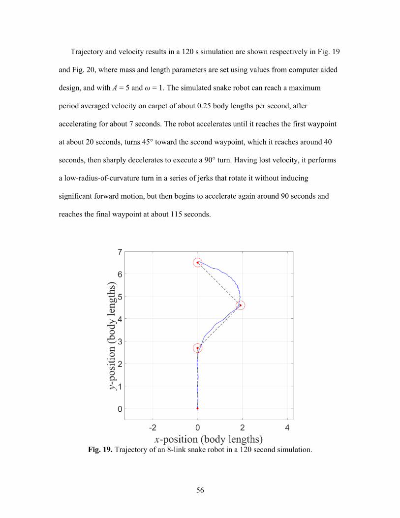
Trajectory and velocity results in a 120 s simulation are shown respectively in Fig. 19
and Fig. 20, where mass and length parameters are set using values from computer aided
design, and with A = 5 and ω = 1. The simulated snake robot can reach a maximum
period averaged velocity on carpet of about 0.25 body lengths per second, after
accelerating for about 7 seconds. The robot accelerates until it reaches the first waypoint
at about 20 seconds, turns 45° toward the second waypoint, which it reaches around 40
seconds, then sharply decelerates to execute a 90° turn. Having lost velocity, it performs
a low-radius-of-curvature turn in a series of jerks that rotate it without inducing
significant forward motion, but then begins to accelerate again around 90 seconds and
reaches the final waypoint at about 115 seconds.
Fig. 19. Trajectory of an 8-link snake robot in a 120 second simulation.
57
Fig. 20. Forward speed of an 8-link snake robot in a 120 second simulation.
Using the MBD model of [49], we tested the effect of increased articulation in a two-
DOF snake by comparing the simulated steady-state speed of a three-link snake with a
snake composed of two, four-link coupled linkages. The two simulated snakes were of
equal body length and both applied (28), with identical control parameters. The results of
this simulation experiment, displayed in Fig. 21, indicate that the more highly articulated
snake outperforms the three-link snake across all combinations of tested control
parameters.
58
Fig. 21. Simulated steady-state speeds of two 2-DOF snake robots, one with three links (dotted line) and one with eight (solid line), as a and ω are varied.
6.2. Feedback Linearization
As discussed in Sec. 5.3, an N-link snake robot moving in the plane can be modeled in a
multibody dynamic approach as a serial chain of straight links joined by revolute joints,
with 3N DAEs per link and 2(N–1) per revolute constraint. The global position of the ith
link CM is specified by a vector of generalized coordinates qi = [ri,ϕi]T, where ri = [xi,yi] is
the global position of the ith link in the xy-plane and ϕi is its global orientation. Defining a
vector of Lagrange multipliers λi = [λx,i, λy,i]T, a diagonal 3×3 generalized mass matrix Mi,
a generalized external force vector Fext,i, and a vector of generalized actuation forces Ui for
the ith link, the system’s equations of motion may be written in the form
( )( ) ( )
ext, 1
1 1 1 1 1
, ,
, , , , , ,i i i i i i i
j j j j j j j j j j
φ
φ φ φ φ φ φ φ φ−
+ + + + +
⎧ = + +⎪⎨
− = +⎪⎩
M q F f λ λ U
r r g h (29)
59
(i ϵ N and j ϵ N–1), where f, g, and h are vector valued functions that account for the
mechanism’s internal forces. Note that since joint torques are the only control inputs, only
the angular components of Ui are nonzero: Ui = [0, 0, Ui]T.
Thus, as was observed in [50], the angular coordinates of a snake robot can be linearized
by setting Ui = Ui,lin + Ūi, where Ūi is set to track (4) and Ui,lin is set to cancel undesirable
forces, in this case the angular components of Fext,i and f. Solving a system of 4N–2
equations for all of the λi, each of the Ui,lin may be written as functions of the generalized
coordinates and their derivatives.
The MBD model described above can be modified to represent a snake robot composed
of the coupled linkages described in Sec. 4.2 by including the cable equations given by (2).
The linearizing control input Ui,lin at each joint can in this case be determined in exactly
the same way as described above, but the system lacks sufficient DOFs to simultaneously
apply these torques at each joint. We therefore take the following approach: the output τM
of the controller in (28) is input to a function M→J, which determines the effect of a motor
torque on each of the mechanism’s joints. A feedback linearization is then performed
exactly as before, outputting a linearizing control torque Ui at each joint. Since by (2) the
joint torques are all linear with the motor torque, the Ui can then be input to a function
J→M, which solves the cable equations backwards to determine the torque that would be
induced at the motor by each of the desired joint torques, and sums these values. The
resulting “best case” linearized motor torque τM,ℓ is the motor torque that cancels the
greatest possible fraction of the nonlinearities at each of the joints, since it is effectively an
average over the linearizing joint torques. This method was tested in simulation in a snake
robot composed of two 4-link bending modules, where estimates of the external forces
60
were input to each of the Fext,i and λi. As shown in Fig. 22, feedback linearization increased
the maximum achievable steady-state speed for all force estimates between 0% and 100%
of the true values, with a maximum increase of between 15.5% and 27.5% for perfect force
estimates.
6.3. Path Following
A snake robot driving its joint angles according to (8) moves in a straight line for θ0 =
0 and at constant radius of curvature for constant, nonzero θ0 [24]. In Liljebäck et al. [38],
a path following controller is defined by setting
( )0 refhA h hθ = − (30)
where the heading 1
11
N
ii
hN
θ=
=− ∑
is the average joint angle, Ah is a constant gain, and href is
the desired heading, defined as
Fig. 22. Steady-state speed for a 2-module snake robot as estimates of external forces are varied between 0% and 140% percent of the actual values.
61
ref Xarctan( / )h P= − Δ (31)
where the “cross track error” PX is the shortest distance from the snake’s CM to the desired
path and Δ is the constant “look-ahead distance.”
Alternatively, the cross track error for the ith link and jth waypoint may be defined as
( ) ( )222 2 2 2x, , 1 , 1 ,2ij i j j i j i j jp K E K K E
−
− −= − − + (32)
where Ki,j is the distance from the ith link frame to the jth waypoint and Ej is the distance
between the (j–1)th and jth waypoints. A single cross track error px,j may then be defined
as a weighted average over the links. Defining vij = [vij,x vij,y]T as the vector from the ith link
frame to the current waypoint and wj = [wj,x wj,y]T as the vector between the current
waypoint and the previous waypoint, a signed cross track error may be defined as PX,j = –
sgn(θrel – θwp)px,j, where
, ,rel wp
, ,
arctan , arctanij x j x
ij y j y
v wv w
θ θ⎛ ⎞ ⎛ ⎞
= =⎜ ⎟ ⎜ ⎟⎜ ⎟ ⎜ ⎟⎝ ⎠ ⎝ ⎠
(33)
Here, the signum function determines which side of the desired path the robot is on. The
angle between desired paths θwp is also used to ensure that when switching paths the robot
always turns through the smaller angle between paths. In place of (31), the desired heading
for the jth waypoint is set according to
( )ref X, X, X, wp0arctan
t
h j h j h jh P P I P dt D P θʹ′= − + + +∫ (34)
The integral term in (34) acts to compensate for steady state error in the distance of the
snake robot from the desired path, under large disturbance forces due, for example, to
obstacles, water currents, or gravitational forces. Special care must be taken to avoid
instabilities in the integral term under large errors, and in particular during the transient
62
states when the snake is switching targets. Thus, if either the cross track error PX or the
heading error |θrel–θwp| pass some maximum values, the integral term is reset to zero. The
heading gains must also obey the condition Ih/Ph < H for a constant H, to prevent the snake
from banking too hard. Fig. 23 displays a comparison of path-following errors with and
without the integral term, for a 3-link, full-DOF snake following the line x = 0, under a
constant disturbance in the positive x-direction. The link length Li is taken to be a constant
L for all i, and the position of the robot’s “head” (the end of its first link) is plotted in units
of L.
Fig. 23. Path following under a disturbance
63
We can modify the controller further by setting ℎ123 = – arctan 𝑃v𝑃w,x +
𝐼v arctan 𝑃w,x𝑑𝑡yXY + 𝜙/, so that, in the spirit of the full controller, the integral term
avoids instability with the use of an arctangent function. Defining ϕAoA to run from 0° to
180° on one side of the path and from 0° to –180° on the other, the controller can be
improved by setting Ph = p1(arctan2(p2 ϕAoA)+p3), where p1, p2, and p3 are gains, so that the
snake more aggressively approaches the desired path when the heading error is large. This
definition of the heading gain ramps down the cross-track error correction as the snake
approaches the correct heading in order to cause a smooth approach to the desired path.
This approach was observed to increase the speed of a snake following a series of paths in
simulation, essentially by decreasing path overshoot.
6.4. Simulation Study 1: Phase Offset Optimization
A reduced-DOF snake with Nb bending modules of N links each has the same number
of DOFs as a full-DOF snake with (Nb+1) links, but a structure similar to a full-DOF snake
with NbN links. We thus conjecture that the δopt that maximizes steady state speed in a
reduced-DOF snake will fall between the optimal values for these two cases.
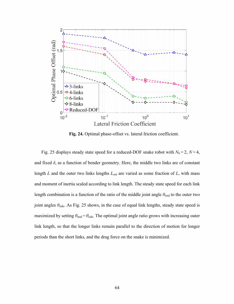
Fig. 24 displays δopt for full-DOF snake robots of various length, as cn in (15) is varied,
and where ct = 0. The values of δopt for a reduced-DOF snake with equal link lengths, with
Nb = 2 and N = 4, are also displayed, and as expected, remain between the corresponding
values for the 3-link case and the 8-link case. Unlike the prediction given by (9), δopt
depends on cn in simulation. The results differ most sharply in the case of very low friction,
where slipping is most pronounced. Note that δopt is undefined for cn = 0.
64
Fig. 24. Optimal phase-offset vs. lateral friction coefficient.
Fig. 25 displays steady state speed for a reduced-DOF snake robot with Nb = 2, N = 4,
and fixed δ, as a function of bender geometry. Here, the middle two links are of constant
length L and the outer two links lengths Lout are varied as some fraction of L, with mass
and moment of inertia scaled according to link length. The steady state speed for each link
length combination is a function of the ratio of the middle joint angle θmid to the outer two
joint angles θside. As Fig. 25 shows, in the case of equal link lengths, steady state speed is
maximized by setting θmid = θside. The optimal joint angle ratio grows with increasing outer
link length, so that the longer links remain parallel to the direction of motion for longer
periods than the short links, and the drag force on the snake is minimized.
65
Fig. 25. Steady state speed vs. joint angle ratio.
6.5. Force Control and Obstacle Interaction
When the base of a bending module is fixed with respect to an external object, and under
the assumption of static equilibrium, the torque acting on each joint is related to its angular
displacement by a simple application of Hooke’s Law. The joint torques τ = [τi, …, τN–1]T
can then be written in terms of the net force Fe = [Fe,x, Fe,y]T applied by the end effector (the
last link of the module) as τ = JT(R0e)TFe, where J is the module’s Jacobian and R0e is the
rotation matrix from the base frame to the end effector frame. Multiplying this equation by
the pseudoinverse of JT, the end effector force can be written as a function of the joint
torques: Fe = R0e(JJT)–1Jτ, where τ is given in terms of the pulley angular displacement ΔθP
by (1). Numerically solving the two resulting transcendental equations for the two
components of Fe, ΔθP can in general be written as a function of Fx or Fy. Since the
66
mechanism has only a single DOF, either component of Fe, but not both, can be controlled
by controlling ΔθP, sufficient for pushing off of or grasping external objects.
Adaptation to obstacles can be handled by adding an obstacle offset 𝜃Uz{ =
𝑘Uz{ 𝑐+V|–:+@: 𝑒+ to θ0, where kobs is a gain, ei is the obstacle induced displacement in the
ith joint, and ci is the joint weighting defined in Sec. 6.1. Here, we set ei as the ith joint
displacement measured by the rotary position sensor minus the angle predicted for this
joint by the kinematic constraints in (1), for a pulley angle θP. This definition is essentially
an application to an underactuated mechanism of the principle outlined in [51] and [52],
where a snake robot is able to slide around obstacles by applying a control torque
proportional to a power of obstacle-induced curvature. Alternately, we can accomplish the
same effect without reference to pulley angle by comparing every joint to every other joint.
There are 𝑁–12 combinations of joints, so we set θobs = –kobsε, where
( )1 1
1 1
2( 1)( 2)
N Ni ij jj i jC
N Nε θ θ
− −
= = += −
− − ∑ ∑ (35)
and where 𝐶+x =
1�–1�–�1�–1�–�
relates the ith and jth joints. Notice that, due to the SEAs, the
application of a control torque of this form results in an equivalent spring force between
the snake and an obstacle. The curvature controller and obstacle offset together constitute
an impedance controller, which acts in parallel with the more local obstacle interaction
behavior described in Sec. 4.3.
A block diagram of the full control algorithm for the snake robot is displayed in Fig.
26. In overview, the heading offset θ0 is set according to a path-following controller and
modified by an obstacle offset, and is then input to the “curvature controller,” which
determines the desired motor torque τM in order to bend the module sinusoidally, taking
67
as feedback the present positions of each of the joints. The resulting torque output is then
modified by the partial feedback linearization block, which attempts to cancel the greatest
possible portion of the nonlinear forces internal to the mechanism, and outputs a final,
linearized motor torque τM,ℓ at the pulley. In the diagram, “Lin.” represents the feedback
linearization and “Force est.” is an estimation of external frictional forces, consisting in
this case of a viscous frictional model. In simulation, the force estimator was usually set
to output a given percentage of the actual frictional forces, and the actual frictional forces
were (optionally) overlaid with a Gaussian noise term.
Fig. 26. The complete control scheme for the cable-driven snake robot.
68
CHAPTER 7
USE AS A MODULAR RECONFIGURABLE PLATFORM
7.1. Inchworm Locomotion
In an S cable routing scheme, where cables are alternately routed on the left and right
sides of a link, the amount by which a segment rotates relative to the segment beneath it is
given by a modification of (1): P( 1)ii iθ α θ= − , with the same definition of αi, so ensuring
that ri/Di–ri–1/Di–1 is constant for all i guarantees that every other joint angle is equal and
opposite, and the module will form an S-shape. A single module can thus approximate an
entire period of a sinusoid. However, single-DOF slithering locomotion is not possible with
this configuration, since there is no phase difference in the propagation of the sine wave
along the length of the module, and the propulsive force averaged over an oscillation period
is zero. However, S-routing can be used for single-module, inchworm like locomotion.
We can calculate the propulsive force contributed by the ith link during the downward
phase of its motion by solving the transcendental equation Li–1sinϕi–1 = Lisinϕi, where we
take ϕi – ϕi–1 = Asin(ωt) for all i. Assuming equal half-link lengths L, this equation may be
solved exactly, so that cos(ϕi) = |sin(Asin(ωt))|. The net propulsive force is then given by
( )( )( )4
sin sinnet f bNF c tc ALτ
ω= − (36)
where N is the number of links in the mechanism, τ is the torque applied at each joint, and
cf and cb are the coefficients of friction for forward and backward motion, respectively.
69
7.2. Three Dimensional Motions
The rigid structure of each Planar Bender module allows for rotation about the axis
which runs along the length of its body (which we call the z-axis) without a change in
bending due to coupling or sagging. Thus, a rolling motion of a bender about the z-axis by
an angle Θ transforms the local coordinate frame by Rz,Θ, the rotation matrix about the z-
axis for that angle.
The Planar Bender is designed for both planar maneuvers and spatial maneuvers in
conjunction with a rotational unit. Including a pure rolling-DOF departs from the biological
design, and may allow for the use of gaits not found in nature. A gait similar to sidewinding,
where bending sections are progressively lifted and placed down, should also be possible.
Performing three-dimensional movements will require precise coordination of the bending-
DOF with the rolling-DOF, making it necessary to understand how the dynamics of the
bending mechanism, and particularly its moments of inertia, change as it bends. A
representation of the mechanism, with variables used in the below moment of inertia
calculations, is displayed below.
We define the y-axis as the axis perpendicular to the plane of bending and the z-axis
as the one about which the rolling-DOF acts (referring to Fig. 1), and we define IY,i and
IZ,i as the moments of inertia of the ith link about these respective axes. Modeling the
links as thin rods, the y-axis moments of inertia may be computed recursively as IY,i =
miλi,y2+mihi
2/12, where λi,y = [Λi–12+ (hi/2)2–Λi–1hicos(ψi–1)]½ is the distance from the
origin to the ith link center and Λi = [Λi–12+hi
2–2Λi–1hicos(ψi–1)]½ is the distance from the
origin to the ith joint. We define the angle ψi = θi–αi, where αi = arcsin[(hi-1/Λi)sin(ψi–1)],
and ψ1 = θ1.
70
Fig. 27. Position and forward speed of an 8-link snake robot.
The z-axis moment of inertia may be modeled by treating each of the links as a solid
cylinder of radius li, height hi, and mass Mi. Employing moment of inertia tensor
transformations, IZ,i = ½(Iz,i+Ix,i)+½(Iz,i–Ix,i)cos(2θi), where Iz,i = ½Mili2 is the moment of
inertia of each cylinder about its axis and Ix,i = (Mi /hi)[li2(hi–λi,z)/4+(hi–λi,z)3/ 3] is the
moment of inertia of each cylinder about a line normal to its surface and passing through
its base. Here, Ix,i is given by the relation λi,z = Σik=2|hk–1sin(θk–1)|. The above expressions
for Iy and Iz were computed numerically, where Mi, hi, li, and θi were taken to be constant
for all i. Fig. 28 displays the results of these calculations, normalized by the moments of
inertia of the first link, as the angle of the first joint moves from –60° to 60°.
71
1.6
1.4
1.2
1.0
0.8
θ1 (deg) Fig. 28. Modeled Moments of Inertia of the Bending Module
7.3. Tripedal Configuration
Three benders may be arranged together at angular displacements of γ = 120º to form
a Triped Robot. Since each leg is restricted to a planar bending motion, the other two legs
are entirely responsible for stabilizing the motion of that leg perpendicular to this plane.
Thus, we may write a s-tability controller in three parts, in which each of the legs is
stabilized separately. For each leg, we draw a plane perpendicular to the leg’s plane of
bending, onto which we project the other two legs, and control the orientation of the legs
within that plane. The relative angles between benders are fixed, so the projection of a
bender into the plane is given by multiplying its position in its own bending plane by the
rotation matrix sin( / 2) 00 1
Rγγ⎡ ⎤
= ⎢ ⎥⎣ ⎦
. Multiply by the inverse matrix Rγ–1 to transform back
into the frame of the bender. A feedforward term may be calculated by counteracting the
torque that gravity applies on the feet at a given configuration. A PD control law is then
72
applied to maintain the foot orientations αi at the desired values. The foot orientation is
calculated using the IMU in the head. Locomotion may be achieved by varying the αi
sinusoidally:
( ), sin( ) sin(i ref i i i iA t tα ω ϕ ω ϕ δ= + + + − (37)
Setting φ2 – φ1 = π and φ2 = φ3 results in a gait in which a “front leg” and two
synchronized “back legs” take turns stepping forward and standing in place. By tuning the
values of the amplitudes Ai and offsets δi, a crawling gait may be achieved, in which the
front leg moves through a large displacement to provide the primary source of propulsion,
while the back legs act as stabilizers, or alternately, two legs propel while one stabilizes.
During this motion, all of the feet always maintain contact with the ground, so locomotion
requires anisotropic friction on the feet. For this purpose, wedge shaped adapter pieces
were designed, which can connect to a bender module via the male-female interface.
Tipping is prevented by ensuring that the center of mass (CM) remains inside the
robot’s support polygon. As in the above controller, we can simplify the situation by
separately viewing the projections of the robot onto the planes perpendicular to each of the
three legs. Preventing tipping than reduces to constraining each of the projections of the
CM to remain on the “support line” in between each of the three pairs of adjacent legs. If
the projection of the CM in a particular plane approaches one of the feet, a “tipping
controller” acts on the leg so that its projection on that plane extends, reestablishing a stable
configuration.
The control action can be made to be continuous by giving the tipping controller the
form of a potential well: τmin = a(x–xmin)–b and τmax = a(x–xmax)–b up to the maximum torque,
after which point the controller continues to apply its maximum value. Note that we have
73
defined positive torque to correspond to inward bending of the leg. Tuning the parameters
a and b, the potential well can be made arbitrarily steep, to prevent interference with the
action of the controller in (37). Each leg applies one τmin and τmax, corresponding to the
other two legs, so there are six total tipping controllers.
A multibody dynamic model of one such planar projection was used to validate the
stability controller, the crawling gait given by (37), and the tipping controller. In this
model, ground was treated as a series of stiff spring dampers, which apply forces at each
CM, and forces and torques at each link end. The simulated planar robot succeeded in (a)
raising itself from a flat configuration to a standing position, (b) maintaining a standing
position using the stability controller, c) crawling forward, and (d) smoothly lowering itself
to the ground from a standing position. One of the advantages of this design is that the
robot is symmetric with respect to the bending planes of its three legs. Thus, directional
changes can be accomplished without any manipulation of leg orientation by simply
changing which leg acts as the front leg.
74
CHAPTER 8
EXPERIMENTAL SETUP AND RESULTS
This section presents the results of experimental studies of force control, locomotion,
and obstacle interaction in the snake robot prototype introduced in Sec. 4.1.
8.1. Force Control
The force controller described in Sec. 6.6 was tested in a single module in two
configurations, θ1 = 0° and θ1 = 30°, for three desired force outputs, 10 N, 15 N, and 20 N.
A single module was placed horizontally, so that gravitational effects could be ignored,
and allowed to reach the desired configuration unimpeded. The last link of the module was
then placed parallel to an MLP-25 compression load cell rated for 44.5 N, and the module’s
base was fixed to ground. At θ1 = 0° and 10 N desired force, the model in Sec. 6.6 predicts
a required pulley angular displacement of ΔθP = 35.3°. In practice, ΔθP had to be adjusted
approximately 6% above this value to achieve the desired force output, possibly as a result
of frictional effects or errors in the kinematic constraints. This correction multiplier was
held constant in all subsequent experiments. In accordance with the model in Sec. 6.6, in
the θ1 = 30° configuration, the robot commands a ΔθP approximately 1.4 times the value
required for the θ1 = 0° case. The results of these experiments are shown in Fig. 29, after
application of a locally weighted linear regression smoothing. Note that the load cell used
in these experiments has a settling time of over a second, which causes the force
measurements to decrease slightly after the applied force has plateaued. The results in Fig.
29 demonstrate that the bending module is able to successfully control the perpendicular
75
component of the end effector force by controlling the pulley’s angular position, with less
than 5% error in all but one of the six trials.
Fig. 29. Force control experiments for (A) Straight configuration (θ1 = 0°) and (B) Curved configuration (θ1 = 30°).
76
8.2. Locomotion and Steering
As discussed in [49], the controller outlined in Fig. 27 was tested in simulation using the
MBD model from Sec. 6.6. In the prototype, the feedback linearization is removed, the
path follower is replaced by manual steering, and the output of the controller is cascaded
into the servomotor’s internal PID loop.
Planar locomotion and steering were tested in the prototype by tracking its trajectory
on floor tiles over roughly four periods of oscillation, starting from a straight configuration
and with α = 2.45 rad, δ = 1.27 rad, and ω = 3.77 Hz. The front link of the snake was labeled
with a blue marker and the back link with a red marker, as shown in the snapshots in Fig.
30. (Locomotion seems to be more effective when the “head” module is dragged behind
the snake rather than pushed ahead of it.)
A 12.3 megapixel camera positioned at a height of approximately two meters and facing
the ground was used to record the motion of the snake. These videos were sampled at 10
Hz and scaled using the known dimensions of the tiles, after which the centroids of each
marker were tracked. The resulting trajectories are shown in Fig. 31, for values of θ0
between –0.15 rad and 0.15 rad.
The prototype is capable of traveling at speeds of about 0.07 body lengths per second,
comparable to the speed of serpentine locomotion in some large biological snakes [53], but
more than an order of magnitude slower than the fastest snakes [4]. The prototype appears
to have a slight bias to the left and exhibits higher amplitude oscillations during right
turning than left turning, most likely on account of asymmetries in the cable constraints.
However, an orientation offset of this size can also occur in simulation due to initial
conditions, and is easily corrected by actively controlling θ0.
77
(A) (B)
Fig. 30. Snapshots of the snake robot executing a counterclockwise turn, showing a half period of oscillation between (A) and (B). The black marker in the top left corner provides a point of reference.
Fig. 31. Trajectories of the front link of the snake robot over approximately four oscillation periods, for various values of θ0. (Positive values correspond to clockwise turning).
78
8.3. Obstacle Interaction
The obstacle interaction procedure of (35) was tested experimentally by recording the
trajectory of the snake robot as it moved past a circular, 5 kg cast iron plate, with a radius
of approximately 8 cm. The robot was started in a straight configuration, flush with the
obstacle and tangent to it, at an angle of approximately 45° from the global y-axis. The
robot was then commanded to move forward, with θ0 = 0 and the other controller
parameters set at the same values as in the locomotion experiment in Sec. 8.2. The
experiment was repeated for three values of kobs, the results of which are displayed in Fig.
32. In these experiments, the front and back of the snake are tracked as in Sec. 8.2 and the
angle that the vector between the red and blue markers forms with the global y-axis is taken
as a good approximation for the snake’s global orientation. The initial and period-averaged
final orientations of the snake are denoted in the figure by arrows.
Without the controller in (35) (i.e. kobs = 0), the snake is observed to rotate about the
obstacle by the following process. The front module contacts the obstacle first and induces
a moment about the snake’s CM that rotates the robot away from the obstacle. However,
this movement brings the back module into contact with the obstacle, and a moment is then
induced in the opposite direction. At this point, for an obstacle of this size, the front module
has moved past the obstacle and only the back module continues to contact it. The snake is
then progressively rotated, but the curvature of its trajectory is low enough that the point
of contact with the obstacle moves down the length of the back module until the snake
eventually loses contact with the obstacle and moves past it.
Thus, two competing tendencies determine the amount of rotation induced by an
obstacle: the magnitude of the moment produced by each impact and the amount by which
79
the point of contact moves down the length of the snake between impacts. In the experiment
in Fig. 32, the case kobs = 0 results in about a 168° change in orientation before contact with
the obstacle is lost. Increasing kobs to 1.33, the snake tends to bend more in the direction of
contact, resulting in an orientation change of about 221° over the same period. On the other
hand, a negative value of kobs effectively offsets obstacle induced rotation by rotating the
reference heading in the opposite direction. The snake can thus be made to push off or
continue past an obstacle, as in the case kobs = –2 in the figure, where the snake continues
on with little change to its initial heading (only about 17°). Note however, that this behavior
is highly dependent on the size and shape of the obstacle.
Fig. 32. Trajectories of the back link of the snake robot during interaction with a circular obstacle. Initial position is denoted by two concentric circles at (0,0).
80
CHAPTER 9
CONCLUSION & FUTURE WORK
9.1. Summary
This paper presented the development of a cable-driven snake robot with coupled
joints, which incorporates series elastic elements as a means of producing automatic
obstacle interaction behavior. A simplified model of serpentine locomotion was developed
and used to analyze how the locomotive efficiency of a snake robot is related to the number
of links it contains. A control scheme was devised for a snake robot comprised of coupled
linkages and combined with a feedback linearization of the joint dynamics. These ideas
were tested in simulation studies and experiments with a prototype.
9.2. Future Work
Whereas the cable-actuated module presented in this paper can approximate planar
curvature profiles, the antagonistic cable routing scheme of the present design is not well
suited to three-dimensional motions. With more sophisticated cable routing, additional
DOFs may be possible in a single module, enabling more natural and versatile locomotion.
The use of the bending module as a modular reconfigurable robotic platform is also being
explored, and a second “spinner” module, which allows for rotation of the snake about its
principal axis, has been designed to allow for three-dimensional motions such as
sidewinding. Decoupled “bending” and “spinning” degrees of freedom do not exist in
biological snakes and may facilitate locomotion gaits not found in nature.
81
REFERENCES
[1] S. Hirose, “Biologically Inspired Robots (Snake-like Locomotors and
Manipulators),” Oxford Univ. Press, 1993.
[2] P. Liljebäck, K. Y. Pettersen, Ø. Stavdahl, and J. T. Gravdahl, “Fundamental