124
DESIGN AND DEVELOPMENT OF AN EMBEDDED CONTROL SYSTEM FOR CONTROLLING A DC MOTOR USING MICROCONTROLLER MOHAMAD REZDUAN BIN MOHD JAN B050810149 UNIVERSITI TEKNIKAL MALAYSIA MELAKA 2011
| Date post: | 04-Aug-2019 |
| Category: |
Documents |
| Upload: | hoangduong |
| View: | 215 times |
| Download: | 0 times |
DESIGN AND DEVELOPMENT OF AN EMBEDDED CONTROL SYSTEM FOR CONTROLLING A DC MOTOR
USING MICROCONTROLLER
MOHAMAD REZDUAN BIN MOHD JAN
B050810149
UNIVERSITI TEKNIKAL MALAYSIA MELAKA
2011
UNIVERSITI TEKNIKAL MALAYSIA MELAKA
DESIGN AND DEVELOPMENT OF EMBEDDED CONTROL
SYSTEM FOR CONTROLLING A DC MOTOR USING
MICROCONTROLLER
This report submitted in accordance with requirement of the Universiti Teknikal
Malaysia Melaka (UTeM) for Bachelor Degree of Manufacturing Engineering
(Robotic and Automation) with Honours.
by
MOHAMAD REZDUAN BIN MOHD JAN
B050810149
FACULTY OF MANUFACTURING ENGINEERING
2011

UNIVERSITI TEKNIKAL MALAYSIA MELAKA
BORANG PENGESAHAN STATUS LAPORAN PROJEK SARJANA MUDA
TAJUK: Design And Development Of An Embedded Control System For Controlling A DC
Motor Using Microcontroller
SESI PENGAJIAN: 2010/2011 Semester 2 Saya MOHAMAD REZDUAN BIN MOHD JAN mengaku membenarkan laporan PSM ini disimpan di Perpustakaan Universiti Teknikal Malaysia Melaka (UTeM) dengan syarat-syarat kegunaan seperti berikut:
1. Laporan PSM / tesis adalah hak milik Universiti Teknikal Malaysia Melaka dan penulis.
2. Perpustakaan Universiti Teknikal Malaysia Melaka dibenarkan membuat salinan untuk tujuan pengajian sahaja dengan izin penulis.
3. Perpustakaan dibenarkan membuat salinan laporan PSM / tesis ini sebagai bahan pertukaran antara institusi pengajian tinggi.
4. *Sila tandakan (√)
SULIT
TERHAD
⁄ TIDAK TERHAD
(Mengandungi maklumat yang berdarjah keselamatan atau kepentingan Malaysia yang termaktub di dalam AKTA RAHSIA RASMI
1972)
(Mengandungi maklumat TERHAD yang telah ditentukan oleh
organisasi/badan di mana penyelidikan dijalankan)
Alamat Tetap :
Kampung Sawah Raja
71350 Kota
Negeri Sembilan Darul Khusus
Tarikh: _______________________
Cop Rasmi:
Tarikh: _______________________
* Jika laporan PSM ini SULIT atau TERHAD, sila lampirkan surat daripada pihak organisasi berkenaan dengan menyatakan sekali sebab dan tempoh tesis ini perlu dikelaskan sebagai SULIT atau TERHAD.
DECLARATION
I hereby declared this report entitled “Design And Development Of An Embedded
Control System For Controlling A DC Motor Using A Microcontroller’’ is the
result of my own research except as cited in the references.
Signature : ………………………………………………..
Author’s Name : MOHAMAD REZDUAN BIN MOHD JAN
Date : 19 MAY 2011
APPROVAL
This report is submitted to the Faculty of Manufacturing Engineering of UTeM as a
partial fulfillment of the requirements for the degree of Bachelor of Manufacturing
Engineering (Robotic and Automation) with Honours. The members of the
supervisory committee are as follow:
(Signature of Supervisor)
………………………………………
(MOHD NAZRIN BIN MUHAMMAD)
(Official Stamp of Supervisor)
i
ABSTRAK
Dalam era teknologi yang moden ini, sebuah sistem elektrik banyak digunakan dalam
bahagian elektrik dan elektronik untuk melakukan aplikasi-aplikasi tertentu. Ini adalah
sistem yang dibina untuk menyelesaikan dan mengendalikan aplikasi-aplikasi tertentu.
Tujuan utama projek ini adalah untuk merancang dan mengembangkan suatu sistem
kawalan litar tertanam untuk mengendalikan motor dc menggunakan pengawal mikro.
Sebuah sistem tertanam terdiri daripada tiga elemen penting. Salah satu elemen ini ialah
mereka sebuah litar. Seterusnya adalah pembangunan dari bahagian kawalan. Untuk
projek ini, pengawal mikro dipilih kerana arahan berulang boleh digunakan di dalam
pengawal mikro. Untuk mengawal motor arus terus, sebuah elemen dari sistem kawalan
PID digunakan. Sistem kawalan PID terdiri daripada Kp, Ki and Kd. Setiap komponen
mempunyai tugasnya tersendiri. Kp digunakan untuk meningkatkan tindak balas dalam
sesuatu sistem. Nilai untuk Kp boleh diubah untuk mendapat nilai optimum tindak balas
dalam sesuatu sistem. Ki pula digunakan untuk mengatasi masalah keadaan mantap.
Untuk Kd pula, ia digunakan untuk mendapatkan suatu keadaan yang tepat. Dengan
menggunakan PID ini, ubahsuai boleh dilakukan di dalam aturcara untuk mendapatkan
suatu kedudukan yang tepat dan betul. Nilai PID ini digunakan untuk meningkatkan
tindak balas dan mengurangkan kesalahan dalam sesuatu sistem. Semua maklumat yang
berkaitan tentang kaedah untuk mengawal motor arus terus juga telah dibincangkan
dalam projek ini.
ii
ABSTRACT
In this modern era technology, an embedded system is widely used in most electric and
electronic component for specific task. It is simple systems that are built up for
accomplish and control specific task. The main purpose of this project is to design and
developed an embedded an embedded control system for controlling a dc motor using a
microcontroller. An embedded system consist three important elements during the
development. One of the elements is designing a hardware that consist a schematic
diagram. Next is the development of the control part. For this project, microcontroller
was selected because of the repeated instruction can be used inside the microcontroller.
For controlling a dc motor, an element of the control system were added which is PID
algorithm. PID algorithm consist three components which is Kp, Ki and Kd. Each
component has their own capability for controlling a dc motor. Kp can be used for
increase the transient response of dc motor. We can set some values of Kp until get a an
optimum system response. For the Ki, it was used for overcome the steady state error.
Lastly, Kd is used to get a better response in achieving a set point of the controller by
entering a value. By using a PID algorithm, adjusting can be easier by set up in the
programming section and the real position of rotation dc motor will get through this
programming. This PID algorithm will increase the transient response and reduced the
steady state error that exists in the system.

iii
DEDICATION
Firstly, thanks to Allah S.W.T with his blessing, I have done in completing my final year
project with succeed. I would apply my gratitude to my father Hj Mohd Jan Bin Udin and
my mother Hjh Siti Rahmah Binti Ahmad for giving me a supporting to complete this
project. They encourage and inspire me through this project and completing this report.
This report is dedicated to my parents of blessed memory, who raise me to be a
responsible and careful person. Other than that, I would like to thank to everyone for
supporting me in this project.

iv
ACKNOWLEDGEMENT
Assalamualaikum Warahmatullahi Wabarakatuhu. Alhamdulillah, thanks to Allah S.W.T.
because with his blessing I have done this final year project with succeed and without any
obstacles.
First and foremost I would like to take this opportunity to express my highest gratitude
and appreciation to my supervisor, Mr. Mohd Nazrin Bin Muhammad who gives me a
spirit and motivation, an opinion to make me feel comfortable and more confident in
completed this final year project. He also encourages me in knowing the real thing on
how to be a good engineer. The tips that he gives to me, it will not be forgotten and I will
work hard until I get succeed.
Other than that, thanks to all my friends for help and giving some opinion to me in
accomplish this final year project.
v
TABLE OF CONTENTS
Abstrak . I
Abstract ii
Dedication iii
Acknowledgement iv
Table Of Contents v
List Of Tables ix
List Of Figures x
List Of Abbreviations xii
1. INTRODUCTION 1
1.1 Problem Statement 4
1.2 Objective 4
1.3 Scope 5
1.4 Limitation of the project 6
1.5 Project outline 6
1.6 Expected outcome 7
1.7 Conclusion 7
2. LITERATURE REVIEW 10
2.1 Historical of an embedded system 10
2.2 Definition of an embedded system 12
2.3 Characteristic and reliability of embedded systems 13
2.4 Purpose of embedded systems 14
2.4.1 Data collection and storage representation 14
2.4.2 Data communication 15
2.4.3 Data signal processing 15
2.5 Design and development of an embedded system 16
vi
2.5.1 Schematic design 17
2.6 Control system element 19
2.6.1 PID definition and element 21
2.6.2 PID application 23
2.6.3 PI speed controller 27
2.7 Controller in embedded system 28
2.7.1 Microcontroller definition 29
2.7.2 Microcontroller application 30
2.8 Method for controlling a dc motor 32
2.8.1 Controlling using Pulse Width Modulator 34
2.8.2 Controlling using H-Bridge 38
2.9 Conclusion 43
3. METHODOLOGY 44
3.1 Flow chart 45
3.2 Design and development 46
3.2.1 Hardware development 47
3.2.2 Programming section 47
3.2.3 PID for Control System 48
3.2.3.1 Proportional Controller 49
3.2.3.2 Integral Controller 51
3.2.3.3 Derivative Controller 52
3.2.3.4 PID Controller 53
3.3 Testing 54
3.4 Interfacing using USB UART 55
3.5 Block diagram 56
3.5.1 Computation of error signal and PID compensation algorithm 56
vii
4. DESIGN AND DEVELOPMENT 57
4.1 Flow chart 57
4.2 Schematic design 60
4.2.1 Procedure for schematic design 60
4.3 PCB layout 62
4.3.1 Procedure for PCB layout design 62
4.4 Hardware development 64
4.4.1 Procedure for etching process 64
4.4.2 Procedure for soldering process 65
4.4.3 Finish hardware development 66
4.5 Designing PID controller 67
4.6 Programming section 69
4.6.1 Servo calculation 69
4.6.1.1 Position updates 70
4.6.1.2 Error calculation 70
4.6.1.3 Trajectory updates 71
4.6.1.4 Duty cycle calculation 72
4.6.1.5 Procedure for programming section 73
4.6.1.6 Command interpreter 74
4.6.1.7 Stand alone operation 75
5. RESULT AND DISCUSSION 76
5.1 Result 76
5.2 Completed design of an embedded system 77
5.2.1 Circuit description 77
5.3 PID controller 78
5.3.1 Block diagram for PID controller 78
5.3.2 Uncompensated system 79
viii
5.3.3 PD compensated system 83
5.3.4 PI compensated system 88
5.4 Interface section 92
5.4.1 Procedure during interfacing 92
5.5 Database result 94
5.6 Conclusion and finding 97
6. CONCLUSION AND RECOMMENDATION 98
6.1 Conclusion 98
6.2 Recommendation and future work 99
REFERENCES 101
APPENDICES 103
ix
LIST OF TABLES
1.1 PSM 1 table 8
1.2 PSM 2 table 9
5.1 Theorytical value of distance 94
5.2 Actual value without using PID 94
5.3 Actual value for PID using 100mm/s velocity 96
5.4 Actual value for PID using 200mm/s velocity 96
x
LIST OF FIGURES
1.1 Embedded system 3
2.1 Flow chart for designing a circuit 16
2.2 Schematic circuit 18
2.3 Simplified description of a control system 19
2.4 Closed loop control system 20
2.5 PID controller works 24
2.6 Error speed as a function of reference speed for different
Ki values with Kp 25
2.7 Comparison of transient performance for different control
Algorithm 26
2.8 Microcontroller 31
2.9 Brush Dc Motor 33
2.10 PWM signals of varying duty cycles 36
2.11 ON_PWM 37
2.12 PWM_ON 37
2.13 H_PWM_L_ON 37
2.14 H-Bridge connection 40
2.15 Current through H-Bridge 40
2.16 H-Bridge converter 41
2.17 H-Bridge soft switching 42
3.1 Flow Chart for PSM 45
3.2 Closed Loop Control System 48
3.3 Block diagram of proportional controller 49
3.4 System response for proportional controller with low Kp 49
3.5 System response for proportional controller with high Kp 50
3.6 System response for proportional controller with excessively Kp 50
xi
3.7 System response for PI controller with no steady state error 51
3.8 System response for PD controller 52
3.9 System response for PID controller 53
3.10 RS232 pin diagram 55
3.11 Block diagram of DC motor speed control system 56
4.1 Flow chart for design and development process 59
4.2 Schematic design for controlling a dc motor 61
4.3 PCB layout 63
4.4 Finish hardware setup 66
4.5 PID transfer function 68
4.6 PID controller 68
5.1 Completed design of embedded system 77
5.2 Embedded system block diagram 78
5.3 Block diagram with transfer function 79
5.4 Uncompensated graph with dominant poles 81
5.5 Uncompensated root locus graph with other poles 81
5.6 Uncompensated step response 82
5.7 Uncompensated root locus graph 82
5.8 PD root locus graph 84
5.9 PD root locus graph with dominant poles 86
5.10 PD root locus graph with other poles 86
5.11 Step response graph for uncompensated and PD 87
5.12 PID root locus graph with dominant poles 89
5.13 PID root locus graph for other poles 89
5.14 Step response for uncompensated, PD and PID controller 90
5.15 Transfer function for PID controller 91
5.16 Graph for theoretical value without PID 95
5.17 Graph for theoretical value with PID
xii
LIST OF ABBREVIATIONS
PC – Personal Computer
DSP – Digital Signal Processing
MCU – Machine Control Unit
DC – Direct Current
PID – Proportional Integration Derivative
PCB – Printed Circuit Board
OS – Operating System
AGC – Apollo Guidance Computer
Emf – Electro Magnetic Force
PWM – Pulse Width Modulation
PIC – Programmable Integrated Circuit
ROM – Read Only Memory
PV – Process Variable
SP – Setpoint
CPR – Count per revolution
TF – Transfer function
PCB – Printed circuit board
1
CHAPTER 1 INTRODUCTION
1.0 Overview
According to the Todd D. Morton, 2001, an embedded system is a computer system
designed to perform one or a few dedicated functions often with real-time computing
constraints. It is embedded as part of a complete device often including hardware and
mechanical parts. By contrast, a general-purpose computer, such as a personal computer
(PC), is designed to be flexible and to meet a wide range of end-user needs. Embedded
systems control many devices in common use today.
In general, embedded system is not a strictly definable term, as most systems have some
element of extensibility or programmability. For example, handheld computers share
some elements with embedded systems such as the operating systems and
microprocessors which power them, but they allow different applications to be loaded and
peripherals to be connected. Moreover, even systems which don't expose
programmability as a primary feature generally need to support software updates.
2
Embedded systems are controlled by one or more main processing cores that are typically
either microcontrollers or digital signal processors (DSP). The key characteristic,
however, is being dedicated to handle a particular task, which may require very powerful
processors. For example, air traffic control systems may usefully be viewed as embedded,
even though they involve mainframe computers and dedicated regional and national
networks between airports and radar sites. Microcontroller design reflects the constantly
changing functional requirements of electronically controlled product. [Greg Osborn,
2010].
Physically, embedded systems range from portable devices such as MP3 players and
digital cameras, to large systems like traffic lights, factory controllers, or the systems
controlling nuclear power plants. Complexity varies from very low, with a single
microcontroller chip, to very high with multiple microcontroller units with peripherals
and networks mounted inside a large chassis or enclosure. In general, embedded system is
not an exactly defined term, as many systems can load and run applications. For example,
mobile devices share some elements with embedded systems such as the operating
systems and microprocessors which runs them but are not truly embedded systems,
because they allow different applications to be loaded and peripherals to be connected
like general-purpose computers.
Embedded systems use embedded operating systems which are often real-time operating
systems. These operating systems are designed to be very compact and efficient. They
leave out many of the functions the embedded computer never uses. Since the embedded
system is dedicated to specific tasks, design engineers can optimize it, reducing the size
and cost of the product, or increasing the reliability and performance.
3
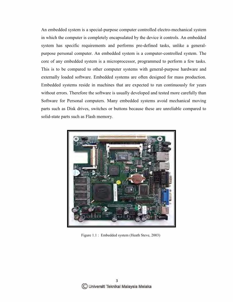
An embedded system is a special-purpose computer controlled electro-mechanical system
in which the computer is completely encapsulated by the device it controls. An embedded
system has specific requirements and performs pre-defined tasks, unlike a general-
purpose personal computer. An embedded system is a computer-controlled system. The
core of any embedded system is a microprocessor, programmed to perform a few tasks.
This is to be compared to other computer systems with general-purpose hardware and
externally loaded software. Embedded systems are often designed for mass production.
Embedded systems reside in machines that are expected to run continuously for years
without errors. Therefore the software is usually developed and tested more carefully than
Software for Personal computers. Many embedded systems avoid mechanical moving
parts such as Disk drives, switches or buttons because these are unreliable compared to
solid-state parts such as Flash memory.
Figure 1.1 : Embedded system (Heath Steve, 2003)
4
1.1 Problem Statement
Nowadays, most of the controller has their weaknesses in performing tasks. Some of the
problem occurred such as less of efficiency in real time application, didn’t get an exactly
position and acceleration during rotation of DC motor, and less torque while in rotating
position. Due to the problem, an embedded system was develop to increase the efficiency
of controller during perform a specific task.
The designer therefore focuses on the controlled object from the beginning to the end of
the development and the implementation issues as MCU, the programming language, the
scheduling policy and the other nonfunctional aspects.
Through this research, this problem will be overcome with the development of an
embedded system and can be implemented in controlling a DC motor with higher
efficiency.
1.2 Objective
This project aims to produce an efficient, precise and good DC motor operating system
during in embedded system that can be achieved by using a PIC16F877A through a
certain programming.
To fulfill the project aim, there are three objectives have been line up and must be
achieved. The main purpose of this embedded system is :
1. To design and develop of an embedded control system.
2. To design a PID controller for an embedded system.
3. To get an exact position during rotation of DC motor.

5
1.3 Scope
This project will mainly focus on development of an embedded system for controlling a
DC motor. The following are the guidelines that listed to ensure that the project is
conducted within its boundary of hardware modification and development, electronics
and programming.
The scope started with hardware modification and development will covered the design
of the circuit for an embedded system. This circuit will create in one software. After the
development of the circuit was done, all components must be arranged in appropriate
position for development of PCB layout. This PCB layout will be used in PCB board for
getting a circuit through an etching process.
Next, electronic components must be considered and should attach on the PCB board.
After development of circuit was done, programming for the PIC16F877A should be
developing using C language. This programming will be downloaded to the PIC16F877A
for circuit operations. Through a programming, a torque, position and acceleration of the
DC motor can be set up. A DC motor consist an encoder that can be used as a feedback
element for controlling a DC motor. Control system element which is PID has been used
for adjusting a gain for the encoder while rotating the DC motor.
For scope of testing the project, the circuit must be confirming on their conductivity. This
test can be done using a conductive test by using a multimeter. This test can check the
conductivity for each component for whole circuit. The circuit must also be tested for its
purpose it builds which is for controlling a torque, position and acceleration of the DC
motor through a program that has been build in programming section. This test can be
done by interfacing the circuit to the computer using USB UART. Several values can be
set up in the programming to look on the performance of the torque, acceleration and
position of the DC motor.
6
1.4 Limitation of Project
All projects have their limitation due to its performances and the way it operates for
specific task. The limitation for this project is :
a) This embedded system will mainly focus for controlling the position of DC
motor.
b) A control system element PID will be attached in this embedded system by
adjusting their gain.
1.5 Project Outline
This project consists of six chapters. Chapter one explains the introduction of the project
including the objective, scope, problem statement and expected outcomes.
Chapter two describes literature review more about previous study on topics that related
to the project. It will cover both, other project research and implementations or
organizations that suitable to relate on embedded system.
Chapter three will cover the methodology of the project. The main topic of this chapter
will describe the method that is used in development an embedded control system and
also the flow chart for the process.
Chapter four illustrates the design and the development. In this chapter, all related
designing the project are mentioned such as hardware designing, electronic circuit
designing and programming using suitable software.
Chapter five will mainly focus on the result and discussion on the project after the project
complete and finally chapter six summarized the project in all field.
7
1.6 Expected Outcomes
Through this preliminary research, the expected outcome is:
a) Achieve the objective for this project which is design an embedded system for
controlling a DC motor.
b) Get an exacted position while rotating a DC motor.
c) Reach a certain value of distances when several values were inserted in a
programming.
1.7 Conclusion
From this chapter, all related information has been introduced in development of an
embedded system for controlling a DC motor. A general purpose computing system is a
combination of generic hardware and general purpose operating system for executing a
variety of applications, where an embedded system is a combination of special purpose
hardware an embedded OS for executing specific applications. This embedded system
was design due to its operation in controlling a DC motor. In designing an embedded
system, all related information has been considered such as the hardware, electric and
electronic part, programming an element of control system. Embedded systems are
designed to serve the purpose of any one or a combination of data collection, storage,
representation data communication, data signal processing (DSP), monitoring, control or
application specific user interface. The boundary of the development of embedded
systems will be discussing more in the next chapter.
10
CHAPTER 2 LITERATURE REVIEW
2.0 Introduction
This chapter will discuss and review available literature on Embedded System using DC
motor. The review begins with the introduction and historical about an embedded system.
This section also will discuss the designing of an embedded system for controlling DC
motor with including the use of PIC in controlling the embedded system such as the
speed, acceleration, position, motion, and torque of DC motor. Then, other related
software and program also will be discussed in this chapter.
2.1 History of An Embedded System
Embedded systems exist even before the IT revolution. In the older days embedded
systems were built around the old vacuum tube and transistor technologies and the
embedded algorithm was developed in low level language. Advances in semiconductor
and nano-technology and IT revolution gave way to the development of miniature
embedded systems. The first recognized modern embedded system is the Apollo
Guidance Computer (AGC) developed by the MIT Instrumentation Laboratory for the
lunar expedition. The Command Module was designed to encircle the moon while the
Lunar Module and its crew were designed to go down to the moon surface and there
safely. [Shibu K V, 2009]
11
Shibu KV (2009) also said that the Lunar Module featured in total 18 engines. There were
16 reaction control thrusters, a descent engine and an ascent engine. The descent engine
was „designed‟ to provide thrust to the lunar module out of the lunar orbit and land it
safely on the moon. MIT‟s original design was based on 4K words of fixed memory
(Read Only Memory) and 256 words of erasable memory (Random Access Memory). By
June 1963, the figures reached 10K of fixed and 1K of erasable memory. The final
configuration was 36K words of fixed memory and 2K words of erasable memory. The
clock frequency of the first microchip proto model used in AGC was 1.024 MHz and it
was derived from a 2.048 MHz crystal clock.
The computing unit of AGC consisted of approximately 11 instruction and 16 bit word
logic. Around 5000 ICs (3-input NOR gates, RTL logic) supplied by Fairchild
Semiconductor were used in this design. The user interface unit of AGC is known as
DSKY (display/keyboard). DSKY looked like a calculator type keypad with an array of
numerals. It was used for inputting the commands to the module numerically. The first
mass-produced embedded system was the guidance computer for the Minuteman-I
missile in 1961. It was the „Autonetics D-17‟ guidance computer, built using discrete
transistor logic and a hard disk for main memory.
Embedded systems encompass a wide range of applications, technologies, and
disciplines, necessitating a broad approach to education. Embedded application include a
small and single-microcontroller applications, control systems, distributed embedded
control, system-on-chip, networking, embedded PCs, critical systems, robotics, computer
peripherals, wireless data systems, signal processing, and command and control.
12
2.2 Definition of An Embedded System
An embedded system is an electronic or electro mechanical system designed to perform a
specific function and is a combination of both hardware and software.[Todd D. Morton,
2001]. Every embedded system is unique, and the hardware as well as the software is
highly specialized to the application domain. Embedded system are becoming an
inevitable part of any product or equipment in all fields including household appliances,
telecommunications, medical equipment, industrial control and consumer product.
Additional cross-cutting skills that are important to embedded system designers include
security, dependability, energy computing, software or systems engineering, real-time
computing, and human computer interaction.
According to the Shibu K V (2009), the first integrated circuit was produced in
September 1958 but computers using them didn‟t begin to appear until 1963. Some of
their early uses were in embedded systems, notably used by NASA for the Apollo
Guidance Computer and by the US military in the Minuteman-II intercontinental ballistic
missile. Embedded systems are designed for a specific application from the characteristic
of the embedded systems. The software of the embedded systems is unalterable by the
end user.
Embedded software systems typically run on dedicated hardware, and are systems in
which a primary objective is typically to control external devices. Embedded software
systems are found in a number of applications, such as in aircraft flight control, reactor
protection systems, medical electronic devices, washing machines, and mobile phones. A
lack of direct user involvement or supervision requires highly reliable and efficient
software, which must typically work in real-time, as embedded systems respond to and
control real-world events.
13
2.3 Characteristic and Reliability of Embedded Systems. In do some operation, embedded system has their own characteristic. This characteristic
shows the ability of the embedded system while performing an operation. Embedded
systems are designed to do a specific task, unlike general-purpose computers. Some
embedded systems have real-time "performance constraints" that must be meet, for
reasons such as safety and usability without constraints the systems are simplified at low
price. [Greg Osborn, 2010].
Embedded systems are not always standalone devices. Many embedded systems consist
of small, computerized parts within a larger device that serves a more general purpose.
Similarly, an embedded system in a car provides a specific function as a subsystem of the
car itself.
The program instructions written for embedded systems are referred to as software, and
are stored in read-only memory or flash memory chips. They run with limited computer
hardware resources: little memory, small or non-existent keyboard or screen.
Greg Osborn (2010) also said that embedded systems often in machines that are expected
to run continuously for years without errors and in some cases recover by themselves if
an error occurs. Therefore the software is usually developed and tested more carefully
than that for personal computers, and unreliable mechanical moving parts such as disk
drives, switches or buttons are avoided.
14
2.4 Purpose of Embedded Systems. As mentioned in the previous section, embedded systems are used in various domains like
consumer electronics, home automation, telecommunications, automotive industry,
healthcare, control and instrumentation, retail and banking applications. Within the
domain itself, according to the application usage context, they may have different
functionalities. Each embedded system is designed to serve the purpose of any task.
2.4.1 Data Collection and Storage Representation
Embedded systems are designed for the purpose of data collection performed from the
real world. Data collection is usually done for storage, analysis, manipulation and
transmission. The term "data" refers all kinds of information, text, voice, image, video,
electrical signals and any other measurable quantities. Data can be either analog
(continuous) or digital (discrete).
Embedded systems with analog data capturing techniques collect data directly in the form
of analog signals whereas embedded systems with digital data collection mechanism
converts the analog signal to corresponding digital signal using analog to digital (A/D)
converters and then collects the binary equivalent of the analog data. If the data is digital,
it can be directly captured without any additional interface by digital embedded systems.
[Shibu K V, 2009]
The collected data may be stored directly in the system or may be transmitted to some
other systems or it may be processed by the system or it may be deleted instantly after
giving a meaningful representation. These actions are purely dependent on the purpose
for which the embedded system is designed. Embedded systems designed for pure
measurement applications without storage, used in control and instrumentation domain
collects data and gives a meaningful representation of the collected data.
15
2.4.2 Data Communication.
Todd D. Morton, (2001) said that an embedded data communication systems are
developed in applications ranging from complex satellite communication systems to
simple home networking systems As mentioned earlier in this chapter, the data collected
by an embedded terminal may require transferring of the same to some other system
located remotely. The transmission is achieved either by a wire line medium or by a
wireless medium Wire-line medium was the most common choice in all olden days
embedded systems. As technology is changing, wireless medium is becoming the DC-
facto standard for data communication in embedded systems. A wireless medium offers
cheaper connectivity solutions and make the communication link free from the hassle of
wire bundles. Data can either be transmitted by analog means or by digital means.
Modern industry trends are settling towards digital communication.
2.4.3 Data Signal Processing (DSP)
As mentioned earlier, the data (voice, image, video, electrical signals and other
measurable quantities) collected by embedded systems may be used for various kinds of
data processing. Embedded systems with signal processing functionalities are employed
in applications demanding signal processing like speech coding, synthesis, audio video
codec, transmission applications and others. A digital hearing aid is a typical example of
an embedded system employing data processing. Digital hearing aid improves the hearing
capacity of hearing impaired persons. [Bennett, Stuart ,1993].
16
2.5 Design and Development of An Embedded System.
In designing an embedded system, several aspect must be considered such as the purpose
for it designing, the controller, how to interface that system and programming. Normally,
the purpose for building an embedded system is to control some element such as motor,
temperature, movement and to locate a memory. With the application of an embedded
system, several task and purpose can be completed.
In this project, some information are needed in related journal to identify an element in
designing an embedded control system. All inform that are gathered and related are
discussed here for further perusal in achieving the objective of this project.
An Embedded system has been built to solve only a few very specific problems. Very
often, such systems must give an answer in a specified time. This is called real-time
computing. These computers are usually embedded and offer different devices. In
contrast, a general-purpose computer can do many different tasks depending on
programming. Embedded systems control many of the common devices in use today.
[Shibu K V ,2009].
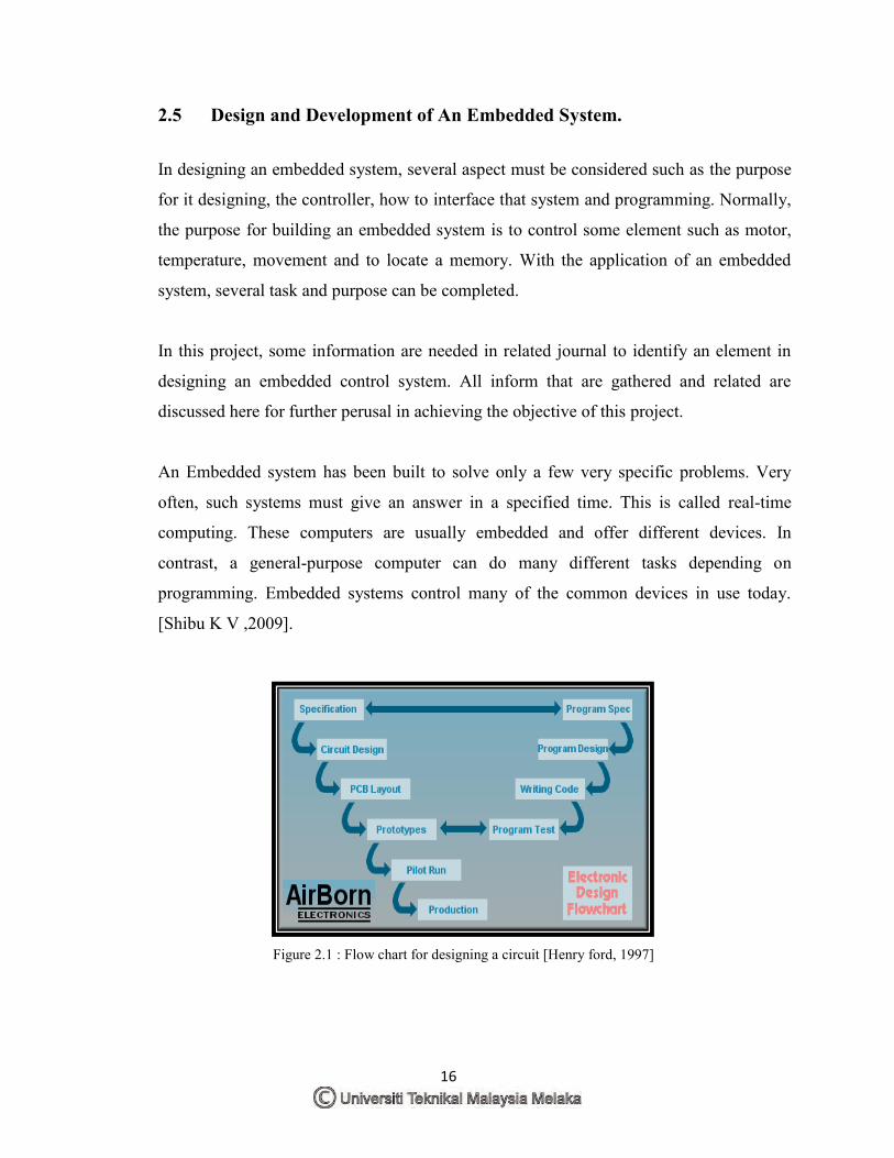
Figure 2.1 : Flow chart for designing a circuit [Henry ford, 1997]
17
There are several techniques that must be taken in designing an embedded system. This
technique played an important role and give a bad impact to the designing an embedded
systems. The techniques in designing an embedded system usually started with build a
schematic diagram, identify the controller, how to interface the controller and developed
a suitable programming to give an instruction in handling the embedded system. Even
though, this technique is related in designing a system that have a controller within it
boundaries.
2.5.1 Schematic Design. A circuit diagram is a strict document, and cannot be "mostly correct". A circuit diagram
must reflect the actual construction of the printed circuit board which is made from it,
exactly. A good circuit diagram will include extra information required to understand the
circuit operation, have descriptive net and connector labels, and include all of the parts on
the printed circuit board. [Vladimir Gurevich, 2008]
Naveed Sherwani , (2001) said that the design process involves moving from the
specification at the start, to a plan that contains all the information needed to be
physically constructed at the end, this normally happens by passing through a number of
stages, although in very simple circuit it may be done in a single step. The process
normally begins with the conversion of the specification into a block diagram of the
various functions that the circuit must perform, at this stage the contents of each block are
not considered, only what each block must do, this is sometimes referred to a design. This
approach allows the possibly very complicated task to be broken into smaller tasks.
Dr Steve C. Hsiung, (2007) said in his journal that each block must considered in more
detail, but with a lot more focus on the details of the electrical functions to be provided.
At this or later stages it is common to require a large amount of research or mathematical
modeling into what is and is not feasible to achieve.
18
The results of this research may be fed back into earlier stages of the design process, for
example if it turns out one of the blocks cannot be designed within the parameters set for
it, it may be necessary to alter other blocks instead. At this point it is also common to start
considering both how to demonstrate that the design does meet the specifications, and
how it is to be tested.
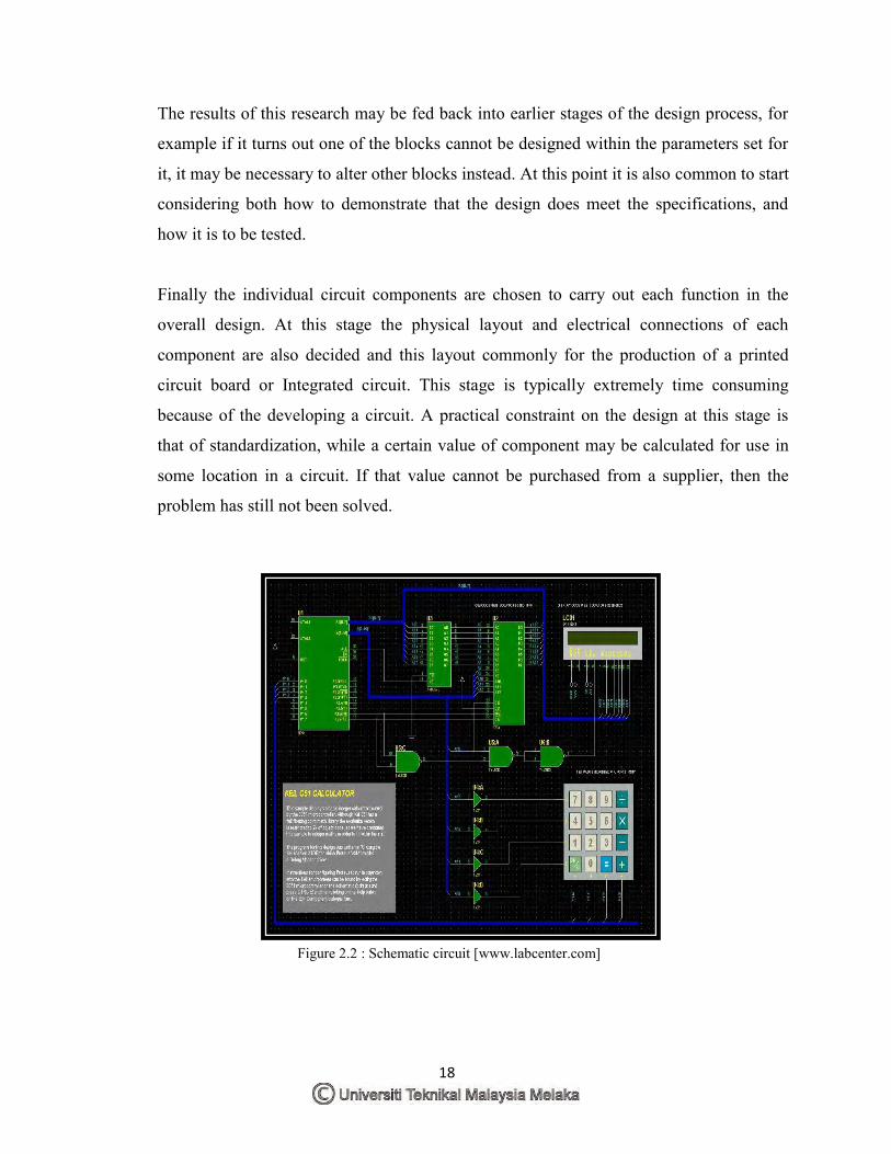
Finally the individual circuit components are chosen to carry out each function in the
overall design. At this stage the physical layout and electrical connections of each
component are also decided and this layout commonly for the production of a printed
circuit board or Integrated circuit. This stage is typically extremely time consuming
because of the developing a circuit. A practical constraint on the design at this stage is
that of standardization, while a certain value of component may be calculated for use in
some location in a circuit. If that value cannot be purchased from a supplier, then the
problem has still not been solved.
Figure 2.2 : Schematic circuit [www.labcenter.com]
19
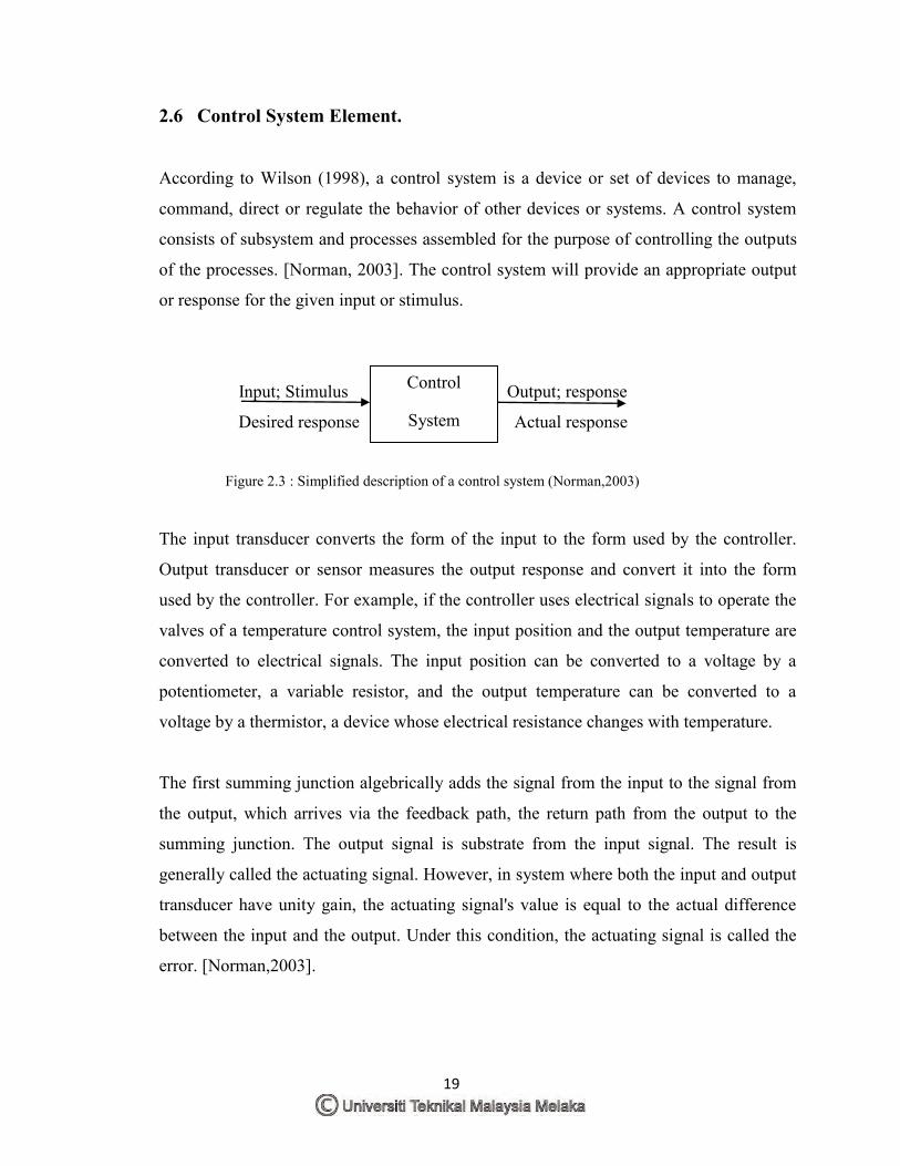
2.6 Control System Element.
According to Wilson (1998), a control system is a device or set of devices to manage,
command, direct or regulate the behavior of other devices or systems. A control system
consists of subsystem and processes assembled for the purpose of controlling the outputs
of the processes. [Norman, 2003]. The control system will provide an appropriate output
or response for the given input or stimulus.
Input; Stimulus Output; response
Desired response Actual response
Figure 2.3 : Simplified description of a control system (Norman,2003)
The input transducer converts the form of the input to the form used by the controller.
Output transducer or sensor measures the output response and convert it into the form
used by the controller. For example, if the controller uses electrical signals to operate the
valves of a temperature control system, the input position and the output temperature are
converted to electrical signals. The input position can be converted to a voltage by a
potentiometer, a variable resistor, and the output temperature can be converted to a
voltage by a thermistor, a device whose electrical resistance changes with temperature.
The first summing junction algebrically adds the signal from the input to the signal from
the output, which arrives via the feedback path, the return path from the output to the
summing junction. The output signal is substrate from the input signal. The result is
generally called the actuating signal. However, in system where both the input and output
transducer have unity gain, the actuating signal's value is equal to the actual difference
between the input and the output. Under this condition, the actuating signal is called the
error. [Norman,2003].
Control
System
20
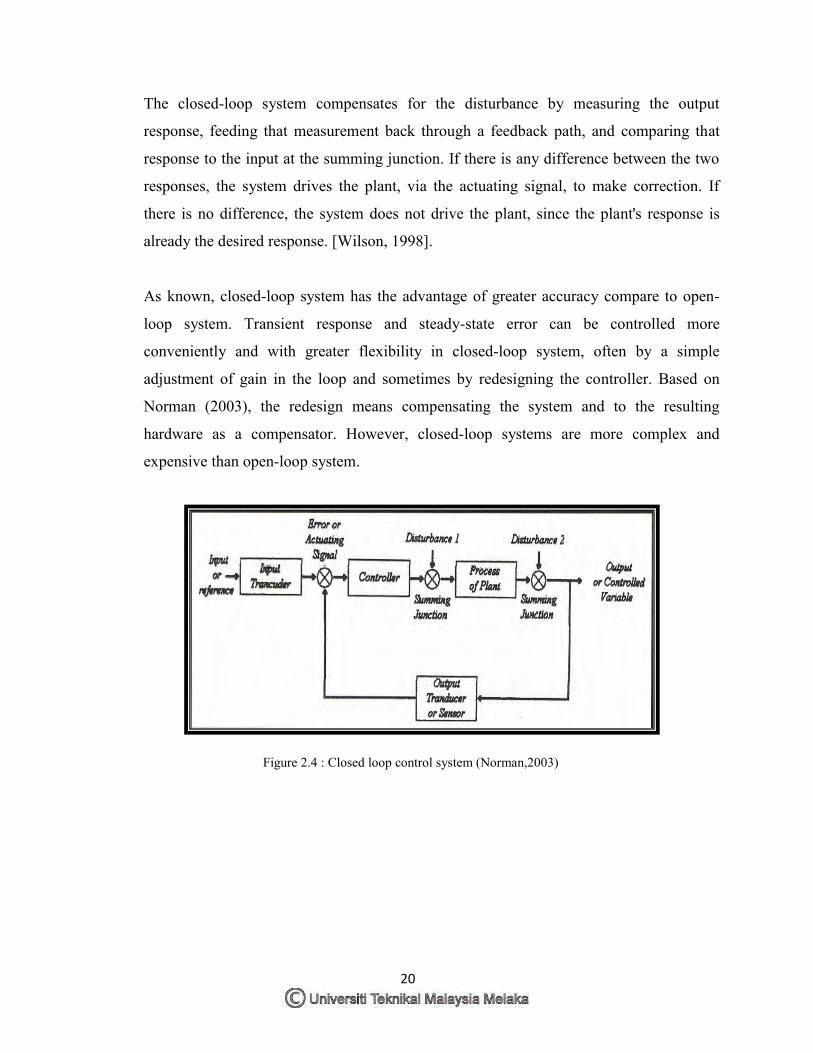
The closed-loop system compensates for the disturbance by measuring the output
response, feeding that measurement back through a feedback path, and comparing that
response to the input at the summing junction. If there is any difference between the two
responses, the system drives the plant, via the actuating signal, to make correction. If
there is no difference, the system does not drive the plant, since the plant's response is
already the desired response. [Wilson, 1998].
As known, closed-loop system has the advantage of greater accuracy compare to open-
loop system. Transient response and steady-state error can be controlled more
conveniently and with greater flexibility in closed-loop system, often by a simple
adjustment of gain in the loop and sometimes by redesigning the controller. Based on
Norman (2003), the redesign means compensating the system and to the resulting
hardware as a compensator. However, closed-loop systems are more complex and
expensive than open-loop system.
Figure 2.4 : Closed loop control system (Norman,2003)
21
2.6.1 PID Definition and Element.
A PID controller has been used in order to regulate particular closed loop systems. A
proportional–integral–derivative controller (PID controller) is a generic control loop
feedback mechanism (controller) widely used in industrial control systems. A PID is the
most commonly used feedback controller. A PID controller calculates an "error" value as
the difference between a measured process variable and a desired set point. The controller
attempts to minimize the error by adjusting the process control inputs. In the absence of
knowledge of the underlying process, a PID controller is the best controller. [Bennett,
Stuart 1993].
The PID controller calculation (algorithm) involves three separate parameters, and is
accordingly sometimes called three-term control: the proportional, the integral and
derivative values, denoted P, I, and D. The proportional value determines the reaction to
the current error, the integral value determines the reaction based on the sum of recent
errors, and the derivative value determines the reaction based on the rate at which the
error has been changing. [Ang, K.H, 2005]
Antonio Visioli (2006), said that a controller can be used to control any measurable
variable which can be affected by manipulating some other process variable. For
example, it can be used to control temperature, pressure, flow rate, chemical cornposition,
speed, or other variables. The PID control scheme is named after its three correcting
terms, whose sum constitutes the output.
1. Proportional - To handle the immediate error, the error is multiplied by a constant
Kp. Note that when the error is zero, a proportional controller's output is zero.
However, the proportional controller will not reach the set point if a non-zero
output is required to maintain the set point. For example, consider a controller that
is attempting to maintain the temperature in a room by controlling a heating
element with varying heat loss due to a changing outside temperature.
22
The output to the heating element that will maintain the set point perfectly where
the outside temperature 20 degrees less than the room set point will cause the
room to be too warm if the outside temperature is warmer (and the room will be
too cold if the outside temperature is colder). This is called a "steady state error”.
To fix this an Integral component must be added to the controller.
2. Integral - To learn from the past, the error is integrated and multiplied by a
constant Kt. The integral term allows a controller to eliminate a steady state error
if the process requires a non-zero input to produce the desired set point. An
integral controller will react to the error by accumulating a value that is added to
the output value. While this will force the controller to approach the setpoint
quicker than a proportional controller alone and eliminate steady state error, it also
guarantees that the process will overshoot the set point since the integral value
will continue to be added to the output value.
3. Derivative - To anticipate the future, the first derivative of the error is multiplied
by a constant Kd. This can be used to reduce the magnitude of the overshoot,
produced by the integral component, but the controller will be a bit slower to
reach the set point initially.
The terms of controller as: P -Proportional, I - Integral, D - Derivative. These terms
describe three basic mathematical functions applied to the error signal , Verror =Vset -
Vsensor. This error represents the difference between where you want to go (Vset), and
where you're actually at (Vsensor). The controller performs the PID mathematic functions
and the error and applies the their sum to a process. Tuning a system means adjusting
three multipliers Kp, Ki and Kd adding in various amounts of these functions to get the
system that suitable for process requirement.
23
2.6.2 PID Application
Most controller today has their own element for accomplish specific task. For getting a
higher transient response in several task, a control system element is likely to be used. On
top of that in reaching a higher transient response, a PID controller has been used. Below
is several related task that used a PID controller in their project.
Suppose a water tank is used to supply water for use in several parts of a plant, and it is
necessary to keep the water level constant. A sensor would measure the height of water in
the tank, producing the measurement, and continuously feed this data to the controller.
The controller would have a set point of (for example) half full. The controller would
have its output (the action) connected to a valve controlling the water feed. The controller
would use the measurement of the level to calculate how to manipulate the control valve
to maintain the desired level.[ M H Moradi, 2003]
Abu Bakar (2007) said in his experiments for controlling the heating of a tank. For simple
control, there are two temperature limit sensors (one low and one high) and then switch
the heater ON when the low temperature limit sensor turns on and then turn the heater off
when the temperature rises to the high temperature limit sensor. This is similar to most
home air conditioning and heating thermostats.
In contrast, the PID controller would receive as input the actual temperature and control a
valve that regulates the flow of gas to the heater. The PID controller automatically finds
the correct (constant) flow of gas to the heater that keeps the temperature steady at the set
point. Instead of the temperature bouncing back and forth between two points, the
temperature is held steady. If the set point is lowered, then the PID controller
automatically reduces the amount of gas flowing to the heater. If the set point is raised,
then the PID controller automatically increases the amount of gas following to the heater.
Likewise the PID controller would automatically compensate for hot, sunny days (when it
is hotter outside the heater) and for cold, cloudy days.[Michail Petrov, 2002].
24
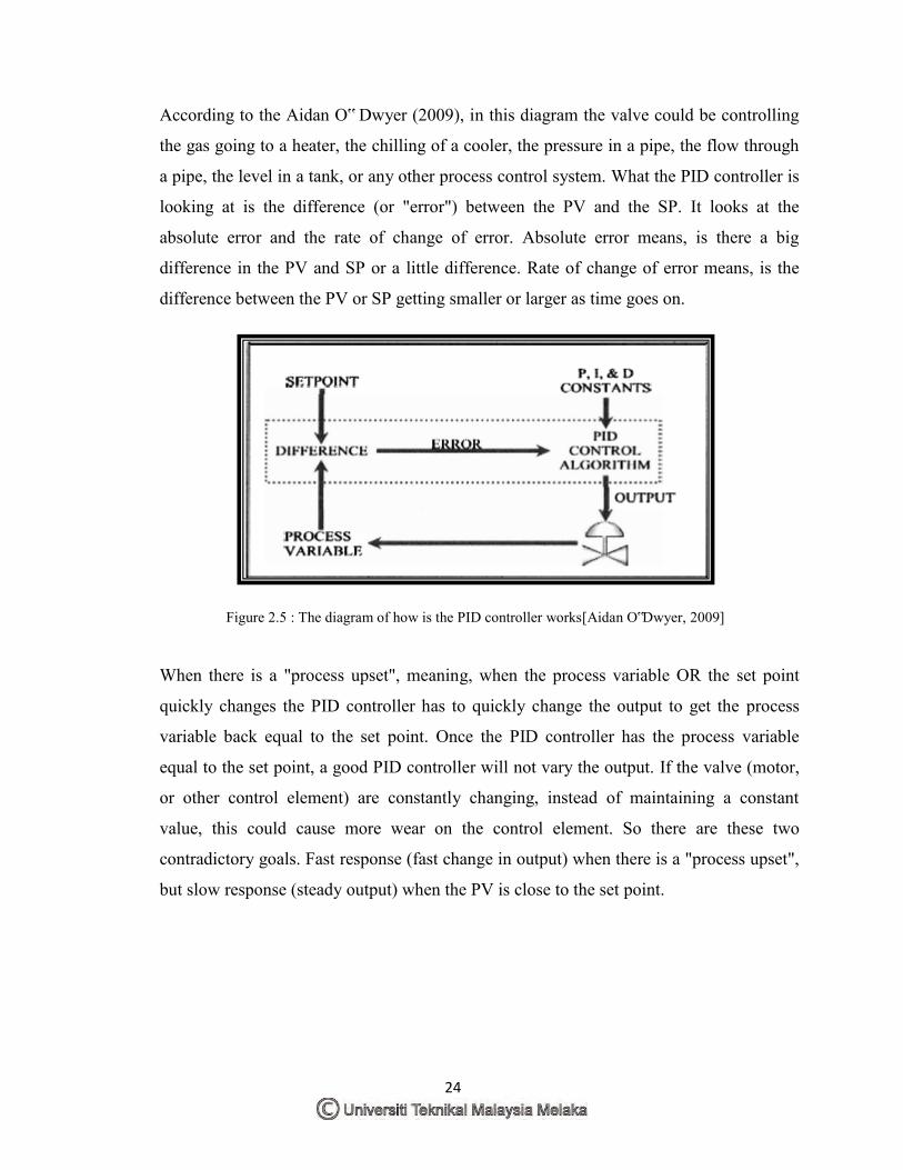
According to the Aidan O‟ Dwyer (2009), in this diagram the valve could be controlling
the gas going to a heater, the chilling of a cooler, the pressure in a pipe, the flow through
a pipe, the level in a tank, or any other process control system. What the PID controller is
looking at is the difference (or "error") between the PV and the SP. It looks at the
absolute error and the rate of change of error. Absolute error means, is there a big
difference in the PV and SP or a little difference. Rate of change of error means, is the
difference between the PV or SP getting smaller or larger as time goes on.
Figure 2.5 : The diagram of how is the PID controller works[Aidan O‟Dwyer, 2009]
When there is a "process upset", meaning, when the process variable OR the set point
quickly changes the PID controller has to quickly change the output to get the process
variable back equal to the set point. Once the PID controller has the process variable
equal to the set point, a good PID controller will not vary the output. If the valve (motor,
or other control element) are constantly changing, instead of maintaining a constant
value, this could cause more wear on the control element. So there are these two
contradictory goals. Fast response (fast change in output) when there is a "process upset",
but slow response (steady output) when the PV is close to the set point.
25
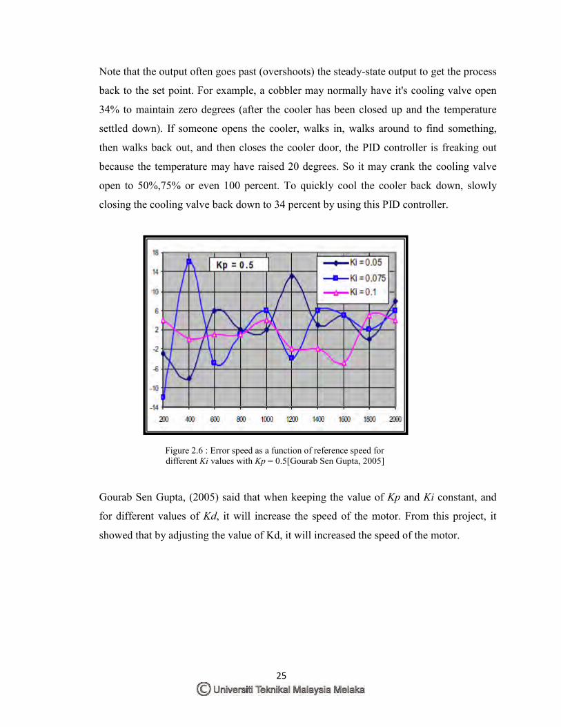
Note that the output often goes past (overshoots) the steady-state output to get the process
back to the set point. For example, a cobbler may normally have it's cooling valve open
34% to maintain zero degrees (after the cooler has been closed up and the temperature
settled down). If someone opens the cooler, walks in, walks around to find something,
then walks back out, and then closes the cooler door, the PID controller is freaking out
because the temperature may have raised 20 degrees. So it may crank the cooling valve
open to 50%,75% or even 100 percent. To quickly cool the cooler back down, slowly
closing the cooling valve back down to 34 percent by using this PID controller.
Figure 2.6 : Error speed as a function of reference speed for different Ki values with Kp = 0.5[Gourab Sen Gupta, 2005]
Gourab Sen Gupta, (2005) said that when keeping the value of Kp and Ki constant, and
for different values of Kd, it will increase the speed of the motor. From this project, it
showed that by adjusting the value of Kd, it will increased the speed of the motor.
26
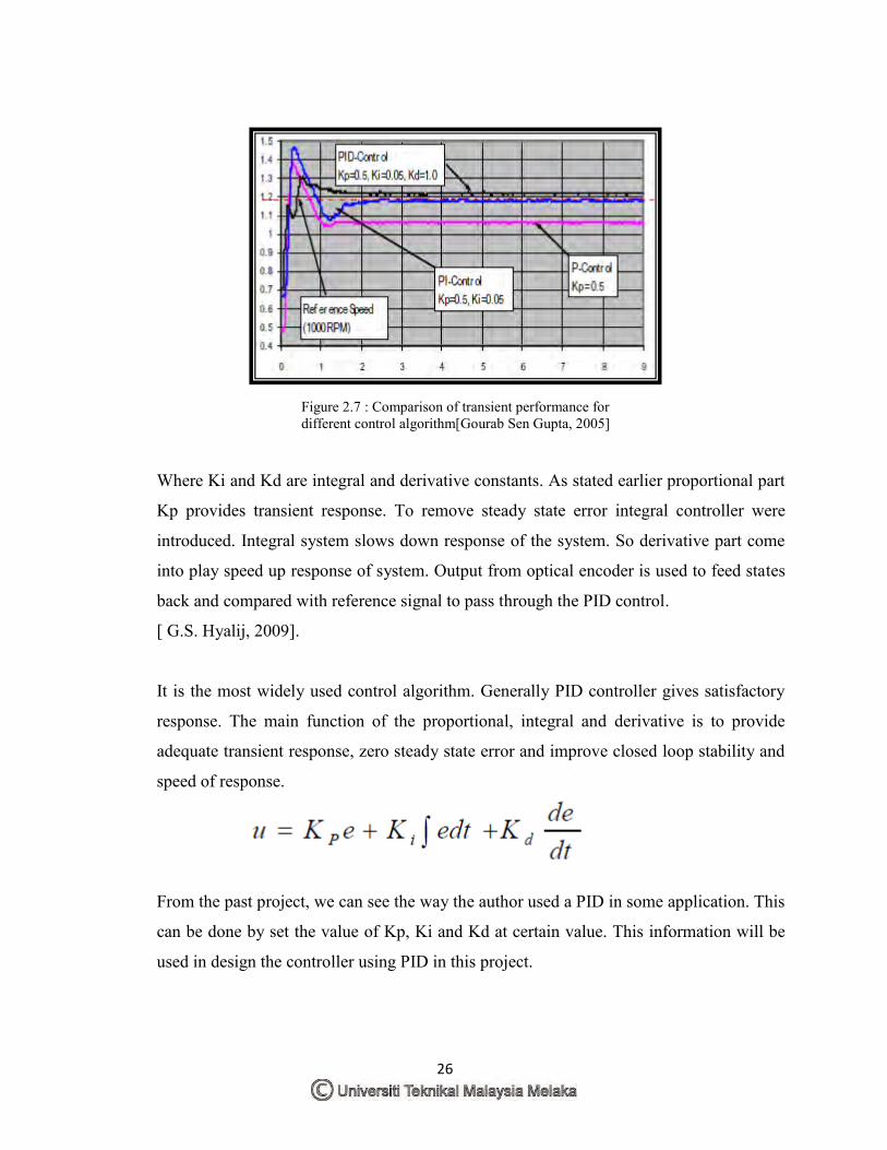
Figure 2.7 : Comparison of transient performance for different control algorithm[Gourab Sen Gupta, 2005]
Where Ki and Kd are integral and derivative constants. As stated earlier proportional part
Kp provides transient response. To remove steady state error integral controller were
introduced. Integral system slows down response of the system. So derivative part come
into play speed up response of system. Output from optical encoder is used to feed states
back and compared with reference signal to pass through the PID control.
[ G.S. Hyalij, 2009].
It is the most widely used control algorithm. Generally PID controller gives satisfactory
response. The main function of the proportional, integral and derivative is to provide
adequate transient response, zero steady state error and improve closed loop stability and
speed of response.
From the past project, we can see the way the author used a PID in some application. This
can be done by set the value of Kp, Ki and Kd at certain value. This information will be
used in design the controller using PID in this project.
27
2.6.3 Proportional-Integral (PI) Speed Controller Although the relevant literatures as discussed have more advanced controllers method,
the proportional-integral, PI control scheme is commonly regarded as one of the strongest
contender to succeed in industrial applications. In fact, this scheme is most popular in
implementation of driving the SRM (Switch Reluctance Motor) due to its simplest
controller strategy and it provides good performance. PI controllers are comprehensively
applied in various drives, where the speed control is desired. The reasons for this include
lower cost, good speed response, simplicity and easy of implementation, and ability to
achieve steady state error. Therefore, in this thesis, a speed controller based on the PI
control strategy is designed as a tool to implement a variable speed drive mechanism
which is essentially needed in speed performance analysis.
According to the Asri bin Din, (2008), the 60 kW SRM model is tested, which is
considered as in a medium power capacity. The rated external load is about 96 Nm and
the maximum speed can reached up to 6000 rpm. In practice, an oversize of the machine
and rated operating level are taken into consideration. Therefore, the analysis in this
thesis is analyzed at rated speed of 3600 rpm and below. In addition, the maximum load
to be tested is at its rated external load torque, which is 96 Nm.
In static and dynamic load simulation, the external load torque is divided into four types
of load which are according to the percentage of several rated external load torque. They
are divided into 25% (24 Nm), 50% (48 Nm), 75% (86 Nm) and 100% (96Nm). For static
external load torque testing, the fixed load is applied to the rotor shaft starting from the
motor at a stand still condition. Then, the applied load is still maintained throughout the
motor operation, up to the steady state level. The importance of this type of simulation is
easier to be understood if the particular condition relates to the application of the motor
presented.
28
Sharma (1996), in a study, briefly discussed the choosing of the optimum combination of
switching angels. The switching states are based on a set of fuzzy variables, which are
characterized by expressions and it is used to generate torque reference for optimum
performance. As an important element that potentially affects the speed response, the
effect under variations of switching angles is proposed to be analyzed in this thesis. The
evaluation is done in order to compare the three types of the switch-on and the switch-off
combination. The comparisons were observed in terms of the three phase-current
switching, the average of torque production shape and the speed response.
2.7 Controller in Embedded System
Embedded systems with control functionalities impose control over some variables
according to the changes in input variables. For an example, a one system with control
functionality contains both sensors and actuators. Sensors are connected to the input port
for capturing the changes in environmental variable or measuring variable. The actuators
connected to the output port are controlled to the changes in input variable to put an
impact on the controlling variable to bring the controlled variable to the specified range.
Y. S. E. Ali, (2003) said that the use of power electronics for the control of electric
machines offers not only better performance caused by precise control and fast response,
but also maintenance, and ease of implementation. In power electronic there have been
great advances in controller based control systems due to the flexibility and versatility.
This is because the entire control algorithm is implemented in the software.
For this project, a microcontroller has been used for controlling a DC motor. With the
variety of the microcontroller, it can be programmed due to the specific task that is need
by the user.
29
2.7.1 Microcontroller Definition.
Microcontrollers are found in almost all "smart" electronic devices. From microwaves to
automotive braking systems, they are around us doing jobs that make our lives more
convenient and safer. Microcontrollers are essentially small computers. Unlike your
desktop computer, microcontrollers interact with other machines rather than humans. A
microcontroller might be used to measure the temperature of your toast at breakfast and
when the temperature reaches a predetermined measure, the toaster could be turned off. A
microcontroller could also be used to count the number of customers entering the ball
park through a turnstile thereby keeping track of ticket sales. The uses for these small
versatile devices are diverse. Perhaps you can imagine a microcontroller application that
will improve a product or decrease the time required to complete a process.
A microcontroller is a small computer on a single integrated circuit containing a
processor core, memory, and programmable input/output peripherals. Microcontrollers
provide low-cost computing and automated decision-making capabilities to numerous
machines, products, and processes. Commonly, microcontrollers are embedded directly
into automated machines/products and neither require nor permit user interaction.[I. Scott
Mackenzie, 2007]
According to the Giovino Bill (2003), a microcontroller can be considered a self-
contained system with a processor, memory and peripherals and can be used as an
embedded system. The majority of microcontrollers in use today are embedded in other
machinery, such as automobiles, telephones, appliances, and peripherals for computer
systems.
30
2.7.2 Microcontroller Application.
Some microcontrollers may use four-bit words and operate at clock rate frequencies as
low as 4 kHz, for low power consumption (milliwatts or microwatts). They will generally
have the ability to retain functionality while waiting for an event such as a button press or
other interrupt; power consumption while sleeping may be just nano watts, making many
of them well suited for long lasting battery applications. Other microcontrollers may
serve performance-critical roles, where they may need to act more like a digital signal
processor (DSP), with higher clock speeds and power consumption.[Shibu KV,2009]
Dr. Steve C. Hsiung, (2007) said in his article that the selected design is to have multiple
slave processors that everyone is in the same format. This design is to modularize the
processor environment that has a single master which takes the control commands from a
user and passes the necessary control functions to an appropriate slave to perform the
operations. With this design concept, there will be virtually no limit on the number of
slaves in the system.
From the Dr Steve C. Hsiung project, we can see that the processor will control
commands from a user and passes that command to the controller. This will help in make
the communication become an easier.
The limitations in the previous design on a single CPU approach are automatically
resolved. Certainly, this approach requires a well planned software protocol design, and
the hardware requirement becomes a fixed module that is less complex (Philips, 1997),
and thus the following section on hardware, software designs, and their implementation
as a proof of concept of multiple processors in multiple DC motors control applications in
an applied research on the use of multiple PIC 16F84As in a system design is convinced,
low cost, and efficient.
31
The 68HClIE9 microcontroller implements the control algorithm by conditioning the
speed and current signals and performs the speed regulation according to speed reference.
The software includes a routine to read the motor current and sends emergency shutdown
signal to protect the DC motor from over current, also this signal can be activated
manually by inserting a designated character by the keypad, which causes a software
interrupt and executes the emergency shutdown routine.[ Y. S. E. Ali, 2003].
Nicolai and Castagnet (1993), have shown in their paper how a microcontroller can be
used for speed control. The operation of the system can be summarized as the drive form
a rectified voltage, it consists of chopper driven by a PWM signal generated from a
microcontroller unit (MCU). The motor voltage control is achieved by measuring the
rectified mains voltage with the analog to digital converter present on the microcontroller
and adjusting the PWM signal duty cycle accordingly.
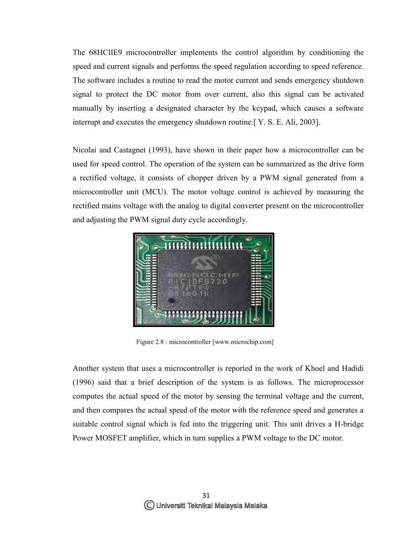
Figure 2.8 : microcontroller [www.microchip.com]
Another system that uses a microcontroller is reported in the work of Khoel and Hadidi
(1996) said that a brief description of the system is as follows. The microprocessor
computes the actual speed of the motor by sensing the terminal voltage and the current,
and then compares the actual speed of the motor with the reference speed and generates a
suitable control signal which is fed into the triggering unit. This unit drives a H-bridge
Power MOSFET amplifier, which in turn supplies a PWM voltage to the DC motor.
32
2.8 Method for Controlling DC Motor
Electric motors are frequently used as the final control element in positional or speed
control system. Motors can be classified into two main categories which is DC motor and
ac motor. Most motors used in modern control systems is a DC motor. In the
conventional DC motor, coils of wire are mounted in the slots on a cylinder of magnetic
material called the armature. The armature is mounted on bearings and is free to rotate. It
is mounted in the magnetic field produced by field poles. The direction of rotation of the
DC motor can be reversed by reversing either the armature current or the field current.
[W Bolton, 2003]
The basic principles involved in the action of a motor are :
1. A force is exerted on a conductor in a magnetic field when a current passes
through it. For a conductor of length, it is carrying a current I in a magnetic field
of flux density at right angles to the conductor.
2. When a conductor moves in a magnetic field then an e.m.f is induced across it.
The induced e.m.f is equal to the rate at which the magnetic flux swept through by
the conductor changes. The minus sign is because the e.m.f is in such a direction
as to oppose the change producing it. The direction of the induced e.m.f is in such
a direction as to produce a current which sets up magnetic fields which tend to
neutralize the change in magnetic flux linked by the coil.
DC brush motors are increasingly required for a broad range of applications including
robotics, portable electronics, sporting equipment, appliances, medical devices,
automotive applications, power tools and many others. The motor itself is a preferred
alternative because it is simple, reliable and low cost. Equally important, advanced, fully-
integrated "H-bridge" driver ICs are available to control the motor's direction, speed and
braking. H-bridge drivers has been used and discuss the advancement of the technology
from discrete solutions to highly-integrated ICs. It will compare linear motor speed
33
control with more advanced, higher-efficiency pulse-width modulation (PWM)
techniques.[ Tony D. Givargis, 2001]
A parameter based representation of DC motor driving an inertial load, shows the angular
rate of the load, ώ(t), as the output and applied voltage, V(t), as the input. The magnetic
field is assumed to be constant. The nomenclature used are R is the resistance of the
circuit, L is the self-inductance of the armature, I is the current through the coil, J is the
moment of inertia of the load, Km is the armature constant, Kb is the back-emf constant,
Kf (ώ) is a linear approximation for viscous friction, τ is the torque seen at the shaft of the
motor, the differential equations that describe the behavior of this electromechanical
system. [Tanmay Pal, 2009].
DC motor design generates an oscillating current in a wound rotor, or armature, with a
split ring commutator, and either a wound or permanent magnet stator. A rotor consists of
one or more coils of wire wound around a core on a shaft. An electrical power source is
connected to the rotor coil through the commutator and its brushes, causing current to
flow in it, producing electromagnetism. The commutator causes the current in the coils to
be switched as the rotor turns, keeping the magnetic poles of the rotor from ever fully
aligning with the magnetic poles of the stator field, so that the rotor never stops but rather
keeps rotating indefinitely.[ John Catsoulis, O'Reilly, May 2005]
The universal motor is a low-cost solution with limited performance. It is used widely in
the consumer-products industry, especially for power tools and home appliances such as
washers, mixers, vacuum cleaners, etc. This type of motor is called a “universal” motor
because it can run on either AC or DC power. [Huangsheng Xu , 2007]
34
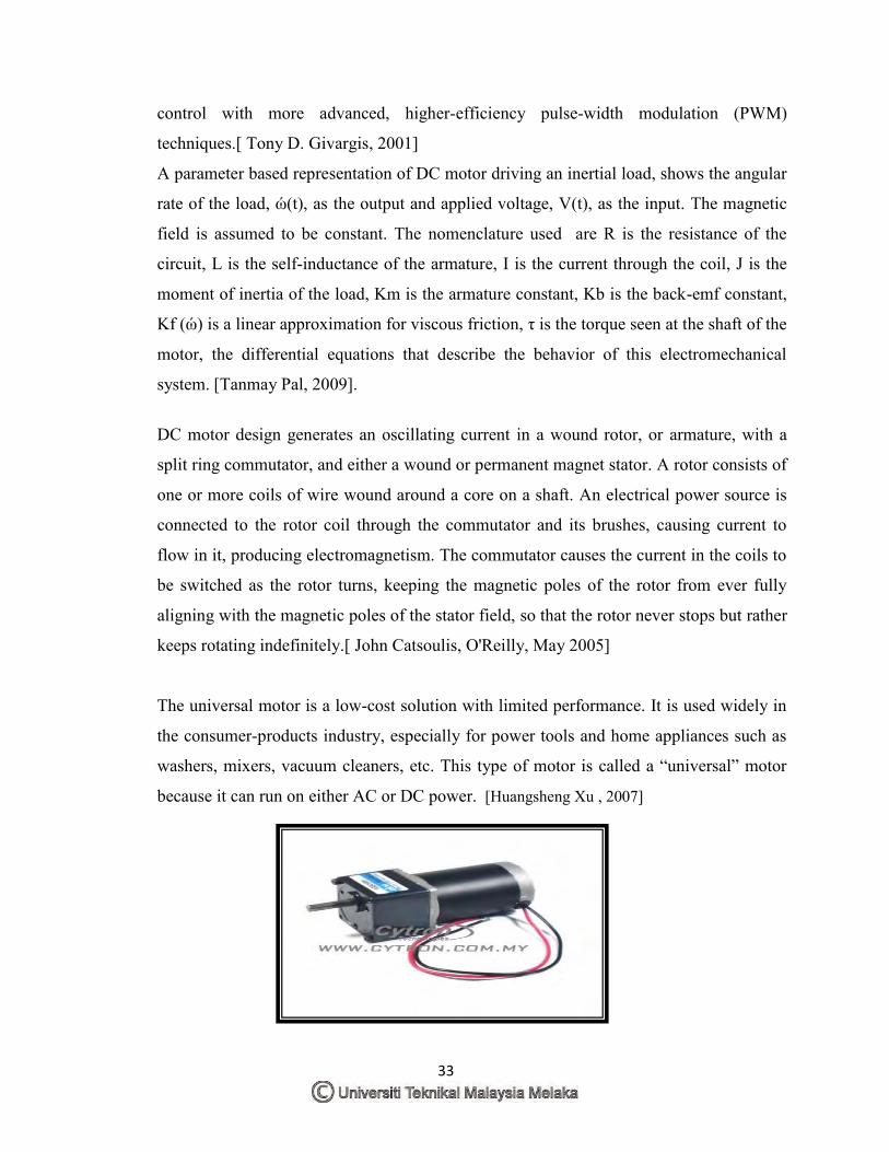
Figure 2.9 : Brush DC Motor (www.cytron.com.my)
Alexander G. Mikerov , 2009 said that the torque motors are assumed to be incorporated in
any controlled plant or machine without any gear or other mechanical transmission. It
delete backlashes, resiliencies, kinematics errors and other mechanical problems which
reduce a drive mechanical resonance frequencies, aggravate the problem of stability and
as a result reduce the control drive accuracy and bandwidth.
2.8.1 Controlling Using Pulse Width Modulator
According to the Michael Barr, (2001), pulse width modulation (PWM) is a powerful
technique for controlling analog circuits with a processor's digital outputs. PWM is
employed in a wide variety of applications, ranging from measurement and
communications to power control and conversion. A constant PWM signal varying from
50% to 90% is applied from the microcontroller, amplified by Interfacing circuit and
driving the motor to speeds 30 Hz to 100 Hz. [Tanmay Pal, 2009]
The frequency of the PWM signal that drives the motor should be high enough so that a
minimal amount of current ripple is induced in the windings of the DC motor. The
amount of current ripple can be derived from the PWM frequency, motor winding
resistance, and motor inductance. More importantly, the PWM frequency is chosen to be
just outside the audible frequency range. Depending on how much hearing loss you've
suffered, a PWM frequency in the 15 kHz - 20 kHz range will be fine. There's no need to
set the PWM frequency any higher; this will only increase the switching losses in the
motor driver IC. [Stephen Bowling, 2000]
When designing a PWM unit using the MCU two factors should be considered PWM
duty cycle, and PWM frequency. The PWM frequency, in this work, is kept constant
factor. It directly affects the DC motor stability and sensibility to changes in its input
voltage. However the frequency can be changed manually within ripper and lower limits
to make the system flexible and able 10 operate motors with different ratings and speeds.
35
According to the Y. S. E. Ali, (2003), the conventional digital proportion MCU technique
and the pulse width modulation (PWM) technique are adopted in DC motor control
system. An optical encoder was used to measure the speed of the motor. The output of the
encoder is a stream of pulses with variable' frequency according to the speed of the
motor.
In a nutshell, PWM is a way of digitally encoding analog signal levels. Through the use
of high-resolution counters, the duty cycle of a square wave is modulated to encode a
specific analog signal level. The PWM signal is still digital because, at any given instant
of time, the full DC supply is either fully on or fully off. The voltage or current source is
supplied to the analog load by means of a repeating series of on and off pulses. The on-
time is the time during which the DC supply is applied to the load, and the off-time is the
period during which that supplies is switched off. Given a sufficient bandwidth, any
analog value can be encoded with PWM. [Micheal Barr, 2001]
To start PWM operation, the suggests software should:
Set the period in the on-chip timer/counter that provides the modulating square wave
Set the on-time in the PWM control register
Set the direction of the PWM output, which is one of the general-purpose I/O pins
Start the timer and enable the PWM controller
S3C2410 PWM Timers have a double buffering function, enabling the reload value
changed for the next timer operation without stopping the current timer operation. So,
although the new timer value is set, a current timer operation is completed successfully.
[Helei Wu, 2008].The output is based on movement in a series of discrete steps, but it
stimulates true modulation quite well. The output of the controller is a series of pulses of
varying length that drive the controlled device. The output signal of the control loop
defines the length of the pulses rather than the position of the controlled device with true
modulating control.
36
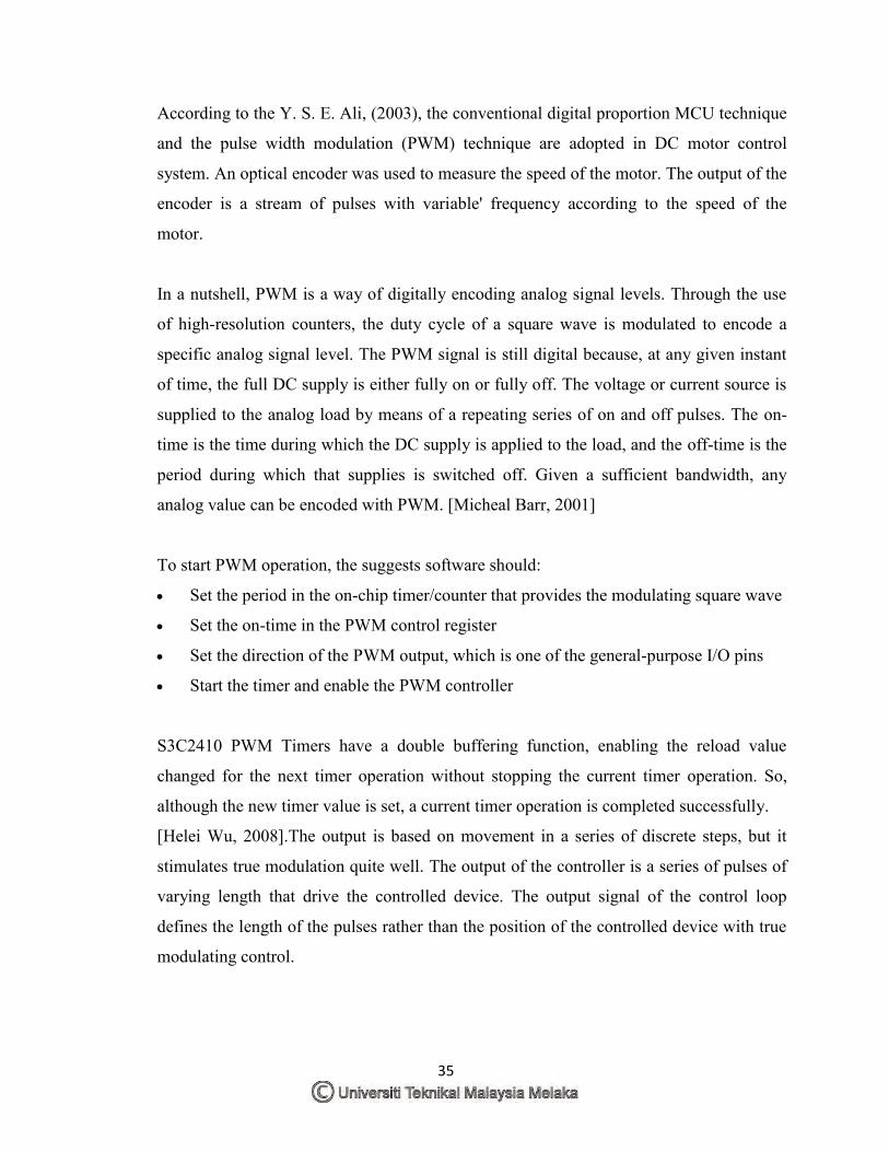
Robert Mcdowall ,(2004) state four types of pulse-width modulation (PWM) are possible:
1. The pulse center may be fixed in the center of the time window and both edges of the
pulse moved to compress or expand the width.
2. The lead edge can be held at the lead edge of the window and the tail edge modulated.
3. The tail edge can be fixed and the lead edge modulated.
4. The pulse repetition frequency can be varied by the signal, and the pulse width can be
constant. However, this method has a more-restricted range of average output than the
other three.
One of the advantages of PWM is that the signal remains digital all the way from the
processor to the controlled system, no digital-to-analog conversion is necessary. By
keeping the signal digital, noise effects are minimized. Noise can only affect a digital
signal if it is strong enough to change a logic-1 to a logic-0, or vice versa.
Increased noise immunity is yet another benefit of choosing PWM over analog control,
and is the principal reason PWM is sometimes used for communication. Switching from
an analog signal to PWM can increase the length of a communications channel
dramatically. At the receiving end, a suitable RC (resistor-capacitor) or LC (inductor-
capacitor) network can remove the modulating high frequency square wave and return the
signal to analog form.[ Robert Mcdowall, 2004].
Figure 2.10 : PWM signals of varying duty cycles [Michael Barr, 2001]
37
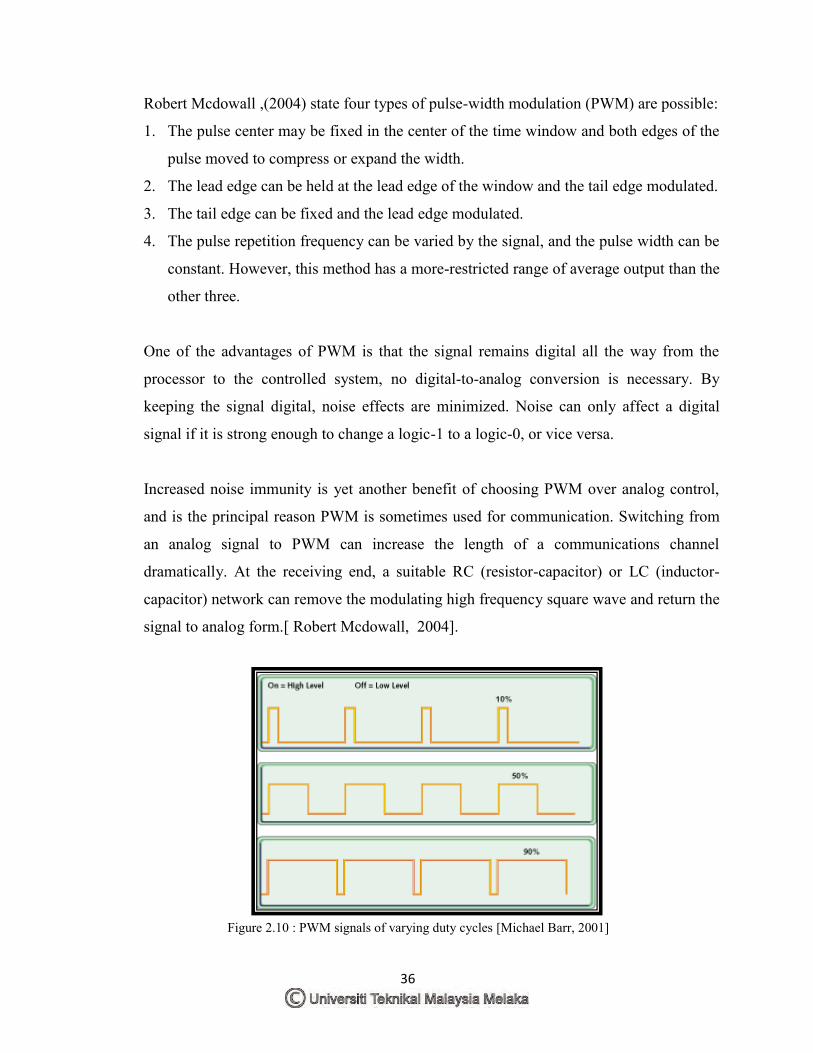
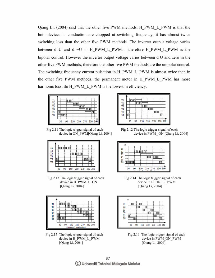
Qiang Li, (2004) said that the other five PWM methods, H_PWM_L_PWM is that the
both devices in conduction are chopped at switching frequency, it has almost twice
switching loss than the other five PWM methods. The inverter output voltage varies
between d U and d −U in H_PWM_L_PWM, therefore H_PWM_L_PWM is the
bipolar control. However the inverter output voltage varies between d U and zero in the
other five PWM methods, therefore the other five PWM methods are the unipolar control.
The switching frequency current pulsation in H_PWM_L_PWM is almost twice than in
the other five PWM methods, the permanent motor in H_PWM_L_PWM has more
harmonic loss. So H_PWM_L_PWM is the lowest in efficiency.
Fig 2.11 The logic trigger signal of each Fig 2.12 The logic trigger signal of each device in ON_PWM[Qiang Li, 2004] device in PWM_ ON [Qiang Li, 2004]
Fig 2.13 The logic trigger signal of each Fig 2.14 The logic trigger signal of each device in H_PWM_L_ON device in H_ON_L_ PWM [Qiang Li, 2004] [Qiang Li, 2004]
Fig 2.15 The logic trigger signal of each Fig 2.16 The logic trigger signal of each device in H_PWM_L_PWM device in PWM_ON_PWM [Qiang Li, 2004] [Qiang Li, 2004]
38
Because H_PWM_L_PWM has more switching loss, the demand to the inverter heat
dissipation performance is very high. The switching loss of each device is different in
H_PWM_L_ON and H_ON_L_PWM and temperature is not uniform in the heat sink
surface. According to the inverter heat dissipation performance, PWM_ON, ON_PWM
and PWM_ON_PWM have higher reliability than H_PWM_L_ON. It will cause the
H_ON_L_PWM has the same device logic trigger signal with ON_PWM from zero to
600 and with the PWM_ON from 600 to 1200 in the 1200 conduction mode. Therefore
the torque pulsation in H_PWM_L_ON and H_ON_L_PWM is larger than in PWM_ON
and ON_PWM.
2.8.2 Controlling Using H-Bridge
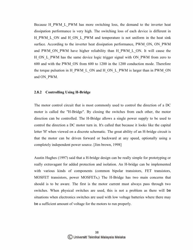
The motor control circuit that is most commonly used to control the direction of a DC
motor is called the "H-Bridge". By closing the switches from each other, the motor
direction can be controlled. The H-Bridge allows a single power supply to be used to
control the direction a DC motor turn in. It's called that because it looks like the capital
letter 'H' when viewed on a discrete schematic. The great ability of an H-bridge circuit is
that the motor can be driven forward or backward at any speed, optionally using a
completely independent power source. [Jim brown, 1998]
Austin Hughes (1997) said that a H-bridge design can be really simple for prototyping or
really extravagant for added protection and isolation. An H-bridge can be implemented
with various kinds of components (common bipolar transistors, FET transistors,
MOSFET transistors, power MOSFETs,) The H-Bridge has two main concerns that
should is to be aware. The first is the motor current must always pass through two
switches. When physical switches are used, this is not a problem as there will be
situations when electronics switches are used with low voltage batteries where there may
be a sufficient amount of voltage for the motors to run properly.
39
The second concern is quite suitable and is one that one must be aware at all the time. The
motors will turn when one switch on either side of the H-Bridge is closed. If both
switches on the same side of the H-Bridge are closed, it will be a problem, by closing the
two switches on the same side of the H-Bridge the short circuit will happened. This DC
motors up to about 100 watts or 5 amps or 40 volts, whichever comes first. Using bigger
parts could make it more powerful. Using a real H-bridge IC makes sense for this size of
motor. Operation is simple. Motor power is required, 6 to 40 volts DC. There are two
logic level compatible inputs, A and B, and two outputs, A and B. If input A is brought
high, output A goes high and output B goes low. [Tim A. Haskew, 1999].
The motor goes in one direction. If input B is driven, the opposite happens and the motor
runs in the opposite direction. If both inputs are low, the motor is not driven and can
freely "coast", and the circuit consumes no power. If both inputs are brought high, the
motor is shorted and braking occurs. This is a special feature of H-bridge designs.[ Bob
Jordan, 2002]
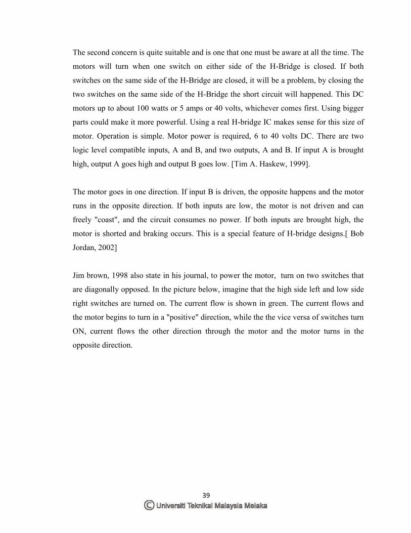
Jim brown, 1998 also state in his journal, to power the motor, turn on two switches that
are diagonally opposed. In the picture below, imagine that the high side left and low side
right switches are turned on. The current flow is shown in green. The current flows and
the motor begins to turn in a "positive" direction, while the the vice versa of switches turn
ON, current flows the other direction through the motor and the motor turns in the
opposite direction.
40
Figure 2.17 : H- bridge connection Figure 2.18 : Current through H-Bridge
[www.mcmanis.com] [www.mcmanis.com]
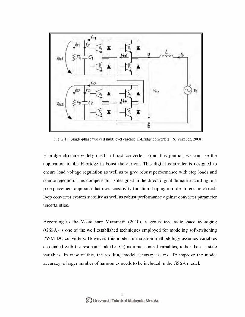
One of the applications of the H-bridge also apply in design a single phased multilevel of
two cell multilevel. The DC-Link voltages control problem is not a trivial issue in the
cascaded multilevel topology. As in other multilevel converters, the voltages control task
can be approached through modulation or as a part of the system controller. When the
modulation is used to control the output voltages, the redundant output states of the
converter are used. This fact is used to regulate the outputs voltages to the same reference
value. When the control approach is used, a specific control has to be designed to carry
out the voltages control task. [ S. Vazquez, 2008]
To analyze the controller design stages, the power exchange between the cells of a
cascade converter and the grid. The cells have been replaced by voltage sources with
values equal to the instantaneous voltages modulated by the cells, Vm1 and Vm2
respectively. The active and reactive power consumed or injected by each cell depend on
the shift angle between the current is, and the modulated voltage in the cell (Vm1). This
can be analyzed using the diagram of the cascade power converter
41
Fig. 2.19 Single-phase two cell multilevel cascade H-Bridge converter[.[ S. Vazquez, 2008]
H-bridge also are widely used in boost converter. From this journal, we can see the
application of the H-bridge in boost the current. This digital controller is designed to
ensure load voltage regulation as well as to give robust performance with step loads and
source rejection. This compensator is designed in the direct digital domain according to a
pole placement approach that uses sensitivity function shaping in order to ensure closed-
loop converter system stability as well as robust performance against converter parameter
uncertainties.
According to the Veerachary Mummadi (2010), a generalized state-space averaging
(GSSA) is one of the well established techniques employed for modeling soft-switching
PWM DC converters. However, this model formulation methodology assumes variables
associated with the resonant tank (Lr, Cr) as input control variables, rather than as state
variables. In view of this, the resulting model accuracy is low. To improve the model
accuracy, a larger number of harmonics needs to be included in the GSSA model.
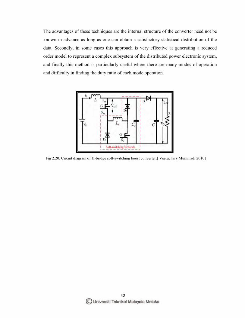
42
The advantages of these techniques are the internal structure of the converter need not be
known in advance as long as one can obtain a satisfactory statistical distribution of the
data. Secondly, in some cases this approach is very effective at generating a reduced
order model to represent a complex subsystem of the distributed power electronic system,
and finally this method is particularly useful where there are many modes of operation
and difficulty in finding the duty ratio of each mode operation.
Fig 2.20. Circuit diagram of H-bridge soft-switching boost converter.[ Veerachary Mummadi 2010]

43
2.9 Conclusion
Through this chapter, three important elements were separated in order to achieve the
objective for this project. An element is design an embedded system, control system
element and method for controlling a DC motor with application of microcontroller. For
designing an embedded system, information from previous project and journal has been
noted to look on how to develop an embedded system. From that journal, all design and
the way it designs has been noted in order to get some idea for design the embedded
system in chapter 4.
For control system element and method for controlling a DC motor, an experiment
conducted by the author in their journal has been noted. From the experiment,
information on handling the project and how to take a result has been discussed. The
information helps in identifying an appropriate method and design and handling the
project.
Finally, all information from this chapter has bringing it on to the next chapter which is
chapter 3 that can discussed the methodology for development of this project.
44
CHAPTER 3 METHODOLOGY
3.0 Introduction
The methodology will discuss the method for design and development of this project.
This method includes the flow chart process of the project and the flow chart of
embedded system for controlling a DC motor using microcontroller. Base on the
understanding research about embedded system implementation, the flow chart of the
process will be created. How to make the embedded system is the main of the flow chart
designated. Where the method to be done for the embedded system functionality with the
criteria based on the objective and scopes of the project. The flow chart will cover the
element in designing an embedded system for controlling a DC motor.
For the controller of DC motor, a microcontroller is used with addition of a control
system element which is PID. This PID algorithm will compensate the DC motor to
running at higher accuracy and less error. This PID is build from three term which is
P(Proportional), I(Integral) and D(Derivatives). Each component has their own capability
for controlling a DC motor. Kp can be used for increase the transient response of DC
motor. We can set some values of Kp until get a an optimum system response. For the Ki,
it were used for overcome the steady state error. Lastly, Kd is used to get a better
response in achieving a set point of the controller by entering a several value. This
chapter also will described
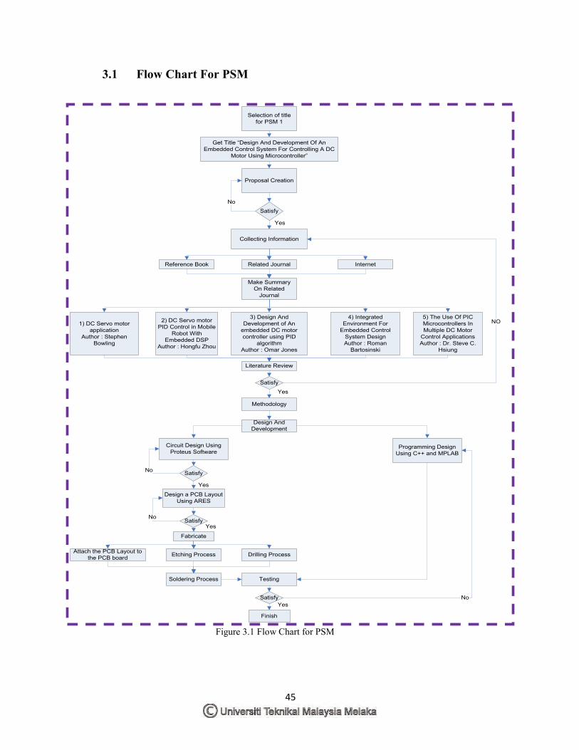
45
3.1 Flow Chart For PSM
Figure 3.1 Flow Chart for PSM
Selection of title for PSM 1
Get Title “Design And Development Of An Embedded Control System For Controlling A DC
Motor Using Microcontroller”
Proposal Creation
SatisfyNo
Collecting Information
Related JournalReference Book Internet
Make Summary On Related
Journal
1) DC Servo motor application
Author : Stephen Bowling
3) Design And Development of An
embedded DC motor controller using PID
algorithmAuthor : Omar Jones
2) DC Servo motor PID Control in Mobile
Robot With Embedded DSP
Author : Hongfu Zhou
4) Integrated Environment For
Embedded Control System DesignAuthor : Roman
Bartosinski
5) The Use Of PIC Microcontrollers In Multiple DC Motor
Control ApplicationsAuthor : Dr. Steve C.
Hsiung
Literature Review
Satisfy
NO
Yes
Methodology
Design And Development
Circuit Design Using Proteus Software
Programming Design Using C++ and MPLAB
Satisfy
Design a PCB Layout Using ARES
Satisfy
Fabricate
Etching Process Drilling ProcessAttach the PCB Layout to the PCB board
Soldering Process Testing
Satisfy
No
No
No
Finish
Yes
Yes
Yes
Yes
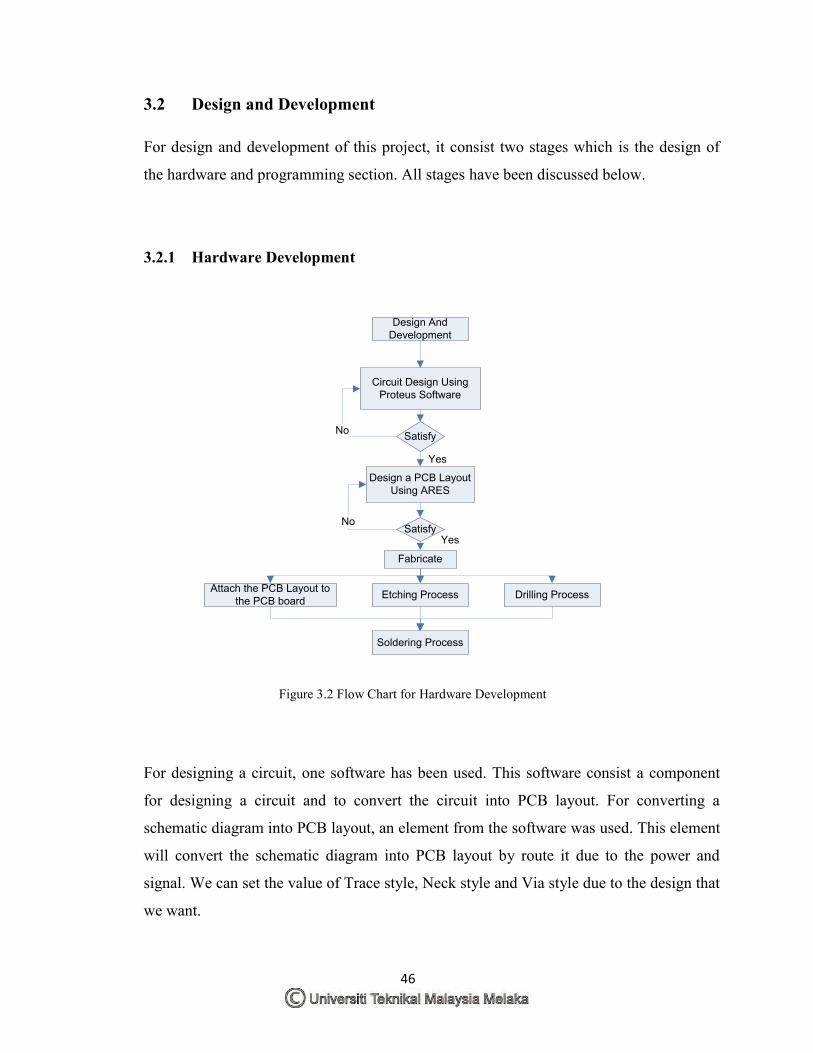
46
3.2 Design and Development
For design and development of this project, it consist two stages which is the design of
the hardware and programming section. All stages have been discussed below.
3.2.1 Hardware Development
Figure 3.2 Flow Chart for Hardware Development
For designing a circuit, one software has been used. This software consist a component
for designing a circuit and to convert the circuit into PCB layout. For converting a
schematic diagram into PCB layout, an element from the software was used. This element
will convert the schematic diagram into PCB layout by route it due to the power and
signal. We can set the value of Trace style, Neck style and Via style due to the design that
we want.
Design And Development
Circuit Design Using Proteus Software
Satisfy
Design a PCB Layout Using ARES
Satisfy
Fabricate
Etching Process Drilling ProcessAttach the PCB Layout to the PCB board
Soldering Process
No
No
Yes
Yes
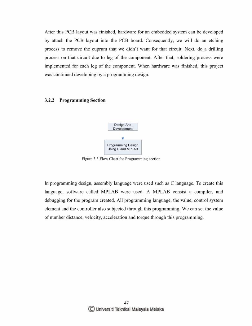
47
After this PCB layout was finished, hardware for an embedded system can be developed
by attach the PCB layout into the PCB board. Consequently, we will do an etching
process to remove the cuprum that we didn’t want for that circuit. Next, do a drilling
process on that circuit due to leg of the component. After that, soldering process were
implemented for each leg of the component. When hardware was finished, this project
was continued developing by a programming design.
3.2.2 Programming Section
Figure 3.3 Flow Chart for Programming section
In programming design, assembly language were used such as C language. To create this
language, software called MPLAB were used. A MPLAB consist a compiler, and
debugging for the program created. All programming language, the value, control system
element and the controller also subjected through this programming. We can set the value
of number distance, velocity, acceleration and torque through this programming.
Design And Development
Programming Design Using C and MPLAB
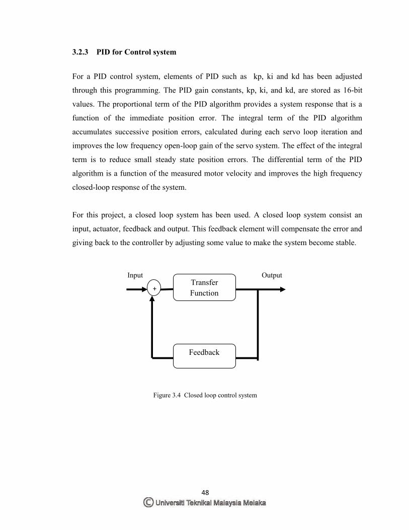
48
3.2.3 PID for Control system
For a PID control system, elements of PID such as kp, ki and kd has been adjusted
through this programming. The PID gain constants, kp, ki, and kd, are stored as 16-bit
values. The proportional term of the PID algorithm provides a system response that is a
function of the immediate position error. The integral term of the PID algorithm
accumulates successive position errors, calculated during each servo loop iteration and
improves the low frequency open-loop gain of the servo system. The effect of the integral
term is to reduce small steady state position errors. The differential term of the PID
algorithm is a function of the measured motor velocity and improves the high frequency
closed-loop response of the system.
For this project, a closed loop system has been used. A closed loop system consist an
input, actuator, feedback and output. This feedback element will compensate the error and
giving back to the controller by adjusting some value to make the system become stable.
Input Output
Figure 3.4 Closed loop control system
Transfer Function
Feedback
+
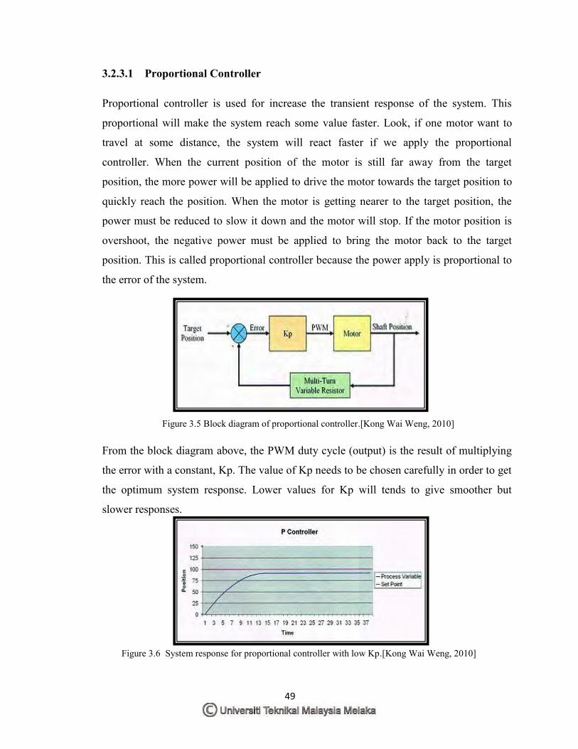
49
3.2.3.1 Proportional Controller Proportional controller is used for increase the transient response of the system. This
proportional will make the system reach some value faster. Look, if one motor want to
travel at some distance, the system will react faster if we apply the proportional
controller. When the current position of the motor is still far away from the target
position, the more power will be applied to drive the motor towards the target position to
quickly reach the position. When the motor is getting nearer to the target position, the
power must be reduced to slow it down and the motor will stop. If the motor position is
overshoot, the negative power must be applied to bring the motor back to the target
position. This is called proportional controller because the power apply is proportional to
the error of the system.
Figure 3.5 Block diagram of proportional controller.[Kong Wai Weng, 2010]
From the block diagram above, the PWM duty cycle (output) is the result of multiplying
the error with a constant, Kp. The value of Kp needs to be chosen carefully in order to get
the optimum system response. Lower values for Kp will tends to give smoother but
slower responses.
Figure 3.6 System response for proportional controller with low Kp.[Kong Wai Weng, 2010]
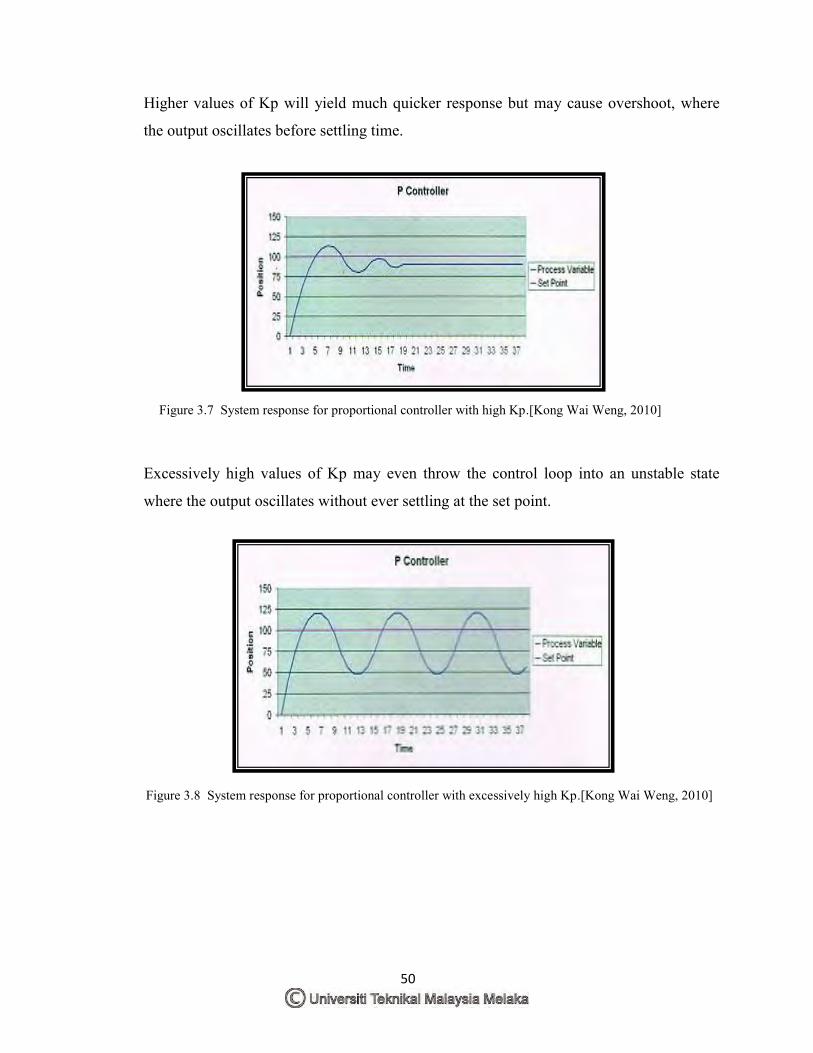
50
Higher values of Kp will yield much quicker response but may cause overshoot, where
the output oscillates before settling time.
Figure 3.7 System response for proportional controller with high Kp.[Kong Wai Weng, 2010]
Excessively high values of Kp may even throw the control loop into an unstable state
where the output oscillates without ever settling at the set point.
Figure 3.8 System response for proportional controller with excessively high Kp.[Kong Wai Weng, 2010]
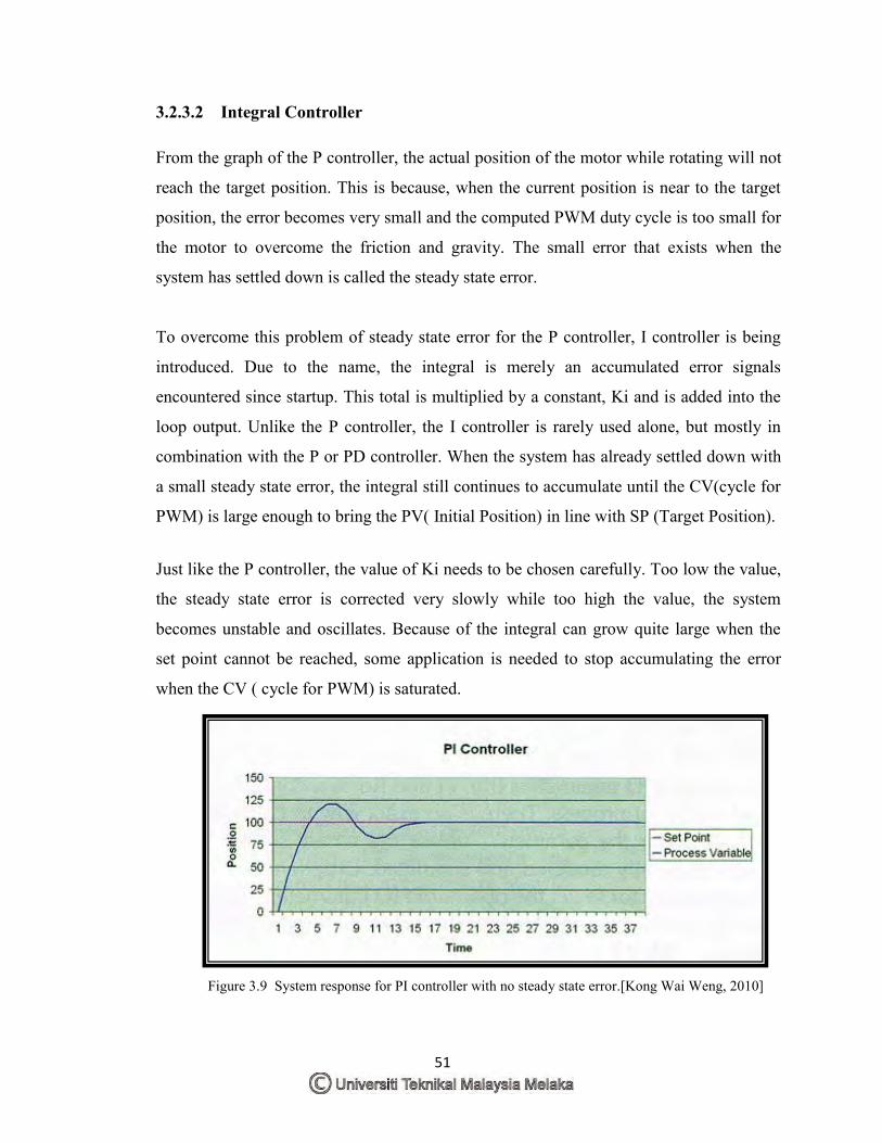
51
3.2.3.2 Integral Controller From the graph of the P controller, the actual position of the motor while rotating will not
reach the target position. This is because, when the current position is near to the target
position, the error becomes very small and the computed PWM duty cycle is too small for
the motor to overcome the friction and gravity. The small error that exists when the
system has settled down is called the steady state error.
To overcome this problem of steady state error for the P controller, I controller is being
introduced. Due to the name, the integral is merely an accumulated error signals
encountered since startup. This total is multiplied by a constant, Ki and is added into the
loop output. Unlike the P controller, the I controller is rarely used alone, but mostly in
combination with the P or PD controller. When the system has already settled down with
a small steady state error, the integral still continues to accumulate until the CV(cycle for
PWM) is large enough to bring the PV( Initial Position) in line with SP (Target Position).
Just like the P controller, the value of Ki needs to be chosen carefully. Too low the value,
the steady state error is corrected very slowly while too high the value, the system
becomes unstable and oscillates. Because of the integral can grow quite large when the
set point cannot be reached, some application is needed to stop accumulating the error
when the CV ( cycle for PWM) is saturated.
Figure 3.9 System response for PI controller with no steady state error.[Kong Wai Weng, 2010]
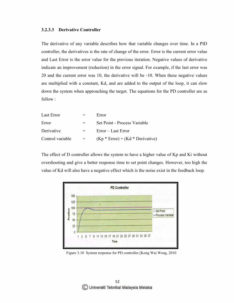
52
3.2.3.3 Derivative Controller
The derivative of any variable describes how that variable changes over time. In a PID
controller, the derivatives is the rate of change of the error. Error is the current error value
and Last Error is the error value for the previous iteration. Negative values of derivative
indicate an improvement (reduction) in the error signal. For example, if the last error was
20 and the current error was 10, the derivative will be -10. When these negative values
are multiplied with a constant, Kd, and are added to the output of the loop, it can slow
down the system when approaching the target. The equations for the PD controller are as
follow :
Last Error = Error
Error = Set Point - Process Variable
Derivative = Error – Last Error
Control variable = (Kp * Error) + (Kd * Derivative)
The effect of D controller allows the system to have a higher value of Kp and Ki without
overshooting and give a better response time to set point changes. However, too high the
value of Kd will also have a negative effect which is the noise exist in the feedback loop.
Figure 3.10 System response for PD controller.[Kong Wai Weng, 2010
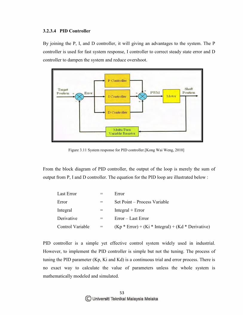
53
3.2.3.4 PID Controller By joining the P, I, and D controller, it will giving an advantages to the system. The P
controller is used for fast system response, I controller to correct steady state error and D
controller to dampen the system and reduce overshoot.
Figure 3.11 System response for PID controller.[Kong Wai Weng, 2010]
From the block diagram of PID controller, the output of the loop is merely the sum of
output from P, I and D controller. The equation for the PID loop are illustrated below :
Last Error = Error
Error = Set Point – Process Variable
Integral = Integral + Error
Derivative = Error – Last Error
Control Variable = (Kp * Error) + (Ki * Integral) + (Kd * Derivative)
PID controller is a simple yet effective control system widely used in industrial.
However, to implement the PID controller is simple but not the tuning. The process of
tuning the PID parameter (Kp, Ki and Kd) is a continuous trial and error process. There is
no exact way to calculate the value of parameters unless the whole system is
mathematically modeled and simulated.
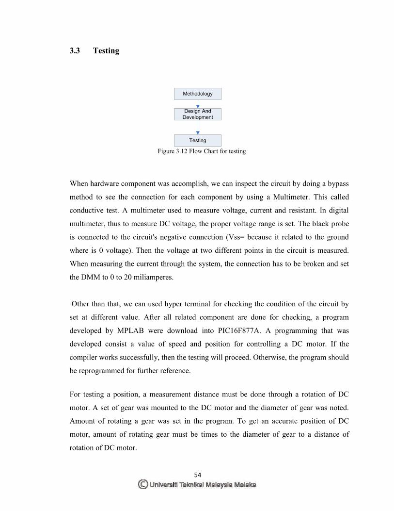
54
3.3 Testing
Figure 3.12 Flow Chart for testing
When hardware component was accomplish, we can inspect the circuit by doing a bypass
method to see the connection for each component by using a Multimeter. This called
conductive test. A multimeter used to measure voltage, current and resistant. In digital
multimeter, thus to measure DC voltage, the proper voltage range is set. The black probe
is connected to the circuit's negative connection (Vss= because it related to the ground
where is 0 voltage). Then the voltage at two different points in the circuit is measured.
When measuring the current through the system, the connection has to be broken and set
the DMM to 0 to 20 miliamperes.
Other than that, we can used hyper terminal for checking the condition of the circuit by
set at different value. After all related component are done for checking, a program
developed by MPLAB were download into PIC16F877A. A programming that was
developed consist a value of speed and position for controlling a DC motor. If the
compiler works successfully, then the testing will proceed. Otherwise, the program should
be reprogrammed for further reference.
For testing a position, a measurement distance must be done through a rotation of DC
motor. A set of gear was mounted to the DC motor and the diameter of gear was noted.
Amount of rotating a gear was set in the program. To get an accurate position of DC
motor, amount of rotating gear must be times to the diameter of gear to a distance of
rotation of DC motor.
Methodology
Design And Development
Testing
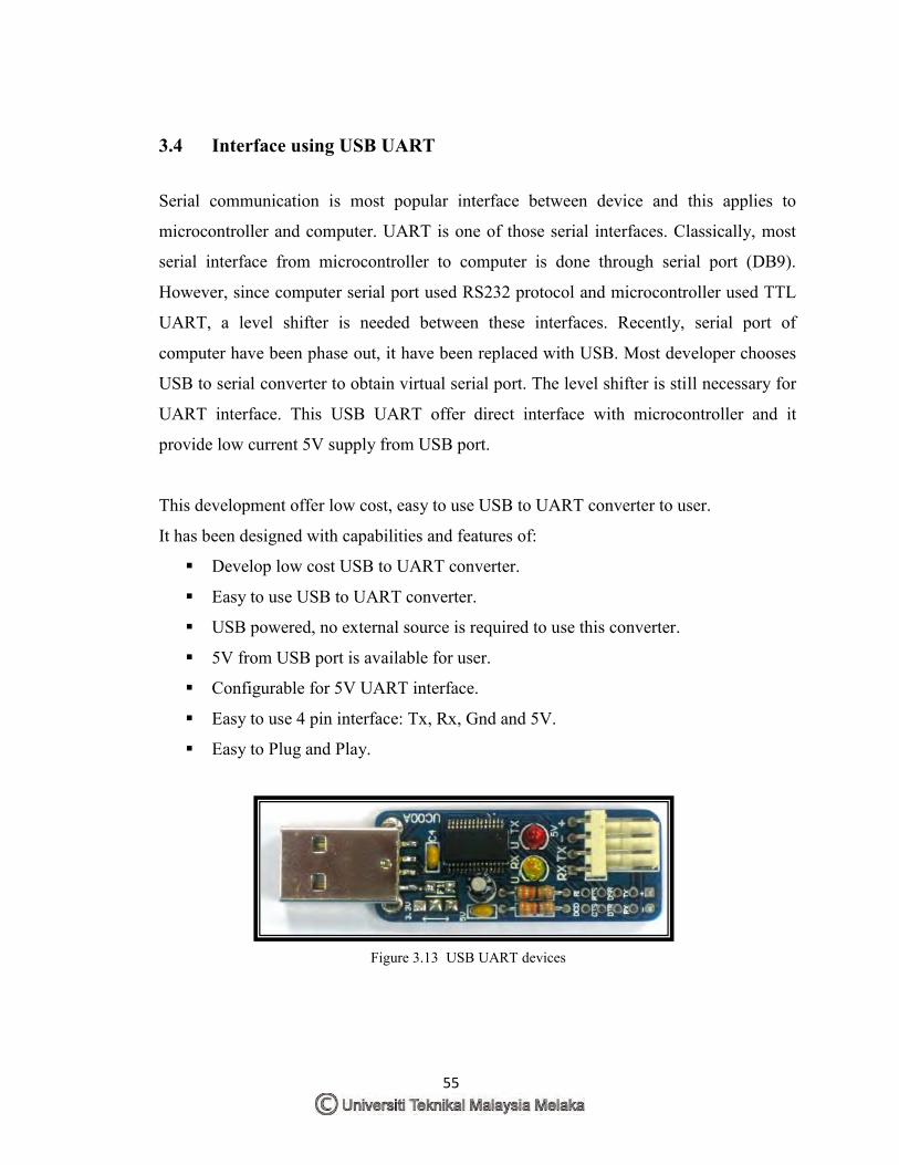
55
3.4 Interface using USB UART
Serial communication is most popular interface between device and this applies to
microcontroller and computer. UART is one of those serial interfaces. Classically, most
serial interface from microcontroller to computer is done through serial port (DB9).
However, since computer serial port used RS232 protocol and microcontroller used TTL
UART, a level shifter is needed between these interfaces. Recently, serial port of
computer have been phase out, it have been replaced with USB. Most developer chooses
USB to serial converter to obtain virtual serial port. The level shifter is still necessary for
UART interface. This USB UART offer direct interface with microcontroller and it
provide low current 5V supply from USB port.
This development offer low cost, easy to use USB to UART converter to user.
It has been designed with capabilities and features of:
Develop low cost USB to UART converter.
Easy to use USB to UART converter.
USB powered, no external source is required to use this converter.
5V from USB port is available for user.
Configurable for 5V UART interface.
Easy to use 4 pin interface: Tx, Rx, Gnd and 5V.
Easy to Plug and Play.
Figure 3.13 USB UART devices
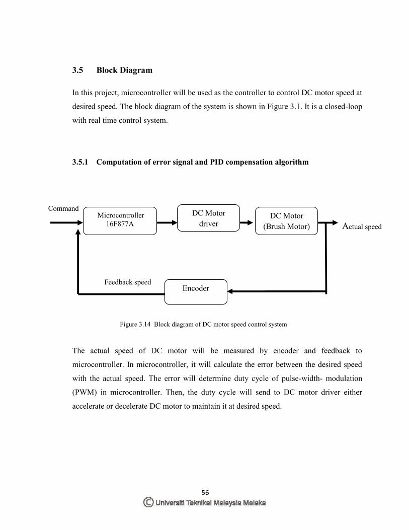
56
3.5 Block Diagram In this project, microcontroller will be used as the controller to control DC motor speed at
desired speed. The block diagram of the system is shown in Figure 3.1. It is a closed-loop
with real time control system.
3.5.1 Computation of error signal and PID compensation algorithm
Command
Actual speed
Feedback speed
Figure 3.14 Block diagram of DC motor speed control system
The actual speed of DC motor will be measured by encoder and feedback to
microcontroller. In microcontroller, it will calculate the error between the desired speed
with the actual speed. The error will determine duty cycle of pulse-width- modulation
(PWM) in microcontroller. Then, the duty cycle will send to DC motor driver either
accelerate or decelerate DC motor to maintain it at desired speed.
Microcontroller 16F877A
DC Motor driver
IC
DC Motor (Brush Motor)
Encoder
57
CHAPTER 4 DESIGN AND DEVELOPMENT
4.0 Background
This chapter focuses on the design and development of this project. This chapter also
will show and discuss the method on how to control a DC motor using a
microcontroller with some added value through a PID algorithm.
4.1 Flowchart
The flowchart in figure 4.1 showed that on how the design and development of an
embedded system for controlling a DC motor using a PID can be done. The flowchart
is continues from the previous chapter. On this chapter, the design was started with the
design of the schematic first. The schematic was designed using software called
Proteus. When schematic was completed, the design goes through to the programming
section.
In programming section, the program was build using software called MPLAB.
Through this software, all instruction and coding to controlled a motor was specified
together with a PID algorithm. Build this program on MPLAB to get the Hex file.
Attach the hex file to the PIC in schematic design and try simulating. If successful, the
DC motor will rotate due to the value that is inserted by the user.
58
To create a PCB layout, the schematic design in Proteus must be converted. This can
be done by using an Ares element in proteus. All components must be specified and
the path along component will automatically created by software. Get a PCB layout by
saving the work into bitmap image and do a hardware development. In the hardware
development, there are three stages that must be completed which is etching, drilling
and soldering process. After this process was done, the completed circuit can be
verified and testing.
Through a testing section, there several stage that must be done in completing this
project. First stage of testing is conductive test. This test allows the user to identify the
current path that is connected or vice versa. Secondly, testing should be done in
interface section. This project used a UART serial communication in order to interface
the project with the laptop. This UART contain a transmit (TX) and receive (RX) port
to make it able to send a signal between laptop and project. This serial communication
can be done using software called X-CTU. Through this software, it will display a
command and all value can be entered and will send to the project via UART. The
encoder of the motor will be triggered and the DC motor wills rotated due to the value
that are entered by the user.
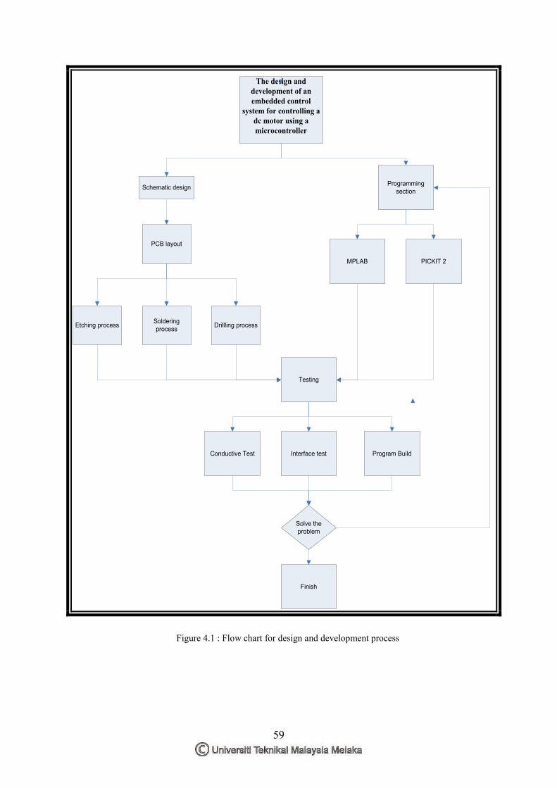
59
The design and development of an embedded control
system for controlling a dc motor using a microcontroller
Schematic design Programming section
PCB layout
Etching process Soldering process Drillling process
Testing
MPLAB PICKIT 2
Conductive Test Interface test Program Build
Solve the problem
Finish
Figure 4.1 : Flow chart for design and development process
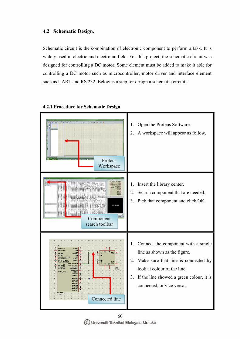
60
4.2 Schematic Design.
Schematic circuit is the combination of electronic component to perform a task. It is
widely used in electric and electronic field. For this project, the schematic circuit was
designed for controlling a DC motor. Some element must be added to make it able for
controlling a DC motor such as microcontroller, motor driver and interface element
such as UART and RS 232. Below is a step for design a schematic circuit:-
4.2.1 Procedure for Schematic Design
1. Open the Proteus Software.
2. A workspace will appear as follow.
1. Insert the library center.
2. Search component that are needed.
3. Pick that component and click OK.
1. Connect the component with a single
line as shown as the figure.
2. Make sure that line is connected by
look at colour of the line.
3. If the line showed a green colour, it is
connected, or vice versa.
Proteus Workspace
Component search toolbar
Connected line
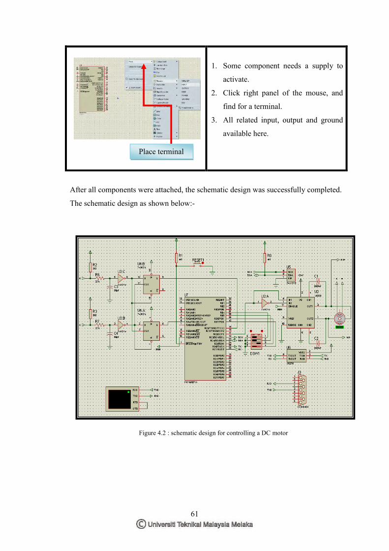
61
After all components were attached, the schematic design was successfully completed.
The schematic design as shown below:-
Figure 4.2 : schematic design for controlling a DC motor
1. Some component needs a supply to
activate.
2. Click right panel of the mouse, and
find for a terminal.
3. All related input, output and ground
available here.
Place terminal
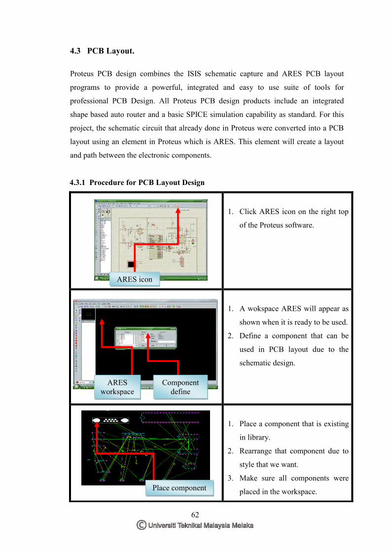
62
4.3 PCB Layout.
Proteus PCB design combines the ISIS schematic capture and ARES PCB layout
programs to provide a powerful, integrated and easy to use suite of tools for
professional PCB Design. All Proteus PCB design products include an integrated
shape based auto router and a basic SPICE simulation capability as standard. For this
project, the schematic circuit that already done in Proteus were converted into a PCB
layout using an element in Proteus which is ARES. This element will create a layout
and path between the electronic components.
4.3.1 Procedure for PCB Layout Design
1. Click ARES icon on the right top
of the Proteus software.
1. A wokspace ARES will appear as
shown when it is ready to be used.
2. Define a component that can be
used in PCB layout due to the
schematic design.
1. Place a component that is existing
in library.
2. Rearrange that component due to
style that we want.
3. Make sure all components were
placed in the workspace.
ARES icon
ARES workspace
Place component
Component define
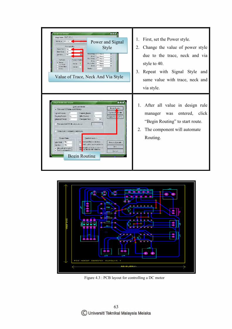
63
Figure 4.3 : PCB layout for controlling a DC motor
1. First, set the Power style.
2. Change the value of power style
due to the trace, neck and via
style to 40.
3. Repeat with Signal Style and
same value with trace, neck and
via style.
1. After all value in design rule
manager was entered, click
“Begin Routing” to start route.
2. The component will automate
Routing.
Power and Signal Style
Value of Trace, Neck And Via Style
Begin Routing
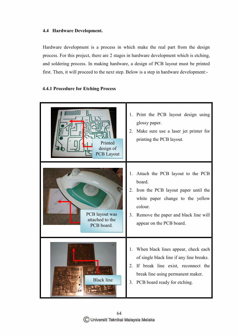
64
4.4 Hardware Development.
Hardware development is a process in which make the real part from the design
process. For this project, there are 2 stages in hardware development which is etching,
and soldering process. In making hardware, a design of PCB layout must be printed
first. Then, it will proceed to the next step. Below is a step in hardware development:-
4.4.1 Procedure for Etching Process
1. Print the PCB layout design using
glossy paper.
2. Make sure use a laser jet printer for
printing the PCB layout.
1. Attach the PCB layout to the PCB
board.
2. Iron the PCB layout paper until the
white paper change to the yellow
colour.
3. Remove the paper and black line will
appear on the PCB board.
1. When black lines appear, check each
of single black line if any line breaks.
2. If break line exist, reconnect the
break line using permanent maker.
3. PCB board ready for etching.
Printed design of
PCB Layout
PCB layout was attached to the
PCB board.
Black line
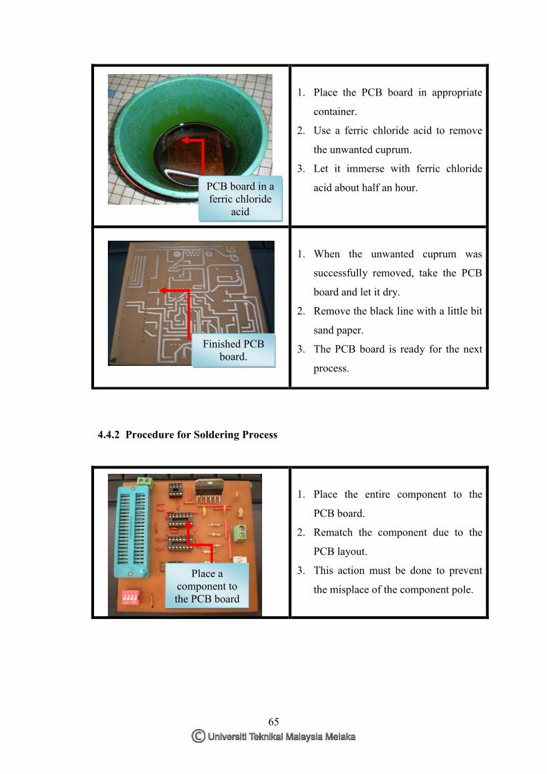
65
4.4.2 Procedure for Soldering Process
1. Place the PCB board in appropriate
container.
2. Use a ferric chloride acid to remove
the unwanted cuprum.
3. Let it immerse with ferric chloride
acid about half an hour.
1. When the unwanted cuprum was
successfully removed, take the PCB
board and let it dry.
2. Remove the black line with a little bit
sand paper.
3. The PCB board is ready for the next
process.
1. Place the entire component to the
PCB board.
2. Rematch the component due to the
PCB layout.
3. This action must be done to prevent
the misplace of the component pole.
PCB board in a ferric chloride
acid
Finished PCB board.
Place a component to the PCB board
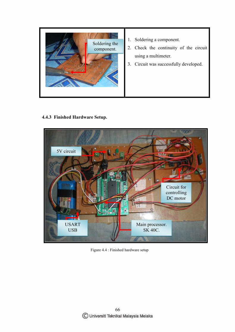
66
4.4.3 Finished Hardware Setup.
Figure 4.4 : Finished hardware setup
1. Soldering a component.
2. Check the continuity of the circuit
using a multimeter.
3. Circuit was successfully developed.
Soldering the component.
5V circuit
Circuit for controlling DC motor
Main processor. SK 40C.
USART USB
67
4.5 Designing PID Controller.
PID controller is one of the most popular controllers in control system application that
has been used to increase the transient response and reduce or eliminate the steady
state error that exist on the system. This project need a PID controller because when a
DC motor rotate and want to reach some position, with proportional gain, it will
increase the transient response and make the DC motor reach some position faster.
While, integral gain will reduce the steady state error that exists on the system.
Derivative is rate of the error that must be adjusting to make the system more stable
and can perform any task with minimum or no error exists.
There several consideration must be taken is designing a PID controller. One of that is
root locus graphic that showed the value of the gain, dominant poles, poles, and zeros.
The root locus typically allows us to choose the proper loop gain to meet a transient
response specification. As the gain is varied, we move through different regions of
response. Setting the gain at a particular value yields the transient response dictated by
the poles at that point on the root locus. Thus, we are limited to those responses that
exist along the root locus.
Flexibility in the design of a desired transient response can be increased if we can
design for transient response that is not on the root locus. In designing a PID
controller, we must create a compensator to increase the transient response.
Compensators are not only used to improve the transient response of a system, but it
also used independently to improve the steady state error characteristic. When the
system gain was adjusted to meet the transient response specification, steady state
error performance deteriorated, since both the transient response and the static error
constant were related to the gain. The higher the gain, the smaller the steady state
error, but the larger percent overshoot.
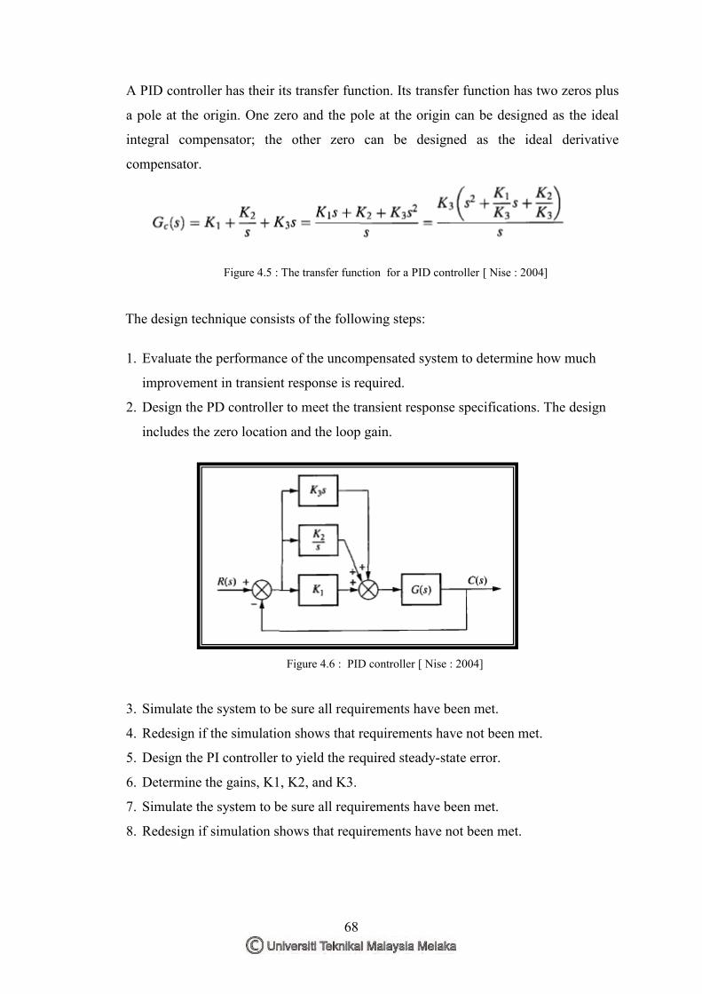
68
A PID controller has their its transfer function. Its transfer function has two zeros plus
a pole at the origin. One zero and the pole at the origin can be designed as the ideal
integral compensator; the other zero can be designed as the ideal derivative
compensator.
Figure 4.5 : The transfer function for a PID controller [ Nise : 2004]
The design technique consists of the following steps:
1. Evaluate the performance of the uncompensated system to determine how much
improvement in transient response is required.
2. Design the PD controller to meet the transient response specifications. The design
includes the zero location and the loop gain.
Figure 4.6 : PID controller [ Nise : 2004]
3. Simulate the system to be sure all requirements have been met.
4. Redesign if the simulation shows that requirements have not been met.
5. Design the PI controller to yield the required steady-state error.
6. Determine the gains, K1, K2, and K3.
7. Simulate the system to be sure all requirements have been met.
8. Redesign if simulation shows that requirements have not been met.
69
4.6 Programming Section
The main for this project is the way to control the DC motor using a microcontroller.
When say it about microcontroller, it is all about the programming. Programming will
let the user plan and specify some instruction to make the flow of the process going
smoothly and meet the requirement. Programming is a set of instruction in order to
define and do a related task due to the user. This project required a PID instruction to
control the rotation of the DC motor. We should define the value of Kp, Ki, and Kd in
order to control the DC motor and make it reach some position faster. Below is some
consideration should be taken in design a PID controller for a program and the way the
value of Kp, Ki, and Kd can control the rotation of DC motor. For this project, all
related programming was design and build up in software called MPLAB. This
software will let the user plan and specify the programming and will download the
programmed directly to the microcontroller.
4.6.1 Servo Calculation.
The entire servomotor function is implemented in the Interrupt Service Routine (ISR),
which must perform the following tasks:
• Get current motor position
• Get desired motor position
• Find the position error
• Determine new PWM duty cycle
Timer2, the time base for the CCP1 module, is used to generate interrupts that time the
servo calculations. This ensures that the PWM duty cycle changes are synchronous
with the PWM period. The frequency of the PWM signal that drives the motor should
be high enough so that a minimal amount of current ripple is induced in the windings
of the DC motor. The amount of current ripple can be derived from the PWM
frequency, motor winding resistance, and motor inductance. For this application, the
MCU is operated at 20 MHz and the PWM frequency is 19.53 kHz. At this PWM
frequency, a Timer2 interrupt would occur every 51 μs.
70
4.6.1.1 Position Updates The first task to be done in the servo calculations is to determine exactly where the
motor is at the present moment. The function UpdPos () is called to get the new motor
position. As mentioned earlier, Timer0 and Timer1 are used to accumulate the up and
down pulses that are derived from the encoder output signals. The counters are never
cleared to avoid the possibility of losing count information. Instead, the values of the
Timer0 and Timer1 registers saved during the previous sample period are subtracted
from the present timer values, using two's complement signed arithmetic.
The use of two's-complement arithmetic, also accounts for a timer overflow that may
have occurred since the last read. The down pulse count, DnCount, is then subtracted
from UpCount, the up pulse count, which provides a signed result indicating the total
distance traveled during the sample period. This value also represents the measured
velocity of the motor in encoder counts per servo update period and is stored in the
variable mvelocity.
The measured position of the motor is stored in the variable mposition. The upper 24
bits of mposition holds the position of the motor in encoder counts. The lower 8 bits
of mposition represent fractional encoder counts. The value of mvelocity is added to
mposition to find the new position of the motor. With 24 bits, the absolute position of
the motor may be tracked through 33,554 shaft revolutions using a 500 CPR encoder.
4.6.1.2 Error Calculation The CalcError() function subtracts the measured motor position, mposition, from the
commanded motor position in the variable position, to find the amount of position
error. The position error result is shifted to the right and the lower 8 bits that hold
fractional data are discarded. This leaves the 24-bit position error result, which is then
truncated to a 16-bit signed value for subsequent calculations.
71
4.6.1.3 Trajectory Updates. The commanded motor position is stored in the variable position. When the value of
position is constant, the motor shaft will be held in a fixed position. The fractional bits
in position allow the motor to be operated at very low velocities. In order for the
servomotor to produce smooth motion, a motion profile algorithm was needed to
controls the speed and acceleration of the motor. The UpdTraj( ) function does this
job and its purpose is to determine the next required value for position, based on the
current motion profile parameters. For this application, a movement distance, velocity
limit, and acceleration value are required to execute the profile.
The motion profile is executed in two phases. The first half of the movement distance
is traveled in the first phase and the remaining distance in the second phase. The
stat.phase flag indicates the current phase of the motion segment. Half of the total
distance to be traveled is stored in the variable phase1dist. The final destination
position for the motor is stored in fposition. The velocity limit for the motion profile is
stored in the variable vlim. The present commanded velocity of the motor is stored in
velact. The acceleration value for the profile is stored in accel. A delay time for the
motion profile is stored in the variable dtime. This variable tells the motion profile
how many servo update periods to wait before executing the next motion segment.
Finally, the direction of motion is set by the stat.neg_move flag.
The motor can be run at any desired speed by adding a value to position at each servo
update is stored in the variable velact. Furthermore, the motor will accelerate (or
decelerate) at a constant rate, if we add or subtract a value to velact at each servo
update. The acceleration value for the profile is stored in the variable accel. The value
of accel is added to velact at each servo update. The value of velact is then added or
subtracted from the commanded motor position, position, depending on the state of the
stat.neg_move flag. The value of velact is also subtracted from phase1dist to keep
track of the distance traveled in the first half of the move. The motor stops accelerating
when velact is greater than vlim. After the velocity limit has been reached, flatcount is
incremented at each servo update period to maintain the number of servo updates for
which no acceleration occurred.
72
4.6.1.4 Duty Cycle Calculations. The CalcPID( ) function implements a proportional – integral - derivative (PID)
compensator algorithm and uses the 16-bit error result to determine the next required
PWM duty cycle value. The PID gain constants kp, ki, and kd, are stored as 16-bit
values.
The proportional term of the PID algorithm provides a system response that is a
function of the immediate position error. The integral term of the PID algorithm
accumulates successive position errors, calculated during each servo loop iteration and
improves the low frequency open-loop gain of the servo system. The effect of the
integral term is to reduce small steady state position errors. The differential term of the
PID algorithm is a function of the measured motor velocity, mvelocity, and improves
the high frequency closed-loop response of the servo system.
After the three terms of the PID algorithm are summed, the 32-bit result stored in ypid
is saturated to 24 bits. The upper 16 bits of ypid are used to set the duty cycle, which
effectively divides the output of the PID algorithm by 256. Since the PWM module
has a 10-bit resolution, the value in the upper 16 bits of ypid is checked to see if it
exceeds +511 or -512. When this condition occurs, the PWM duty cycle is set to the
maximum positive or negative limit and the stat.saturated flag is set.
The integral accumulation in the PID algorithm is bypassed. This allows the
servomotor to smoothly resume motion when the saturation condition ends. If the
integral error and the motion profile continued to update, the servomotor would
produce sudden and erratic motions when recovering from a mechanical overload.
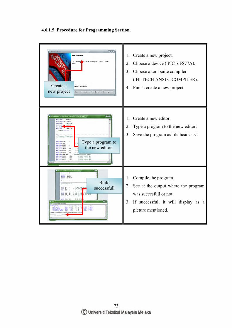
73
4.6.1.5 Procedure for Programming Section.
1. Create a new project.
2. Choose a device ( PIC16F877A).
3. Choose a tool suite compiler
( HI TECH ANSI C COMPILER).
4. Finish create a new project.
1. Create a new editor.
2. Type a program to the new editor.
3. Save the program as file header .C
1. Compile the program.
2. See at the output where the program
was succesfull or not.
3. If successful, it will display as a
picture mentioned.
Create a new project
Type a program to the new editor.
Build successfull
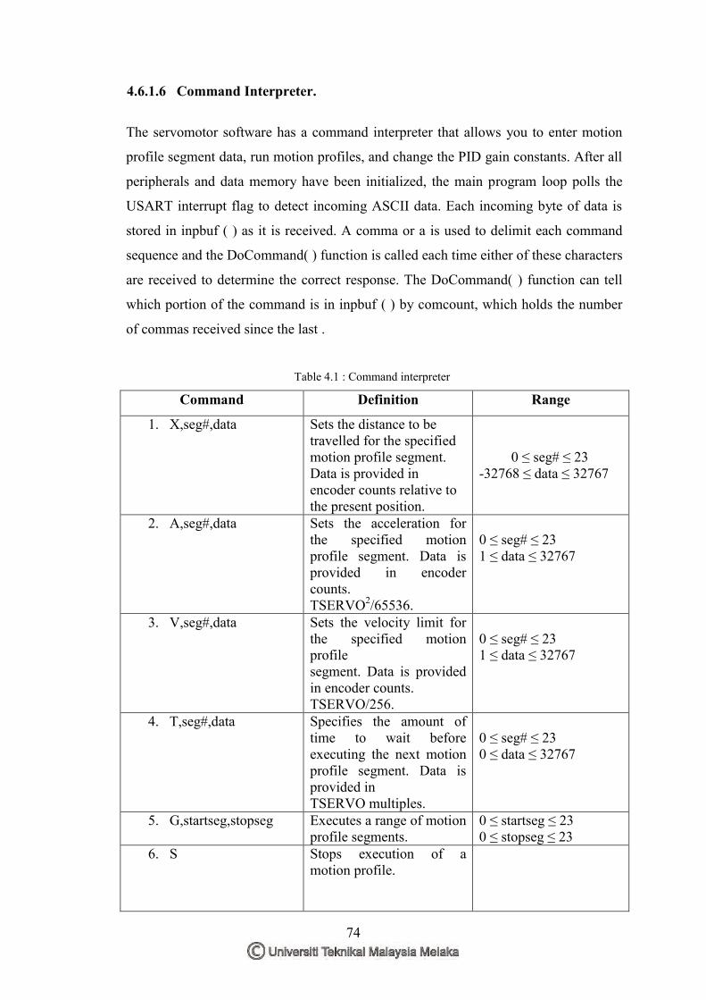
74
4.6.1.6 Command Interpreter.
The servomotor software has a command interpreter that allows you to enter motion
profile segment data, run motion profiles, and change the PID gain constants. After all
peripherals and data memory have been initialized, the main program loop polls the
USART interrupt flag to detect incoming ASCII data. Each incoming byte of data is
stored in inpbuf ( ) as it is received. A comma or a is used to delimit each command
sequence and the DoCommand( ) function is called each time either of these characters
are received to determine the correct response. The DoCommand( ) function can tell
which portion of the command is in inpbuf ( ) by comcount, which holds the number
of commas received since the last .
Table 4.1 : Command interpreter
Command Definition Range
1. X,seg#,data Sets the distance to be travelled for the specified motion profile segment. Data is provided in encoder counts relative to the present position.
0 ≤ seg# ≤ 23 -32768 ≤ data ≤ 32767
2. A,seg#,data
Sets the acceleration for the specified motion profile segment. Data is provided in encoder counts. TSERVO2/65536.
0 ≤ seg# ≤ 23 1 ≤ data ≤ 32767
3. V,seg#,data
Sets the velocity limit for the specified motion profile segment. Data is provided in encoder counts. TSERVO/256.
0 ≤ seg# ≤ 23 1 ≤ data ≤ 32767
4. T,seg#,data
Specifies the amount of time to wait before executing the next motion profile segment. Data is provided in TSERVO multiples.
0 ≤ seg# ≤ 23 0 ≤ data ≤ 32767
5. G,startseg,stopseg Executes a range of motion profile segments.
0 ≤ startseg ≤ 23 0 ≤ stopseg ≤ 23
6. S
Stops execution of a motion profile.
75
7. P,data
Changes the proportional gain for the PID algorithm.
-32768 ≤ data ≤ 32767
8. I,data
Changes the integral gain for the PID algorithm.
-32768 ≤ data ≤ 32767
9. D,data
Changes the differential gain for the PID algorithm.
-32768 ≤ data ≤ 32767
10. W
Enables or disables the PWM driver stage.
4.6.1.7 Stand Alone Operation.
The provided application firmware allows the servomotor to perform a few basic
motions without a PC connected. Specifically, data for three different motion profiles
are stored in the MCU program memory and are loaded into data memory at start-up.
Each profile is selected by turning on DIP switch #2, #3, or #4, connected to PORTB
and pressing the MCLR button. The software polls the DIP switches once, at start-up,
to see if a profile should be executed. The selected profile will begin to execute
immediately. If DIP switch #1 is turned on in combination with one of the other
switches, the selected profile will execute repeatedly.
76
CHAPTER 5 RESULT AND DISCUSSION
5.0 Background This chapter will focus on the result of the design and development of an embedded
control system for controlling a DC motor using microcontroller. A microcontroller
has chosen for this project because of its wide variety in performing task. In general,
this microcontroller will received a command signal from the user through interface
section using USART. Then, this microcontroller will interpret that data to perform a
task based to the given value entered by the user.
5.1 Result.
For this project, the result will mainly focus on several expectations through the
objective of this project.
Below are some expectations or results for this project:-
1. Successfully in design and development an embedded control system.
2. Study a control system element which is (PID) in controlling a DC motor.
3. Design a PID controller
4. Get an exact position during rotating of DC motor.
5. Make a comparison with real time application and simulation application based on
the time, and distance.
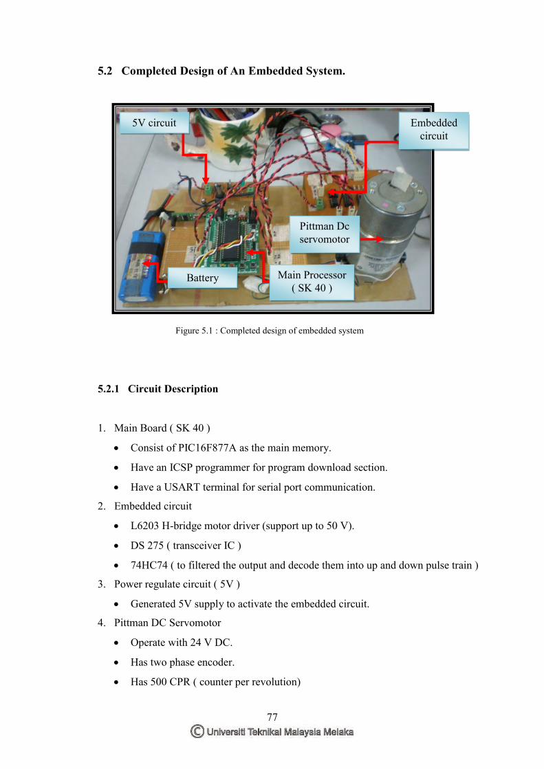
77
5.2 Completed Design of An Embedded System.
Figure 5.1 : Completed design of embedded system
5.2.1 Circuit Description
1. Main Board ( SK 40 )
Consist of PIC16F877A as the main memory.
Have an ICSP programmer for program download section.
Have a USART terminal for serial port communication.
2. Embedded circuit
L6203 H-bridge motor driver (support up to 50 V).
DS 275 ( transceiver IC )
74HC74 ( to filtered the output and decode them into up and down pulse train )
3. Power regulate circuit ( 5V )
Generated 5V supply to activate the embedded circuit.
4. Pittman DC Servomotor
Operate with 24 V DC.
Has two phase encoder.
Has 500 CPR ( counter per revolution)
5V circuit
Main Processor ( SK 40 )
Embedded circuit
Pittman Dc servomotor
Battery
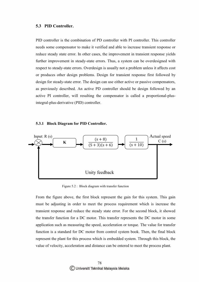
78
5.3 PID Controller.
PID controller is the combination of PD controller with PI controller. This controller
needs some compensator to make it verified and able to increase transient response or
reduce steady state error. In other cases, the improvement in transient response yields
further improvement in steady-state errors. Thus, a system can be overdesigned with
respect to steady-state errors. Overdesign is usually not a problem unless it affects cost
or produces other design problems. Design for transient response first followed by
design for steady-state error. The design can use either active or passive compensators,
as previously described. An active PD controller should be design followed by an
active PI controller, will resulting the compensator is called a proportional-plus-
integral-plus-derivative (PID) controller.
5.3.1 Block Diagram for PID Controller.
Input: R (s) Actual speed C (s)
Unity feedback
Figure 5.2 : Block diagram with transfer function
From the figure above, the first block represent the gain for this system. This gain
must be adjusting in order to meet the process requirement which is increase the
transient response and reduce the steady state error. For the second block, it showed
the transfer function for a DC motor. This transfer represents the DC motor in some
application such as measuring the speed, acceleration or torque. The value for transfer
function is a standard for DC motor from control system book. Then, the final block
represent the plant for this process which is embedded system. Through this block, the
value of velocity, acceleration and distance can be entered to meet the process plant.
K
(s + 8)
(S + 3) s + 6
1
(s + 10)
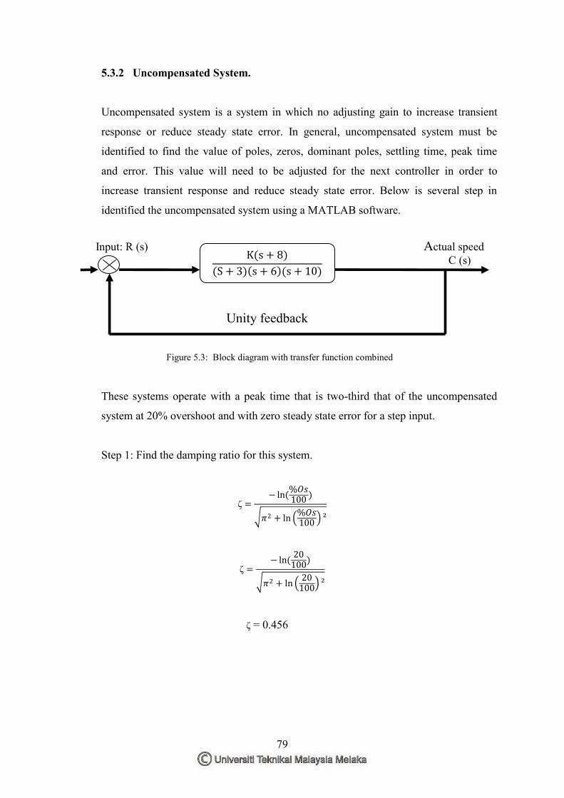
79
5.3.2 Uncompensated System.
Uncompensated system is a system in which no adjusting gain to increase transient
response or reduce steady state error. In general, uncompensated system must be
identified to find the value of poles, zeros, dominant poles, settling time, peak time
and error. This value will need to be adjusted for the next controller in order to
increase transient response and reduce steady state error. Below is several step in
identified the uncompensated system using a MATLAB software.
Input: R (s) Actual speed C (s)
Unity feedback
Figure 5.3: Block diagram with transfer function combined
These systems operate with a peak time that is two-third that of the uncompensated
system at 20% overshoot and with zero steady state error for a step input.
Step 1: Find the damping ratio for this system.
ζ =− ln(
%𝑂𝑠100
)
𝜋2 + ln %𝑂𝑠100
²
ζ =− ln(
20100
)
𝜋2 + ln 20
100 ²
ζ = 0.456
K(s + 8)
(S + 3) s + 6 (s + 10)
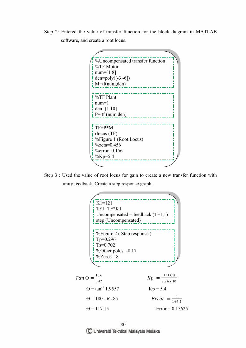
80
Step 2: Entered the value of transfer function for the block diagram in MATLAB
software, and create a root locus.
Step 3 : Used the value of root locus for gain to create a new transfer function with
unity feedback. Create a step response graph.
𝑇𝑎𝑛 Ө =10.6
5.42 𝐾𝑝 =
121 (8)
3 𝑥 6 𝑥 10
Ө = tan-1 1.9557 Kp = 5.4
Ө = 180 - 62.85 𝐸𝑟𝑟𝑜𝑟 =1
1+5.4
Ө = 117.15 Error = 0.15625
%Uncompensated transfer function %TF Motor num=[1 8] den=poly([-3 -6]) M=tf(num,den) %TF Plant num=1 den=[1 10] P= tf (num,den) TF=P*M rlocus (TF) %Figure 1 (Root Locus) %zeta=0.456 %error=0.156 %Kp=5.4
K1=121 TF1=TF*K1 Uncompensated = feedback (TF1,1) step (Uncompensated) %Figure 2 ( Step response ) Tp=0.296 Ts=0.702 %Other poles=-8.17 %Zeros=-8
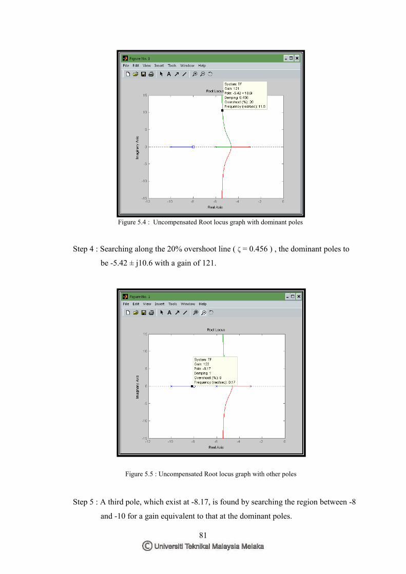
81
Figure 5.4 : Uncompensated Root locus graph with dominant poles
Step 4 : Searching along the 20% overshoot line ( ζ = 0.456 ) , the dominant poles to
be -5.42 ± j10.6 with a gain of 121.
Figure 5.5 : Uncompensated Root locus graph with other poles
Step 5 : A third pole, which exist at -8.17, is found by searching the region between -8
and -10 for a gain equivalent to that at the dominant poles.
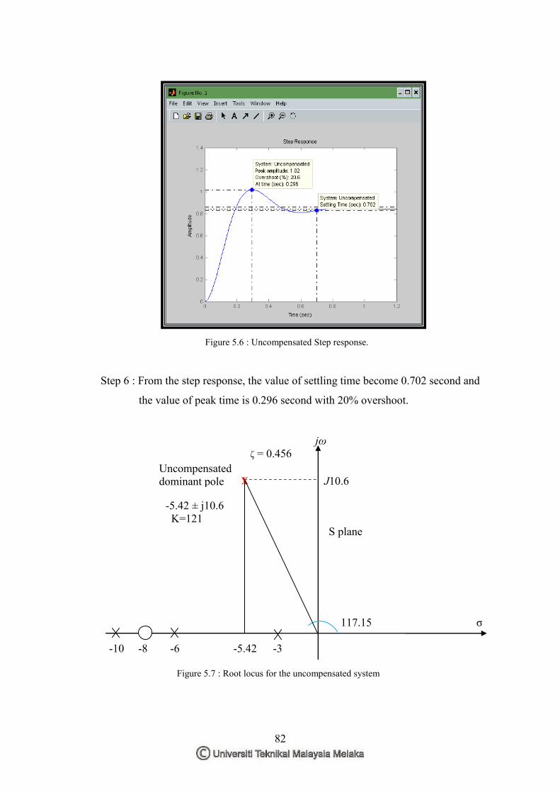
82
Figure 5.6 : Uncompensated Step response.
Step 6 : From the step response, the value of settling time become 0.702 second and
the value of peak time is 0.296 second with 20% overshoot.
jω ζ = 0.456 -5.42 ± j10.6 K=121 S plane 117.15 σ -10 -8 -6 -5.42 -3 Figure 5.7 : Root locus for the uncompensated system
x Uncompensated dominant pole J10.6
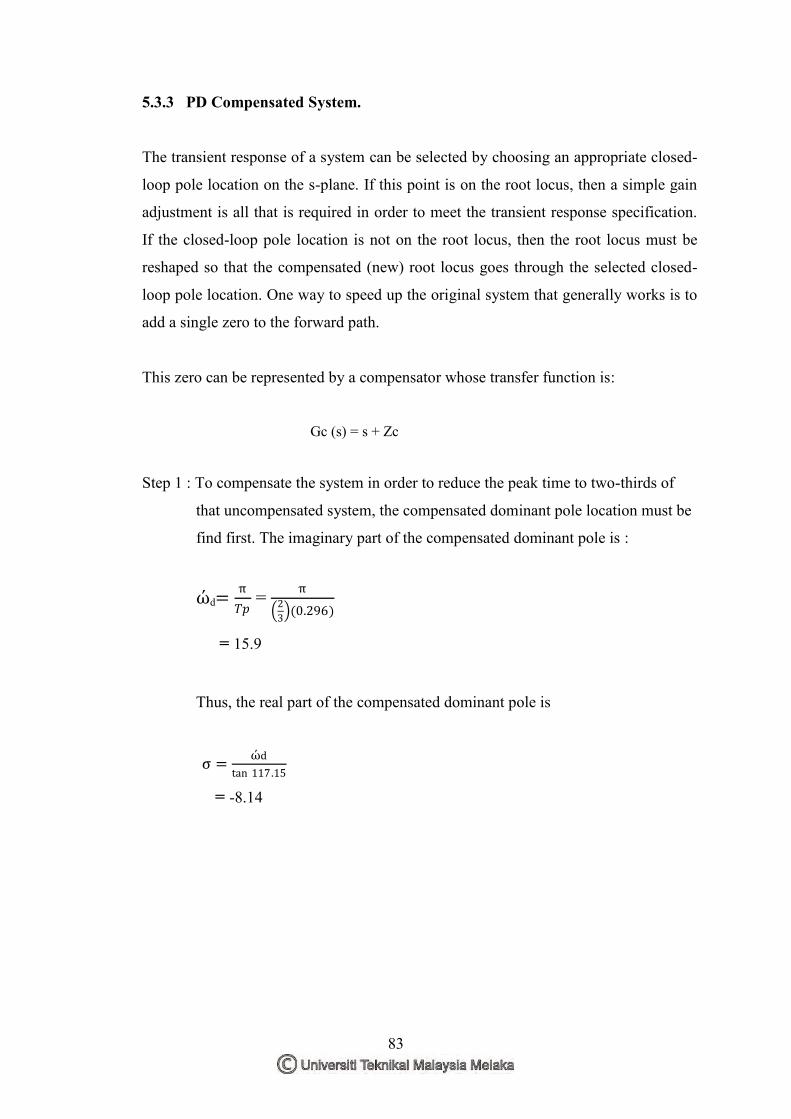
83
5.3.3 PD Compensated System.
The transient response of a system can be selected by choosing an appropriate closed-
loop pole location on the s-plane. If this point is on the root locus, then a simple gain
adjustment is all that is required in order to meet the transient response specification.
If the closed-loop pole location is not on the root locus, then the root locus must be
reshaped so that the compensated (new) root locus goes through the selected closed-
loop pole location. One way to speed up the original system that generally works is to
add a single zero to the forward path.
This zero can be represented by a compensator whose transfer function is:
Gc (s) = s + Zc
Step 1 : To compensate the system in order to reduce the peak time to two-thirds of
that uncompensated system, the compensated dominant pole location must be
find first. The imaginary part of the compensated dominant pole is :
ώd=π
𝑇𝑝 = π
2
3 (0.296)
= 15.9
Thus, the real part of the compensated dominant pole is
σ =ώd
tan 117.15
= -8.14
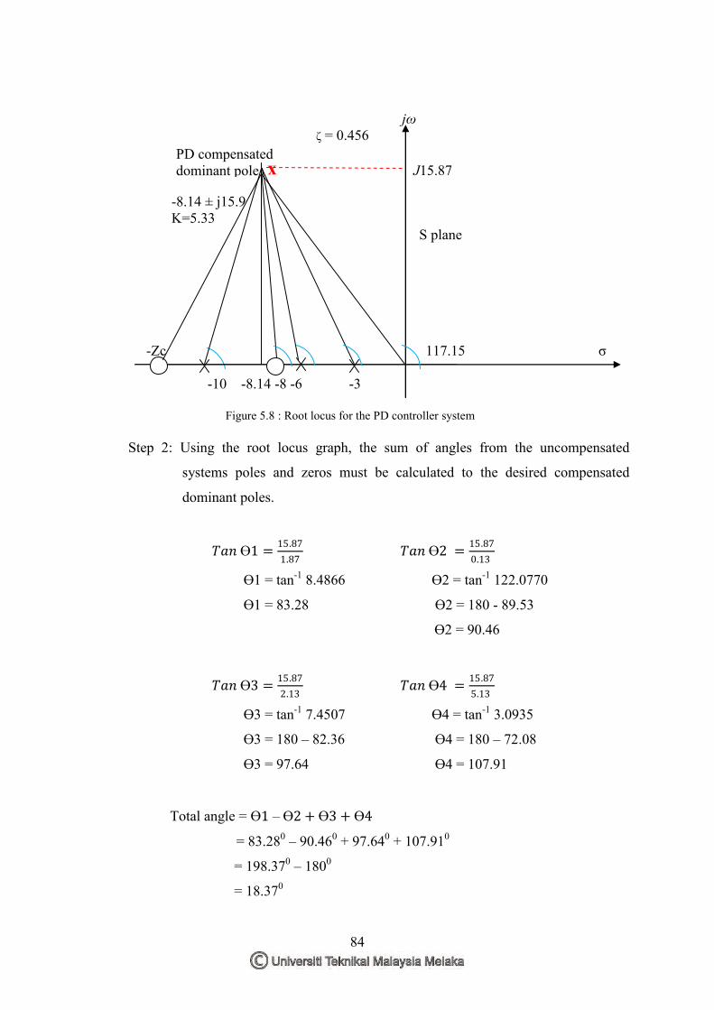
84
jω ζ = 0.456 -8.14 ± j15.9 K=5.33 S plane -Zc 117.15 σ -10 -8.14 -8 -6 -3 Figure 5.8 : Root locus for the PD controller system
Step 2: Using the root locus graph, the sum of angles from the uncompensated
systems poles and zeros must be calculated to the desired compensated
dominant poles.
𝑇𝑎𝑛 Ө1 =15.87
1.87 𝑇𝑎𝑛 Ө2 =
15.87
0.13
Ө1 = tan-1 8.4866 Ө2 = tan-1 122.0770
Ө1 = 83.28 Ө2 = 180 - 89.53
Ө2 = 90.46
𝑇𝑎𝑛 Ө3 =15.87
2.13 𝑇𝑎𝑛 Ө4 =
15.87
5.13
Ө3 = tan-1 7.4507 Ө4 = tan-1 3.0935
Ө3 = 180 – 82.36 Ө4 = 180 – 72.08
Ө3 = 97.64 Ө4 = 107.91
Total angle = Ө1 – Ө2 + Ө3 + Ө4
= 83.280 – 90.460 + 97.640 + 107.910
= 198.370 – 1800
= 18.370
x PD compensated dominant pole J15.87
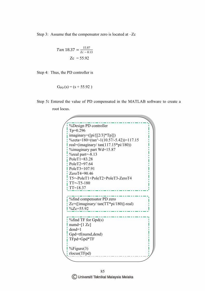
85
Step 3: Assume that the compensator zero is located at –Zc
𝑇𝑎𝑛 18.37 =15.87
𝑍𝑐 − 8.13
Zc = 55.92
Step 4: Thus, the PD controller is
GPD (s) = (s + 55.92 )
Step 5: Entered the value of PD compensated in the MATLAB software to create a
root locus.
%Design PD controller Tp=0.296 imaginary=([pi/[[2/3]*Tp]]) %zeta=180+(tan^-1(10.57/-5.42))=117.15 real=(imaginary/ tan(117.15*pi/180)) %imaginary part Wd=15.87 %real part=-8.13 PoleT1=83.28 PoleT2=97.64 PoleT3=107.91 ZeroT4=90.46 T5=-PoleT1+PoleT2+PoleT3-ZeroT4 TT=-T5-180 TT=18.37 %find compensator PD zero Zc=([imaginary/ tan(TT*pi/180)]-real) %Zc=55.92 %find TF for Gpd(s) numd=[1 Zc] dend=1 Gpd=tf(numd,dend) TFpd=Gpd*TF %Figure(3) rlocus(TFpd)
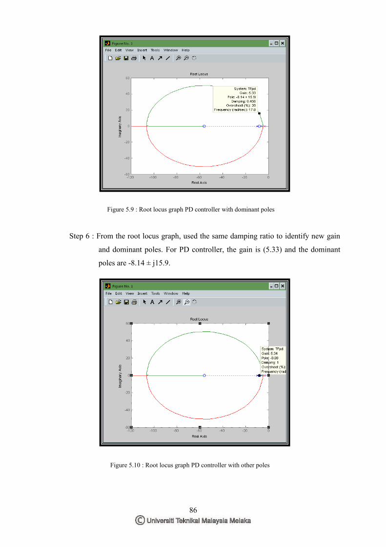
86
Figure 5.9 : Root locus graph PD controller with dominant poles
Step 6 : From the root locus graph, used the same damping ratio to identify new gain
and dominant poles. For PD controller, the gain is (5.33) and the dominant
poles are -8.14 ± j15.9.
Figure 5.10 : Root locus graph PD controller with other poles
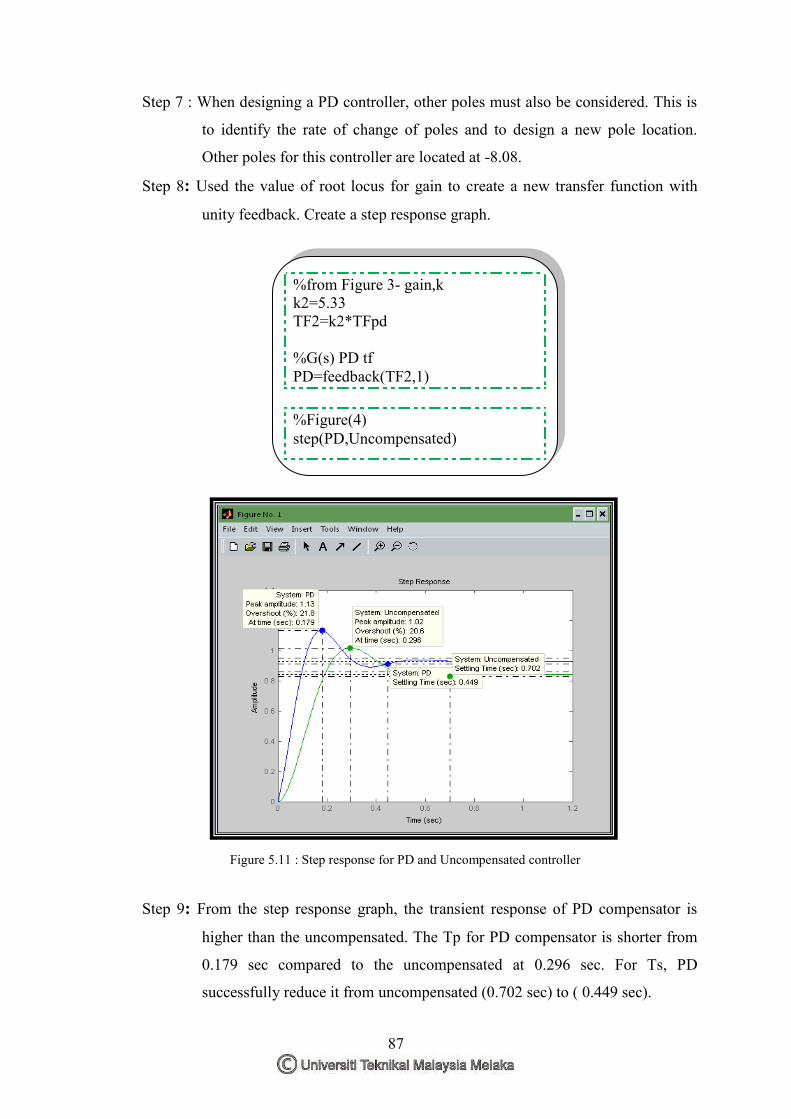
87
Step 7 : When designing a PD controller, other poles must also be considered. This is
to identify the rate of change of poles and to design a new pole location.
Other poles for this controller are located at -8.08.
Step 8: Used the value of root locus for gain to create a new transfer function with
unity feedback. Create a step response graph.
Figure 5.11 : Step response for PD and Uncompensated controller
Step 9: From the step response graph, the transient response of PD compensator is
higher than the uncompensated. The Tp for PD compensator is shorter from
0.179 sec compared to the uncompensated at 0.296 sec. For Ts, PD
successfully reduce it from uncompensated (0.702 sec) to ( 0.449 sec).
%from Figure 3- gain,k k2=5.33 TF2=k2*TFpd %G(s) PD tf PD=feedback(TF2,1) %Figure(4) step(PD,Uncompensated)
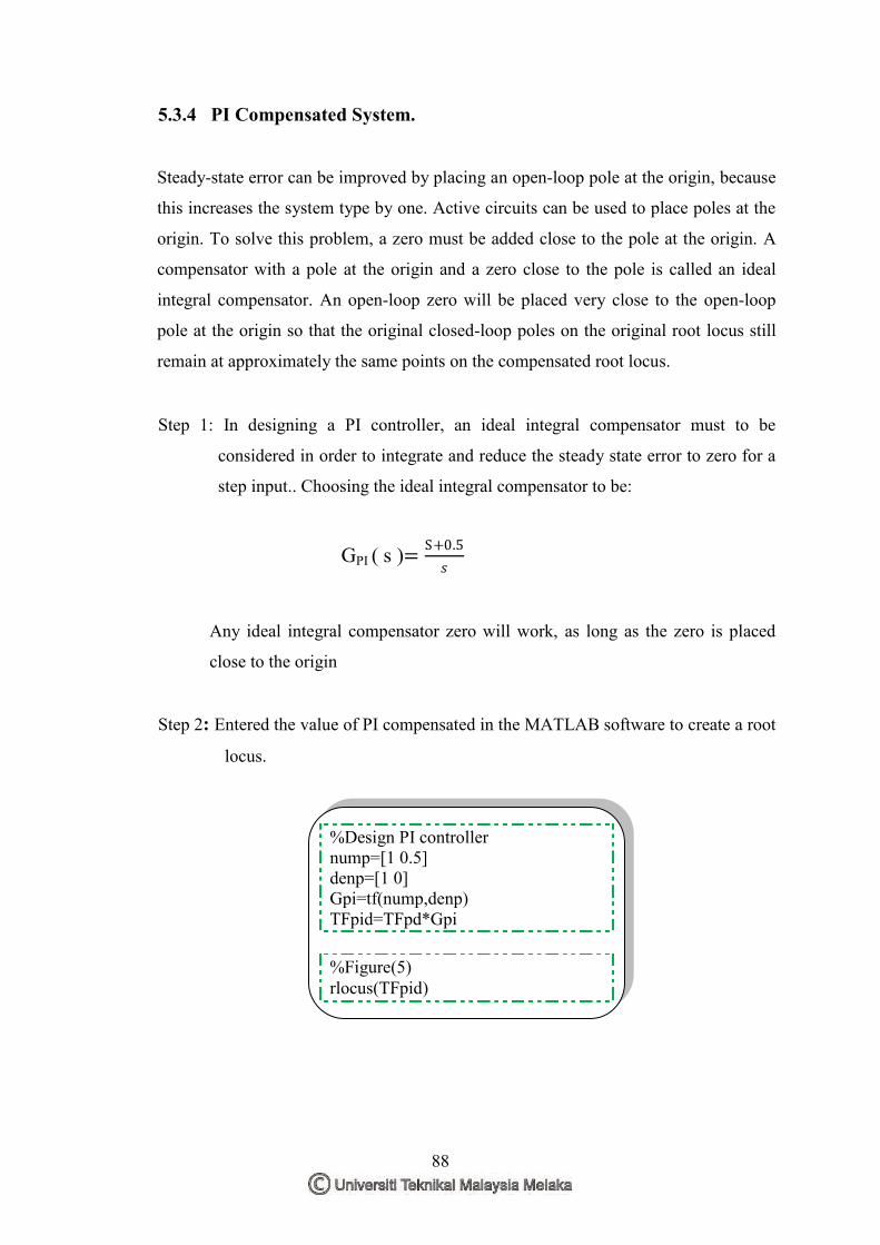
88
5.3.4 PI Compensated System.
Steady-state error can be improved by placing an open-loop pole at the origin, because
this increases the system type by one. Active circuits can be used to place poles at the
origin. To solve this problem, a zero must be added close to the pole at the origin. A
compensator with a pole at the origin and a zero close to the pole is called an ideal
integral compensator. An open-loop zero will be placed very close to the open-loop
pole at the origin so that the original closed-loop poles on the original root locus still
remain at approximately the same points on the compensated root locus.
Step 1: In designing a PI controller, an ideal integral compensator must to be
considered in order to integrate and reduce the steady state error to zero for a
step input.. Choosing the ideal integral compensator to be:
GPI ( s )= S+0.5
𝑠
Any ideal integral compensator zero will work, as long as the zero is placed
close to the origin
Step 2: Entered the value of PI compensated in the MATLAB software to create a root
locus.
%Design PI controller nump=[1 0.5] denp=[1 0] Gpi=tf(nump,denp) TFpid=TFpd*Gpi %Figure(5) rlocus(TFpid)
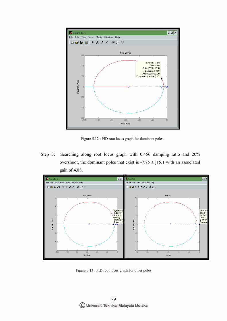
89
Figure 5.12 : PID root locus graph for dominant poles
Step 3: Searching along root locus graph with 0.456 damping ratio and 20%
overshoot, the dominant poles that exist is -7.75 ± j15.1 with an associated
gain of 4.88.
Figure 5.13 : PID root locus graph for other poles
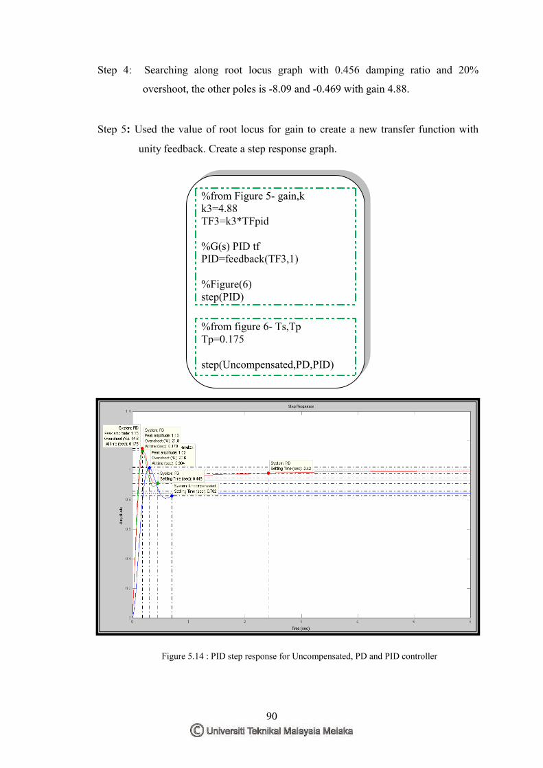
90
Step 4: Searching along root locus graph with 0.456 damping ratio and 20%
overshoot, the other poles is -8.09 and -0.469 with gain 4.88.
Step 5: Used the value of root locus for gain to create a new transfer function with
unity feedback. Create a step response graph.
Figure 5.14 : PID step response for Uncompensated, PD and PID controller
%from Figure 5- gain,k k3=4.88 TF3=k3*TFpid %G(s) PID tf PID=feedback(TF3,1) %Figure(6) step(PID) %from figure 6- Ts,Tp Tp=0.175 step(Uncompensated,PD,PID)
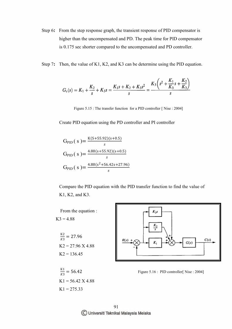
91
Step 6: From the step response graph, the transient response of PID compensator is
higher than the uncompensated and PD. The peak time for PID compensator
is 0.175 sec shorter compared to the uncompensated and PD controller.
Step 7: Then, the value of K1, K2, and K3 can be determine using the PID equation.
Figure 5.15 : The transfer function for a PID controller [ Nise : 2004]
Create PID equation using the PD controller and PI controller
GPID ( s )= K S+55.92 (s+0.5)
𝑠
GPID ( s )= 4.88 s+55.92 (s+0.5)
𝑠
GPID ( s )= 4.88 s2+56.42s+27.96
𝑠
Compare the PID equation with the PID transfer function to find the value of
K1, K2, and K3.
From the equation : K3 = 4.88
K2
𝐾3= 27.96
K2 = 27.96 X 4.88 K2 = 136.45
K1
𝐾3= 56.42 Figure 5.16 : PID controller[ Nise : 2004]
K1 = 56.42 X 4.88 K1 = 275.33
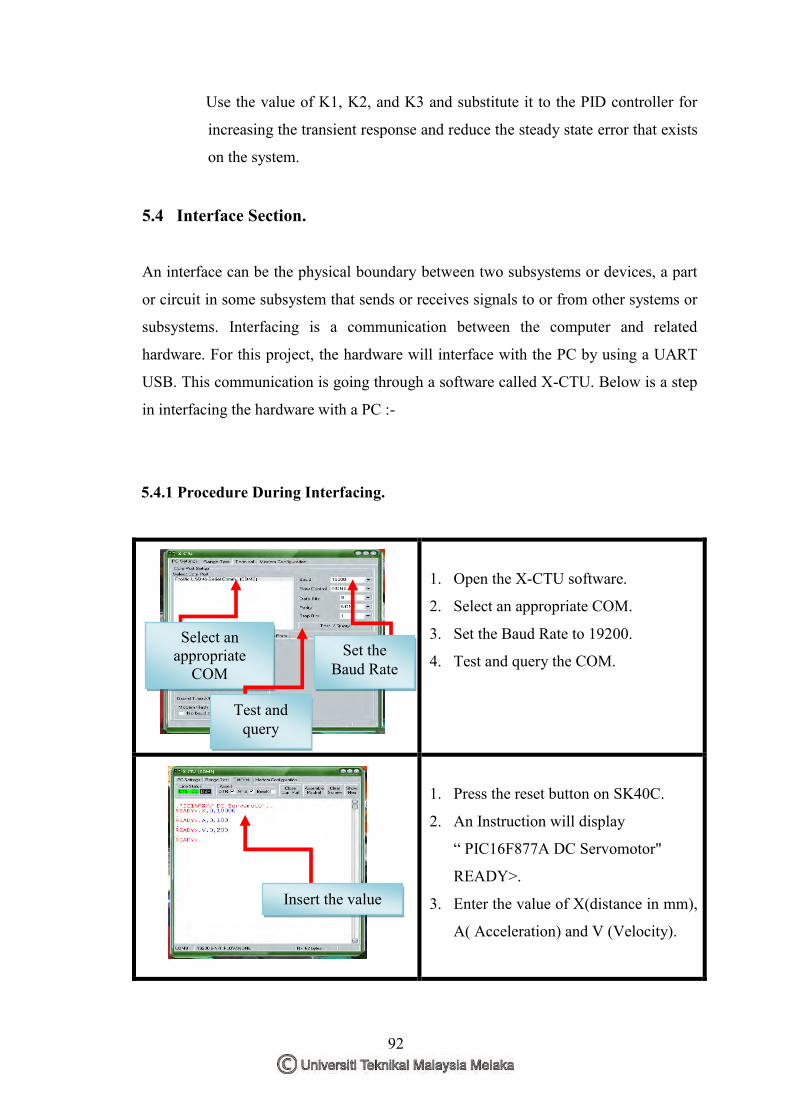
92
Use the value of K1, K2, and K3 and substitute it to the PID controller for
increasing the transient response and reduce the steady state error that exists
on the system.
5.4 Interface Section.
An interface can be the physical boundary between two subsystems or devices, a part
or circuit in some subsystem that sends or receives signals to or from other systems or
subsystems. Interfacing is a communication between the computer and related
hardware. For this project, the hardware will interface with the PC by using a UART
USB. This communication is going through a software called X-CTU. Below is a step
in interfacing the hardware with a PC :-
5.4.1 Procedure During Interfacing.
1. Open the X-CTU software.
2. Select an appropriate COM.
3. Set the Baud Rate to 19200.
4. Test and query the COM.
1. Press the reset button on SK40C.
2. An Instruction will display
“ PIC16F877A DC Servomotor"
READY>.
3. Enter the value of X(distance in mm),
A( Acceleration) and V (Velocity).
Select an appropriate
COM
Insert the value
Set the Baud Rate
Test and query
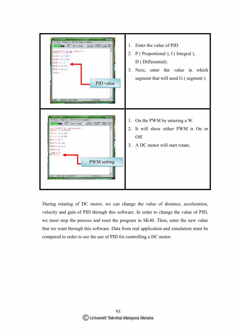
93
During rotating of DC motor, we can change the value of distance, acceleration,
velocity and gain of PID through this software. In order to change the value of PID,
we must stop the process and reset the program in SK40. Then, enter the new value
that we want through this software. Data from real application and simulation must be
compared in order to see the use of PID for controlling a DC motor.
1. Enter the value of PID.
2. P ( Proportional ), I ( Integral ),
D ( Differential).
3. Next, enter the value in which
segment that will used G ( segment ).
1. On the PWM by entering a W.
2. It will show either PWM is On or
Off.
3. A DC motor will start rotate.
PID value
PWM setting
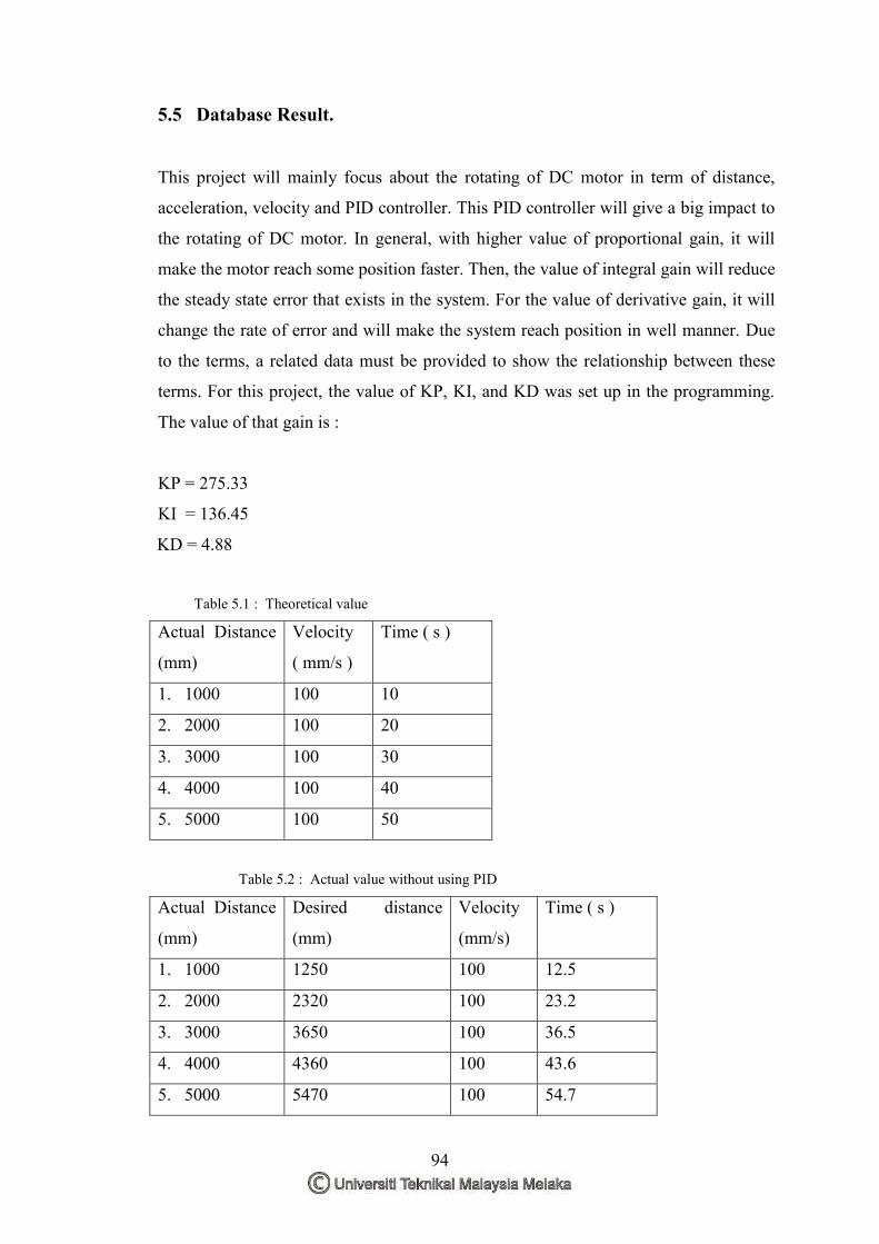
94
5.5 Database Result.
This project will mainly focus about the rotating of DC motor in term of distance,
acceleration, velocity and PID controller. This PID controller will give a big impact to
the rotating of DC motor. In general, with higher value of proportional gain, it will
make the motor reach some position faster. Then, the value of integral gain will reduce
the steady state error that exists in the system. For the value of derivative gain, it will
change the rate of error and will make the system reach position in well manner. Due
to the terms, a related data must be provided to show the relationship between these
terms. For this project, the value of KP, KI, and KD was set up in the programming.
The value of that gain is :
KP = 275.33
KI = 136.45
KD = 4.88
Table 5.1 : Theoretical value
Actual Distance
(mm)
Velocity
( mm/s )
Time ( s )
1. 1000 100 10
2. 2000 100 20
3. 3000 100 30
4. 4000 100 40
5. 5000 100 50
Table 5.2 : Actual value without using PID
Actual Distance
(mm)
Desired distance
(mm)
Velocity
(mm/s)
Time ( s )
1. 1000 1250 100 12.5
2. 2000 2320 100 23.2
3. 3000 3650 100 36.5
4. 4000 4360 100 43.6
5. 5000 5470 100 54.7

95
0
1000
2000
3000
4000
5000
6000
10 20 30 40 50
Dis
tan
ce (
mm
)
Time ( s )
Graph Distance (m ) versus Time (s
Theorytical value
Actual value without PID
Figure 5.17 : Graph for Theorytical value and Actual value without PID
From the graph, the actual value without PID from rotation of DC motor is too far
away from theoretical value. This is could be happen when the motor difficult to
achieved exact distance entered by the user. When motor travel along a path of
distance, speed, distance and time is the important element has to be considered.
Without having an accurate value of that item, the DC motor will not give an accurate
and reliable value. To prevent from this thing happen, a PID controller was
introduced. Then, the flow of the process continued with PID configuration. This is
done by entering the value of P, I , and D in X-CTU software. The command for
entering this value as shown as follow:
X,0,1000 // Entering the distance value in ( mm )
V,0,100 // Entering the velocity value in ( mm/s )
P,1 // Entering the Proportional value
D,1 // Entering the Differential value
G,0,0 // Entering the Segment value
W // PWM ON
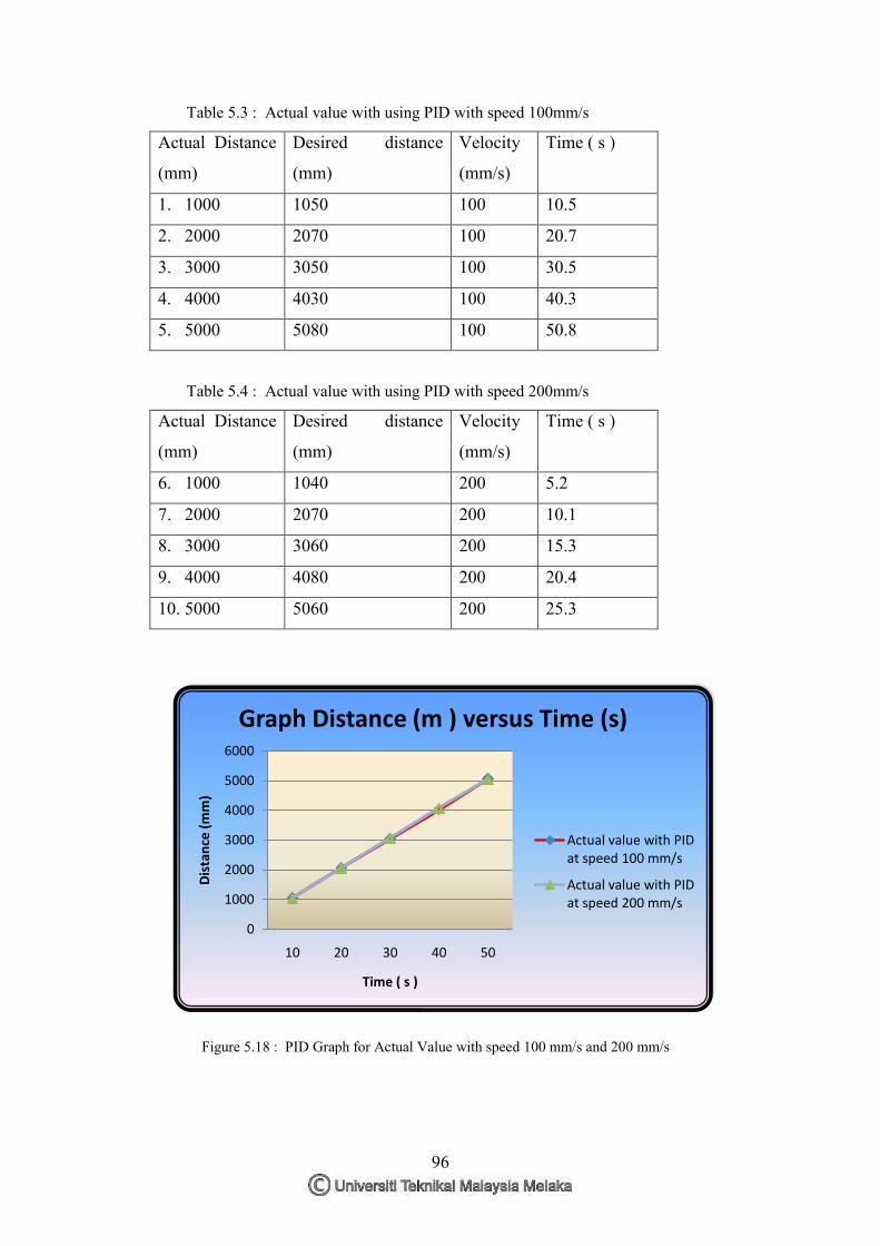
96
0
1000
2000
3000
4000
5000
6000
10 20 30 40 50
Dis
tan
ce (
mm
)
Time ( s )
Graph Distance (m ) versus Time (s)
Actual value with PID at speed 100 mm/s
Actual value with PID at speed 200 mm/s
Table 5.3 : Actual value with using PID with speed 100mm/s
Actual Distance
(mm)
Desired distance
(mm)
Velocity
(mm/s)
Time ( s )
1. 1000 1050 100 10.5
2. 2000 2070 100 20.7
3. 3000 3050 100 30.5
4. 4000 4030 100 40.3
5. 5000 5080 100 50.8
Table 5.4 : Actual value with using PID with speed 200mm/s
Actual Distance
(mm)
Desired distance
(mm)
Velocity
(mm/s)
Time ( s )
6. 1000 1040 200 5.2
7. 2000 2070 200 10.1
8. 3000 3060 200 15.3
9. 4000 4080 200 20.4
10. 5000 5060 200 25.3
Figure 5.18 : PID Graph for Actual Value with speed 100 mm/s and 200 mm/s
97
From this project, several experiments were conducted to get a data. From the graph,
we can see that a PID controller gives a good impact to the response of the DC motor.
The response for graph actual value with speed of 100 mm/s is almost nearest to the
response graph actual value with speed of 200 mm/s. These things happen as the PID
controller execute its role to increase the transient response and reduce steady state
errors that exist in this system. By increasing the transient response of the system, the
rotation of DC motor achieved the distance in well manner and reliable. For steady
state error, this PID controller will integrate the error by reducing the range of error
and make it zero through differential section.
5.6 Conclusion and Finding.
Based on the finding for this project, several objectives were not achieved for this
project. The problem is the real application does not give the exact value compared to
the simulation using proteus software. This problem occurres because of the several
elements such as the value of PID controller and programming section. For designing
a PID controller, a transfer function represent the DC motor is a standard from the
references book. This project used a Pittman DC servomotor that having an encoder
that can be able performs of wide variety of operation. Another problem exist is
communication between hardware and computer using serial port. A computer not
received an accurate signal from the hardware to perform a given task.
In the programming section, it is hard to define the related command that being used to
communicate between hardware and computer. Other command like register, timer,
interrupt and others should be match with the hardware to make it easier while
communicate process. Other related problem exist in this project is the embedded
circuit is quite difficult to design and developed. The complex of the circuit will
trigger a lack of transmission signal to the other component to perform an operation. It
too hard to find if any line break along of PCB layout during transmission signal.
Some improvement should be made and will discuss more in the next chapter.
98
CHAPTER 6 CONCLUSION AND RECOMMENDATION
6.0 Background
In this chapter, the conclusion from the entire project will be include with the
recommendation and also the suggestion for future or nowadays.
6.1 Conclusion
This project explored the way for controlling a DC motor using a control system
element which is PID. Nowadays, most of the system have their weaknesses due to
some disturbances such as noise, lack of transient response and large of steady state
error. To overcome this problem, a PID controller was introduced. This PID controller
increase the transient response of the system instead of reducing of steady state error
that exist on that system. Beside that, the project is study the method for controlling a
DC motor either use a PWM or H- Bridge technique. In general, this project will
mainly focus on the method for controlling a DC motor, the element should be added
to make the system operate in less error and the communication between the hardware
and computer. Overall, this project succesfully fulfill all the objectives requirement
which is to design and develop the embedded system, to study the PID controller, to
design a PID controller and lastly to get an exact position during the rotation of the
DC motor.The system mainly provides an efficient method for surveillance purpose
and is aimed to be highly beneficial.
99
6.2 Recommendation and Future Work.
The performance for this embedded system is not meet the full requirement in
objective. For future work, some recommendation has been listed in order to improve
the performance of this embedded system for controlling a DC motor.
1. Find an exact transfer function for PID controller.
To get an accurate value of the gain for Kp, Ki, and KD, an exact transfer function
are needed in order to generate a smooth and accurate step response for PID
controller. For this project, there two transfer function are highly needed which is
for the DC motor and for the plant. Then, the unity feedback transfer function for
this project should be identify also which is the encoder.
2. Serial port communication.
During communication between hardware and computer, several problem occured
such as loss in receiving the data and difficult to transmit the data. Formerly, this
project use a RS 232 cable during interface section. By using this RS 232 cable, no
data was successfully sent to the hardware. Then, from RS 232 cable, the interface
section changed to use bluetooh serial communication. Bluetooth serial
communication has their weaknesses such as can transmit or receive data on
certain distance only. To overcome this problem, USB USART was introduced
that consist a TX ( transmit ) and RX ( receive ) terminal in order to transmit or
received the data.
3. Software improvement
For interface testing, hyper terminal was used to communicate between computer
and software, but small problem exist during communication such as didn’t able to
sent the data to the hardware. To overcome this problem, one software has been
introduced which is X-CTU that consit a comm port, baud, flow control, data bits
and parity for specific task. By using this X-CTU software, communication was
succesfully done between hardware and computer.
100
4. Vary the speed with PID controller.
This project will mainly focus on the desired distance only. To get an accurate
distance during rotation of DC motor with same speed, a PID controller was
introduced. For future work, this system need to redesign with adding an element
that can control the speed of DC motor rotation.
5. Mathematical modeling of motor response
Mathematical model can be obtained from the graph of motor speed response.
Then, from the mathematical model, it can be simulated using software such as
MATLAB to improved motor speed response by using controller packages such as
PID controller, Fuzzy Logic Controller and others. Besides, it will reduce the total
hardware complexity and cost at the same time.
101
REFERENCES
Aidan O’Dwyer (2009). “ Handbook of PI and PID controllers Tuning Rules”. London :
Imperial College Press, pp. 80-93
Ang, K.H., Chong, G.C.Y., and Li, Y. (2005). “PID control system analysis, design, and
technology”,IEEE Trans Control Systems Tech.pp.559-576. http://eprints.gla.ac.uk/3817/
(Accessed: 19 August 2010).
Antonio Visioli (2006). “ Practical PID control”. London : Springer, pp 1-15
Austin Hughes (1997). “ Electric motor and drives”. England : Newness, pp 84-90
Bennett, Stuart (1993). “A history of control engineering”. London : IET. pp 48
Bennett, Stuart (June 1986). “A history of control engineering”.IET. pp. 142–148
Dr. Steve C. Hsiung, (2007). “ The Use of PIC Microcontrollers in Multiple DC Motors
Control Applications”. Pp. 6-8
Gourab Sen Gupta,(2005). “A Project Based Approach to Teach Mixed-Signal Embedded
Microcontroller for DC Motor Control”.pp. 5-6
Greg Osborn. “Embedded microcontrollers and processor design”. New Jersey: Prentice
Hall pp. 4-20
Hongfu Zhou, (2008). “DC Servo Motor PID Control in Mobile Robots with Embedded
DSP”. pp. 1-4
102
Omar Jones (2010). “Design And Development Of An Embedded Dc Motor Controller
Using A Pid Algorithm”. pp. 5-7
Paul Horowitz and Winfield Hil (1989). ”The Art of Electronics Second Edition”.
Cambridge University Press, Cambridge M: pp 723-726
Shibu KV (2009). “Intoduction To Embedded Systems.” New York: McGraw Hill, pp.4-
15
Stephen Bowling, (2000). “DC Servomotor Application”. pp. 1-7
S. Vazquez, (2008). “Controller Design for a Single-Phase Two-Cell Multilevel Cascade
H-Bridge Converter”. Pp 2342
Tanmay Pal, Chandra Shekhar and Himanshu Dutt Sharma, (2009). “Design and
Development of Embedded System on ARM for On-line Characterization of DC
Motor”.pp. 502-503
Todd D. Morton. “Embedded Microcontrollers.” New Jersey: Prentice Hall, pp. 1-34
Vladimir Gurevich (2008). “ Electronic Devices on Discrete Components for Industrial
and Power Engineering”. London - New York : CRC Press, pp.418
W Bolton (1992). “ Control Engineering”. England : Longman, pp 233-237
Y. S. E. Ali, S. B. M. Noor, S. M. Uashi and M. K Hassan, (2003). “Microcontroller
Performance for DC Motor Speed Control System”. Pp. 2-5
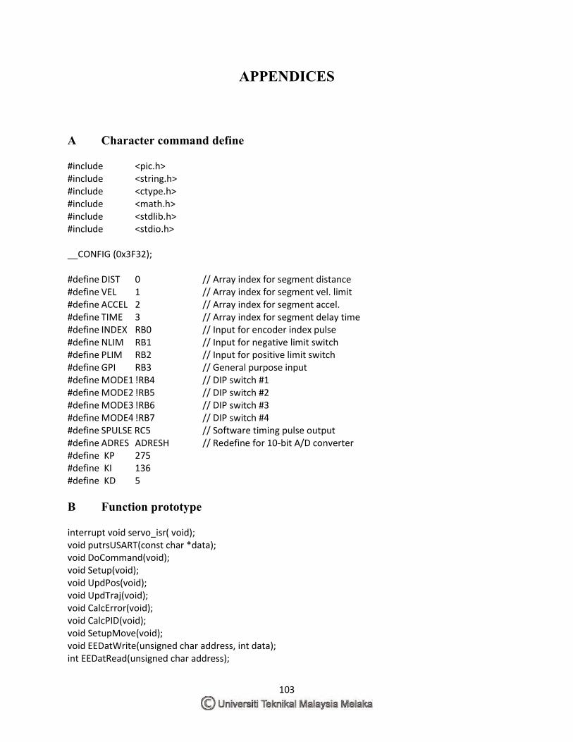
103
APPENDICES
A Character command define #include <pic.h> #include <string.h> #include <ctype.h> #include <math.h> #include <stdlib.h> #include <stdio.h> __CONFIG (0x3F32); #define DIST 0 // Array index for segment distance #define VEL 1 // Array index for segment vel. limit #define ACCEL 2 // Array index for segment accel. #define TIME 3 // Array index for segment delay time #define INDEX RB0 // Input for encoder index pulse #define NLIM RB1 // Input for negative limit switch #define PLIM RB2 // Input for positive limit switch #define GPI RB3 // General purpose input #define MODE1 !RB4 // DIP switch #1 #define MODE2 !RB5 // DIP switch #2 #define MODE3 !RB6 // DIP switch #3 #define MODE4 !RB7 // DIP switch #4 #define SPULSE RC5 // Software timing pulse output #define ADRES ADRESH // Redefine for 10-bit A/D converter #define KP 275 #define KI 136 #define KD 5
B Function prototype interrupt void servo_isr( void); void putrsUSART(const char *data); void DoCommand(void); void Setup(void); void UpdPos(void); void UpdTraj(void); void CalcError(void); void CalcPID(void); void SetupMove(void); void EEDatWrite(unsigned char address, int data); int EEDatRead(unsigned char address);
104
C Servo calculation interrupt void servo_isr(void) { SPULSE = 1; // Toggle output pin for ISR code UpdTraj(); // Get new commanded position UpdPos(); // Get new measured position CalcError(); // Calculate new position error CalcPID(); TMR2IF = 0; // Clear Timer2 Interrupt Flag. SPULSE = 0; // Toggle output pin for ISR code } // timing
D Motion calculation void UpdTraj(void) { if(stat.motion && !stat.saturated) { if(!stat.phase) // If in the first half of the move. { if(velact.ui[1] < vlim) // If still below the velocity limit velact.ul += accel.ul; // Accelerate else // If velocity limit has been reached, flatcount++; // increment flatcount. temp.ul = velact.ul; // Put velocity value into temp if(velact.ui[0] == 0x8000) { if(!(velact.ub[2] & 0x01)) temp.ui[1]++; else; } else if(velact.ui[0] > 0x8000) temp.ui[1]++; else; phase1dist.ul -= (unsigned long)temp.ui[1]; if(stat.neg_move) position -= (unsigned long)temp.ui[1]; else position += (unsigned long)temp.ui[1]; }
105
E Position setup void UpdPos(void) { mvelocity = DnCount; // Get old DnCount value temp.b[0] = TMR1L; // Read Timer1 temp.b[1] = TMR1H; if(TMR1L < temp.b[0]) // If a rollover occurred, read { // Timer1 again. temp.b[0] = TMR1L; temp.b[1] = TMR1H; } DnCount = temp.i[0]; // Store timer value in DnCount mvelocity -= DnCount; // Subtract new value from tempch = -UpCount; // Put old UpCount value in UpCount = TMR0; // Read Timer0 tempch += UpCount; if(tempch > 0) mvelocity += (int)tempch; else mvelocity -= (int)(tempch); mposition += (long)(mvelocity << 8); // Update measured position }
F Error calculation void CalcError(void) { u0.l = mposition - position; // Get error u0.b[0] = u0.b[1]; u0.b[1] = u0.b[2]; // shift to the right to discard u0.b[2] = u0.b[3]; // lower 8 bits. if (u0.b[2] & 0x80) // If error is negative. { u0.b[3] = 0xff; // Sign-extend to 32 bits. if((u0.i[1] != 0xffff) || !(u0.b[1] & 0x80)) { u0.ui[1] = 0xffff; // Limit error to 16-bits. u0.ui[0] = 0x8000; } else; } else // If error is positive. { u0.b[3] = 0x00; if((u0.i[1] != 0x0000) || (u0.b[1] & 0x80))
106
{ u0.ui[1] = 0x0000; // Limit error to 16-bits. u0.ui[0] = 0x7fff; } else; } }
G PID calculation
void CalcPID(void) { ypid.l = (long)u0.i[0]*(long)kp; // If proportional gain is not 0, // calculate proportional term. if(!stat.saturated) // If output is not saturated, integral += u0.i[0]; // add present error to integral // value. if(ki) // If integral value is not 0, ypid.l += (long)integral*(long)ki; // calculate integral term. if(kd) // If differential term is not 0, ypid.l += (long)mvelocity*(long)kd; // calculate differential term. if(ypid.b[3] & 0x80) // If PID result is negative { if((ypid.b[3] < 0xff) || !(ypid.b[2] & 0x80)) { ypid.ui[1] = 0xff80; // Limit result to 24-bit value ypid.ui[0] = 0x0000; } else; } else // If PID result is positive { if(ypid.b[3] || (ypid.b[2] > 0x7f)) { ypid.ui[1] = 0x007f; // Limit result to 24-bit value ypid.ui[0] = 0xffff; } else; } ypid.b[0] = ypid.b[1]; // Shift PID result right to ypid.b[1] = ypid.b[2]; // get upper 16 bits. stat.saturated = 0; // Clear saturation flag and see if(ypid.i[0] > 500) // if present duty cycle output { // exceeds limits.

107
ypid.i[0] = 500; stat.saturated = 1; } if(ypid.i[0] < -500) { ypid.i[0] = -500; stat.saturated = 1; }
H Register define void Setup(void) { firstseg = 0; // Initialize motion segment lastseg = 0; // variables segnum = 0; parameter = 0; // Motion segment parameter# i = 0; // Receive buffer index comcount = 0; // Input command index udata = 0; // Holds USART received data stat.phase = 0; // Initialize flags and variables stat.saturated = 0; // used for servo calculations. stat.motion = 0; stat.run = 0; stat.loop = 0; stat.neg_move = 0; dtime = 0; integral = 0; vlim = 0; velcom = 0; mvelocity = 0; DnCount = 0; UpCount = 0; temp.l = 0; accel.l = 0; u0.l = 0; ypid.l = 0; velact.l = 0; phase1dist.l = 0; position = 0; mposition = position; fposition = position; flatcount = 0; memset(inpbuf,0,8); // clear the input buffer udata = RCREG; udata = RCREG; RCREG = 0; udata = 0;
108
SPBRG = 15; // 19200 baud @ 20MHz BRGH = 1; //TXEN = 1; //CREN = 1; //SPEN = 1; TXSTA = 0x20; // setup USART transmit RCSTA = 0x90; // setup USART receive SSPADD = 49; // Setup MSSP for master I2C SSPSTAT = 0; // 100Khz @ 20MHz SSPCON2 = 0; SSPCON = 0x28; PR2 = 0xff; // Setup Timer2 and CCP1 for T2CON = 0x4c; // 19.53 Khz PWM @ 20MHz CCPR1L = 0x7f; // 50% initial duty cycle CCP1CON = 0x0f; TMR2IF = 0; TMR2IE = 1; // Enable Timer2 interrupts TMR1H = 0; TMR1L = 0; T1CON = 0x07; // Enable Timer1, ext. sync. clock TMR0 = 0; OPTION = 0x6f; // Enable Timer0 ADCON1 = 0x04; // Setup A/D converter ADCON0 = 0x81; PORTC = 0; // Clear PORTC PORTD = 0; // Clear PORTD PORTE = 0x00; // Clear PORTE TRISC = 0xdb; TRISD = 0; // PORTD all outputs TRISE = 0; // PORTE all outputs
I Main program
main() { Setup(); putrsUSART("\r\nPIC16F877 DC Servomotor"); putrsUSART(ready); for(segnum=0;segnum < 12;segnum++) // Reads profile data into RAM for { for(parameter=0;parameter < 4;parameter++) { eeadr = (segnum << 3) + (parameter << 1); segment1[segnum][parameter] = EEDatRead(eeadr); } }
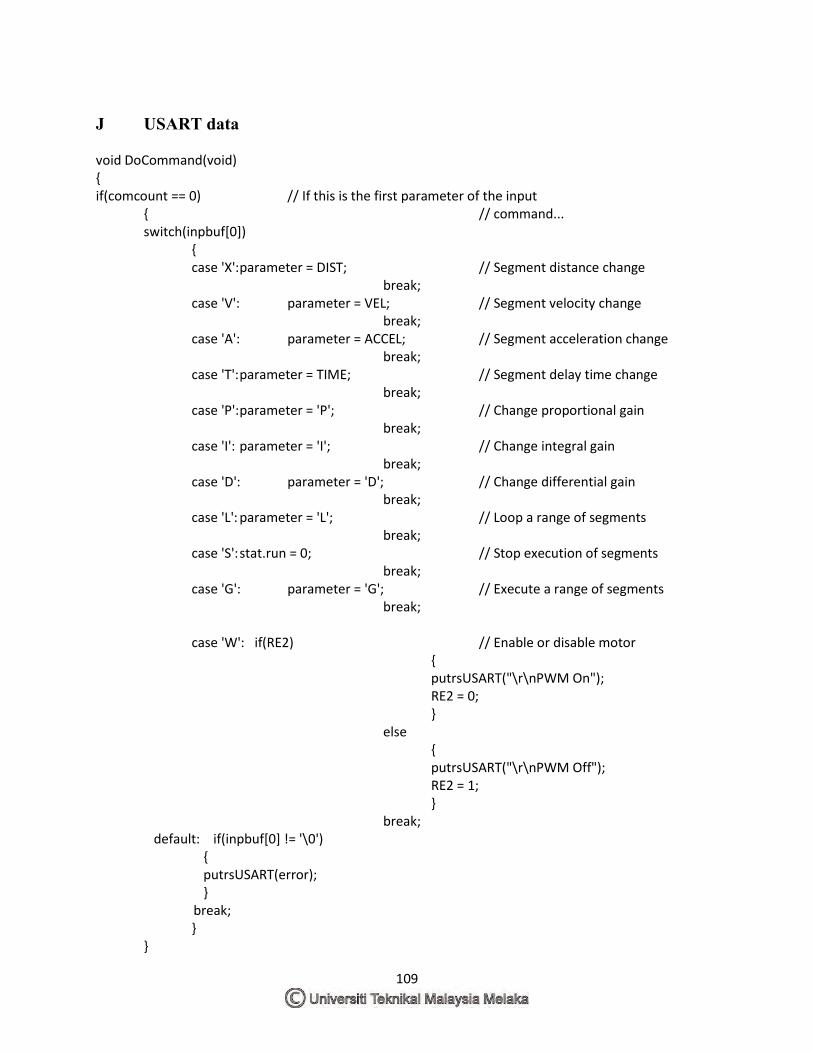
109
J USART data void DoCommand(void) { if(comcount == 0) // If this is the first parameter of the input { // command... switch(inpbuf[0]) { case 'X': parameter = DIST; // Segment distance change break; case 'V': parameter = VEL; // Segment velocity change break; case 'A': parameter = ACCEL; // Segment acceleration change break; case 'T': parameter = TIME; // Segment delay time change break; case 'P': parameter = 'P'; // Change proportional gain break; case 'I': parameter = 'I'; // Change integral gain break; case 'D': parameter = 'D'; // Change differential gain break; case 'L': parameter = 'L'; // Loop a range of segments break; case 'S': stat.run = 0; // Stop execution of segments break; case 'G': parameter = 'G'; // Execute a range of segments break; case 'W': if(RE2) // Enable or disable motor { putrsUSART("\r\nPWM On"); RE2 = 0; } else { putrsUSART("\r\nPWM Off"); RE2 = 1; } break; default: if(inpbuf[0] != '\0') { putrsUSART(error); } break; } }


