University of Tennessee, Knoxville University of Tennessee, Knoxville TRACE: Tennessee Research and Creative TRACE: Tennessee Research and Creative Exchange Exchange Chancellor’s Honors Program Projects Supervised Undergraduate Student Research and Creative Work 5-2014 Design and Economic Analysis of a Geothermal Vertical Coupled Design and Economic Analysis of a Geothermal Vertical Coupled Heat Pump System for the University of Tennessee, Knoxville Heat Pump System for the University of Tennessee, Knoxville Campus Campus Joseph W. Birchfield IV University of Tennessee-Knoxville, jbirchfi@utk.edu Will Kester University of Tennessee-Knoxville, [email protected]Jason Cho University of Tennessee-Knoxville, [email protected]Follow this and additional works at: https://trace.tennessee.edu/utk_chanhonoproj Part of the Geotechnical Engineering Commons, Heat Transfer, Combustion Commons, Other Chemical Engineering Commons, and the Thermodynamics Commons Recommended Citation Recommended Citation Birchfield, Joseph W. IV; Kester, Will; and Cho, Jason, "Design and Economic Analysis of a Geothermal Vertical Coupled Heat Pump System for the University of Tennessee, Knoxville Campus" (2014). Chancellor’s Honors Program Projects. https://trace.tennessee.edu/utk_chanhonoproj/1736 This Dissertation/Thesis is brought to you for free and open access by the Supervised Undergraduate Student Research and Creative Work at TRACE: Tennessee Research and Creative Exchange. It has been accepted for inclusion in Chancellor’s Honors Program Projects by an authorized administrator of TRACE: Tennessee Research and Creative Exchange. For more information, please contact [email protected].
Transcript
University of Tennessee, Knoxville University of Tennessee, Knoxville
TRACE: Tennessee Research and Creative TRACE: Tennessee Research and Creative
Exchange Exchange
Chancellor’s Honors Program Projects Supervised Undergraduate Student Research and Creative Work
5-2014
Design and Economic Analysis of a Geothermal Vertical Coupled Design and Economic Analysis of a Geothermal Vertical Coupled
Heat Pump System for the University of Tennessee, Knoxville Heat Pump System for the University of Tennessee, Knoxville
Campus Campus
Joseph W. Birchfield IV University of Tennessee-Knoxville, [email protected]
Follow this and additional works at: https://trace.tennessee.edu/utk_chanhonoproj
Part of the Geotechnical Engineering Commons, Heat Transfer, Combustion Commons, Other
Chemical Engineering Commons, and the Thermodynamics Commons
Recommended Citation Recommended Citation Birchfield, Joseph W. IV; Kester, Will; and Cho, Jason, "Design and Economic Analysis of a Geothermal Vertical Coupled Heat Pump System for the University of Tennessee, Knoxville Campus" (2014). Chancellor’s Honors Program Projects. https://trace.tennessee.edu/utk_chanhonoproj/1736
This Dissertation/Thesis is brought to you for free and open access by the Supervised Undergraduate Student Research and Creative Work at TRACE: Tennessee Research and Creative Exchange. It has been accepted for inclusion in Chancellor’s Honors Program Projects by an authorized administrator of TRACE: Tennessee Research and Creative Exchange. For more information, please contact [email protected].
Design and Economic Analysis of a Geothermal Vertical Coupled Heat Pump System for the University of
Tennessee Campus
Joey Birchfield
Jason Cho
Will Kester
Table of Contents
1. Introduction
2. Synthesis Information for Processes
3. Method of Approach
4. Results
5. Capital Cost Estimates
6. Discussion of Results
7. Conclusions
8. Recommendations
9. References
10. Appendices
1. Introduction
The purpose of this report is to document a study-level design and economic analysis of a vertical
ground coupled heat system (VGCHPS) for the University of Tennessee campus. Commercial geothermal
heat pump systems are being developed to provide clean energy and reduce overall heating and cooling
costs. VGCHP’s are closed loop system’s which use a reversible vapor compression cycle linked to an
underground heat exchanger. Both the water to air and the water to water heat pumps utilize a circulating
water-antifreeze solution. The solution circulates through an underground piping network and through a
liquid-to-refrigerant coil. Fluid to be heated or cooled is circulated through a fluid-to-refrigerant coil and
is transported to the point of utilization. VGCHPS’s are normally constructed using two polyethylene
tubes in the borehole. The polyethylene tubes are connected at bottom of the bore resulting in a closed U-
tube shape. Vertical tube sizes are usually in the range from ¾ to 1.5 inches nominal diameter. Depending
on drilling conditions and underground soil properties the vertical bore depths can range from 50 to 600
feet deep.
The design objectives of this project are (1) develop a flow sheet for the design process of the
VGCHP system, (2) present relevant material and energy balances, (3) provide estimates of the initial
capital cost and determine the payback period, and (4) compare the estimated economics of the VGCHPS
with the current heating and cooling costs for the University of Tennessee.The heating requirements on
campus are met by a central steam plant that uses three coal fired boilers capable of burning a total of
300,000 pounds of coal per hour and a natural gas fired turbine generator rated at 5 MW. The cooling
requirements are met by a combination of 3,000 window air conditioners ranging from 5,000 to 32,000
BTU, 500 split and package systems ranging from 1 to 60 tons, and 92 chillers ranging from 20 to 995
tons. The total cooling capacity available from all the air conditioning equipment is approximately 30,000
tons. The University of Tennessee Facilities Services has requested the study level design of a geothermal
HVAC system capable of replacing 3 chillers that provide 2400 tons cooling energy for the agriculture
portion of campus. The 2400 tons of cooling was reduced to 600 tons due to limited space on the
Agricultural Campus. This design is focused on delivering 600 tons of cooling.
This project is supported by Facility Services at the University of Tennessee (UT). This report
documents a study-level design and economic analysis of the procurement and installation of a ground-
source heat pump at UT and was prepared in Spring Semester, 2014 as fulfillment of course requirements
of CBE 488 (Sustainable Design Internship) at the University of Tennessee. Advisors for this project are
D. W. Bailey and T.E. Ledford of UT Facility Services and J.S. Watson and R. M. Counce of UT
Chemical and Biomolecular Engineering Department.
2.0 Synthesis Information for Processes
2.1 Input Information
To determine the input information for this design we used several resources including the Engineering Group Design
1, Kavanaugh and Rafferty’s Design Guide
to replace was 2400 tons but upon the completion of2400 tons with the green space available for the bore field. could be replaced, we utilized the largest open area and back calculated to determine the load that the area could withstand. The largest space on the Agricultural Ccooling. Due to the size limits of the spreadsheet, the boeach having a total cooling load of 200 tons andcalculated using this number and the Design Guide
In 2009, Engineering Services Group INC and Midstudy to determine the economic feasibility of using a VGSHP at the future University of Tennessee Sorority Village1. From this report we were able to get ground property information including thermal conductivity, thermal diffusivity, and local ground temperature. the Engineering Services Group studyValley Authority from their geothermal test well data
We were also able to obtain recommended values for design variables such as the equivalent diameter of the bore and the spacing between adjacent bores. input information was determined using the Kavanaugh and Rafferty
The remaining borehole specificationquarter inch high density polyethylene pipe. To determine the type of grout to use and the grout properties, GeoPro Inc., who specialrecommended type of grout along with its properties
Figure 2.1 shows the hierarchal structure of the spreadsheet that will be used to calculate the depth of each borehole. For a single borehole, the by the building, soil properties, heating or cooling fluid properties, heat pump outlet temperature, average fluid temperature in the borehole, and the characteristics of the borehole, such as the radiborehole. For a borefield, all of the information required for a single borehole is included as well as the distance between boreholes, number of boreholes, and the aspect ratio of the borefield.
on for Processes
To determine the input information for this design we used several resources including the , Kavanaugh and Rafferty’s Design Guide
2. The requested amount of cooling
upon the completion of calculations, it was deemed impossible to replace e available for the bore field. To determine the maximum cooling load that the largest open area and back calculated to determine the load that the area
gest space on the Agricultural Campus was able to replace a total of 60. Due to the size limits of the spreadsheet, the borehole field was divided into three equal parts
each having a total cooling load of 200 tons and the hourly, monthly, and yearly ground loads were using this number and the Design Guide
2.
In 2009, Engineering Services Group INC and Mid-State Construction completed an engineering study to determine the economic feasibility of using a VGSHP at the future University of Tennessee
. From this report we were able to get ground property information including thermal al diffusivity, and local ground temperature. To verify that the information provided in
study we compared their values with values reported by the Tennessee from their geothermal test well data3.
We were also able to obtain recommended values for design variables such as the equivalent diameter of the bore and the spacing between adjacent bores. Much of the physical property data and input information was determined using the Kavanaugh and Rafferty Geothermal Design Guide
borehole specifications were calculated based on the properties of the one and a quarter inch high density polyethylene pipe. To determine the type of grout to use and the grout
who specializes in geothermal grouts, was contacted and provided a recommended type of grout along with its properties.
Figure 2.1 shows the hierarchal structure of the spreadsheet that will be used to calculate the depth of each borehole. For a single borehole, the user must input the heating or cooling loads generated by the building, soil properties, heating or cooling fluid properties, heat pump outlet temperature, average fluid temperature in the borehole, and the characteristics of the borehole, such as the radiborehole. For a borefield, all of the information required for a single borehole is included as well as the distance between boreholes, number of boreholes, and the aspect ratio of the borefield.
Figure 2.1: Flow for Design
To determine the input information for this design we used several resources including the . The requested amount of cooling
impossible to replace To determine the maximum cooling load that
the largest open area and back calculated to determine the load that the area as able to replace a total of 600 tons of
rehole field was divided into three equal parts the hourly, monthly, and yearly ground loads were
nstruction completed an engineering study to determine the economic feasibility of using a VGSHP at the future University of Tennessee
. From this report we were able to get ground property information including thermal that the information provided in
we compared their values with values reported by the Tennessee
We were also able to obtain recommended values for design variables such as the equivalent physical property data and
Geothermal Design Guide2. based on the properties of the one and a
quarter inch high density polyethylene pipe. To determine the type of grout to use and the grout , was contacted and provided a
Figure 2.1 shows the hierarchal structure of the spreadsheet that will be used to calculate the user must input the heating or cooling loads generated
by the building, soil properties, heating or cooling fluid properties, heat pump outlet temperature, average fluid temperature in the borehole, and the characteristics of the borehole, such as the radius of the borehole. For a borefield, all of the information required for a single borehole is included as well as the
peak hourly ground load
monthly ground load
yearly average ground load
The inside of the borehole must have enough area for spacing of both pipes as well as the grout.
The optimal spacing to reduce thermal
as well as between the pipes4. This leads to a cen
Table 2.2: Borehole
borehole radius
pipe inner radius
pipe outer radius
grout thermal conductivity
pipe thermal conductivity
center-to-center distance between pipes
internal convection coefficient
Table 2.1: Ground Loads
qh W 703370
qm W 179316
qy W 3160
The inside of the borehole must have enough area for spacing of both pipes as well as the grout.
The optimal spacing to reduce thermal effects is to have an equal distance between the wall and each pipe
. This leads to a center-to-center distance of 0.0541 m.
Table 2.2: Borehole Characteristics
rbore
m 0.06
rpin
m 0.0173
rpext
m 0.0211
kgrout
W.m-1.K
-1 2.076
kpipe
W.m-1.K
-1 0.133
center distance between pipes LU m 0.0541
hconv
W.m-2.K
-1 1000
Figure 2.2: Borehole Characteristics
703370
179316
The inside of the borehole must have enough area for spacing of both pipes as well as the grout.
effects is to have an equal distance between the wall and each pipe
0.06
0.0173
0.0211
2.076
0.133
0.0541
1000
2.2 Physical Properties
Table 2.3: Ground Properties
thermal conductivity k W.m-1K
-1 1.4358
thermal diffusivity α m2.day
-1 0.151
Undisturbed ground temperature Tg °C 14.44
Coolant Fluids
Heating and cooling fluids used in geothermal applications differ from the typical heating and cooling fluids used in commercial settings. The main reason for the difference is the risk of ground water contamination. Taking into account the possibility for contamination, the fluids that are recommended to be used for vertical closed loop geothermal applications are as follows: food-grade propylene glycol-water solution, methanol-water solution of up to 20 percent methanol by volume, ethanol-water solution of up to 20 percent ethanol by volume5. The selection of the coolant fluid relies heavily on the amount of heat transfer necessary. We have chosen 50% propylene glycol as our cooling liquid because it best meets the requirements for the cooling.
Table 2.4: Fluid Properties
thermal heat capacity Cp J.kg-1.K
-1 3558.78
total mass flow rate per kW of peak hourly ground load
mfls kg.s
-1.kW
-
1
0.148
max/min heat pump inlet temperature TinHP
°C 4.44
2.3 Software Parameters
The calculations for the sizing of the borehole depth are carried out in a spreadsheet.The spreadsheet was compared against more advanced software tools and proved to be accurate with the other software tools’ results4. These calculations require a specific set of inputs that must be within certain ranges for the spreadsheet to yield accurate results. These inputs and ranges are as follows:
0.05 m ≤ rbore ≤ 0.1 m 0.025m2/day≤α≤ 0.2m2/day -2 ≤ln(t/ts) ≤ 3 4 ≤ NB ≤ 144 1 ≤A≤ 9 rbore is the radius of the borehole α is the ground thermal diffusivity t is the ground load ts is the characteristic time NB is the number of boreholes A is the geometrical aspect ratio
3.0 Method of Approach
The first step in designing a VGCHP capable of heating or cooling a portion of the UT
agricultural campus was to research similar commercial applications. Information on other similar scale
geothermal applications was published in the literature by Ball State University and The University of
North Dakota6.
Software produced by ASHRAE has a high level of accuracy when compared with other design
calculations. Vertical closed loop geothermal design software created by Michael Philippe et al will be
used in our design calculations4. In using the software, we will fill in all of the input parameters and allow
the software to calculate the borefield size and depth of bores.
The next step in our method of approach is to find a space on campus large enough to support the
bore field size determined by the heating and cooling loads. Next, we will calculate the raw material
costs, installation costs, and operating costs.
After computing all the cost information, we will compare our cost estimates with a spreadsheet
compiled by Steve Kavanaugh7 that contains all the cost information for approximately fifty commercial
geothermal heating and cooling systems. Provided our numbers are similar when compared to other
installed geothermal HVAC systems of similar size, we will make a recommendation between the current
University heating and cooling methods or investing in a geothermal cooling system. We will also take
into account the payback period of the project and factors including public perception of sustainable
energy and impact on parking for the Agricultural Campus.
4.0 Results
Borefield Sizing
In order to determine if we could design a geothermal HVAC system capable of replacing 2400 tons of cooling capacity, it was necessary to determine the amount of land available on the agricultural campus where the borefield could be placed. Using Google Earth’s satellite imagery we were able to examine all the open space on campus where the borefield could be installed. able to provide adequate area for the borefield was a large staff parking lot located on the agricultural campus between the greenhouses and the College of Veterinary Medicine. Thas 240 meters long and 65 meters wide and this area provides sufficient space to install a borefield capable of meeting a portion of the requirements specified by Facilities Servicescapacity).
4.1 First Set of Results
The first set of results calculated by the ASHRAE software can be seen in Tables
4.3. These values include resistances of the boreholes, piping, as well as the effective ground thermal
resistances over different time periods. The first set of
heat pump outlet temperature, average fluid temperature in the borehole, and the total length of drilling
for all of the bores. After the software calculates these values a new set of inputs must be enter
iteration to come up with an optimized solution
In order to determine if we could design a geothermal HVAC system capable of replacing 2400 it was necessary to determine the amount of land available on the agricultural
campus where the borefield could be placed. Using Google Earth’s satellite imagery we were able to examine all the open space on campus where the borefield could be installed. The only space that was able to provide adequate area for the borefield was a large staff parking lot located on the agricultural campus between the greenhouses and the College of Veterinary Medicine. The parking lot was measured
meters wide and this area provides sufficient space to install a borefield the requirements specified by Facilities Services (600 tons of cooling
Figure 4.1: Location of Borefield
rst set of results calculated by the ASHRAE software can be seen in Tables
. These values include resistances of the boreholes, piping, as well as the effective ground thermal
resistances over different time periods. The first set of results also includes an initial calculation of the
heat pump outlet temperature, average fluid temperature in the borehole, and the total length of drilling
for all of the bores. After the software calculates these values a new set of inputs must be enter
iteration to come up with an optimized solution. The new set of inputs can be seen in table 2.8 and
In order to determine if we could design a geothermal HVAC system capable of replacing 2400 it was necessary to determine the amount of land available on the agricultural
campus where the borefield could be placed. Using Google Earth’s satellite imagery we were able to The only space that was
able to provide adequate area for the borefield was a large staff parking lot located on the agricultural e parking lot was measured
meters wide and this area provides sufficient space to install a borefield (600 tons of cooling
rst set of results calculated by the ASHRAE software can be seen in Tables 4.1, 4.2, and
. These values include resistances of the boreholes, piping, as well as the effective ground thermal
results also includes an initial calculation of the
heat pump outlet temperature, average fluid temperature in the borehole, and the total length of drilling
for all of the bores. After the software calculates these values a new set of inputs must be entered for
. The new set of inputs can be seen in table 2.8 and
include the distance between bores, number of boreholes, and the borefield aspect ratio. The borefield
aspect ratio is the number of bores in the longest direction divided by the number of bores in the shortest
direction. Given that we are working with a set distance between bores and a set area from the parking lot,
there was only one optimal aspect ratio we could use to make sure the borefield fit in our given area.
Table 4.1: Effective Borehole Resistance
convective resistance Rconv
m.K.W-1 0.004
pipe resistance Rp m.K.W
-1 0.201
grout resistance Rg m.K.W
-1 0.020
effective borehole thermal resistance Rb m.K.W
-1 0.122
Table 4.2: Effective Ground Thermal Resistances
short term (6 hours pulse) R6h m.K.W
-1 0.163
medium term (1 month pulse) R1m
m.K.W-1 0.252
long term (10 years pulse) R10y
m.K.W-1 0.266
Table 4.3: Total Length of Bore
heat pump outlet temperature ToutHP
°C 2.5
average fluid temperature in the borehole Tm °C 3.5
total length L m 5626.4
Table 4.4: Borefield Characteristics (2nd
Inputs)
distance between boreholes B m 6.1
number of boreholes NB - 117
borefield aspect ratio A - 1.44
4.2 Second Set of Results
After the second set of inputs is entered into the software and iterative procedure is performed to
achieve a final set of results. The results include the total borefield length, the depth per bore, and a
temperature penalty. The temperature penalty arises when heat transfer in the ground is inadequate and
the borefield begins to change the temperature of the ground.
Table 4.5: Iterative Software Results
distance-depth ratio B/H - 0.044
logarithm of dimensionless time ln(t10y
/ts) - -1.359
temperature penalty Tp °C -0.204
total borefield length L m 16436.7 2nd iteration
distance-depth ratio B/H - 0.043
logarithm of dimensionless time ln(t10y
/ts) - -1.396
temperature penalty Tp °C -.199
total borefield length L m 16430 3rd iteration
distance-depth ratio B/H - 0.043
logarithm of dimensionless time ln(t10y
/ts) - -1.395
temperature penalty Tp °C -0.199
total borefield length L m 16430.2
4th iteration
distance-depth ratio B/H - 0.043
logarithm of dimensionless time ln(t10y
/ts) - -1.396
temperature penalty Tp °C -0.199
total borefield length L m 16430.2
5th iteration
distance-depth ratio B/H - 0.043
logarithm of dimensionless time ln(t10y
/ts) - -1.396
temperature penalty Tp °C -0.199
total borefield length L m 16430.2
Final results
total borefield length L m 16430.2
borehole depth H m 140.4
4.3 Geothermal Ground Source Heat Pump
The heat pumps chosen for this design are manufactured by Daikin and the model is the
WLVW1290 24 ton unit. For pricing and information on which heat pump would best suit our needs we
contacted Daikin. Duke Hoffman, a representative from Daikin, was able to provide us with a cost
estimate for the best model that would suit our application and the models exact specifications. The
specifications and order for the cost estimate can be seen in Table 4.6 and the Appendices.
The WLVW 1290 is designed specifically for vertical geothermal applications and can be applied
to all building types. The heat pump is constructed of G-60 galvanized steel and is insulated with dual
density fiberglass. This heat pump also comes equipped with a thermal expansion valve for refrigerant
metering. This allows the unit to operate at optimum efficiency with fluid temperatures ranging from 25
to 100 degrees Fahrenheit. A MicroTech III Unit Controller coupled with a BACnet communication
module allows for multiple heat pumps to be controlled simultaneously using network communications8.
The exact specifications for the heat pump operation can be seen in Table 4.6.
The most important factors regarding the performance of the heat pump are the coefficient of
performance (COP) and the energy efficiency ratio (EER)9. The COP is the ratio of heating or cooling
provided to the electrical energy consumed. The COP is dependent on the operating conditions, and a
higher COP will lead to lower operating costs. The EER is a ratio of output cooling energy to the
electrical input energy. The EER measures the efficiency of a cooling system operating at steady state
over a specific duration of time. The EER and COP will be used as a tool to compare costs of a
conventional HVAC system against the geothermal design.
Table 4.6: Heat Pump Performance and Specifications7
Figure 4.2: Heat Pump Performance
4.4 Borefield Layout
In Figure 4.3 you can see the design and layout of the geothermal borefield. The field is divided into 3-200 ton capacity sections and the circulating fluid can be routed to the heat pumps located in the surrounding buildings. When calculating the amount of piping needed, an extra length of 1000 feet per field was added to transport the heating/cooling fluid to the heat pumps. In between each field section there are two separate pipes to carry the hot and cold fluid which are represented by the red and blue lines.
Figure 4.3: Borefield Layout
5.0 Capital Cost Estimates
The raw material costs and installation costs cited in the study level design were obtained using
sources on the web and the Geothermal Design guide. The ground loop installation cost per foot is
recommended by Kavanaugh and Rafferty and can fall in the range of five dollars to eight dollars per
foot. This price includes labor costs, U-tube insertion, backfilling, and header installation at 4 feet and
assumes bentonite grout to forty feet of a 500 foot average bore depth, header to equipment room distance
in 150 feet and the surface casing is less than 40 feet. It also states the cost can be near upper range or
exceeded if the contractor has a high travel cost, the entire bore must be grouted, cuttings must be
disposed off site, labor rates are higher than average, or nonstandard header arrangements are specified.
We also checked various website for pricing information on the HDPE piping and propylene
glycol solution and all sources had approximately equal prices. The pricing for the connectors, tees, u
bends, and elbows was obtained from HDPE Supply10. To determine the amount of bentonite grout and
pricing information we contacted the GeoPro Inc. Company. The representative from their company
recommended the best grout for our application and also gave us a price per bag. Their website has a tool
that allows you to input your design parameters and calculates the amount of bentonite grout needed to
backfill the bores. Using this tool we were able to calculate the number of bags of bentonite needed11. The
propylene glycol solution was priced per gallon from ChemWorld’s website12.
Table 5.1: Material Costs for 200 tons
Material Cost Per Unit Total number of Units Total Cost
1.25 in HDPE Pipe $0.48 per foot 19,270 feet $9,250
HDPE Connetors $2.22 per 20ft 964 $2,140
U bend connectors $11.50 117 $1345.50
Elbows $5.93 234 $1387.62
Tee’s $7.19 117 $841.23
99.9% Propylene Glycol $18.18 per gallon 180 gallons $3272.4
TG Thermal Grout $8.25 per bag 2,766 Bags $22,819.5
Daikin WLVW1290 24 ton
$13,600 9 units $122,400
Table 5.2: Labor and Construction Costs for 200 tons
Job Cost Per Unit Total Number of Units Total Cost Ground Loop Installation $6.50 53,820 $353,080
Drilling Cost $15 per foot 53,820 feet $807,300
Table 5.3 Total Capital Cost Summary for 600 Tons Cooling
Material/Job Total Units Total Cost Piping (HDPE, Connectors,
Table 5.4 Inflation and interest rates for different economic conditions
Table 5.5 Initial cost for conventional HVAC and geothermal systems
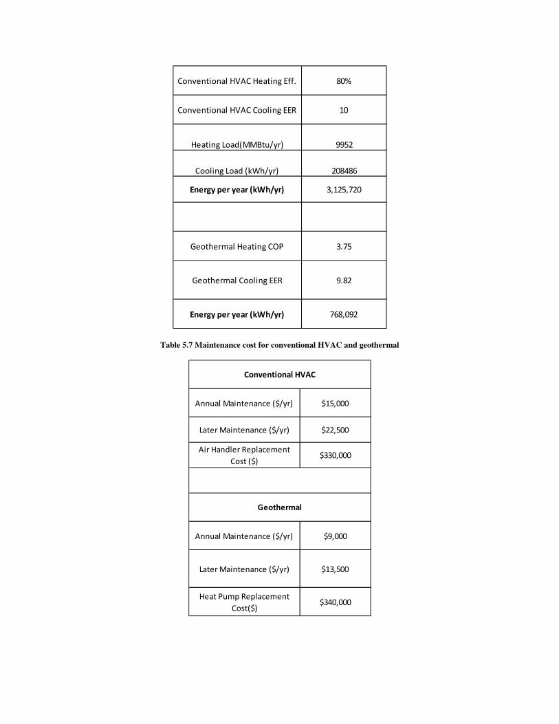
Table 5.6 Energy load and efficiencies for conventional HVAC and geothermal
Economy Inflation (%) Interest (%)
Strong 2.5 4
Nominal 4 6
Poor 7 10
Installation Cost $25,000
Air Handler Cost $330,000
Total Cost $355,000
Bore Field Cost(
including Piping)$3,748,000
Heat Pump Cost $340,000
Total Cost $4,088,000
Geothermal System
Initial Costs
Conventional HVAC System
Initial Costs
Table 5.7 Maintenance cost for conventional HVAC and geothermal
Conventional HVAC Heating Eff. 80%
Conventional HVAC Cooling EER 10
Heating Load(MMBtu/yr) 9952
Cooling Load (kWh/yr) 208486
Energy per year (kWh/yr) 3,125,720
Geothermal Heating COP 3.75
Geothermal Cooling EER 9.82
Energy per year (kWh/yr) 768,092
Annual Maintenance ($/yr) $15,000
Later Maintenance ($/yr) $22,500
Air Handler Replacement
Cost ($)$330,000
Annual Maintenance ($/yr) $9,000
Later Maintenance ($/yr) $13,500
Heat Pump Replacement
Cost($)$340,000
Conventional HVAC
Geothermal
Figure 5.1 Cumulative costs for both the conventional HVAC
Figure 5.2
Figure 5.1 Cumulative costs for both the conventional HVAC and geothermal systems
Figure 5.2 Cumulative costs with high natural gas prices
and geothermal systems
Figure 5.3 Payback Period
6.0 Discussion of Results and Economic Analysis
Due to the size restrictions of the available land, the overall cooling load that is attainable is 600
tons. This value is significantly less than that which is being utilized for the current cooling loads on the
Agricultural Campus. A major benefit of this system is that it will not only be able to provide cooling
energy in the warmer months, but it will also be able to generate approximately 780,000kwh/yr of energy
for heating purposes. The combined ability to heat and cool, operate at a high efficiency, and produce
clean sustainable energy are all very important benefits that would be attained by the installation of this
system.
All the calculated parameters of the borefield are consistent with typical vertical closed loop
geothermal systems. A brief design summary of the system can be seen in Table 7.1. The overall costs
associated with the designed system are comparable to systems of similar size that are currently
operating7. This means that the cost calculations were accurate and provide a good basis for long term
analysis. The operating costs were estimated using several case studies of similar geothermal systems7.
Vertical geothermal HVAC systems have very low operating and maintenance costs due to their simple
design and few moving parts. The only significant operating costs occur from the electricity required to
pump the circulating fluid and the labor to occasionally monitor the system and make sure everything is
working properly. The main maintenance cost stems from leaks in the HDPE pipe resulting from age and
normal wear. These leaks can be somewhat expensive to repair because of the labor involved in removing
the pipe from the bore, repairing the leak, and freshly backfilling the bore.
For economic analysis and to give a comparison between the cumulative costs of a conventional
HVAC system versus the geothermal system, three different cases were presented. These cases compared
the two systems under strong, nominal, and poor economic conditions. The interest and inflation rates for
each economic condition can be seen in Table 5.4. When making this comparison the main components of
each system were given a 20 year lifetime. Regardless of the economic conditions, the geothermal system
had a much higher cumulative cost compared the conventional HVAC system. We also made one more
comparison of the two systems under the assumption of high natural gas prices. Natural gas is currently
used as the main source of heating buildings so if the price of natural gas were to dramatically increase
this would have a significant impact on the feasibility of a geothermal installation. After about 25 years
under a high natural gas price scenario, the geothermal system becomes less expensive than the
conventional system. The results of the comparison can be seen in Figure 5.2. More in depth tables with
all of the values for the comparisons can be seen in the Appendices in tables 11.1 through 11.9. After
determining a total capital cost of about 4 million dollars, the payback period was computed. This system
gives a return of investment by reducing heating and cooling costs in the range of 40 to 60 percent. With
approximate savings at 50% the payback period under a strong economy would come after about twenty
five years and could be as long as thirty years in a poor economy. The results of the payback period
calculation can be seen in figure 5.3 and the yearly data can be seen in Appendices tables 11.10 through
11.12.
Table 6.1 Design Summary Table
Total Length of Borefield 787 feet
Total Width of Borefield 213 feet
Total Number of Boreholes 351
Borehole to Borehole Distance 20.01 feet
Borehole Radius 0.197 feet
Borehole Depth 460.63 feet
Total Borefield Capacity 600 tons
Capital Cost 4.1 million
7.0 Conclusions
Currently, it is not economically feasible to install the designed geothermal system. The
payback period of a feasible capital cost project of this magnitude is between ten to twenty years. The
system that was designed has a payback period of between twenty-five to thirty years. Due to limited
space, the already existing conventional HVAC infrastructure, and the high capital cost associated with
the geothermal system it is a better economic decision to stick with conventional heating and cooling
methods. It would be much more feasible to install a geothermal system if it was under new construction.
If natural gas and electricity prices were to significantly increase, then it would justify retrofitting the
existing heating and cooling system to include a geothermal system. With natural gas prices currently low
the trend only slightly increasing in the future, natural gas appears to be the most economical source of
energy for the foreseeable future. The projections for the price of natural gas can be seen in Figure 8.1.
Although natural gas may be the best source of energy under current conditions, the fact still remains that
natural gas is a non-renewable resource and is not sustainable. With the idea of climate change occurring
due to our strong reliance on fossil fuels there may become many new incentives for sustainable energy
production in the near future. With new incentives to reduce our carbon footprint and invest in sustainable
technology the installation of this geothermal application may become much more feasible in the very
near future.
Figure 7.1 Natural Gas Projected Cost16
8.0 Recommendations
It is our recommendation based on the calculated capital costs and payback period that the system not be installed. If sustainability and public perception of sustainability of the University is of great importance, it would be our recommendation to install one of the three loops. Not only would this allow us to give the geothermal application a good “test,” but it would also decrease the overall capital cost of the project while giving notoriety to the University for increasing the presence of sustainable energy on campus. Due to the major scale of construction and limited parking on the Agricultural Campus, it would be our recommendation that only one loop at a time be installed. This would allow two-thirds of the parking lot to remain in use while construction of the boreholes and piping is being installed. This also allows for future loops to be completed with limited parking interference if gas and electricity prices rise and the University decided to increase its sustainable energy.
9.0 References
1Engineering Services Group design of a ground source heat pump system for the UT sorority village
2Kavanaugh, Stephen P., and Kevin D. Rafferty.Ground-source Heat Pumps: Design of Geothermal
Systems for Commercial and Institutional Buildings. Atlanta: American Society of Heating, Refrigerating
and Air-Conditioning Engineers, 1997. Print. (Design Information)