Design and evaluation of self-optimisation algorithms for ... · PDF fileDesign and evaluation...

Design and evaluation of self-optimisation

algorithms for radio access networks

Orange Labs

Zwi Altman, June 9th 2009, Santander Spain

Orange Labs - Recherche & Développement – Design of SON algorithms – June 09, 20092

Outline

� Introduction:

Control and optimization

� Reinforcement Learning framework

� Case study – LTE ICIC

� Conclusions

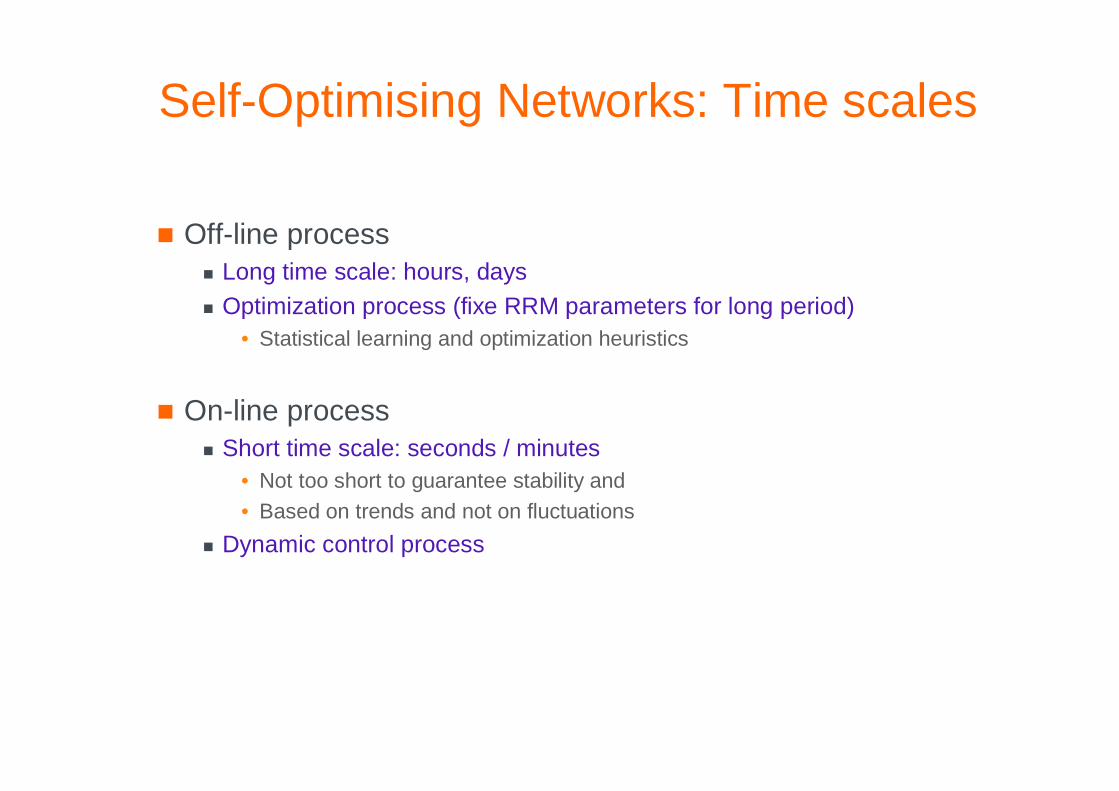
Self-Optimising Networks: Time scales

� Off-line process� Long time scale: hours, days� Optimization process (fixe RRM parameters for long period)

• Statistical learning and optimization heuristics

� On-line process� Short time scale: seconds / minutes

• Not too short to guarantee stability and • Based on trends and not on fluctuations

� Dynamic control process

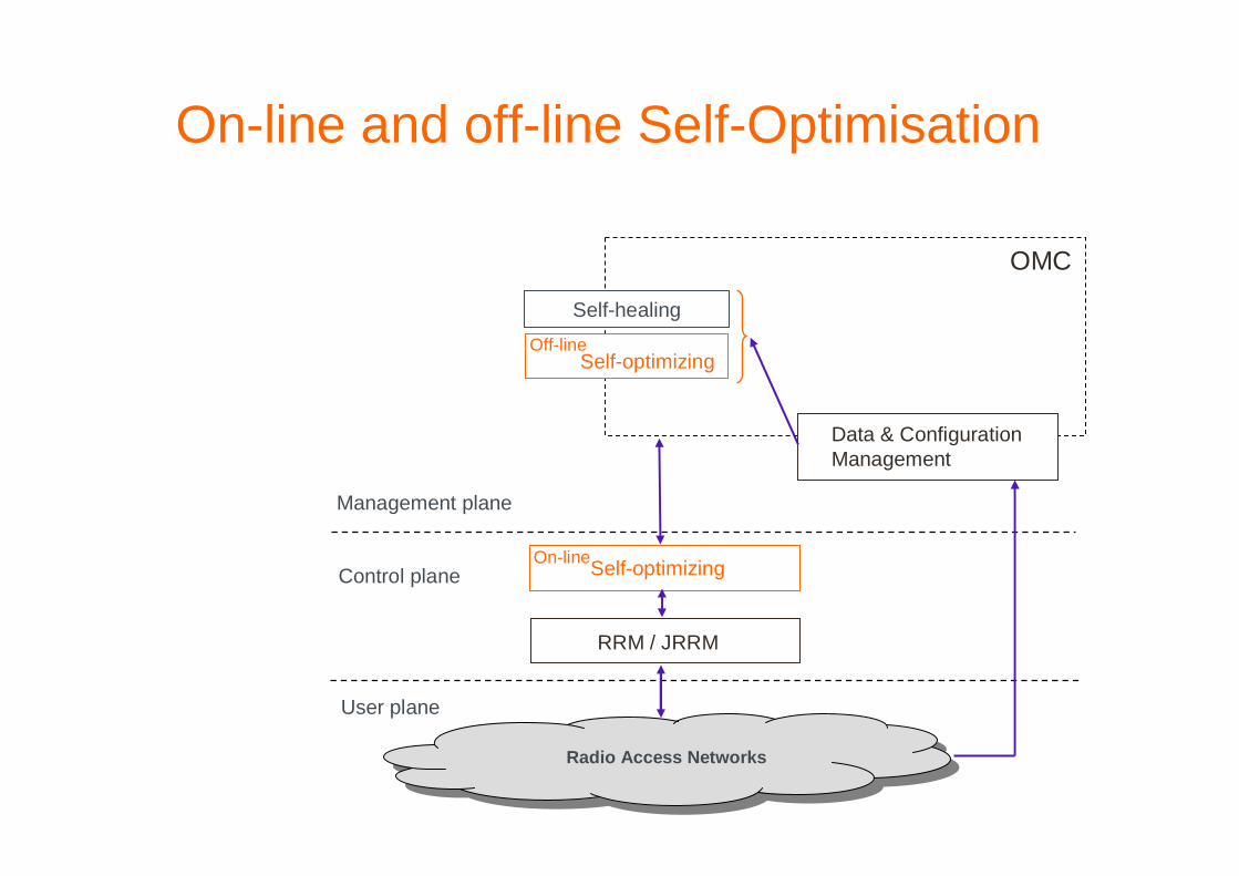
On-line and off-line Self-Optimisation

RRM / JRRM

Radio Access Networks

OMC

User plane

Control plane

Management plane

Self-optimizingOn-line

Self-healing

Self-optimizingOff-line

Data & Configuration Management

Orange Labs - Research & Development – Design of SON Algorithms – Santander, June 9 20095

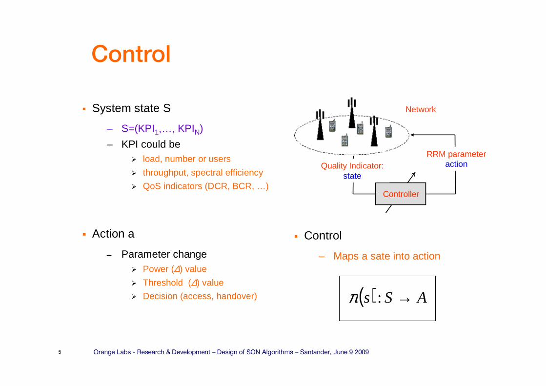
Control

� System state S

– S=(KPI1,…, KPIN)

– KPI could be� load, number or users

� throughput, spectral efficiency

� QoS indicators (DCR, BCR, …)

� Action a

– Parameter change� Power (∆) value

� Threshold (∆) value

� Decision (access, handover)

Controller

Network

RRM parameteractionQuality Indicator:

state

( ) ASs →:π

� Control

– Maps a sate into action


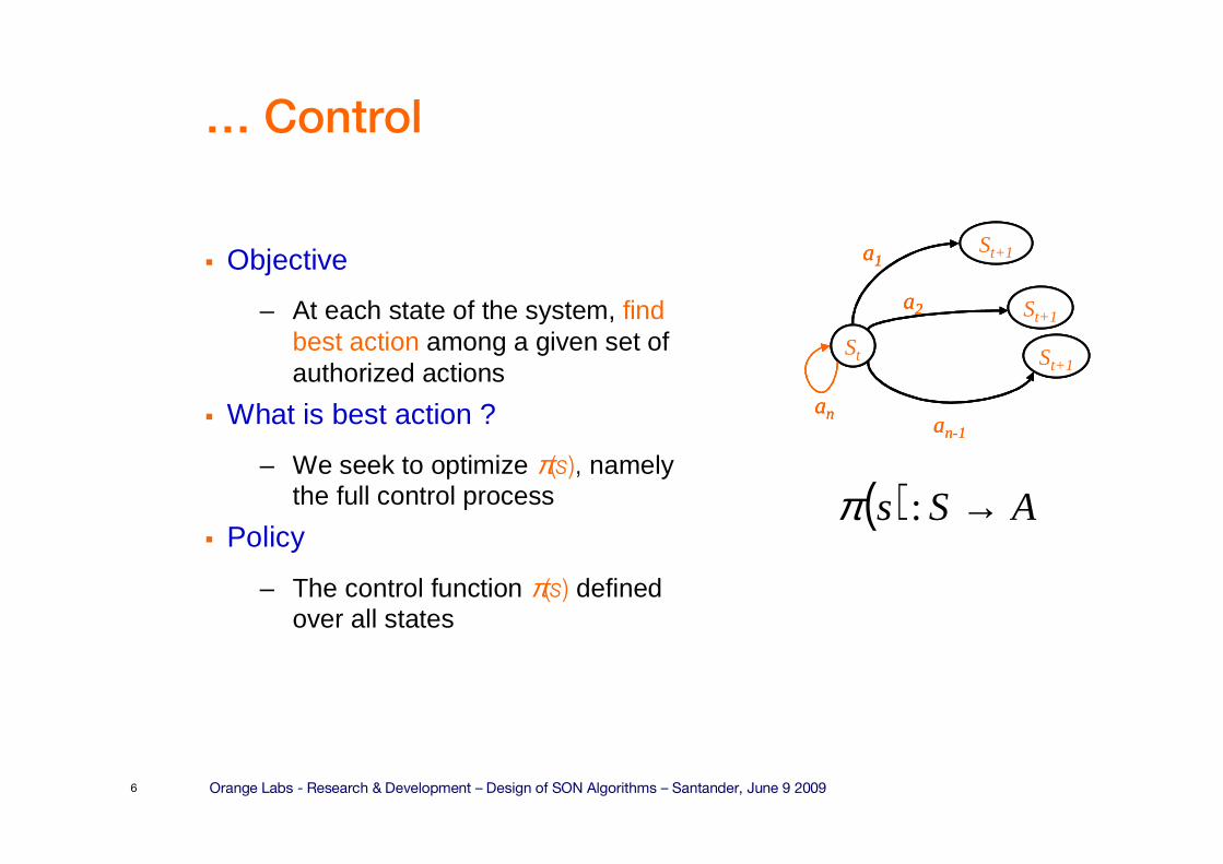
… Control

� Objective

– At each state of the system, find best action among a given set of authorized actions

� What is best action ?

– We seek to optimize π(s), namely the full control process

� Policy

– The control function π(s) defined over all states

St+1

St+1St

an

St+1

a1

a2

an-1

St+1

St+1St

an

St+1

a1

a2

St+1

St+1St

an

St+1

a1

a2

an-1

( ) ASs →:π


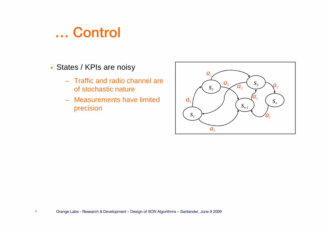
… Control

� States / KPIs are noisy

– Traffic and radio channel are of stochastic nature

– Measurements have limited precision

s2

sn-1

s1

s3

sn

a1

a1

a3

a1

a3

a2

a2

a2

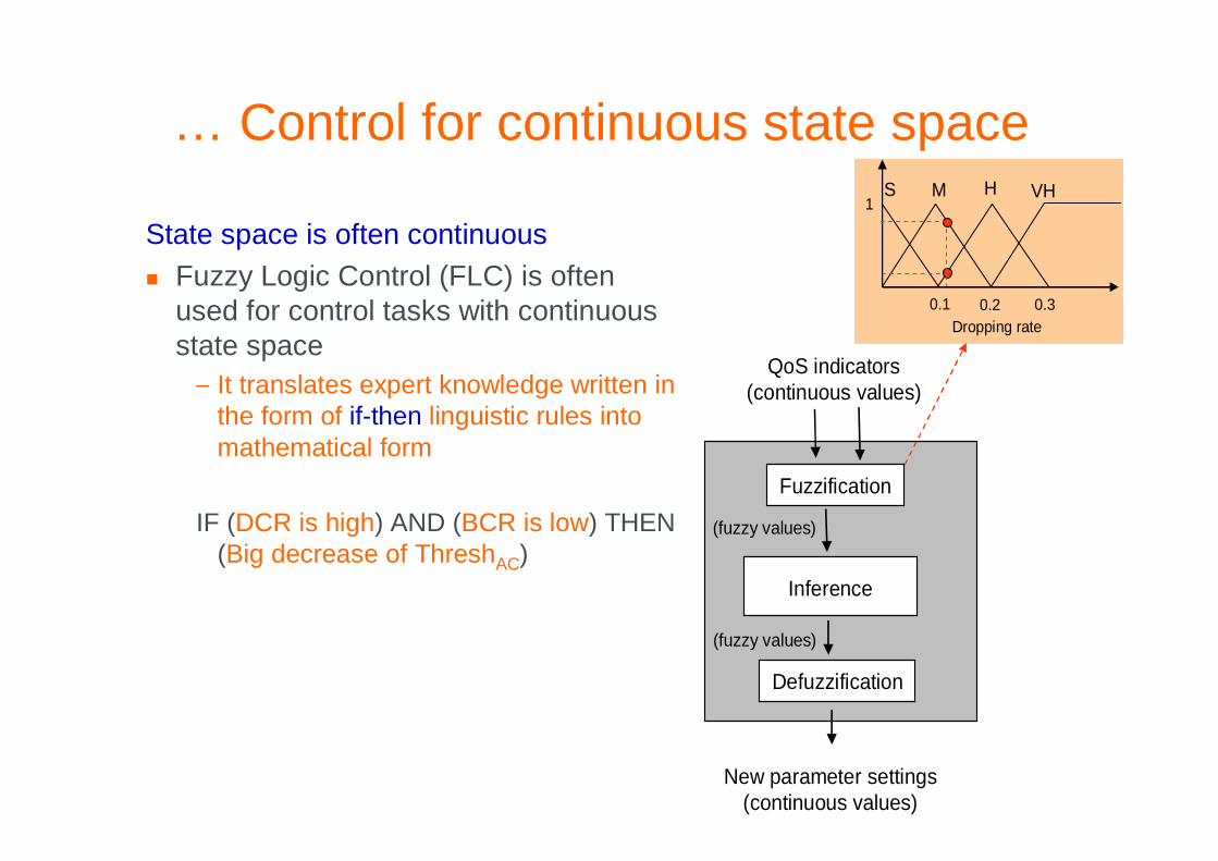
… Control for continuous state space

Fuzzification

Inference

Defuzzification

New parameter settings(continuous values)

QoS indicators(continuous values)

(fuzzy values)

(fuzzy values)

S M H VH1

0.1 0.2 0.3Dropping rate

State space is often continuous

� Fuzzy Logic Control (FLC) is often used for control tasks with continuous state space– It translates expert knowledge written in

the form of if-then linguistic rules into mathematical form

IF (DCR is high) AND (BCR is low) THEN (Big decrease of ThreshAC)

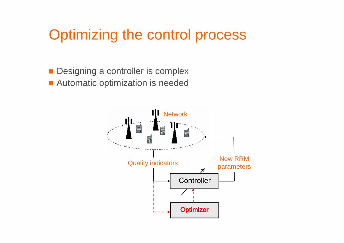
Optimizing the control process

� Designing a controller is complex� Automatic optimization is needed

Network

New RRM parameters

Controller

Quality indicators

OptimizerOptimizerOptimizerOptimizer


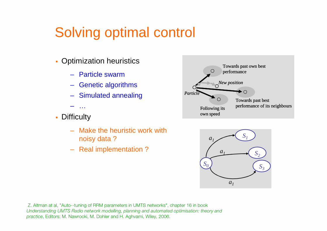
Solving optimal control

� Optimization heuristics

– Particle swarm

– Genetic algorithms

– Simulated annealing

– …

� Difficulty

– Make the heuristic work with noisy data ?

– Real implementation ?

Particle

Following its own speed

Towards past own bestperformance

Towards past bestperformance of its neighbours

New position

Particle

Following its own speed

Towards past own bestperformance

Towards past bestperformance of its neighbours

New position

S1

S3S0

S2

a1

a1

a1

Z. Altman at al, "Auto--tuning of RRM parameters in UMTS networks", chapter 16 in book

Understanding UMTS Radio network modelling, planning and automated optimisation: theory and

practice, Editors: M. Nawrocki, M. Dohler and H. Aghvami, Wiley, 2006.


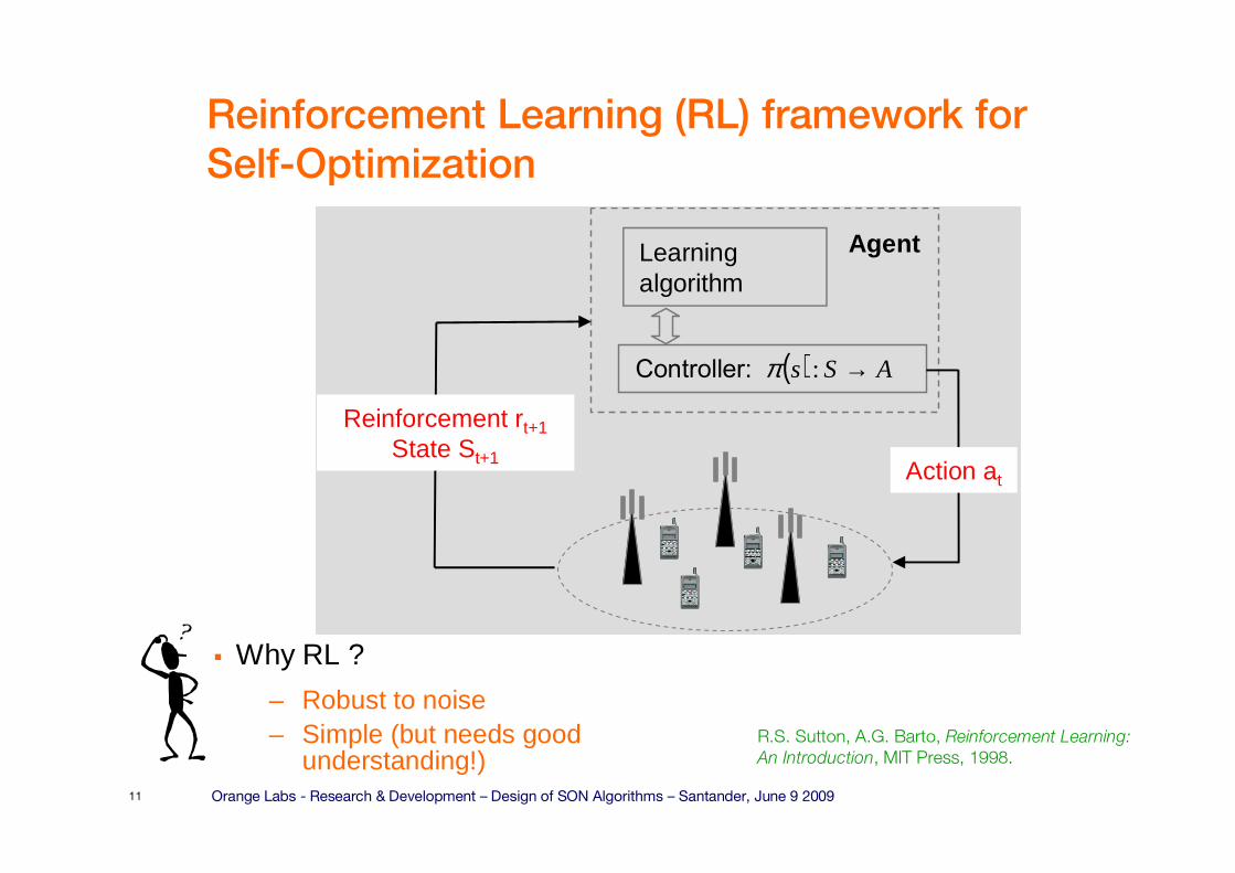
Reinforcement Learning (RL) framework for

Self-Optimization

� Why RL ?

– Robust to noise– Simple (but needs good

understanding!)

Controller:

Learning algorithm

Agent

Action at

Reinforcement rt+1State St+1

( ) ASs →:π

R.S. Sutton, A.G. Barto, Reinforcement Learning:

An Introduction, MIT Press, 1998.


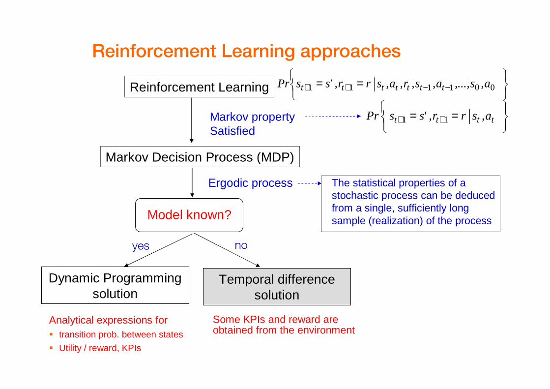
Reinforcement Learning approaches

The statistical properties of a stochastic process can be deduced from a single, sufficiently long sample (realization) of the process

== −−++ 001111 a,s,...,a,s,r,a,srr,'ssPr tttttttReinforcement Learning

Markov Decision Process (MDP)

== ++ tttt a,srr,'ssPr 11Markov propertySatisfied

yes

Ergodic process

Model known?

Dynamic Programmingsolution

Temporal differencesolution

Analytical expressions for� transition prob. between states

� Utility / reward, KPIs

no

Some KPIs and reward are obtained from the environment


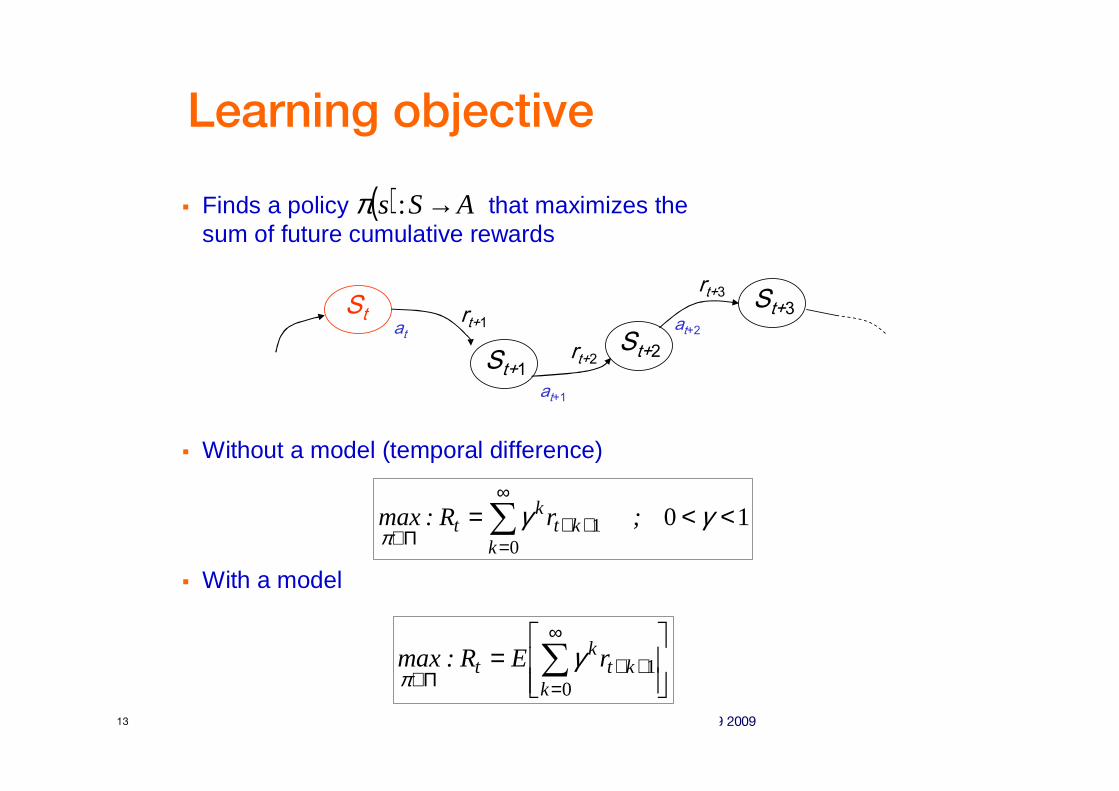
Learning objective

� Finds a policy that maximizes the sum of future cumulative rewards

� Without a model (temporal difference)

� With a model

∑∞

=++

Π∈<<=

01 10

kkt

kt ;rR:max γγ

π

St

St+1

rt+1St+2

St+3

rt+2

rt+3

at

at+1

at+2

= ∑

∞

=++

Π∈ 01

kkt

kt rER:max γ

π

( ) ASs →:π


Q-algorithm

( ) ( )a,sQmaxra,sQ tta

tttt ′+= +′++ 111 γ

� We choose an action at, and continue with the (up to now) best policy

� Q-function

� To guarantee convergence: add a learning rate coefficient η

( ) ( ) ( ) ( )

( ) ( ) ( )( ) 1

11

111 1

+

+′+

+′++

∆+=

−′++=

′++−=

tttt

ttttta

tttt

tta

ttttttt

Qa,sQ

a,sQa,sQmaxra,sQ

a,sQmaxra,sQa,sQ

γη

γηη

starting from (st,at)( ) ( ) ∑∞

=++==

01

kkt

ktttttt ra,sRa,sQ γ


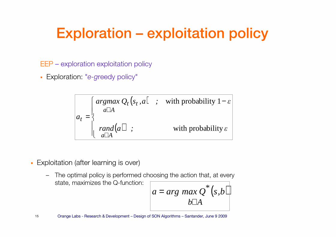
Exploration – exploitation policy

� Exploitation (after learning is over)

– The optimal policy is performed choosing the action that, at every

state, maximizes the Q-function:

( )Ab

* b,sQmaxarga∈

=

EEP – exploration exploitation policy

� Exploration: "e-greedy policy"

( )

( )

−

=

∈

∈

ε ;arand

ε;a,sQargmax

a

Aa

ttAa

t

bilitywith proba

bility 1with proba


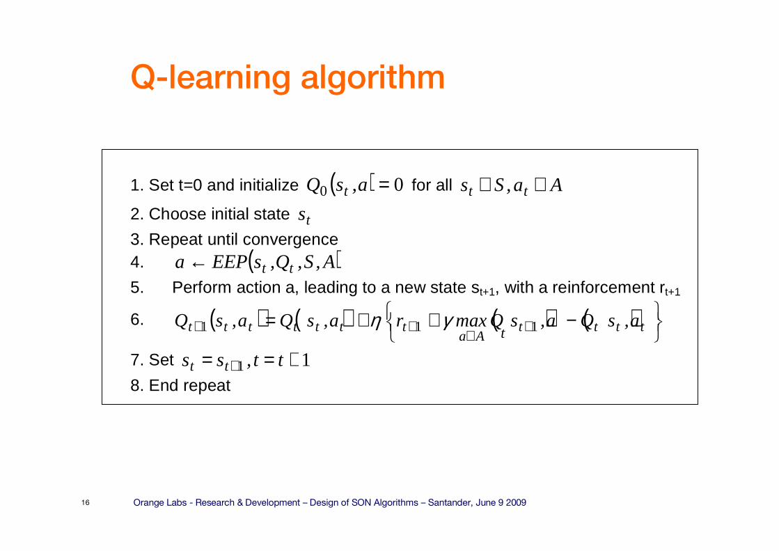
Q-learning algorithm

1. Set t=0 and initialize ( ) 00 =a,sQ t for all Aa,Ss tt ∈∈

2. Choose initial state ts

3. Repeat until convergence 4. ( )A,S,Q,sEEPa tt←

5. Perform action a, leading to a new state st+1, with a reinforcement rt+1

6. ( ) ( ) ( ) ( )

−++= +

∈++ tttt

Aattttttt a,sQa,sQmaxra,sQa,sQ 111 γη

7. Set 11 +== + tt,ss tt

8. End repeat

t


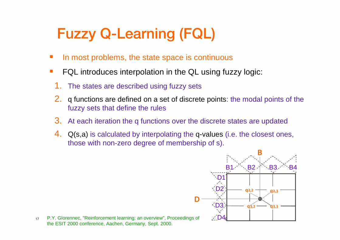
Fuzzy Q-Learning (FQL)

� In most problems, the state space is continuous

� FQL introduces interpolation in the QL using fuzzy logic:

1. The states are described using fuzzy sets

2. q functions are defined on a set of discrete points: the modal points of the fuzzy sets that define the rules

3. At each iteration the q functions over the discrete states are updated

4. Q(s,a) is calculated by interpolating the q-values (i.e. the closest ones, those with non-zero degree of membership of s).

B1 B2 B3 B4

D1

D2

D3

D4

q2,2

q3,3

q2,3

q3,2

B

P.Y. Glorennec, "Reinforcement learning: an overview", Proceedings of the ESIT 2000 conference, Aachen, Germany, Sept. 2000.

D

… Fuzzy Q-learning

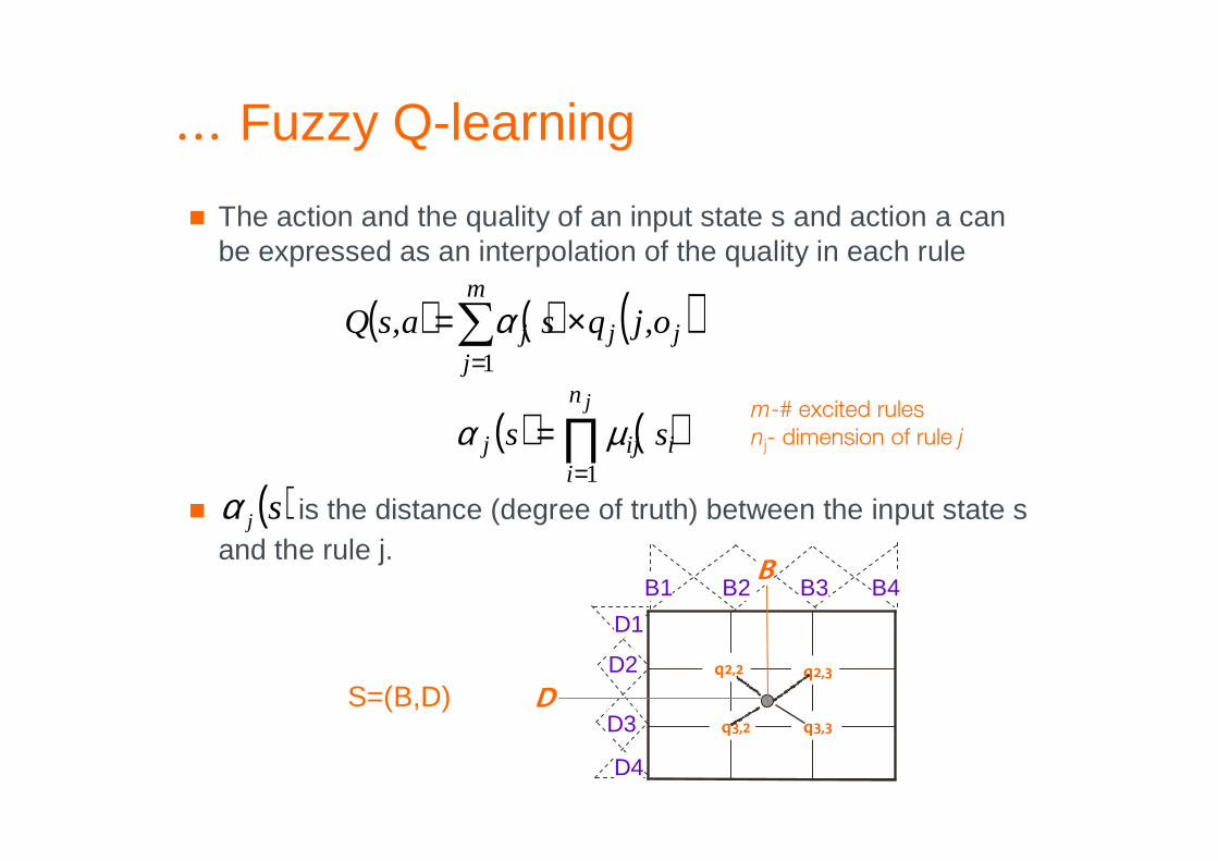
� The action and the quality of an input state s and action a can be expressed as an interpolation of the quality in each rule

� is the distance (degree of truth) between the input state s and the rule j.

S=(B,D)

B1 B2 B3 B4

D1

D2

D3

D4

q2,2

q3,3

q2,3

q3,2

B

D

m-# excited rules

nj- dimension of rule j

( )sjα

( ) ( ) ( )∑=

×=m

jjjj o,jqsa,sQ

1

α

( ) ( )∏=

=jn

iiijj ss

1

µα

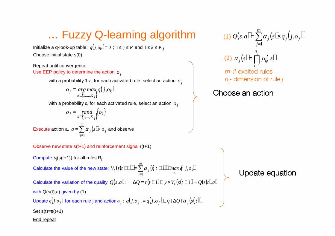
Initialize a q-look-up table: ( ) 0=ko,jq ; Rj ≤≤1 and jKk ≤≤1

Choose initial state s(0) Repeat until convergence Use EEP policy to determine the action jo

with a probability 1-ε, for each activated rule, select an action jo

{ }

( )kK,...,k

j o,jqmaxargoj1∈

=

with a probability ε, for each activated rule, select an action jo

{ }{ }kK,...,k

j orandoj1∈

=

Execute action a, ( )∑=

×=m

jjj osa

1

α and observe

Observe new state s(t+1) and reinforcement signal r(t+1)

Compute αj(s(t+1)) for all rules Rj

Calculate the value of the new state: ( )( ) ( )( ) ( )∑=

⋅+=+m

jkjt o,jqmaxtstsV

1 k

11 α

Calculate the variation of the quality ( )a,sQ : ( ) ( )( ) ( )( )a,tsQtsVtrQ t −+×++=∆ 11 γ

with Q(s(t),a) given by (1)

Update ( )jo,jq for each rule j and action jo : ( ) ( ) ( )( )tsQo,jqo,jq jjj αη ⋅∆⋅+= .

Set s(t)=s(t+1)

End repeat

… Fuzzy Q-learning algorithm

ChooseChooseChooseChoose an actionan actionan actionan action

Update equationUpdate equationUpdate equationUpdate equation

( ) ( ) ( )∑=

×=m

jjjj o,jqsa,sQ

1

α(1)

( ) ( )∏=

=jn

iiijj ss

1

µα(2)

m-# excited rules

nj- dimension of rule j

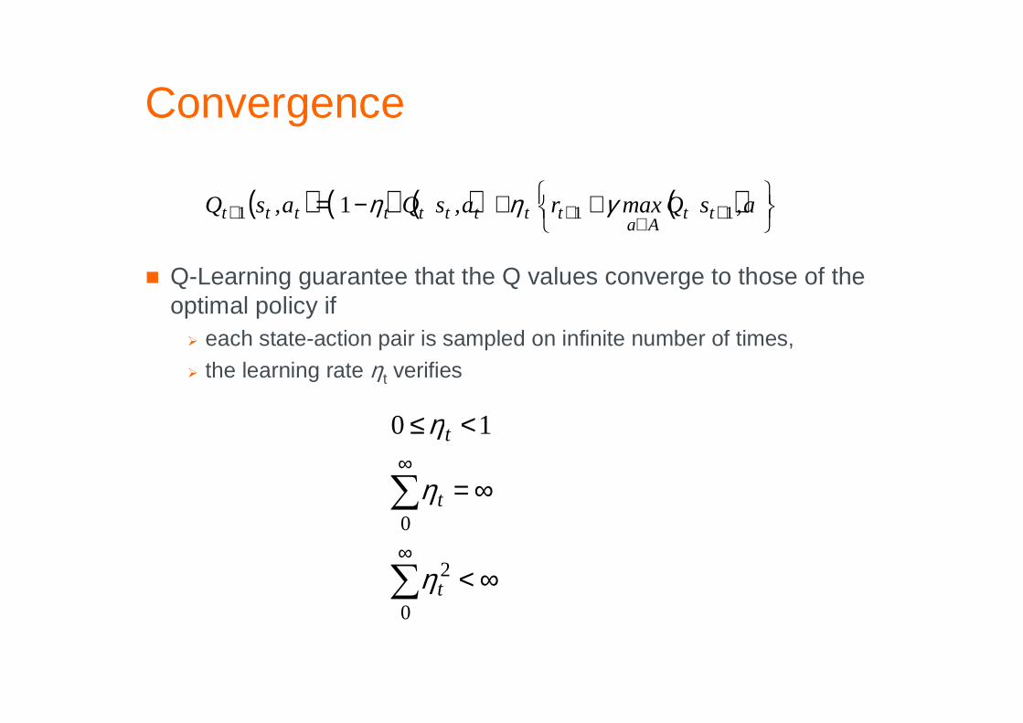
Convergence

� Q-Learning guarantee that the Q values converge to those of the optimal policy if

� each state-action pair is sampled on infinite number of times,

� the learning rate ηt verifies

( ) ( ) ( ) ( )

++−= +

∈++ a,sQmaxra,sQa,sQ tt

Aattttttttt 111 1 γηη

∑

∑

∞

∞

∞<

∞=

<≤

0

2

0

10

t

t

t

η

η

η

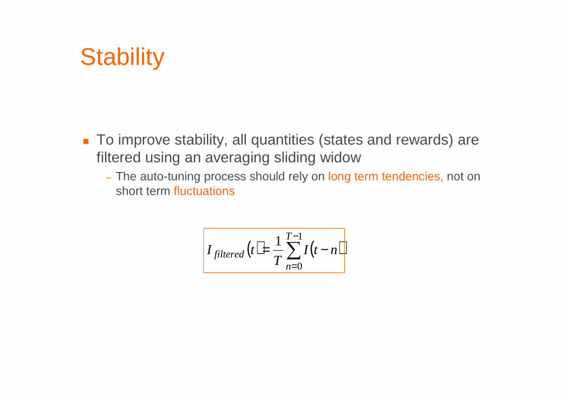
Stability

( ) ( )∑−

=−=

1

0

1 T

nfiltered ntI

TtI

� To improve stability, all quantities (states and rewards) are filtered using an averaging sliding widow

– The auto-tuning process should rely on long term tendencies, not on short term fluctuations


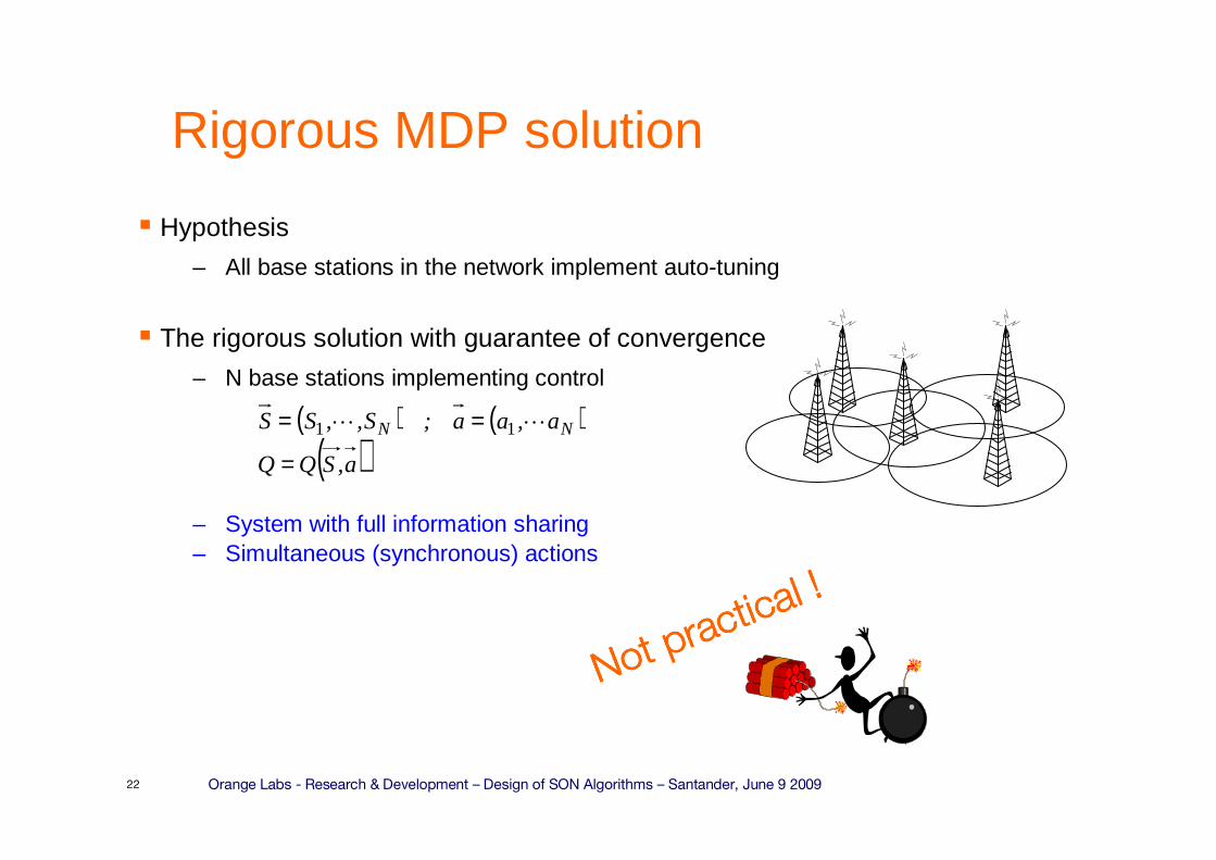
Rigorous MDP solution

� Hypothesis

– All base stations in the network implement auto-tuning

� The rigorous solution with guarantee of convergence

– N base stations implementing control

– System with full information sharing– Simultaneous (synchronous) actions

( ) ( )( )a,SQQ

a,aa;S,,SS NN

=

== LL 11

Not pr

actical

!

Not pr

actical

!

Not pr

actical

!

Not pr

actical

!


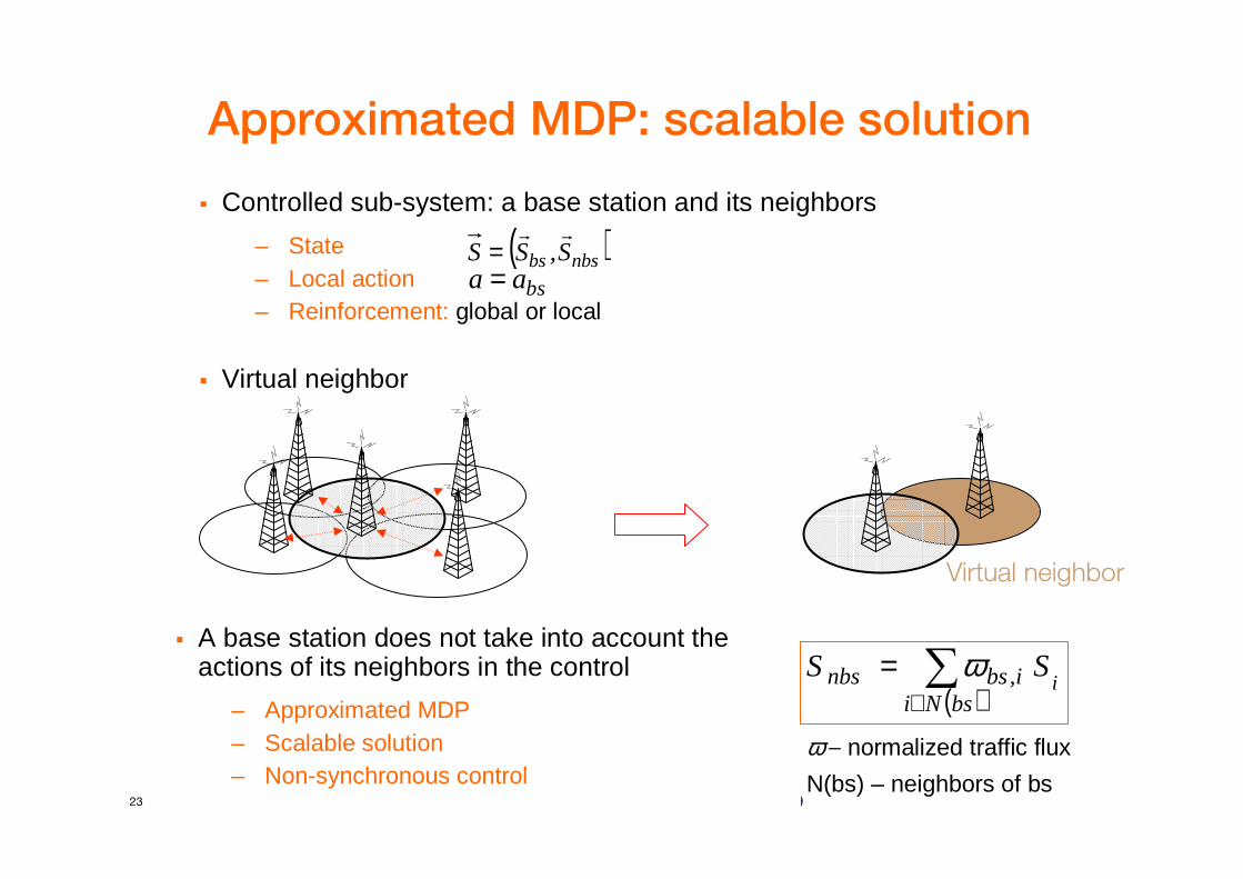
Approximated MDP: scalable solution

� Controlled sub-system: a base station and its neighbors

– State– Local action– Reinforcement: global or local

� Virtual neighbor

( )nbsbs S,SSrr

=bsaa =

Virtual neighbor

( )∑

∈=

bsNii,bsnbs i

SS ω� A base station does not take into account the

actions of its neighbors in the control

– Approximated MDP– Scalable solution– Non-synchronous control

ω – normalized traffic flux

N(bs) – neighbors of bs


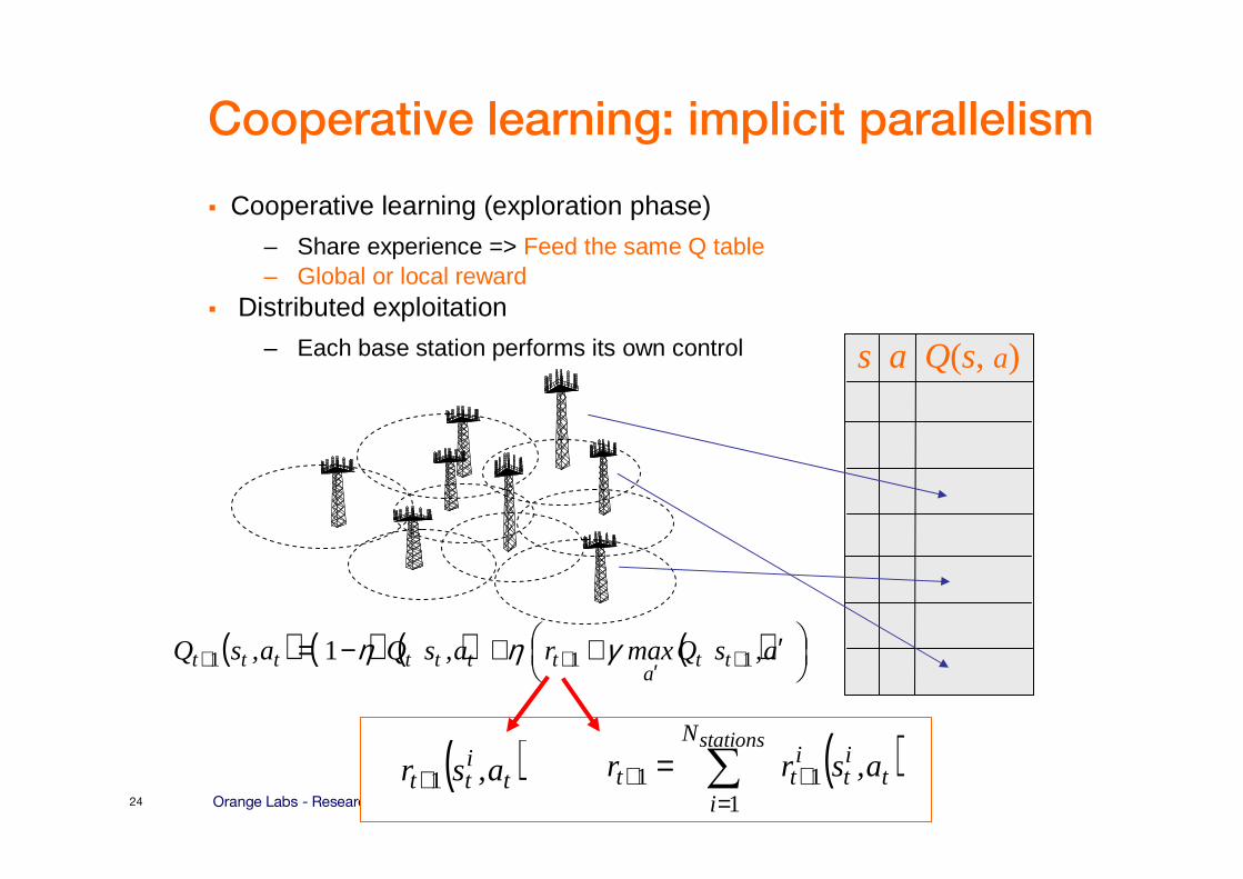
Cooperative learning: implicit parallelism

� Cooperative learning (exploration phase)

– Share experience => Feed the same Q table– Global or local reward

� Distributed exploitation

– Each base station performs its own control

( )∑=

++ =stationsN

it

it

itt a,srr

111

s a Q(s, a)

( ) ( ) ( ) ( )

′++−= +′++ a,sQmaxra,sQa,sQ tt

attttttt 111 1 γηη

( )titt a,sr 1+


Use case

� SON use cases studied

– Admission control (UMTS)

– Mobility (UMTS)

– RT and NRT resource allocation (UMTS)

– Mobility in heterogeneous network (UMTS-WLAN)

– Mobility (LTE)

– DL ICIC (LTE)

– UL Power control / ICIC (LTE)

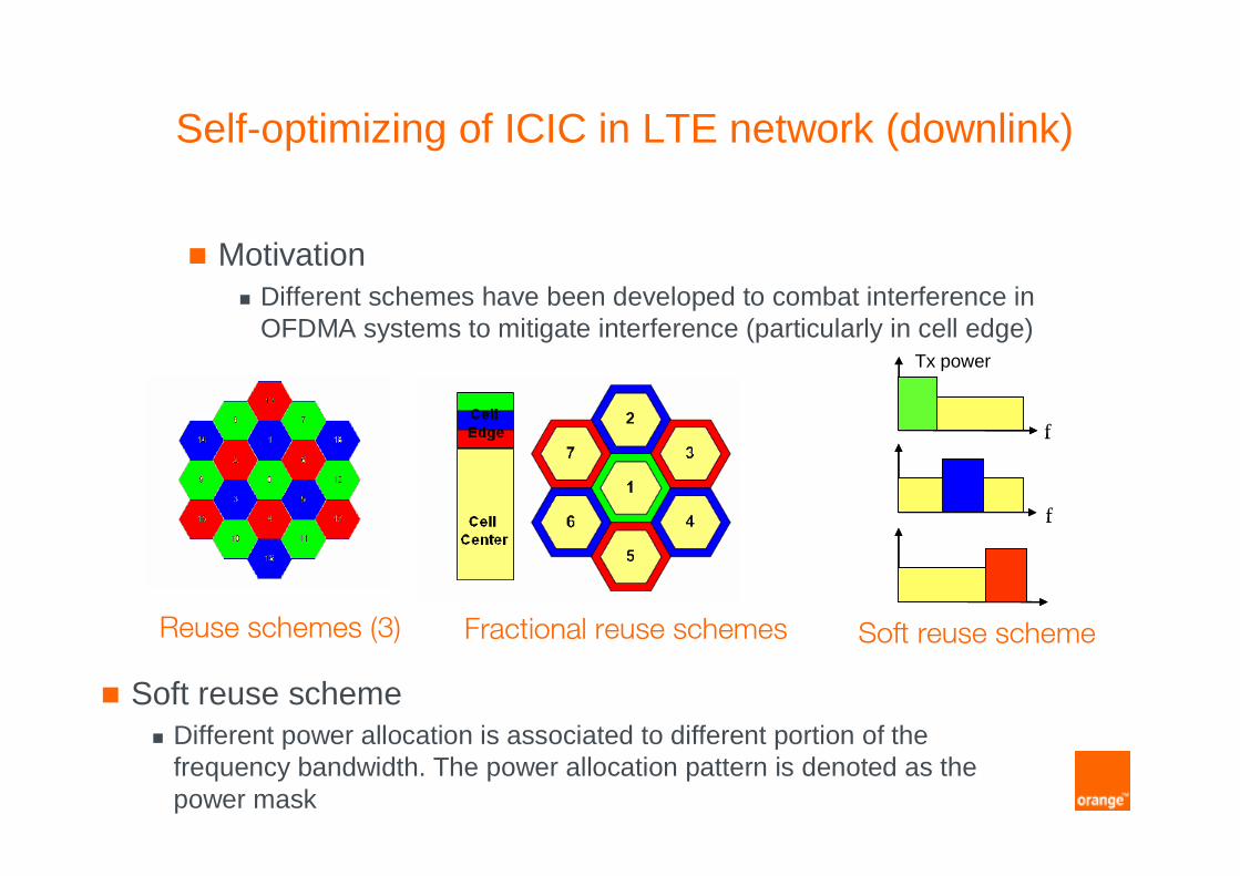
Self-optimizing of ICIC in LTE network (downlink)

� Motivation� Different schemes have been developed to combat interference in

OFDMA systems to mitigate interference (particularly in cell edge)

Reuse schemes (3) Fractional reuse schemes

f

f

Tx power

f

f

Tx power

Soft reuse scheme

� Soft reuse scheme� Different power allocation is associated to different portion of the

frequency bandwidth. The power allocation pattern is denoted as the power mask

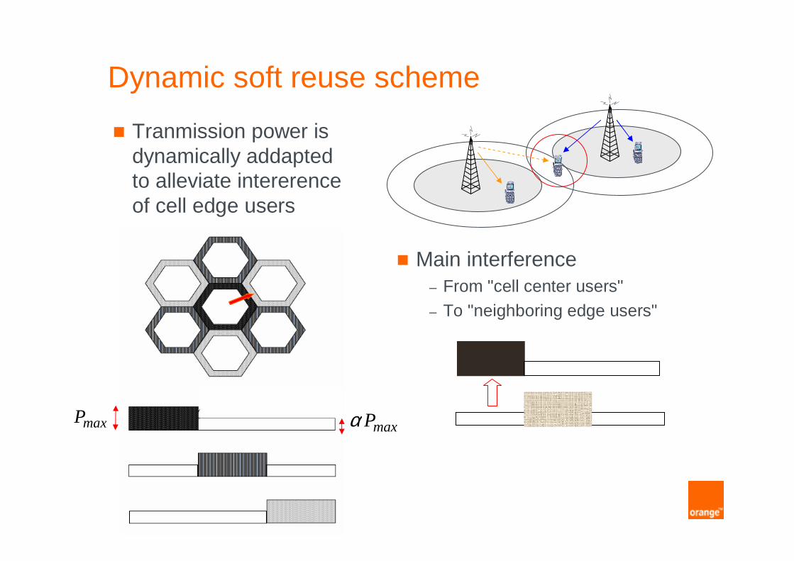
Dynamic soft reuse scheme

maxP

� Tranmission power is dynamically addaptedto alleviate intererenceof cell edge users

� Main interference– From "cell center users"– To "neighboring edge users"

maxPα

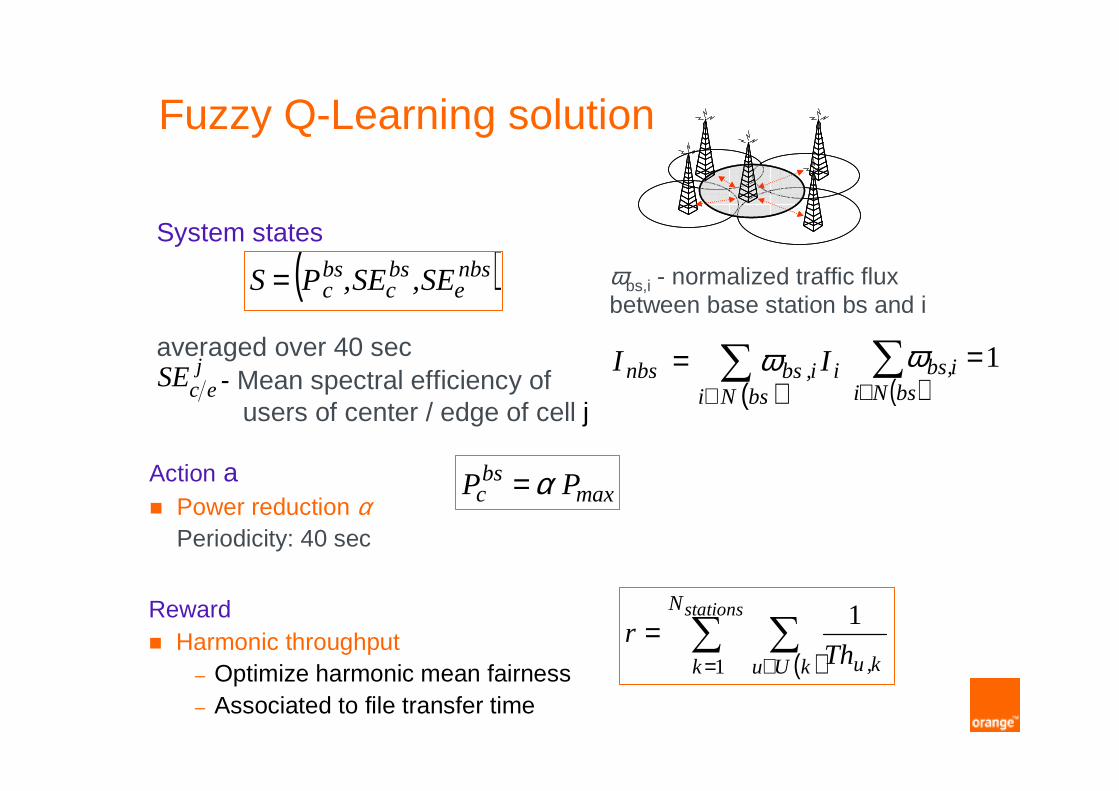
Fuzzy Q-Learning solution

System states

averaged over 40 sec- Mean spectral efficiency of

users of center / edge of cell j

( )nbse

bsc

bsc SE,SE,PS= ωbs,i - normalized traffic flux

between base station bs and i

Action a� Power reduction α

Periodicity: 40 sec

Reward� Harmonic throughput

– Optimize harmonic mean fairness– Associated to file transfer time

( )∑

∈=

bsNiii,bsnbs II ω

( )∑

∈=

bsNii,bs 1ω

( )∑ ∑

= ∈=

stationsN

k kUu k,uThr

1

1

maxbsc PP α=

jecSE

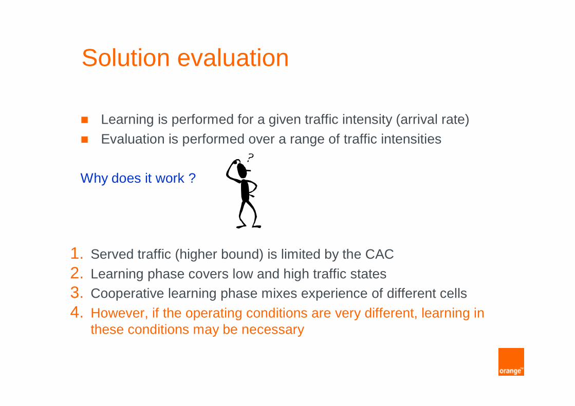
Solution evaluation

� Learning is performed for a given traffic intensity (arrival rate)

� Evaluation is performed over a range of traffic intensities

Why does it work ?

1. Served traffic (higher bound) is limited by the CAC

2. Learning phase covers low and high traffic states3. Cooperative learning phase mixes experience of different cells

4. However, if the operating conditions are very different, learning in these conditions may be necessary

Results Reuse-3

M. Dirani, Z. Altman, "A cooperative Reinforcement Learning approach for inter-cell interference

coordination in OFDMA cellular networks", submitted

Results

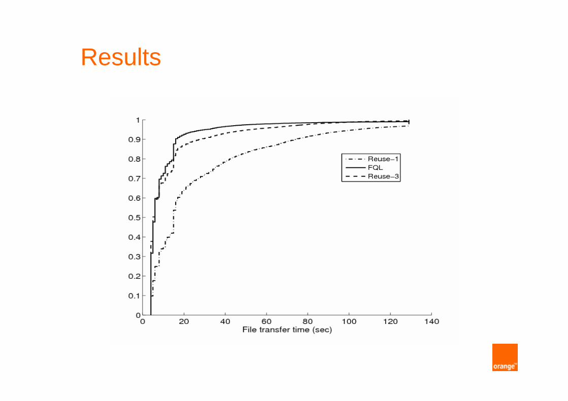
Results


Conclusions

� Reinforcement Learning provides a robust and simple framework for designing self-optimizing functions

– Simple to implement

– Robust with respect to noise introduced by traffic and propagation fluctuations

� Future directions / challenges

� Simplified learning algorithms to implement in real networks

� Further distribution of the control to allow coordinated operation of SON entities

– Game/team theory approaches

Date post:	31-Jan-2018
Category:	Documents
Upload:	vankiet
View:	221 times
Download:	0 times

Design and evaluation of self-optimisation algorithms for ... · PDF fileDesign and evaluation...

Documents