Page 1
DESIGN AND FABRICATION OF AN ELBOW MOTION SIMULATOR
by
Joshua P. Magnusen
B. S. in Mechanical Engineering, Pennsylvania State University, 2002
Submitted to the Graduate Faculty of
The School of Engineering in partial fulfillment
of the requirements for the degree of
Master of Science in Mechanical Engineering
University of Pittsburgh
2004
Page 2
UNIVERSITY OF PITTSBURGH
SCHOOL OF ENGINEERING
This thesis was presented
by
Joshua P. Magnusen
It was defended on
August 3, 2004
and approved by
Jeffrey S. Vipperman, PhD., Assistant Professor, Mechanical Engineering
Mark C. Miller, PhD., Assistant Professor, Mechanical Engineering
Patrick Smolinski, PhD., Associate Professor, Mechanical Engineering
Thesis Advisor: Jeffrey S. Vipperman, Ph. D., Assistant Professor, Mechanical Engineering
ii
Page 3
ABSTRACT
DESIGN AND FABRICATION OF AN ELBOW MOTION SIMULATOR
Joshua P. Magnusen, MS
University of Pittsburgh, 2004
Uncertainty and a lack of knowledge regarding restoration of proper function following an elbow
injury create a need for expanding the understanding of elbow operation. An elbow motion
simulator that is capable of producing motion in a cadaver forearm is designed and developed.
This device will advance the capabilities of similar preceding elbow simulators by physically
simulating the full range of motion and force-loading conditions in the elbow. Electric cylinders
are used to simulate the muscles. The five muscles that are modeled are the biceps, brachialis,
triceps, brachioradialis, and pronator teres. A braided cable attached to the cylinders inserts on
the arm at each muscle’s tendonous insertion. Custom-designed pulley systems are developed
for the muscles to maintain an accurate line of action within the cable by preserving a
physiological moment arm about the joint of rotation. The arm specimen is secured by means
of a humeral clamp that holds the humeral shaft secure during experimentation. The device can
be rotated to test in either a varus or a valgus orientation. Preliminary testing with a wooden arm
model is performed to verify the simulator’s capabilities.
iii
Page 4
TABLE OF CONTENTS 1.0 INTRODUCTION..................................................................................................................1
1.1 MOTIVATION................................................................................................................1
1.2 BRIEF OVERVIEW OF JOINT SIMULATORS ...........................................................5
1.3 CONTRIBUTIONS OF THIS WORK ............................................................................6
2.0 JOINT SIMULATORS .........................................................................................................7
2.1 OVERVIEW ....................................................................................................................7
2.2 UNIVERSITY OF WESTERN ONTARIO ELBOW SIMULATOR.............................8
2.3 SYRACUSE UNIVERSITY WRIST SIMULATOR....................................................10
2.4 PROPOSED SIMULATOR...........................................................................................11
3.0 SURVEY OF PHYSIOLOGIC KINEMATIC DATA......................................................12
3.1 MOMENT ARMS .........................................................................................................12
3.2 RELEVANT ANGLES..................................................................................................15
4.0 SIMULATOR DESIGN.......................................................................................................23
4.1 FRAME DESIGN ..........................................................................................................24
4.2 CABLE SYSTEM DESIGN..........................................................................................28
4.2.1 “Upper-Level” Pulleys.......................................................................................... 28
4.2.2 Triceps Pulleys...................................................................................................... 31
4.2.3 “Lower-Level” Pulleys ......................................................................................... 33
4.2.4 Pulley Selection .................................................................................................... 36
iv
Page 5
4.2.5 Cable Selection ..................................................................................................... 36
4.3 CONTROL SYSTEM....................................................................................................37
4.3.1 Hardware............................................................................................................... 39
4.3.1.1 Compumotor Hardware .................................................................................... 39
4.3.1.2 Secondary Breakout Box .................................................................................. 39
4.3.2 Software ................................................................................................................ 41
5.0 FULFILLING KINEMATIC REQUIREMENTS............................................................43
5.1 SIMULATOR MOMENT ARMS .................................................................................43
5.2 OPERATION VERIFICATION....................................................................................50
6.0 CONCLUSIONS AND FUTURE WORK.........................................................................53
6.1 SUMMARY...................................................................................................................53
6.2 ELBOW FUNCTION ....................................................................................................54
6.3 DYNAMIC STUDIES...................................................................................................54
6.4 NEURAL CONTROL STUDIES..................................................................................55
APPENDIX A: HARDWARE CONNECTION DETAILS .....................................................56
APPENDIX B: DIMENSIONS OF PULLEY POSITIONS ....................................................57
APPENDIX C: FLOWCHART FOR MOMENT ARM CALCULATION ...........................60
APPENDIX D: MATLAB™ CODE FOR ANGULAR DATA................................................61
APPENDIX E: MATLAB™ CODE FOR MOMENT ARM DATA.......................................65
APPENDIX F: SINUSOIDAL MOVEMENTS IN TWO CYLINDERS................................66
BIBLIOGRAPHY........................................................................................................................68
v
Page 6
LIST OF TABLES Table 1: Primary elbow muscles and their roles in motions........................................................... 4
Table 2: Elbow muscle origins and insertions [44] ...................................................................... 17
Table 3: Virtual muscle origins in the elbow simulator................................................................ 44
Table 4: DB37 to Acroloop card connections............................................................................... 56
vi
Page 7
LIST OF FIGURES Figure 1: Forearm flexion-extension [18]....................................................................................... 3
Figure 2: Forearm pronation-supination [18] ................................................................................. 4
Figure 3: Biceps moment arms ..................................................................................................... 13
Figure 4: Brachialis moment arms................................................................................................ 13
Figure 5: Triceps moment arms .................................................................................................... 14
Figure 6: Brachioradialis moment arms........................................................................................ 14
Figure 7: Pronator teres moment arms.......................................................................................... 15
Figure 8: Pulley cable alignment .................................................................................................. 16
Figure 9: Humeral coordinate system [44] ................................................................................... 18
Figure 10: Change in biceps angle through flexion-extension in coronal plane........................... 19
Figure 11: Change in brachialis angle through flexion-extension in coronal plane ..................... 20
Figure 12: Change in triceps angle through flexion-extension in coronal plane .......................... 20
Figure 13: Change in brachioradialis angle through pronation-supination .................................. 21
Figure 14: Change in pronator teres angle through pronation-supination .................................... 22
Figure 15: Completed elbow simulator......................................................................................... 24
Figure 16: Specimen clamping system ......................................................................................... 26
Figure 17: Frame rotation guide ................................................................................................... 27
Figure 18: “Upper-level” secondary pulley (top face removed)................................................... 28
Figure 19: “Center-alignment secondary” pulleys........................................................................ 29
vii
Page 8
Figure 20: “Upper-level” primary pulley...................................................................................... 30
Figure 21: Secondary triceps pulley (front face removed) ........................................................... 32
Figure 22: Primary triceps pulley ................................................................................................. 33
Figure 23: “Lower-level” secondary pulleys (front face removed) .............................................. 34
Figure 24: “Lower-level” primary pulleys.................................................................................... 35
Figure 25: Control system setup ................................................................................................... 38
Figure 26: Axis 1 connections in secondary breakout box ........................................................... 41
Figure 27: Biceps moment arm results ......................................................................................... 44
Figure 28: Brachialis moment arm results .................................................................................... 45
Figure 29: Triceps moment arm results ........................................................................................ 45
Figure 30: Brachioradialis moment arm results............................................................................ 46
Figure 31: Pronator teres moment arm results.............................................................................. 46
Figure 32: Range of biceps’ moment arms ................................................................................... 47
Figure 33: Range of brachialis’ moment arms.............................................................................. 48
Figure 34: Range of pronator teres’ moment arms ....................................................................... 48
Figure 35: Range of brachioradialis’ moment arms ..................................................................... 49
Figure 36: Mock wooden arm for testing ..................................................................................... 51
Figure 37: Frame front view ......................................................................................................... 57
Figure 38: Frame right view ......................................................................................................... 58
Figure 39: Frame top view............................................................................................................ 59
Figure 40: Moment arm calculation flowchart ............................................................................. 60
viii
Page 9
ACKNOWLEDGEMENTS
First of all, I would like to thank my thesis advisor, Dr. Jeffrey Vipperman for his continued
support and motivation when I needed it the most, and for never giving up on me. Secondly, I’d
like to thank my research advisor, Dr. Mark Miller, and Karol Galik, Derek Dazen, and Scott
Kramer from Allegheny General Hospital for their contributions to this work. Thanks to my
committee members Dr. Patrick Smolinski, Dr. Vipperman, and Dr. Miller for their participation
in the defense of this thesis. Special thanks to Pete Bisnette who did a terrific job not only in
constructing the simulator, but for helping with many design issues that were resolved better than
we could have hoped for. I’d like to thank my friends and my family for supporting me,
especially my parents, who have always been an amazing source of inspiration and guidance for
me. Last, but certainly not least, I’d like to thank my better half, Becca, for her patience, love,
and encouragement throughout these past two years. In loving memory of Ianer M. Munck.
ix
Page 10
1.0 INTRODUCTION
1.1 MOTIVATION Injuries of the elbow can be attributed to any number of causes, such as trauma, overuse, and
sports injuries, and can require a person to miss work, often restricting his or her ability to
perform basic functions. Elbow fractures, usually a result of trauma or an athletic injury, will
sometimes merit an elbow replacement. In adults, fractures of the radial head, typically caused
by a fall onto the outstretched hand, represent 5% of all fractures, and approximately 33% of all
elbow fractures [1, 2]. Effective restoration of a fractured radial head has proven quite difficult.
Among the options are internal fixation, excision, or excision and replacement of the radial head.
Which of these methods lends the best results is still very much in question.
When valgus loads are applied to an elbow, the medial collateral ligament (MCL) is the
primary provision of stability in the arm, and the radial head is secondary [3, 4]. Activities such
as pitching in baseball can cause serious injuries to the MCL, at which point the role of the radial
head becomes more essential in elbow stability. Additionally, the radial head aids in both
providing an anterior support for the humerus and in preventing the radius from migrating
proximally with respect to the ulna [5, 6, 7, 8, 9]. Fractures of the radial head may decrease the
stability of the radiocapitellar joint, resulting in radiocapitellar subluxation, which could lead to
painful clicking and secondary osteoarthritis [10].
1
Page 11
The radial head’s biomechanical significance is clear, and it follows thusly that the
importance of an expeditious and effective treatment of its fracture is a major concern. There
has been a great deal of debate over which technique for treating radial head injuries produces
the most optimal results. Typically, displaced radial head fractures are reduced and internally
stabilized, but it has been shown that this method of treatment can result in less than satisfactory
outcomes. Excision of the radial head has been a means of treating a comminuted fracture, but
patients have complained of an unstable elbow and chronic wrist pain [9, 11]. Several radial
head prostheses have been developed in an order to restore active elbow motion to severely
fractured radial heads. Radial head replacement is also called for when there is a comminuted
fracture of the radial head, especially when the elbow has undergone a complex injury [12].
However, the recipients often report complications after they receive the replacement [12].
The forearm is vital to the everyday functionality of humans, from carrying heavy objects
to simply taking a drink of water, and the loss of its use would seriously debilitate an individual.
Past studies have focused on the identifying the geometrical properties of the elbow-forearm
complex, and have laid the groundwork for understanding the basis of forearm movement [7, 13,
14].
Accurate modeling of the muscle forces in the arm is a complex one. The bones of the
forearm, the radius and ulna, are connected to the upper arm, the humerus, by a series of
ligaments and muscles. A simple, but realistic model of the arm should implement five of the
eight muscles crossing the elbow joint, that is, the Biceps brachii, Brachialis, Brachioradialis,
Triceps, and Pronator teres. The Ancenous, Supinor, and Pronator quadratus will be neglected
because of their redundancy and the ability to create physiological motion with the
aforementioned five [15]. Muscles can play two roles: agonist and antagonist. Agonists are the
2
Page 12
prime movers of the joint, providing the force that causes the actuation, while antagonists work
against the agonists to smooth the motion [16, 17]. Both the agonist and antagonist are equally
important during joint movement.
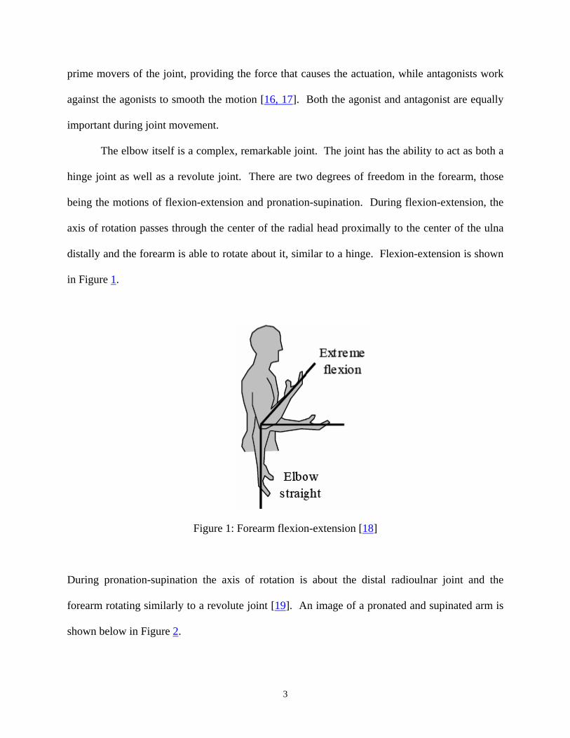
The elbow itself is a complex, remarkable joint. The joint has the ability to act as both a
hinge joint as well as a revolute joint. There are two degrees of freedom in the forearm, those
being the motions of flexion-extension and pronation-supination. During flexion-extension, the
axis of rotation passes through the center of the radial head proximally to the center of the ulna
distally and the forearm is able to rotate about it, similar to a hinge. Flexion-extension is shown
in Figure 1.
Figure 1: Forearm flexion-extension [18]
During pronation-supination the axis of rotation is about the distal radioulnar joint and the
forearm rotating similarly to a revolute joint [19]. An image of a pronated and supinated arm is
shown below in Figure 2.
3
Page 13
Figure 2: Forearm pronation-supination [ ] 18
Table 1 shows each muscle and their roles in flexion-extension and pronation-supination.
Several muscles are active during a given motion of the arm, making these forces somewhat
redundant.
Table 1: Primary elbow muscles and their roles in motions
Muscle Flexion Extension Pronation Supination
Biceps Brachii Agonist Antagonist Antagonist Agonist
Brachialis Agonist Antagonist Not active Not active
Brachioradialis Agonist Antagonist Antagonist Agonist
Pronator Teres Not active Not active Agonist Antagonist
Triceps Antagonist Agonist Not active Not active
4
Page 14
In a healthy elbow, the axis of rotation during flexion-extension is believed to be fixed and
constant, and the axis of rotation during pronation-supination has been measured to deviate by a
maximum of 1.5 millimeters [19, 20]. These metrics are examples of parameters that can be
used to evaluate prosthetic elbow implants and compare against current surgical practices.
1.2 BRIEF OVERVIEW OF JOINT SIMULATORS In an effort to effectively test the various surgical techniques and prosthesis designs used to treat
a radial head fracture, a device capable of simulating physiological motion of the elbow under
“real” loading conditions is needed. Currently, there are two methods of joint control. They are
manually and automatically-controlled, with the automatic-control consisting of either open or
closed-loop.
Only one report of an automatically controlled elbow simulator exists in the open
literature. It is an elbow simulator at the University of Western Ontario, in London, Canada, that
employs open-loop control of the muscle forces to actuate an arm [20]. This simulator allows
the tendons to be controlled through independent loads, applied directly to the tendons of the
forearm [21]. Despite the physiologic considerations, it has its shortcomings, including the lack
of antagonistic muscle control and achieving the desired arm motions that can require several
iterations [21]. This method of force control has also been shown to lack the ability to achieve
accurate positioning [21]. Regardless, this represents the most advanced elbow simulator
reported. An improved simulator for wrist joints exists at the University of Syracuse; a closed-
loop simulator that implements proportional-integral-derivative (PID) control to provide force
5
Page 15
control through the antagonist muscles and position control through the agonists [22]. The
marriage of force and position control in this system seems to be the most effective method for a
control system of the upper extremity.
1.3 CONTRIBUTIONS OF THIS WORK This work is concerned with developing an advanced motion simulator for the elbow joint. The
need for improving the method of restoration of proper elbow function following radial head
fracture is clear, and in order to do so, a test-bed for both prosthesis design and surgical
techniques is required. The proposed system combines various methodologies utilized in
previous studies and actuators [21, 22] and creates a method for manipulating the elbow in a
“real” manner through flexion-extension and pronation-supination by controlling the five major
muscles across the elbow joint. There is also an opportunity for expansion of this simulator’s
capabilities by investigating algorithm development for the implementation of neuromuscular
control.
6
Page 16
2.0 JOINT SIMULATORS There are several existing systems that are capable of simulating motion in various joints. These
various simulators and their methods of operation will be reviewed, along with their limitations.
2.1 OVERVIEW To date, joint simulation has been achieved in joints such as the knee, elbow, wrist, and shoulder.
Existing simulators employ several methods of joint control. One method is basically passive
control of the specimen, and it consists of the operators manually placing the joint at various
orientations, while measuring the variables of interest [4, 23, 24]. Another type manually
actuates the specimen through applied external forces [25, 26]. In these studies, the objective
was to duplicate loads at various joint positions rather than move the joint throughout a large
range of motion. Knee simulators exist that apply known forces to bones to study the effects on
the joint [25, 26]. Other simulators apply forces to the tendons rather than the bones to maintain
a position and examined the joint under those conditions [27, 28]. A final method uses external
force control to automatically actuate the limb by applying forces directly to the tendons,
allowing for study of continuous motion of the joint [21, 22, 29]. Each technique has its
shortcomings. In the manual method, the loading of the joint is not based on physiologic data,
and therefore can be subject to question. Furthermore, measurements can only be acquired at
discrete times, restricting the data. Externally controlled operation, although more meaningful,
7
Page 17
also has its limitations. Force control without position control hinders a simulator’s ability to
reach a desired position. One report combines force and position control in a wrist joint
simulator and currently, there are no elbow simulators that operate under these guidelines [22].
The vast majority of simulators are based on open loop control and include shoulder
simulators that apply constant loads to the muscles of the shoulder and utilize motion controlled
devices that attach to the bone to measure joint motion [30, 31]. There are also elbow simulators
that employ similar methods [32, 33].
There are also existing joint simulators that control the forces applied to the specimen
through a known time-history [34, 35]. A knee simulator at Vanderbilt University uses motion-
controlled motors to simulate knee flexion, using a load-controlled motor to apply the
compressive force. Loads are applied directly to the bone using a desired force time history [34].
Similarly, another knee simulator uses knee flexion time histories at McGill University in
Montreal to model walking. Stepper motors are connected directly to the tendons, and
displacement is controlled [35]. While a viable method for knee simulators, the use of time
histories is not yet possible in the upper limb since an accurate time history has not yet been
determined. There is, at least, a report of an elbow simulator discussed in the next section whose
concepts of design and operation can be leveraged in this effort.
2.2 UNIVERSITY OF WESTERN ONTARIO ELBOW SIMULATOR The most advanced device used for elbow testing found in the open literature was designed and
developed at the University of Western Ontario [21]. Cadaver elbows are controlled in the
vertical, varus, or valgus orientations. The simulator utilizes pneumatic actuators to
8
Page 18
simultaneously apply quasistatic loads to five tendons to create motion. The muscles of interest
represented by these actuators were the biceps, brachialis, brachioradialis, triceps, and the
pronator teres.
The simulator is designed in an effort to reproduce physiologic motion. A cadaver arm is
securely clamped to the apparatus so as to stabilize the specimen. Cables that attach to each
tendon are strategically positioned in order to reproduce each muscle’s physiological line of
action. The biceps, brachialis, and triceps were modeled by passing their cables through a set of
pulleys and to their respective tendons. The cables corresponding to the brachioradialis and
pronator teres are routed through pulleys and then through delrin sleeves implanted in the
humerus before attaching to the tendons.
In order to calculate the ratio of each muscle’s load, a combination of each muscle’s
cross-sectional area (CSA) and electromyographic (EMG) data was used. Relative loading in
each actuator was then determined based on these ratios. The achieved motion pathways of the
elbow reported are as repeatable as those obtained using a load-controlled simulator.
The motion of the radius and ulna relative to the humerus is monitored using an
electromagnetic tracking device. However, since the system is open-loop, the response is not
predictable, and several iterations are often required to produce the desired motions. Varying
specimen characteristics affect the response in each case, requiring different load levels to
produce the same motion. Questions arise concerning the validity of predicting forces based on
EMG and CSA data, since the study’s investigators questioned this technique due to the lack of
verification of the EMG – force relationship [21]. Also, the activation of the muscles from this
simulator differs from other published data [36, 37, 38].
9
Page 19
Many aspects of the Ontario elbow simulator translate to the proposed elbow simulator.
For example, similarities arise in the selection of muscles, clamping the specimen, and multi-
functional capabilities of the frame [21]. While its methods of control are not used, improved
control strategies will be incorporated from a wrist simulator outlined in the next section.
2.3 SYRACUSE UNIVERSITY WRIST SIMULATOR The only closed-loop, upper-extremity joint simulator found in the open literature is a dynamic
wrist simulator at Syracuse University [22]. The purpose of the machine was to be able to move
a cadaver wrist through various planar and non-planar motions. Hydraulic actuators manipulate
the wrist to achieve targeted movements. Six major tendons of the wrist are controlled to
simulate planar flexion-extension motions, planar radial-ulnar deviation motions, and combined
motions. Loads are applied as high as 267 N (60 lbs) to each tendon and produce motions of at
least ±30º. The cable positions are adjustable so that they are as close as possible to the
anatomical locations of the tendons. Antagonist muscles that resist the desired motion are
included in the simulator, serving to prevent slack in the muscles that are not being contracted,
allowing the limb to respond smoothly and quickly to muscle contractions.
The control algorithm operates via a hybrid position and force feedback using
Proportional-Integral-Derivative (PID) control. Agonists, or the prime movers, are controlled
through position feedback while antagonist muscles are excited with a constant force. Although
the antagonist force is expected to vary during motion, no information on how it varies is
available. A force transducer is connected in series with the hydraulic cylinders and the tendon
clamps to provide the force feedback signal. The transducer is constructed from a four-leg strain
10
Page 20
gage Wheatstone bridge fastened to a thin piece of aluminum, and it provides the force feedback
signal to the control algorithm. A three-degree of freedom electrogoniometer measures flexion-
extension and radial-ulnar deviation. The electrogoniometer records the motion and an A/D
board processes the forces from the transducer, and the cylinder forces are then adjusted
accordingly, thus closing the loop and allowing for control [22].
The dynamic wrist simulator has been successful in actively moving cadaver forearms to
determine the forces in the wrist tendons during ‘physiologic motion.’ Its innovative method of
design and control provides a valuable precedent for future simulators, including the one
described in this work.
2.4 PROPOSED SIMULATOR While each of the previously mentioned simulators are well-designed and have been shown to
accomplish their intended tasks, components of each can be extracted to construct the more
advanced simulator that is proposed in this thesis. Design features from the simulator at the
University of Western Ontario, such as the method of securing the specimen, the custom-
designed pulley system, the frame’s ability to rotate for varus/valgus testing, and muscles used to
manipulate the arm will be incorporated [21]. Also, the control algorithms used in the wrist
simulator at Syracuse University that operate using a combination of force and position feedback
will be implemented in the proposed simulator to achieve optimal control [22]. The simulator
will allow the arm specimen to achieve full range of motion in both flexion-extension and
pronation-supination, as well as allow for testing the specimen in varus/valgus orientations.
11
Page 21
3.0 SURVEY OF PHYSIOLOGIC KINEMATIC DATA A critical requirement of any joint motion simulator is that the system is arranged in a manner as
close to physiological as possible. The specimen must be able to move unhindered in the desired
planes of motion within the range of interest. Several experiments have been published that
measure variables of interest within the arm such as moment arms and change in various angles
with respect to joint motion.
3.1 MOMENT ARMS Moment arms about the rotating joint of each muscle must be reproduced in a mechanical device
attempting to reconstruct physiological joint motion [15, 39, 40, 41, 42]. In order to calculate the
proper placement of the self-designed pulley systems, published experiments were surveyed for
applicable kinematic information.
Moment arm data from several sources is shown below in Figures 3, 4, 5, 6, and 7 with
the muscles of interest being the biceps, the brachialis, the triceps, the brachioradialis, and the
pronator teres [15, 39, 40, 41, 42]. One study investigated the moment arms of ten specimens
and reported moment arm data for each [42]. Moment arms within this range were assumed to
be acceptable considering each plot of the moment arms versus flexion angle chiefly followed
the same trend for each individual muscle. As seen from the figures, there is a great deal of
discrepancy in the literature between the moment arm data for each muscle from study to study.
12
Page 22
Determination of the relevance of each study is important when analyzing the data. It is worth
noting that the data from Pigeon et al is a based on a computer model of the forearm, not an
actual arm specimen [43].
0
10
20
30
40
50
60
0 50 100 150Elbow Flexion (deg)
Mom
ent A
rm (m
m) Amis [39]
Gonzalez [40]Lemay [41]Pigeon [43]Murray M [15]Murray F [15]Murray [42]Murray [42]
Figure 3: Biceps moment arms
0
10
20
30
40
50
60
0 20 40 60 80 100 120 140 160
Elbow Flexion (deg)
Mom
ent A
rm (m
m)
Amis [39]Gonzalez [40]Lemay [41]Pigeon [43]Murray M [15]Murray F [15]Murray [42]Murray [42]
Figure 4: Brachialis moment arms
13
Page 23
-35
-30
-25
-20
-15
-10
-5
0
0 20 40 60 80 100 120 140 160
Elbow Flexion (deg)
Mom
ent A
rm (m
m)
Amis [39]Gonzalez [40]Lemay [41]Murray M [15]Murray F [15]Pigeon [43]Murray [42]Murray [42]
Figure 5: Triceps moment arms
0
10
20
30
40
50
60
70
80
90
100
0 20 40 60 80 100 120 140 160
Elbow Flexion (deg)
Mom
ent A
rm (m
m)
Amis [39]Gonzalez [40]Lemay [41]Murray M [15]Murray F [15]Pigeon [43]Murray [42]Murray [42]
Figure 6: Brachioradialis moment arms
14
Page 24
0
5
10
15
20
25
30
35
0 20 40 60 80 100 120 140 160
Elbow Flexion (deg)
Mom
ent A
rm (m
m)
Amis [39]Lemay [41]Murray M [15]Murray F [15]Murray [42]Murray [42]
Figure 7: Pronator teres moment arms
Discrepancies such as these are expected considering the variation of test subjects. Factors such
as age, sex, body type, and even whether the specimen is a right or a left hand can affect the
results of these experiments. As such, since there can be no guaranteed “correct” moment arm
for any muscle, it becomes more important to create a line of action with each cable that is
within the established range of acceptable results.
3.2 RELEVANT ANGLES Another significant factor in designing the pulley system is the angular change in each muscle’s
line of action as the arm moves. A cable running through a pulley needs to go as straight as
possible along the axis perpendicular to the pulley’s center axis of rotation to minimize losses in
the cable due to friction. Acceptable and unacceptable cable orientations within a pulley are
shown in Figure 8.
15
Page 25
Acceptable cable alignment
Unacceptable cable alignment
Figure 8: Pulley cable alignment
Coordinates of each of the five muscles’ origins and insertions are given in Table 2. The
coordinates for the origin and insertion points were taken from existing literature [44]. The
origins are the points of attachment that are fixed during contraction, and the insertions are points
of attachment to the bone that moves. The insertions are the points on the arm specimen where
each cable will attach. These attachment sites are known as tendonous insertions, because the
muscle itself does not attach to the bone, but rather to tendons, which are tough bands of fibrous
tissue that act as connectors between muscle and bone [44].
16
Page 26
Table 2: Elbow muscle origins and insertions [44]
Origin Insertion
Muscle X (cm) Y (cm) Z (cm) X (cm) Y (cm) Z (cm)
Brachialis 1.0 -0.6 20.0 0.0 1.2 -33.5
Biceps 2.5 0.0 1.0 -0.8 -0.2 -36.0
Triceps -0.8 -1.0 -16.0 -1.5 -2.0 -28.0
Brachioradialis 0.0 1.5 -27.0 0.0 0.0 -54.5
Pronator Teres -0.5 3.5 -29.0 0.5 -2.0 -43.5
The coordinates in Table 2 are centered about a body-fixed coordinate system with the origin
fixed at the center of the humeral head. They were measured in an erect standing position with
the arm hanging vertically and the forearm fully supinated. The axis of rotation for flexion-
extension is -30.5 cm along the z-axis in the humeral coordinate system. This humeral
coordinate system is shown in Figure 9.
17
Page 27
z z
y x
Figure 9: Humeral coordinate system [44]
The angles are determined by recalculating the insertions of each muscle as the arm rotates, then
implementing trigonometric relationships between the origin and calculated insertions
throughout the movement within the plane of interest. The method for determining the various
insertion coordinates of the muscles can be found in Appendix D in the MATLAB™ function
“angles.m.” Determining these angles will dictate the design of the pulley system. Small
angular variations will allow a pulley to be secured at a fixed orientation and still maintain an
18
Page 28
acceptable line of action within the pulley (see Figure 8). Large angular variations will require a
pulley that is capable of rotating with the specimen to prevent friction between the cable and the
sides of the pulley.
During flexion-extension, the “upper muscles,” that is, the biceps, brachialis, and triceps
main angle of interest is that within the lateral plane. These angles are shown below in Figures
10, 11, and 12.
Figure 10: Change in biceps angle through flexion-extension in coronal plane
19
Page 29
Figure 11: Change in brachialis angle through flexion-extension in coronal plane
Figure 12: Change in triceps angle through flexion-extension in coronal plane
20
Page 30
As shown in the figures, there is very little variation in this angle during flexion-extension for
each muscle. The biceps varies about 0.1º, the brachialis about 0.25º, and the triceps about 1.5º,
none of which are significant. Therefore, a pulley mounted with a fixed orientation will
experience little friction and is acceptable for the design.
Special care must be taken during pronation-supination of the forearm because the radius
rotates about the ulna. The center of rotation for this motion is taken to be about an oblique line
from the center of the radial head to where the radius and the ulna meet distally [44]. Figures 13
and 14 below show the change in the brachioradialis and pronator teres angles during pronation-
supination within the sagittal plane at 90º of flexion. At 0º of pronation, the forearm is in the
fully supinated position.
Figure 13: Change in brachioradialis angle through pronation-supination
21
Page 31
Figure 14: Change in pronator teres angle through pronation-supination
As seen in the Figures 13 and 14, through 100º of pronation-supination, the brachioradialis varies
about 9º and the pronator teres about 11º. The change in angle in these two muscles during
pronation-supination is substantial enough that they cannot be modeled using a pulley in a fixed
orientation, but rather requires a pulley system capable of rotating to accommodate this change.
The requirements for the pulley design have been presented in this chapter; the actual
design and the fulfillment of these requirements will be discussed later in Chapters 4 and 5.
22
Page 32
4.0 SIMULATOR DESIGN The completed elbow simulator is shown in Figure 15. The testing set-up is comparable to the
set-up employed in the previously described elbow simulator design [21]. A humeral clamp
secures the cadaver specimen to the frame. Five electromechanical actuators are mounted to the
frame, one actuator corresponding to each of the five major muscles that cross the elbow
(brachialis, biceps, triceps, brachioradialis, and pronator teres). The actuators control cables that
pass through realignment pulleys and attach to the tendons and/or tendonous insertions of the
forearm. Pulleys that connect the cable directly to the specimen are referred to as “primary”
pulleys, while all other pulleys in the system are called “secondary” pulleys. The custom-
designed pulleys are positioned so that they maintain each muscle’s line of action, as will be
further discussed in Chapter 5. The frame in Figure 15 is described in further detail below.
23
Page 33
“Upper Level” Center Align Secondary
Figure 15: Completed elbow simulator
4.1 FRAME DESIGN
The frame assembly for the elbow simulator was designed to be able to support all of the
necessary components of the simulator (actuators, pulley system, humeral clamp). Ample
structural integrity provides stability to prevent vibrations that would affect the movement of the
Electric Cylinders
Secondary PulleysPrimary
Pulleys Pulley
Frame Rotation
Humeral Clamp “Lower Level”
Guides Secondary
Pulleys
24
Page 34
cadaver specimen, while capable of rotating ±90º to simulate varus/valgus motion in addition to
flexion-extension. The humerus can be fixed horizontally or vertically, where in the latter the
forearm is able to move through its full range of flexion-extension. In the horizontal orientation,
the humerus is fixed parallel to the ground with the medial elbow inferior or superior to test
varus or valgus motion respectively [45]. The frame is over-designed in both its selection of
material and its structural strength to provide the desired functionality and stability.
In order to manipulate the cadaver specimen, pneumatic actuators control a cable that
pulls a different tendon. The actuators are manufactured by Exonic Systems (model no. ETB50
and ETB80) and have up to 200 mm (7.87 in) of stroke length [46]. They are mounted to the
frame on the end opposite the specimen and are positioned based on their respective muscle’s
approach to the elbow (see Figure 15). The brachialis, biceps, and triceps all run parallel to the
humerus and then into their respective insertions on the forearm, so they are positioned above the
specimen so the cables can then be re-directed down to the arm in a physiological manner.
Because these pulleys are mounted to the top level of the frame, they are referred to as “upper-
level pulleys”. Conversely, the brachioradialis and pronator teres originate near the humeral
head and then run parallel to the forearm to their insertion points, so these cylinders are mounted
with their vertical centers parallel to the forearm when it is positioned at 90º of flexion. These
pulleys will be referred to as “lower-level pulleys,” because they are mounted to the lower level
of the frame. A cable attached to the end of the actuators is aligned through a pulley alignment
system and then connected to the specimen. Ample space is provided between the actuators and
the secondary pulleys so that the actuators are free to move throughout their entire range of
motion without inadvertent contact between the two. The cables run through the re-alignment
pulley system to the specimen, which is held securely by a clamp on its humeral shaft.
25
Page 35
The humeral clamp is mounted to the front side of the frame and is aligned so that the
centerline of the humeral shaft centered horizontally on the frame, as seen in Figure 15. The
cadaver is supported by the clamp in four locations on the exposed section of the humerus. One
side of the clamp is fixed in place so that the specimens’ centerlines are kept constant from
experiment to experiment. The other side of the clamp can be adjusted in either direction to fit
the specimen, and the heads of the clamp are free to rotate about a setscrew so that they can stay
in the appropriate plane throughout adjustment. The entire clamp is also mounted to threaded
rods so that it can be adjusted vertically from specimen to specimen. A schematic of the
clamping system is shown in Figure 16.
Vertical Adjustment Nuts
Adjustable
Figure 16: Specimen clamping system
Since the frame also needs to have the capability to rotate ±90º, and because of its tendency to
slide rather than rotate if unrestrained, the bottom of the frame has small cylinders on both the
Stationary Clamp
Clamps
Horizontal Adjustment
Nuts
Specimen
26
Page 36
front and rear ends that are constrained to the ground by locking brackets. These cylinders act as
guides for rotating the frame. The brackets can be removed from one side, allowing the frame to
rotate about the cylinders on the other side for testing in varus or valgus orientations. This
rotation guide and locking system is illustrated in Figure 17.
Locking Bracket
Rotation Cylinder
Figure 17: Frame rotation guide
Several small locking brackets are placed along the base of the frame to hinder any vibration of
the system. These brackets can also be removed to allow the frame to rotate, then can be locked
again around the new base.
27
Page 37
4.2 CABLE SYSTEM DESIGN As previously mentioned, preserving the physiological line of action of the muscles is vital to
ensuring an accurate representation of the elbow’s motion, and this is accomplished via the
positioning of the pulleys that direct the cable to the desired insertions on the specimen.
4.2.1 “Upper-Level” Pulleys The “upper-level” pulleys are the pulleys that are located on top of the frame and the muscle’s
line of action runs along the humeral shaft and they are the brachialis and the biceps. From the
cylinders, the cables first pass through a set of “secondary” pulleys that are shown in Figure 18.
Tension From Spring
From Actuator To Center Alignment Secondary Pulley
Figure 18: “Upper-level” secondary pulley (top face removed)
Because the cables must run as straight as possible from the cylinders to the first pulley, the set is
placed directly in front of the respective cylinder. When a cable is attached to the cylinder and
28
Page 38
loaded through the pulley system, it would be impossible to prevent the presence of slack in the
line, so a tensioning pulley is positioned so that it can be adjusted and then secured to
compensate for up to two inches of slack in the cable.
The cable passes through this pulley to the “center-alignment secondary” pulleys, which
can be seen below in Figure 19.
To Primary Pulley
Figure 19: “Center-alignment secondary” pulleys
This set of pulleys consists of two pulleys that are at the same height as the previous set of
secondary pulleys, with one side higher than the other to compensate for the different heights of
each of the top cylinders. The entire block can be rotated 180º in the event that the biceps and
brachialis cylinders are swapped to switch from a right to a left arm specimen. The cable wraps
around the pulley and is redirected to the primary pulleys at the front of the frame.
29
Page 39
The primary pulleys redirect the cable over the front of the frame and to the specimen and
are shown below in Figure 20.
From Secondary Pulleys
To Specimen
Figure 20: “Upper-level” primary pulley
For the two actuators on top of the frame, the biceps and brachialis, this final pulley sticks out
over the edge of the frame, allowing the cable to run in front of the humeral shaft to each
insertion point. This final pulley’s placement for the brachialis will always remain constant, so it
30
Page 40
is fixed in its position in the center, but the biceps will switch sides, depending on whether the
specimen is a right or a left arm. Therefore, there is a primary pulley for the biceps on both sides
of the center pulley, and only one will be used at a time.
Although the triceps acts along the length of the humeral shaft and inserts into the
forearm like the biceps and brachialis, its pulley is positioned more distally than the “upper-
level” pulleys since it inserts behind the elbow.
4.2.2 Triceps Pulleys The cylinder representing the triceps is secured on underside of the cross-member that also
supports the biceps and brachialis in the horizontal center. Because it is centered, it only needs
one set of secondary pulleys to provide tension. The secondary pulleys are shown in Figure 21.
31
Page 41
From Cylinder
To Primary Pulley
Tension From Spring
Figure 21: Secondary triceps pulley (front face removed)
The primary pulley design for the triceps is similar to that of the biceps and brachialis, except
that it is mounted underneath the front cross-member. The primary triceps pulley is shown in
Figure 22.
32
Page 42
From Secondary Pulleys
To Specimen
Figure 22: Primary triceps pulley
4.2.3 “Lower-Level” Pulleys As previously mentioned, the muscles on the lower level of the frame, the brachioradialis and
pronator teres are mainly responsible for pronation-supination. These muscles originate on
either side of the humeral head and insert on the forearm. The actuators for the brachioradialis
and pronator teres are positioned so that their centers are aligned with the secondary pulleys,
which are very similar to the triceps’ secondary pulleys, but the third pulley is positioned lower
than the first pulley so it is in line with the first pulley in the primary set. The secondary pulley
system for the “lower-level” muscles in shown below in Figure 23.
33
Page 43
Tension From Spring
From Cylinder
To Primary Pulleys
Figure 23: “Lower-level” secondary pulleys (front face removed)
The line of action for these muscles is difficult to model with pulleys for several reasons. First
of all, both muscles’ origins are on the humeral head, so in order to accurately represent the
muscle, the cable would have to be as close as possible to the bone, which is not easily
accomplished. Secondly, as the arm is flexed, the line of action changes in two dimensions, so
the pulley must be designed to accommodate changes in both directions simultaneously. The
lower-level pulleys shown below in Figure 24 are capable of doing so.
34
Page 44
To Specimen
From Secondary Pulley
Figure 24: “Lower-level” primary pulleys
The arm that it is attached to the vertical pulleys can rotate about the horizontal pulley as shown
in the figure to provide a straight line of travel throughout pronation-supination. Additionally,
using this horizontal pulley as the center of rotation is important because this allows the cable to
travel a straight line between pulleys regardless of how much the system has rotated. After
passing the first horizontal pulley, the cable then wraps around under one vertically positioned
pulley and over another, whereby upon exiting this pulley, the cable has the freedom to track any
angle of flexion-extension. Also, wrapping the cable around this pulley is what provides the
radial force on the inner edge of the pulley’s groove that rotates the pulley arm.
The springs that were chosen to provide tension in the cable were initially selected
arbitrarily. As the testing becomes more dynamic, it will become increasingly evident how stiff
the spring must be to maintain the cable’s tension and allow the system to operate unhindered.
35
Page 45
4.2.4 Pulley Selection The pulleys that are used in the custom-designed pulley guides must be capable of withstanding
the loading conditions during experimentation, must be low-friction to minimize losses in the
cable, and must be small enough to fit in their designed housings. The CPS-2038 zinc-plated
steel pulleys from Sava Industries, Inc. were determined to be a suitable fit. They are precision-
machined ball bearing pulleys specifically grooved for small cables. The pulley’s outer diameter
is 0.500”, can handle cable sizes up to 3/64”, and can withstand a radial load capacity of up to
160 N at 50 RPM [47]. While higher load pulleys may be required in the future as the loads
increase, these pulleys will suffice to satisfy the current requirements.
4.2.5 Cable Selection
The cable connection between the electric cylinders and the muscle insertion points is made with
a high strength fishing line, inspired by the cable selection of the University of Western Ontario
elbow simulator [21]. The line that is used must be strong enough to withstand the loads it will
be subjected to during testing of an arm specimen, but must also have a smaller outer diameter
than the 3/64” the pulleys can accommodate. The Stren® Super Braid 80 lb. test is made of
braided Spectra® fiber was chosen for the tests. The 80 lb. test (~356 N) provides ample
strength in the initial stages of testing. While a stronger line may be required in the future as the
tests become more elaborate, this line meets all preliminary strength requirements. The Super
Braid’s outer diameter is rated at 0.020”; less than the maximum diameter of 0.046875” the
pulleys require [48].
36
Page 46
4.3 CONTROL SYSTEM In order to control an arm specimen when it is mounted in the completed frame, an advanced
control system is required. A five-axis controller is coupled with five electrically driven
cylinders from Exonic Systems that attach to the tendons and has the ability to achieve flexion-
extension and pronation-supination movements with a given specimen. Only five of the eight
axes on the controller are used currently, the remaining three are available for future
modifications. The ultimate goal is to automatically control the arm specimen using feedback
from position and force data, allowing flexion-extension, pronation-supination, or both
simultaneously in a physiological and meaningful manner. The complete control system setup is
shown below in Figure 25.
37
Page 47
ACR8020 Controller Card
To PCI Bus
DB37 Cable
Acroloop RBD Breakout Box
Axis FeedbackConnections
Secondary Breakout Box
50 Pin I/O Connector
Gemini Servo Drive
Motor
Electric Cylinders
Figure 25: Control system setup
A critical first step in controlling the system is the selection and implementation of the hardware
required.
38
Page 48
4.3.1 Hardware
4.3.1.1 Compumotor Hardware The “brain” of the control system is the controller card.
The ACR8020 controller card from Compumotor is its premier controller for PCI bus operation.
The card is a Digital Signal Processor (DSP) based, 32-bit floating point controller, with a multi-
tasking operating system that allows up to 24 tasks to be run simultaneously. It has up to eight
axes for servo or stepper motors (although only five are required by this application) and comes
equipped with 64 digital optically isolated input channels. Coupled with the ACR8020 card is
Compumotor’s RBD Breakout Module. This is a general application breakout board and it
features screw terminals for encoder position feedback for each of the eight axes as well as screw
terminals for the 64 digital inputs. All commands to and from the ACR8020 first pass through
the RBD Breakout Module before they are executed.
Individual control of each axis is provided by Gemini servo drives/controllers from
Compumotor. Each drive is easily configurable using its RS-232 port and its corresponding
software, Compumotor’s Motion Planner™, enabling it to receive commands from the ACR8020
card. The drive is capable of operating under several modes of operation, including torque,
velocity, step and direction, or clockwise/counter-clockwise, depending on the system’s
requirements. However, since the Acroloop card only provides position feedback, it is the
control mode that is used. Commands are sent from the drives to the motors, and feedback is
returned to the drives, allowing for optimal position control of each axis [49].
4.3.1.2 Secondary Breakout Box Although Compumotor produces all of the aforementioned
equipment, due to the flexibility the products provide in terms of compatibility with various
motors, drivers, and controllers, connectors are not provided to make the all of the necessary
39
Page 49
connections between each component. Rather, as in the case of the servo drive’s 50 pin I/O
connection, a single-ended connector cable is provided, leaving the other end open to wire
accordingly, depending on the desired method of control (torque, velocity, step/direction, etc.).
Therefore, a secondary breakout box was constructed to provide a casing for the interconnects
that must be made between the Acroloop card, the encoder feedback channels on the Acroloop
RBD breakout box, and between the I/O connection port on the servo drives. This secondary
breakout box can be seen above in Figure 25, and Figure 26 below shows a typical axis
connection, in this case, Axis 1. Detailed connections and their specific functions for this
breakout box are outlined in Appendix A.
40
Page 50
RBD Breakout Box Axis 1
A+
A-
B+
B-
Z+
Z-
+5V
GND
Green
Black
White
Blue
Red
Black
Black
Black
Orange
White/Orange
Blue
White/Blue
Yellow
White/Yellow
Red
Black
White/Brown
Brown
10 Row Terminal Block
50 Pin I/OConnector Cable
Gemini Servo Drive
DB 37 Connector
To AcroloopCard
Secondary BreakoutBox
Figure 26: Axis 1 connections in secondary breakout box
With the various instruments set up to operate together, a control programming language is
required that is not only powerful enough to process the incoming data and transmit the
necessary commands to the rest of the system, but also basic enough to allow for simplified
programming and debugging.
4.3.2 Software
The Acroloop motion control system is programmed using Compumotor’s program language,
Acroview, which simplifies programming, debugging, and executing an application [49]. The
“Setup Wizard” feature guides the user through the setup and configuration of the controller and
other hardware. The program and ladder editors allow basic motion command execution, as well
as developing I/O application code.
41
Page 51
The versatility and capabilities of the control system creates a framework for expansion
of the simulator. However, the design of the simulator must satisfy the criteria discussed in
Chapter 3. Ultimately, the hardware and software will be used to create a combination force and
position feedback control system that would close the loop and automatically control a specimen.
42
Page 52
5.0 FULFILLING KINEMATIC REQUIREMENTS
Chapter 3 presents the requirements for moment arms and angles when simulating muscles and
accurately recreating their lines of action; this chapter discusses how those requirements are met.
5.1 SIMULATOR MOMENT ARMS In a real arm, the muscle attachment sites to the fixed portion of the specimen are referred to as
origins. The aim in designing the pulley system in this simulator was not to reproduce the exact
muscle origins as found in the literature. Therefore, the leading edge of the each pulley will
represent that muscle’s “virtual origin.” These virtual origins are then converted to the same
coordinate system used for the points in Table 2. While they are quite different that the actual
muscle origins in the published literature, they serve a functional purpose in recreating the line of
action within each muscle. The insertions are taken from Table 2, and the virtual muscular
origins in the humeral coordinate system are shown below in Table 3. The number in
parentheses represents the adjustable range of each origin. Three orthographic views with
dimensions for each of the pulleys, representing the virtual origins, are provided in Appendix B
as Figures 37, 38, and 39.
43
Page 53
Table 3: Virtual muscle origins in the elbow simulator
Muscle X (cm) Y (cm) Z (cm)
Biceps 5.9 (-2.5) ±0.8 31.4
Brachialis 5.5 (-2.5) 0.0 33.3
Triceps -3.0 0.0 25.1
Pronator Teres 2.7 5.0 (±2.5) 2.5
Brachioradialis 2.7 -5.0 (±2.5) 2.5
A flowchart illustrating the moment arm calculations is shown in Figure 40 in Appendix C. The
MATLAB™ program “moments.m” in Appendix E calculates the moment arms for each muscle
during flexion-extension from 0° to 140°, using the functions “rot.m” in Appendix D and
“perp.m” in Appendix E. The results for each muscle are shown below in Figures 27, 28, 29, 30,
and 31 along with the highest and lowest moment arms from the literature for each muscle, and
the averages of each data set. The average standard deviation is also shown on each plot.
-10
0
10
20
30
40
50
60
0 20 40 60 80 100 120 140 160
Elbow Flexion (deg)
Mom
ent A
rm (m
m)
Our ResultsBiceps HighBiceps LowMean
Figure 27: Biceps moment arm results
44
Page 54
0
10
20
30
40
50
60
0 20 40 60 80 100 120 140 160
Elbow Flexion (deg)
Mom
ent A
rm (m
m)
Our ResultsBrachialis HighBrachialis LowMean
Figure 28: Brachialis moment arm results
-35
-30
-25
-20
-15
-10
-5
0
0 20 40 60 80 100 120 140 160Elbow Flexion (deg)
Mom
ent A
rm (m
m)
Our ResultsTriceps HighTriceps LowMean
Figure 29: Triceps moment arm results
45
Page 55
0
10
20
30
40
50
60
70
80
90
100
0 20 40 60 80 100 120 140 160
Elbow Flexion (deg)
Mom
ent A
rm (m
m)
Our ResultsBrachioradialis HigBrachioradialis LowMean
Figure 30: Brachioradialis moment arm results
-5
0
5
10
15
20
25
30
35
0 20 40 60 80 100 120 140 160
Elbow Flexion (deg)
Mom
ent A
rm (m
m)
Our ResultsPronator HighPronator LowMean
Figure 31: Pronator teres moment arm results
46
Page 56
The pulleys for the biceps, brachialis, pronator teres, and brachioradialis are adjustable, so their
respective moment arms will change as the pulleys are moved throughout their range of
adjustment. Each muscle’s range of moment arms are shown below in Figures 32, 33, 34, and
35.
Figure 32: Range of biceps’ moment arms
47
Page 57
Figure 33: Range of brachialis’ moment arms
Figure 34: Range of pronator teres’ moment arms
48
Page 58
Figure 35: Range of brachioradialis’ moment arms
The moment arms are chiefly in concurrence with the published moment arm data for these five
muscles [15, 39, 40, 41, 42]. As seen in the figures, each muscle’s moment arm follows the
same trend as the published data and falls within the range of established results. Slight
discrepancy is noted for the biceps above 130°, but the error is at the end of the flexion-extension
range and is acceptable. Although the insertion points will vary from specimen to specimen due
to several criteria, which is to be expected, the virtual origins are positioned such that the
moment arms that are reproduced will be suitable for testing.
The moment arms for the biceps and pronator teres during pronation-supination are also
of interest, but due to the lack of any published data, there is no precedent by which to verify
them. When this data appears in literature, calculations will be made to ensure these moment
arms are also acceptable.
49
Page 59
The cable system has been shown to meet its physiological requirements as prescribed
through testing in the open literature; its functionality must be verified using a test specimen
before it can be tested on an arm cadaver.
5.2 OPERATION VERIFICATION Due to variability, uncertainty, and the frequency of unforeseen occurrences during preliminary
experimentation, verification of the system is first performed on a wooden arm model that is
representative of an actual arm specimen. The model is shown below in Figure 36.
50
Page 60
Figure 36: Mock wooden arm for testing
It is essential that the arm model maintain the important characteristics of an actual arm for
testing purposes. Among these characteristics are functionality (flexion-extension, pronation-
supination), size (length, diameter) of the bones, location of the elbow joint with respect to the
humerus, ulna, and radius, the path of the active muscles, and the moment arms of those muscles.
To achieve the arm’s two degrees of movement, the wooden model uses a construction
similar to anatomical human skeletal models for teaching purposes. A simple pin joint inserted
through the ulna and the humerus proximally allows for the flexion-extension motion, and it is
capable of achieving the full range of motion native to real arms. For the pronation-supination
motion, a pin joint inserts into the radial head along the shaft of the radius. A small bracket
51
Page 61
attached to the distal end of the radius rotates about a pin at the distal end of the ulna, allowing
for pronation-supination while securing the two together. Eyehooks were inserted as close to the
published insertions as possible. The cables were attached to the cylinders, wound through the
pulley systems, and then tied to the eyehooks on the arm.
Open loop control was used to manipulate the arm. Muscles were displaced through
known distances to achieve flexion-extension, pronation-supination, and both motions at the
same time. While this method of control is crude and relatively simple, it is successful in
moving the wooden arm and verifying the operation of the simulator. Based on the literature and
the results of the cable system design, the integrity of each muscle’s line of action is preserved
and proves to be fully functional for testing.
Although not implemented into testing, Appendix F illustrates a program that moves two
actuators at different amplitudes and directions of a sine wave of the same period.
52
Page 62
6.0 CONCLUSIONS AND FUTURE WORK
6.1 SUMMARY A device has been designed and fabricated that is capable of manipulating a cadaver arm
specimen in a meaningful and physiological manner throughout its full range of motion. This
elbow motion simulator utilizes electromechanical actuators to simulate muscle action within the
arm. Custom-designed pulley guides align the cable system to establish a correct positioning for
the origins of each muscle and maintain them throughout the travel of the arm. The insertion
points were determined by surveying the body of literature for the forearm muscle groups. A
humeral clamp secures the specimen via the humeral shaft to maintain an accurate position.
Rudimentary open-loop testing using a mock forearm constructed from wood demonstrated that
the test frame performs as expected. Following this work, a closed-loop control algorithm needs
to be developed with a combination of position and force feedback. The algorithm will be
implemented and tested on a wooden arm model first, and then on a real arm specimen. The
creation of this simulator and the further development of the control algorithms will allow
investigation into a range of studies involving the arm.
53
Page 63
6.2 ELBOW FUNCTION In-vitro studies of the elbow joint will be performed to augment knowledge of the elbow. There
are many questions regarding the kinematics of the normal and pathological elbow. Limitations
in the study of elbow motion have been experienced by previous researchers, but can be
overcome by this elbow simulator. The effects of varying radial head orientation and placement
will be studied in a radial head replacement and compared to forearm kinematics in a normal
arm, an area that has not been addressed in the literature.
6.3 DYNAMIC STUDIES
The simulator can be used to study ligament reconstruction and dynamic elbow movement.
While static tests have been previously conducted, no work has moved the arm physiologically.
This simulator will simultaneously flex/extend and pronate-supinate the arm at speeds as fast as
300°/sec. This speed will be able to reproduce a flexion-extension motion in about the same
amount of time as that of an average adult. Concurrent movements will be studied at physiologic
speeds. Additionally, the simulator will move the forearm with a 7-kg weight attached to the
hand, flexing completely in about 5 seconds. Elbow replacement design must consider complex
movements and large load capacity. This simulator will test the replacements under
physiological loading conditions, moved at physiological speeds.
54
Page 64
6.4 NEURAL CONTROL STUDIES Several theories exist on the neural process used for motor control, such as sum of the squares of
neural activations or the weighted sum of a function of muscle forces [50, 51]. These theories
are based solely on computer models of the forearm. This simulator can validate neuromuscular
control theories rather than focus solely on model validation. Robotic arms attached to
humanoid robots have been stabilized using simple neural circuits [52]. These devices can now
be examined under the dynamics and non-linearities of the human system.
55
Page 65
APPENDIX A: HARDWARE CONNECTION DETAILS
Table 4: DB37 to Acroloop card connections
5
4
3
2
1
Axis Connector Pin No. DB 37 Cable Wire ColorFunction
24 Black/Blue -10V CMD
5 White/Red +10V CMD
23 White/Blue -10V CMD
4 Red +10V CMD
22 Blue -10V CMD
3 Black/Brown +10V CMD
21 Black/Teal -10V CMD
2 White/Brown +10V CMD
20 White/Teal -10V CMD
1 Brown +10V CMD
56
Page 66
APPENDIX B: DIMENSIONS OF PULLEY POSITIONS
All dimensions are in centimeters
66.0
33.0
32.2 32.2
33.0
66.0
28±2.5 28±2.5
Figure 37: Frame front view
57
Page 67
33.3
31.4
25.1
2.5
Figure 38: Frame right view
58
Page 68
4.3±1.3 2.7 4.7±1.3
Figure 39: Frame top view
59
Page 69
APPENDIX C: FLOWCHART FOR MOMENT ARM CALCULATION
Calculate new coordinates of insertions after flexing through
specified angle
Angle of flexion-
extension
Input muscle origins
Output moment arms
Calculate perpendicular distance between the line from the origin to the insertions and
the center of the axis of rotation
Input muscle insertions
Figure 40: Moment arm calculation flowchart
60
Page 70
APPENDIX D: MATLAB™ CODE FOR ANGULAR DATA %angles.m %Calculate change in angles for forearm muscles during motion %Muscle origins and insertions [44] %Biceps origins bi_o = [2.5, 0, 1.0]; bi_i = [-0.8, -0.2, -36.0]; %Brachialis origins br_o = [1.0, -0.6, 20]; br_i = [0, 1.2, -33.5]; %Triceps origins tr_o = [-0.8, -1, -16]; tr_i = [-1.5, -2, -28]; %Brachioradialis origins bd_o = [0, -1.5, -27]; bd_i = [0, -3, -54.5]; %Pronator teres origins pt_o = [-.5, 3.5, -29]; pt_i = [.5, -2, -43.5]; %Vector with angles from 0 to 140 deg. in multiples of 5 angle = linspace(0, 140, 29); %calculate angles for flexion-extension for i = 1:29 %run 'rot.m' function bi_i_new = rot(bi_i, angle(i)); br_i_new = rot(br_i, angle(i)); tr_i_new = rot(tr_i, angle(i)); %Calculate angle from muscle origin and array of insertions bi_angle(i,:) = atan((bi_o(2) - bi_i_new(2))/(bi_o(3) – bi_i_new(3))); br_angle(i,:) = atan((br_o(2) - br_i_new(2))/(br_o(3) – br_i_new(3))); tr_angle(i,:) = atan((tr_o(2) - tr_i_new(2))/(tr_o(3) – tr_i_new(3))); end %calculate angles for pronation-supination angle_ps = linspace(0, -100, 21); %Move insertions to 90 deg flexed position bd_i = rot(bd_i, 90); pt_i = rot(pt_i, 90); for i = 1:21 %run 'rot_ps.m' function bd_i_new = rot_ps(bd_i, angle_ps(i)); pt_i_new = rot_ps(pt_i, angle_ps(i)); %calculate angle from muscle angle and array of insertions bd_angle(i,:) = atan((bd_o(2) - bd_i_new(2))/(bd_o(1) – bd_i_new(1))); pt_angle(i,:) = atan((pt_o(2) - pt_i_new(2))/(pt_o(1) - pt_i_new(1)));
61
Page 71
end %convert radians to degrees bi_angle = bi_angle * 180/pi; br_angle = br_angle * 180/pi; tr_angle = tr_angle * 180/pi; bd_angle = bd_angle * 180/pi; pt_angle = pt_angle * 180/pi; %plot results figure; plot(angle, bi_angle); xlabel('Flexion Angle (deg)'); ylabel('Angular Variation (deg)'); figure; plot(angle, br_angle); xlabel('Flexion Angle (deg)'); ylabel('Angular Variation (deg)'); figure; plot(angle, tr_angle); xlabel('Flexion Angle (deg)'); ylabel('Angular Variation (deg)'); figure; plot(-angle_ps, bd_angle); xlabel('Pronation Angle (deg)'); ylabel('Angular Variation (deg)'); figure; plot(-angle_ps, pt_angle); xlabel('Pronation Angle (deg)'); ylabel('Angular Variation (deg)');
62
Page 72
%function rot.m %Determine new muscle insertion after flexion %Input variables %% 'ins': insertion points %% 'angle': angle of rotation %Output variables %% 'ins_new': new insertion coordinates after rotation function [ins_new] = rot(ins, angle); %Convert degrees to radians angle = angle*pi/180; %Make coordinate system about elbow (axis of rotation) ins(3) = ins(3) + 30.5; %Rotation matrix [53] R = [cos(angle) 0 -sin(angle); 0 1 0; sin(angle) 0 cos(angle)]; %Calculate new insertions and move z-coord back to humeral CS ins_new = R * [ins]'; ins_new(3) = ins_new(3) - 30.5;
63
Page 73
%rot_ps.m %calculates angle throughout 100 deg of pronation-supination %Input variables %% 'ins': insertion points %% 'angle': angle of rotation %Output variables %% 'ins_new': new insertion coordinates after rotation function [ins_new] = rot(ins, angle); %Convert degrees to radians angle = angle*pi/180; %Make coordinate system about elbow (axis of rotation) ins(3) = ins(3) + 30.5; %Rotation matrix R = [1 0 0; 0 cos(angle) -sin(angle); 0 sin(angle) cos(angle)]; %Calculate new insertions and move z-coord back to humeral CS ins_new = R * [ins]'; ins_new(3) = ins_new(3) - 30.5;
64
Page 74
APPENDIX E: MATLAB™ CODE FOR MOMENT ARM DATA %moments.m %Calculate moment arms through 140 deg of flexion %Prompt for muscle origin orig_x = input('Muscle Origin x: '); orig_y = input('Muscle Origin y: '); orig_z = input('Muscle Origin z: '); orig = [orig_x, orig_y, orig_z]; %Prompt for muscle insertion ins_x = input('Muscle Insertion x: '); ins_y = input('Muscle Insertion y: '); ins_z = input('Muscle Insertion z: '); ins = [ins_x, ins_y, ins_z]; %Vector with angles from 0 to 140 deg. in multiples of 5 angle = linspace(0, 140, 29); %Calculate moment arms throughout motion for i = 1:29 %run 'rot.m' function ins_new = rot(ins, angle(i)); %run 'perp.m' function moment(i) = perp(orig, ins_new); end
65
Page 75
APPENDIX F: SINUSOIDAL MOVEMENTS IN TWO CYLINDERS REM THIS PROGRAM TAKES A SINE WAVE AND MOVES TWO CYLINDERS... REM IN OPPOSITE DIRECTIONS AND AT DIFFERENT FREQUENCIES PROG0 HALT ALL REM HALTS ALL MOTION COMMANDS NEW ALL REM CREATES A NEW PROGRAM DETACH ALL REM DETACHES ALL AXES ATTACH MASTER0 REM DEFINES MASTER0 ATTACH SLAVE0 AXIS0 "X" REM ATTACHES SLAVE AXIS0 "X" ATTACH SLAVE1 AXIS1 "Y" 10 ACC10 DEC10 VEL10 STP10 REM CREATES MOTION PROFILE 20 X3 Y3 REM MOVES X AND Y AXIS TO 3 INCHES REM MOVE X IN SINUSOID ENDING AT 0 DEG WITH 0 DEG PHASE... REM 1440 DEG AND AMPLITUDE OF 3 REM MOVE Y IN SINUSOID ENDING AT 0 DEG WITH 180 DEG PHASE... REM 1440 DEG AND AMPLITUDE OF 1 30 SINE X(0,0,1440,3) SINE Y(0, 180, 1440, 1) 40 END
66
Page 76
%function perp.m %Calculate perpindicular distance from muscle to center of %rotation %Input variables %% 'orig': muscle's origin coordinates %% 'ins': muscle's insertion coordinates %Output variables %% 'dist': calculated moment arm function [dist] = per(orig, ins); x1 = orig(1); y1 = orig(2); z1 = orig(3); x2 = ins(1); y2 = ins(2); z2 = ins(3); A = [x2-x1,y2-y1,z2-z1,0;1,0,0,x1-x2;0,1,0,y1-y2;0,0,1,z1-z2]; B = [0;x1;y1;z1]; point = A\B; dist = sqrt((point(1)^2)+(point(2)^2)+point(3)^2);
67
Page 77
BIBLIOGRAPHY [1] Gordon M, Bullough PG. Synovial and osseous inflammation in failed silicone-rubber
prostheses: a report of six cases. J Bone and Joint Surgery 1982; 64(4):574-580.
[2] Morrey, BF, 1993. Radial head fractures. In: Morrey, BF (Ed.), The Elbow and its Disorders, second ed. WB Saunders Company, Philadelphia, pp. 383-404.
[3] Hotchkiss RN, Weiland AJ, Valgus stability of the elbow. J Orthop. Res. 1987; 5(3): 372-377
[4] Morrey, BF, Tanaka S, An KN. Valgus stability of the elbow. Clin Orthop. 1991 Apr; (265): 187-95.
[5] Ring D, Jupiter JB, Zilberfarb J. Posterior dislocation of the elbow with fractures. J Bone and Joint Surgery; 2002 Apr; 84-A(4):547-551.
[6] Morrey BF, An KN. Articular and ligementous contributions to the stability of the elbow. Amer Journal of Sports Med; 1983 Sep-Oct; 11(5):315-319.
[7] London JT. Kinematics of the elbow. JBJS; 1981 Apr; 63(4); 529-535.
[8] Stroyan M, Wilk KE. The function anatomy of the elbow complex. J Orthop Sports Phys Ther; 1993 Jun; 17(6): 279-288.
[9] Trousdale RT, Amadio PC, Cooney WP, Morrey BF. Radio-ulnar dissocation. A review of twenty cases. JBJS; 1992 Dec; 74(10): 1486-1497.
[10] Beingessner DM, Dunning CE, Beingessner CJ, Johnson JA, King GJ. The effect of radial head size on radiocapitellar joint stability. Clin Biomech; 2003 Aug; 18(7): 677-681.
[11] Hotchkiss, RN. Displaced fractures of the radial head. J Amer Acad Ortho Surgeons; 1997; 5: 1-10.
[12] Moro JK, Werier J, MacDermid JC, Patterson SD, King GJ. Arthroplasty with a metal radial head for unreconstructible fractures of the radial head. JBJS; 2001 Aug; 83-A(8): 1201-1211.
68
Page 78
[13] Olsen BS, Vaesal MT, Sojbjerg JO, Helmig P, Sneppen O. Lateral collateral ligament of the elbow joint: anatomy and kinematics. J Elbow and Shoulder Surg; 1996 Mar-Apr; 5(2 Pt 1): 103-112.
[14] Chao EY, Morrey BF. Three-dimensional rotation of the elbow. J Biomech; 1978; 11(2): 57-73.
[15] Murray WM, Delp SL, Buchanan TS. Variation of muscle moment arms with elbow and forearm position. J Biomech; May 1995; 28(5): 513-525.
[16] Colbaugh R, Glass K. Hierarchical control of human joint motion simulators. Comp & Elec Eng; 1993 May; 19(3): 213-230.
[17] Winters JM, Stark L. Analysis of fundamental human movement patterns through the use of in-depth antagonistic muscle models. IEEE Trans Biomed Eng; 1985 Oct; 32(10): 826-839.
[18] Armstrong T, Ebersole M. Occupational Ergonomics Posture Analysis Exercise. 23 July 2003. http://www-personal.engin.umich.edu/~tja/TaskForcePosture.pdf (25 July 2004).
[19] Hollister AM, Gellman H, Waters RL. The relationship of the interosseous membrane to the axis of rotation of the forearm. Clin Orthop; 1994 Jan; (298): 272-276.
[20] Sauerbier M, Fujita M, Hahn ME, Neale PG, Berger RA. The dynamics radioulnar convergence of the Darrach procedure and the ulnar head hemiresection interposition arthroplasty: a biomechanical study. J Hand Surg; 2002 Aug; 27(4): 307-316.
[21] Johnson JA, Rath DA, Dunning CE, Roth SE, King GJW. Simulation of elbow and forearm motion in vitro using a load controlled testing apparatus. J Biomech; May 2000; 33(5): 635-639.
[22] Werner FW, et al. Wrist joint motion simulator. J Orthop Res; 1996 Jul; 14(4): 639-646.
[23] King GJW, Itoi E, Niebur GL, Morrey BF, An KN. Motion and laxity of the capitellocondylar total elbow prosthesis. JBJS; 1994;76-A: 1000-1008.
[24] Olsen BS, Sojbjerg JO, Nielsen KK, Vaesel MT, Dalstra M, Sneppen O. Posteolateral elbow joint instability: the basic kinematics. J Shoulder Elbow Surg; 1998 Jan-Feb; 7(1): 19-29.
[25] Ahmed AM, Burke DL, Zsombor-Murray PJ. Design aspects of an apparatus for the static loading of two-component synovial joints. Biomech Symposium; 1997; American Society of Mechanical Engineers, New York: 223-226.
[26] Lorry BS, et al. An in-vitro test system for conducting multi-axial load-displacement tests on diarthrodial joints. ASME; 1991;120;141-144.
69
Page 79
[27] Hollis JM. A six-degree-of-freedom test system for the study of joint mechanics and ligament forces. J Biomech;1995 Nov;117(4): 383-389.
[28] Kihara H, Short WH, Werner FW, Fortino MD, Palmer AK. The stabilizing mechanism of the distal radioulnar joint during pronation and supination. J Hand Surg; 1995 Nov; 20(6): 930-936.
[29] King GJW, Zarzour ZD, Rath DA, Dunning CE, Patterson SD, Johnson JA. Metallic radial head arthroplasty improves valgus stability of the elbow. Clin Orthop; 1999 Nov; (368): 114-125.
[30] Cain PR, Mutschler TA, Fu FH, Lee SK. Anterior stability of the glenohumeral joint. A dynamic model. Am J Sports Med; 1987 Mar-Apr; 15(2); 144-148.
[31] Sharkey NA, Marder RA, Hanson PB. The entire rotator cuff contributes to elevation of the arm. J Orthop Res; 1994 Sep; 12(5): 699-708
[32] Bottlang M, O’Rourke MR, Steyers CM, Marsh JL, Brown TD. Radiographic determinants of the elbow rotation axis: experimental indentification and quantitative validation. J Orthop Res; 2000 Sep; 18(5): 821-828.
[33] Madey SM, Bottlang M, Steyers CM, Marsh JL, Brown TD. Hinged external fixation of the elbow: optimal axis alignment to minimize motion resistance. J Orthop Trauma; 2000 Jan; 14(1): 41-47.
[34] DiAngelo DJ, Harrington IA. Design of a dynamic multi-purpose joint simulator. Advances in Bioeng; 1992; ASME, BED-Vol 22: 107-110.
[35] McLean CA, Ahmed AM. Design and development of an unconstrained dynamic knee simulator. J Biomech; 1993 May; 115(2): 144-148.
[36] Buchanan TS, Rovai GP, Rymer WZ. Strategies for muscle activation during isometric torque generation at the human elbow. J Neurophysiol; 1989 Dec; 62(6): 1201-1212.
[37] Caldwell GE, Jamison JC, Lee S. Amplitude and frequency measures of surface electromyography during dual task elbow torque production. J Appl Physiol Occup Physiol; 1993; 66(4): 349-356.
[38] Tax AA, Denier van der Gon JJ, Gielen CC, Kleyne M. Differences in control of m. biceps brachii in movement tasks and force tasks. Exp Brain Res; 1990; 79(1): 138-142.
[39] Amis AA, Dowson D, Wright D. Muscle strengths and musculo-skeletal geometry of the upper limb. Eng in Med; 1979 Jan; 8(1): 41-48.
[40] Gonzalez RV, Hutchins EL, Barr RE, Abraham LD. Development and evaluation of a musculoskeletal model of the elbow joint complex. J Biomech; 1996 Feb; 118(1): 32-40.
70
Page 80
[41] Lemay MA, Crago PE. A dynamic model for simulating movements of the elbow, forearm, and wrist. J Biomech; 1996 Oct; 29(10): 1319-1330.
[42] Murray WM, Buchanan TS, Delp SL. Scaling of peak moment arms of elbow muscles with upper extremity bone dimensions. J Biomech; 2002 Jan; 35(1): 19-26.
[43] Pigeon P, L’Hocine-Yahia, Feldman AG. Moment arms and lengths of human upper limb muscles as functions of joint angles. J Biomech; 1996 Oct; 29(10): 1365-1370.
[44] Seireg A, Arvikar R. Biomechanical Analysis of the Musculoskeletal Structure for Medicine and Sports. Hemisphere Publishing Corporation, New York, NY, 1989.
[45] Dunning CE, Duck TR, King GJW, Johnson JA. Simulated active control produces repeatable motion pathways of the elbow in an in vitro testing system. J Biomech; 2001 Aug; 34(8): 1039-1048.
[46] Parker Automation. ET Series Stepper and Servo Driven Linear Actuators, 1 Jan 1998.
[47] Steel pulleys. Carl Stahl Sava Industries, Inc. 1998-2004. http://www.savacable.com/catalog/p27-steelpulleys.htm (1 Apr 2004).
[48] Stren Super Braid. Stren. 2004. http://www.stren.com/line_braid.htm (1 Jul 2004).
[49] Parker Automation. Gemini GV Hardware User’s Manual, 1 Dec 2001.
[50] Rehbinder H, Martin C. A control theoretic model of the forearm. J Biomech; 2001 June; 34(6): 741-748.
[51] Raikova R. A model of the flexion-extension motion in the elbow joint: some problems concerning muscle forces modeling and computation. J Biomech; 1996 June; 29(6): 763-772.
[52] Williams MM. Neural Control of Rhythmic Arm Movements. 1998, http://www.ai.mit.edu/projects/humanoid-robotics-group/cog/cog.html (1 April 2004).
[53] Spiegel M, Liu J. Schaum’s Outline of Mathematical Handbook of Formulas & Tables. McGraw-Hill, New York, NY, October 1998.
71